Emission line selected galaxies at in GOODS South: Stellar masses, SFRs, and large scale structure
Abstract
We have obtained deep NIR narrow and broad (J and Y) band imaging data of the GOODS-South field. The narrow band filter is centered at 1060 nm corresponding to redshifts for the strong emission lines H, Oiii/H and Oii, respectively. From those data we extract a well defined sample ( in the narrow band) of objects with large emission line equivalent widths in the narrow band. Via SED fits to published broad band data we identify which of the three lines we have detected and assign redshifts accordingly. This results in a well defined, strong emission line selected sample of galaxies down to lower masses than can easily be obtained with only continuum flux limited selection techniques. We compare the (SED fitting-derived) main sequence of star-formation (MS) of our sample to previous works and find that it has a steeper slope than that of samples of more massive galaxies. We conclude that the MS steepens at lower (below ) galaxy masses. We also show that the SFR at any redshift is higher in our sample. We attribute this to the targeted selection of galaxies with large emission line equivalent widths, and conclude that our sample presumably forms the upper boundary of the MS.
We briefly investigate and outline how samples with accurate redshifts down to those low stellar masses open a new window to study the formation of large scale structure in the early universe. In particular we report on the detection of a young galaxy cluster at which features a central massive galaxy which is the candidate of an early stage cD galaxy, and we identify a likely filament mapped out by OIII and emitting galaxies at .
Key Words.
Galaxies:high-redshift1 Introduction
The study of galaxies at both intermediate and high redshifts has gained tremendous momentum from the concerted efforts to gather deep imaging of large fields, and from the ensuing high quality photometry covering large spectral ranges. Analyses exploiting those data to derive prime observables such as star-formation rates (SFRs) and stellar masses have revealed that galaxies follow scaling relations that evolve with redshifts (Brinchmann et al. 2004; Noeske et al. 2007; Daddi et al. 2007). The most comprehensive investigations are based on multi-band photometry, and the ability to obtain redshift information via fitting of theoretical model data is a critical component (Daddi et al. 2007; Karim et al. 2011; Bayliss et al. 2011; Koyama et al. 2013). The photometric redshift accuracy also places a fundamental limitation on the results from the unavoidable uncertainty in the assignment of redshifts to each galaxy, an uncertainty which propagates to all the derived physical parameters of the galaxies.
There are different methods of addressing the galaxy formation and evolution quest. Galaxy samples are selected differently and therefore probe different aspects of galaxy evolution. Intensively starforming galaxies have been studied for nearly two decades thanks to the Lyman-break selection technique (Steidel et al. 2003; Shapley 2011). Flux limited high-redshift samples selected at primarily red wavelengths include Luminous Infrared Galaxies (LIRGs), Ultra Luminous Infrared Galaxies (ULIRGs), and massive () red ellipticals (Jacobs et al. 2011). Sub-mm selected samples target high-redshift galaxies with unprecedented star-formation rates (Michałowski et al. 2010; Hodge et al. 2013). Long-duration gamma-ray bursts (GRBs) select fainter and bluer star-forming galaxies (Le Floc’h et al. 2003; Christensen et al. 2004). Also here selection effects play a role, as GRB hosts have been suggested to have low stellar masses (Castro Cerón et al. 2010, e.g.,), while dusty GRBs occur preferentially in more massive host galaxies (Krühler et al. 2011). Absorption-line selected samples allow us to study the gas content of galaxies and can be used to probe the mass-metallicity relation (Ledoux et al. 2006; Møller et al. 2013; Christensen et al. 2014). In a nutshell, these methods all address different populations of galaxies and have different advantages and disadvantages for particular science goals.
In order to investigate the vs SFR relation for galaxies found in isolation and in clusters, none of these methods will simultaneously probe the low-mass end of the star-forming main sequence and cover intermediate-to-high redshifts. An alternative method that can help us in achieving this goal is the narrow-band imaging technique (Pritchet & Hartwick 1987, e.g.,). Emission-line selected samples are smaller, but the advantage is that they allow us to probe fainter objects than broad-band selected samples do and still have a much more accurate photometric redshift determination (Ly et al. 2012; Sobral et al. 2014). Narrow-band selected objects have excess flux in the narrow-band filter compared to a broad-band filter that covers adjacent wavelengths. Primarily, this technique has been used to detect high redshift Lyman- (Ly) emission lines because is a good tracer of galaxies at the beginning of the reionization era (Partridge & Peebles 1967; Malhotra & Rhoads 2004; Nilsson et al. 2007).
The scope of this paper is to fill in the knowledge gap concerning the low-mass end of the main-sequence of star-forming galaxies in a broad redshift range. We analyse emission-line sources selected from deep 1060 nm narrow-band ( hereafter) and - and -band observations of the GOODS-South field from Clément et al. (2012). The GOODS-South field is ideal for our objective as the field has been observed in a wide range of wavelengths and with a good photometric accuracy (Giavalisco et al. 2004) allowing for very detailed photometric scrutiny of sources in the field. When searching for emission-line galaxies at redshifts , we also detect galaxies with emission lines other than falling within the narrow-band filter. In this way, we can probe the universe in four independent redshift slices: besides the high-redshift line, we detect galaxies at from strong emission lines, at from Oiii/ emission lines, and where galaxies with strong Oii emission lines lie. We perform multi-band photometry SED fitting and derive masses and SFRs of 40 emission-line galaxies at three different redshift slices. We analyse the redshift evolution of the -SFR relation spanning more than four decades in stellar mass from a unique data set.
The paper is organized as follows: in Sect. 2 we describe candidate selection process and datasets used for this project. Sect. 3 characterizes spectroscopic and photometric properties of the selected galaxies and compare with redshifts from the MUSYC survey. Sect. 4 and 5 present the results and a discussion of these.
Throughout this paper, we assume a flat cosmology with , and a Hubble constant of km s-1 Mpc-1.
2 Selection of emission-line galaxies


2.1 Imaging observations
The GOODS South field was observed with VLT/HAWK-I in the 1060 nm narrow-band and broad J- and Y-band filters (see filter transmission curves in Fig.1) as part of a Large ESO Programme (Prog-Id: 181.A-0485, PI: Cuby) and a HAWK-I science verification programme (Prog-Id: 60.A-9284(B), PI: Fontana). For details on the observations and data reduction we refer to Castellano et al. (2010) and Clément et al. (2012). The field is in the northern half of the GOODS-S field (centred at RA,Dec = -, J2000).
2.2 Candidate selection
For object detection and photometry, we use the software package SExtractor (Bertin & Arnouts 1996). For the actual selection of candidate emission line galaxies we rely only on the Hawk-I , and -band images. As a detection image we use the narrow-band image, and photometry is subsequently done in all three images with aperture sizes defined in the image. Before object detection the detection image is convolved with a Gaussian filter function having a FWHM equal to that of point sources. We use a detection threshold of 1.5 times the background sky-noise in the unfiltered detection image and a minimum area of 15 connected pixels above the detection threshold in the filtered image. Isophotal apertures are defined on the detection image and those same isophotal apertures are used in the different bands (, , ). We reject objects close to the chip gap and the edge of the image where the noise is higher. The regions of the field masked out in this way are shaded grey in Fig. 15. In total, we detect 2700 objects at a signal-to-noise ratio greater than 5 in the narrow-band. We measure the flux of all objects in the isophotal aperture which is suitable for precise colour measurement as the effective seeing of the images are very similar. To get a measure of the total magnitudes we use the so-called AUTO aperture in SExtractor. The AUTO aperture is an elliptical aperture defined by the isophotal shape of the object. For objects blended with neighbours a scaled isophotal flux is used to estimate the total flux. Our final catalog is complete (10 detection) down to in the narrow-band.
In order to select objects with excess flux in the narrow-band we employ the method introduced by Møller & Warren (1993) and refined by Fynbo et al. (2003). This method uses two broad band filters which bracket the narrow-band. Plotting the two narrow-minus-broad colours against each other causes objects with an emission line within the narrow pass-band to drop diagonally down to the left (Fig. 2 upper panel). We compute the distribution of the cloud of continuum emitters using theoretical spectral energy distributions from Bruzual & Charlot (2003), and enclose the region where the model galaxies fall with a red dashed line in Fig. 2 (for details see Fynbo et al. (2003)). All objects in our catalog are plotted in Fig. 2, upper panel, and it is seen that most objects do indeed fall inside the red dashed line. The dotted blue line marks the selection window we have adopted below and to the left side of the main locus of continuum objects. For we select objects with . For we use . The 40 objects found inside this area, and at least 1 from the border, make up our ”basic sample”, they are listed in Table 1 and are highlighted red in Fig. 2. The basic sample is complete in the sense that we have included all objects within the unmasked area of the observed field down to , and it is therefore suitable for statistical studies within the unmasked area which spans 38.7 square arcminutes on the sky.
We searched the NED/IPAC11 1 The NASA/IPAC Extragalactic Database (NED) is operated by the Jet Propulsion Laboratory, California Institute of Technology, under contract with the National Aeronautics and Space Administration. and SIMBAD (Wenger et al. 2007) databases, and found spectroscopic, secure redshifts for a subset of the basic sample, as listed in Table 1.
As a check of the selection, the images were inspected in ds9 in RGB mode, with blue=Y, green=NB1060, red=J. Objects that looked green (i.e. showed some degree of narrow-band excess) and which looked like galaxies and not artifacts or noise were marked. The mask used in defining the basic sample was not used, i.e. also objects located in higher noise regions of the image were included. After removing the basic sample of 40 galaxies and the ELG00 galaxy, this visually-identified narrow-band excess sample comprised 58 objects. There were 3 not necessarily mutually exclusive reasons why these galaxies were not part of the basic sample: (1) their colours were outside the selection region, i.e. the observed EW was too low, (2) they were in a masked part of the image, or (3) they were fainter than NB1060(AUTO) = 24.8. SIMBAD was searched, and 18 of the 58 objects had a spectroscopic, secure redshift. For all 18 galaxies (named x01 to x18), the redshift matched an emission line, see Table 2. These 18 galaxies, as well as ELG00 (see below), do not fulfill our selection criteria and thus cannot be used in our basic sample, but together with the basic sample they form an “extended sample”.
In addition we obtained spectra and determined redshifts of two objects as described in Sect. 3.1. The two objects are highlighted by blue circles in Fig. 2, where one is seen to be in our basic sample (ELG55) while the other is directly to the left of the large cloud of galaxies. This is an intriguingly strange position since it shows that it has an emission line in the ( colour, but no line in the ( colour. It is not in the basic sample so we have named it ELG00 and it is listed in the first line of Table 2.
In Fig.19 we show , and HST W-band thumbnails (the latter is the deepest optical band we have) for all 40 galaxies in the basic sample, and also including ELG00 of the extended sample. As seen, all are indeed detected in the W-band and hence are not consistent with being Ly emitters at . The candidates have very mixed morphologies ranging from bright spirals over irregular galaxies with multiple cores, to very faint compact systems.
3 Characterization of the candidate emission-line galaxies
3.1 Spectroscopic observations
On March 15 and 16 2013 we secured redshift measurements for two objects in our catalog. The spectra were obtained with the X-shooter spectrograph (Vernet et al. 2011) installed at the Cassegrain focus of the Very Large Telescope (VLT), Unit 2 – Kueyen, operated by the European Southern Observatory (ESO) on Cerro Paranal in Chile (prog. ID 090.A-0147). The spectra were reduced with the ESO X-shooter pipeline 2.0 (Goldoni 2011). In Fig. 3 we show the X-shooter spectra around the region of the filter.
One of the object (ELG55, lower panel of Fig. 3) is belonging to the basic sample, and we see that the line is confirmed to Oiii5007 based on the detection of Oiii4959 and Oii3727 and the derived redshift is 1.1107.
| ID | RA DEC | Redshift | [Peak] | [min/max] | line ID | Em. Line flux | Eq.Width | Ref | |||
|---|---|---|---|---|---|---|---|---|---|---|---|
| (2000.0) | mag (AUTO) | mag (ISO) | mag (ISO) | This work | MUSYC | MUSYC | |||||
| 03 | 03:32:40.32 -27:47:22.71 | 0.61 | 0.60/0.63 | H | (1) | ||||||
| 04 | 03:32:44.30 -27:46:59.99 | 1.12 | 1.10/1.14 | Oiii | (2) | ||||||
| 05 | 03:32:36.30 -27:47:32.63 | 2.29 | 2.05/2.48 | Oii | (3) | ||||||
| 06 | 03:32:37.20 -27:47:25.56 | 1.85 | – | – | Oii | ||||||
| 09 | 03:32:41.34 -27:46:46.23 | 0.60 | 0.56/0.64 | H | |||||||
| 10 | 03:32:37.97 -27:46:51.86 | 0.63 | 0.62/0.63 | H | (4) | ||||||
| 11 | 03:32:42.76 -27:46:33.19 | 0.64 | 0.62/0.66 | H | |||||||
| 12 | 03:32:37.36 -27:46:45.52 | 2.26 | 2.22/2.31 | Oii | (5) | ||||||
| 14 | 03:32:36.83 -27:46:51.52 | 1.80 | 1.72/1.89 | Oii | |||||||
| 15 | 03:32:37.08 -27:46:47.03 | 1.93 | 1.84/2.04 | Oii | |||||||
| 16 | 03:32:35.81 -27:46:43.62 | 2.13 | 1.88/2.32 | Oii | (6) | ||||||
| 20 | 03:32:36.69 -27:46:20.98 | 1.90 | 1.80/2.00 | Oii | (3) | ||||||
| 21 | 03:32:37.45 -27:46:15.34 | 1.94 | 1.83/2.04 | Oii | |||||||
| 22 | 03:32:36.55 -27:46:12.28 | 1.94 | 1.90/1.98 | Oii | (3) | ||||||
| 23 | 03:32:39.52 -27:45:59.75 | 1.86 | 1.43/2.31 | Oii | |||||||
| 25 | 03:32:39.33 -27:45:55.14 | 1.90 | 1.75/2.04 | Oii | |||||||
| 26 | 03:32:45.73 -27:45:24.97 | 1.09 | 1.05/1.12 | Oiii | |||||||
| 28 | 03:32:27.82 -27:46:35.07 | – | – | Oiii | |||||||
| 30 | 03:32:30.03 -27:46:04.24 | – | – | Oiii/Oii/H | |||||||
| 34 | 03:32:26.60 -27:46:05.02 | 1.28 | 1.06/1.55 | Oiii | |||||||
| 35 | 03:32:21.53 -27:46:18.71 | 1.74 | 1.50/1.96 | Oii | |||||||
| 36 | 03:32:26.68 -27:45:54.79 | 1.18 | 1.09/1.30 | Oiii | |||||||
| 37 | 03:32:21.69 -27:46:16.57 | 2.45 | 2.32/2.59 | Oii | |||||||
| 41 | 03:32:21.26 -27:46:02.55 | 1.53 | 1.12/1.74 | Oii | |||||||
| 43 | 03:32:19.60 -27:46:08.31 | 1.07 | 1.05/1.09 | Oiii | |||||||
| 45 | 03:32:42.51 -27:44:15.55 | 0.61 | 0.60/0.63 | H | |||||||
| 51 | 03:32:16.50 -27:44:45.04 | 1.11 | 1.10/1.12 | Oiii/H | |||||||
| 52 | 03:32:41.59 -27:42:50.68 | – | – | Oiii | |||||||
| 53 | 03:32:13.15 -27:45:01.19 | 2.06 | 1.95/2.17 | Oii | |||||||
| 54 | 03:32:12.98 -27:44:59.81 | – | – | Oii | |||||||
| 55 | 03:32:16.31 -27:44:41.93 | 1.12 | 1.11/1.12 | Oiii | (*) | ||||||
| 58 | 03:32:41.68 -27:42:04.45 | 1.25 | 1.21/1.30 | Oiii/Oii | |||||||
| 62 | 03:32:34.22 -27:42:31.37 | 0.61 | 0.60/0.63 | H | |||||||
| 65 | 03:32:39.20 -27:41:44.69 | 1.14 | 1.12/1.15 | Oiii | |||||||
| 66 | 03:32:38.22 -27:41:45.51 | – | – | Oii/Oiii | |||||||
| 68 | 03:32:23.88 -27:42:11.56 | 1.60 | 1.50/1.70 | Oii | |||||||
| 70 | 03:32:33.03 -27:40:48.06 | 1.13 | 1.11/1.14 | Oiii | |||||||
| 75 | 03:32:30.36 -27:41:46.66 | – | – | Oii/Oiii | |||||||
| 76 | 03:32:22.75 -27:42:11.59 | 1.89 | 1.76/2.00 | Oii | |||||||
| 78 | 03:32:33.89 -27:42:37:92 | 0.64 | 0.64/0.65 | H | (7) |
(1) Ravikumar et al. (2007); (2) Xu et al. (2007); (3) Trump et al. (2011);
(4) Rodrigues et al. (2008); (5) Mignoli et al. (2005);
(6) Guo et al. (2012); (*) This work
(7) Balestra et al. (2010);
| ID | RA DEC | Redshift | line ID | Em.line flux | Eq.Width | Ref. | |||
|---|---|---|---|---|---|---|---|---|---|
| (2000.0) | spectroscpic | mag (AUTO) | mag (ISO) | mag (ISO) | |||||
| ELG00 | 03:32:18.57 -27:42:29.50 | H | (*) | ||||||
| x01 | 03:32:13.24 -27:42:40.03 | H | (1) | ||||||
| x02 | 03:32:23.40 -27:43:16.58 | H | (2) | ||||||
| x03 | 03:32:41.83 -27:40:42.31 | H | (1) | ||||||
| x04 | 03:32:38.59 -27:46:31.36 | H | (3) | ||||||
| x05 | 03:32:31.50 -27:41:58.04 | H | (1) | ||||||
| x06 | 03:32:45.65 -27:44:05.80 | H | (1) | ||||||
| x07 | 03:32:28.01 -27:43:57.44 | H | (4) | ||||||
| x08 | 03:32:40.79 -27:46:15.70 | H | (1) | ||||||
| x09 | 03:32:46.75 -27:46:24.02 | H | (5) | ||||||
| x10 | 03:32:22.25 -27:49:01.47 | Oiii | (6) | ||||||
| x11 | 03:32:27.66 -27:45:05.77 | Oiii | (6) | ||||||
| x12 | 03:32:26.77 -27:45:30.63 | Oiii | (6) | ||||||
| x13 | 03:32:18.81 -27:49:08.59 | Oiii | (7) | ||||||
| x14 | 03:32:49.83 -27:46:58.30 | H | (1) | ||||||
| x15 | 03:32:17.11 -27:42:20.95 | Neiii | (8) | ||||||
| x16 | 03:32:38.80 -27:47:14.82 | Oii | (9) | ||||||
| x17 | 03:32:18.43 -27:42:51.95 | Oii | (8) | ||||||
| x18 | 03:32:36.69 -27:46:48.48 | Oii | (10) |
(*) This work; (1) Balestra et al. (2010); (2) Vanzella et al. (2005); (3) Szokoly et al. (2004); (4) Le Fèvre et al. (2004); (5)Xia et al. (2011); (6) Vanzella et al. (2006); (7) Villforth et al. (2012); (8) Straughn et al. (2011); (9) Guo et al. (2012); (10) Trump et al. (2011);
The other object (ELG00, upper panel of Fig. 3) is not in the basic sample but was observed because of its strange position in the colour-colour plot as described in section 2.2 above. Here we see a strong H line (based on the detection of a wide range of other lines in the visual spectral region) and the derived redshift is 0.6045. The strong H line is located in the very wing of the filter curve as given by the ESO web page 22 2 http://www.eso.org/sci/facilities/paranal/instruments/hawki/inst/filters/hawki_NB1060.dat We do not detect the Nii6583 line in the spectrum.
3.2 Photometric redshifts


The very conservative selection criteria employed for our basic sample definition ensures that a strong emission line is present in the narrow-band filter. Therefore the task of redshift determination of our narrow band selected sample is reduced to determining which of the three most likely redshift groups each object belongs to, H, Oiii/H, or Oii. In a few cases we already have spectroscopic confirmations, for the remainder we rely on photometric redshift analysis. For this we take advantage of the variety of photometric data available for the GOODS field. We explored a wide range of available data sets, and in the end we concluded that the most robust results are obtained using primarily the available photometry from the CANDELS survey (Guo et al. 2013) (G13 hereafter). CANDELS is a survey including nearly 35000 sources combining data from among others HST-WFC3 and HST-ACS, VLT-VIMOS, VLT-HawkI, VLT-ISAAC and Spitzer/IRAC, spanning wavelengths from the UV to the near-infrared. The CANDELS catalogue contains magnitudes and magnitude errors for in total 17 different bands. To construct the catalogue a careful and complete source detection algorithm as well as flux derivation methods including aperture corrections were employed. However, no photometric or spectroscopic redshift information is provided in the catalogue.
For a subset of the objects Y-band (F105W) photometry was not available in G13 (the last 14 in Table 1). For these targets we added our own Y-band photometry (from HAWK-I) to the data sets before the SED fitting and redshift determination. For these objects we performed aperture photometry in circular apertures. The aperture size was matched to the apparent extension of the object on the sky. For each used aperture size we determine aperture corrections measured on isolated, unsaturated point-sources.
For the Spectral Energy Distribution (SED) fits we use the LePhare code (Arnouts et al. 1999; Ilbert et al. 2006). Those fits provide also a first photometric redshift probability distribution which we use to guide us towards the final “redshift slice” assignments for each object.
To construct the model SED we use the Bruzual and Charlot (BC03) spectral library (Bruzual & Charlot 2003). The library uses stellar evolutionary tracks for different metallicities and Helium abundances from the Padova 1994 stellar synthesis models. It generates spectra in the wavelength range from 3200 to 9500 at higher resolution and across wider wavelength range, 91 to with lower resolution, assuming Chabrier initial mass function (IMF) (Chabrier 2003) and the Calzetti extinction law (Calzetti et al. 2000). The ages for the model galaxies range from to yr. The code is based on the exponentially declining star formation history (SFH). We also include contribution from the emission lines in the models. For this, LePhare uses a simple recipe based on the Kennicutt (1998) SFR and UV luminosity relation. The code includes the strongest emission lines, like , , , Oiii doublet - and Oii, varying the ratio of the above-mentioned lines with Oii. For further details on LePhare code characteristics, see Ilbert et al. (2006) and the LePhare manual.


For each object we go through the following steps. We fit to the full set of photometric data twice, once using all data points, and once where we exclude the narrow band and the Y-band since they are both dominated by the emission line which may skew the fit. We then decide, after visual inspection of each individual fit, if there is a unique solution, or if two or even all three redshift solutions are possible. This is done independently by 4 of us and redshifts are only assigned if we all 4 agree. For most (35) objects there clearly is a unique solution, but for the remainder 5 objects no unique redshift assignment is possible this way. In 4 cases there is a best solution (dubbed “primary redshift” and listed first in Table 1) but also a possible secondary solution. In one case (ELG30) all three solutions are possible and none of them are preferred. ELG30 is the object which is in the lowest left corner of Fig. 2, i.e. it has larger emission line equivalent width than any other object in our sample. Presumably the strong emission lines are confusing the SED fit. All redshifts assigned in this way are provided in Table 1. As a final step we then repeat the SED fit but this time locking the redshift to the spectroscopic redshift (when available) or to the assigned redshift based on the identification of the emission line. The purpose of this last fit is to obtain the best fitted values for stellar mass and star formation rate.
In Fig. 4 we show examples of fits to three of the objects with unique solutions, one belonging to each redshift slice. We show both the first fit where the redshift was left as a free fitting parameter, and the final fit with assigned redshift.
3.2.1 The V-I vs Z-J redshift diagnostic plot

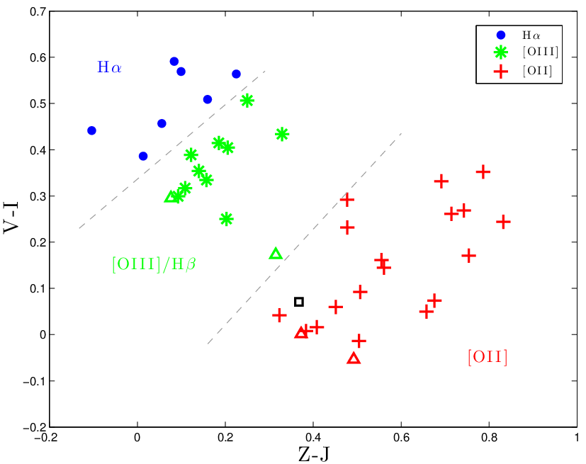
In Fig. 6 we plot the V-I colour versus the Z-J colour for all the unique object redshifts and the four primary but non-unique redshift solutions (open triangles). The objects are colour coded according to redshift slice (H blue, Oiii/H green, and Oii red). It is seen that the points separate out quite clearly in this diagram in agreement with the work by Bayliss et al. (2011). Galaxies move from the lower right towards the upper left in this diagram as they move to lower redshifts, and it is a coincidence that the internal scatter of the distribution at any given redshift forms a perfect match to the separation in redshift forced by the wavelengths of the three transitions. It is therefore possible to use this figure as a diagnostic plot to assist slice identification in cases where no unique solution can be found. Our primary redshifts are seen to agree well with this plot which is further support that those assignments are correct. We have also plotted the last object without redshift assignment (ELG30) as a black square, and we see that it is mostly embedded in the region occupied by Oii emitters, close also to Oiii emitters, but far away from H emitters.

We note that ELG30 has the highest equivalent width (EW) emission line of our sample, and that would suggest that it is an Oiii emitter since they in general have large EW (see e.g., Pénin et al. (2014)). Further insight into the redshift of ELG30 comes from Fig. 7, showing the observed-frame EW of the line in the NB1060 filter (as derived in Sect. 4.2) against the (F125WF160W) colour from the G13 catalogue. For (H in NB1060), no strong emission lines will be in neither F125W nor F160W. For ([OIII]5007 in NB1060), H will be in F125W while no strong lines will be in F160W. For (H in NB1060), no strong lines will be in F125W while H will be in F160W. For ([OII] in NB1060), H will be in F125W and [OIII]5007 will be in F160W. These considerations indicate that a high-EW line emitter with a blue (F125WF160W) colour such as ELG30 is more likely to be [OIII]5007 than [OII].
All things considered we are not able to assign a primary redshift to ELG30.
3.2.2 Cross-referencing with the MUSYC survey

In Fig. 8 we cross-check our final redshift assignments against those of the MUSYC survey (Cardamone et al. 2010). The MUSYC survey consists of imaging of the GOODS-South field in a wide range of broad and medium-wide filters. The MUSYC catalogue contains photometry for more than 84000 galaxies including the GOODS field. The catalogue lists magnitudes, photometric and spectroscopic (when available) redshifts and a large range of other characteristics. Photometric redshifts have been obtained using the EAZY (Easy and Accurate Zphot from Yale) photometric redshift code (Brammer et al. 2008). In Fig. 8 we plot the MUSYC redshifts against our redshifts, excluding six objects for which we could find no MUSYC counterpart. Two primary redshift assignments (ELG51 and 58) are marked with red triangles and the agreement is seen to be good. We therefore conclude that our redshift assignments for those two objects are secure. The last three non-secure redshifts have no counterparts in MUSYC.
It is seen from Fig. 8 that there is a very good agreement in the general trend, and the listed errors in the MUSYC catalogue give mostly a reasonably distribution of , notably for the lower redshift slices. However, four of the 18 certain OII emitters are off, one is at , and one at (the latter being ELG12, which has a spectroscopic redshift and which is detected in X-rays, and therefore possibly an AGN). We therefore conclude that while the general trend is in excellent agreement, and the errors for the slice are very small, for the two higher redshift slices the errors become increasingly larger, and for the slice the errors are in about 30% of the cases underestimated. Therefore galaxy scaling relations derived from large statistical samples based on only photo-z redshifts are probably reliable out to at least , but at higher redshifts there are significant, and in some cases significantly underestimated, errors on the redshifts which will propagate into errors on the derived physical parameters such as stellar masses () and star-formation-rates (SFR). At higher redshifts one might therefore obtain more accurate results from smaller samples but with more accurate redshifts.
3.3 Broad band flux depth
Our survey function is defined based on narrow band flux limit and emission line equivalent width. This means that we do not have any actual lower limit on broad band fluxes in our sample, and therefore our survey differs significantly from spectroscopic surveys where strict broad band flux limits are used for target selection to ensure a good probability that a redshift can be determined from the spectrum. We expect that our sample is deeper than spectroscopic surveys in the same field, and in order to assess how much we have extracted a complete spectroscopic sample from the catalog of Vanzella et al. (2008) (V08 hereafter). The V08 survey targeted galaxies in the GOODS-S down to a limiting magnitude of (AB) = 26, making it one of the deepest existing spectroscopic surveys (cf. Table 5 in Le Fèvre et al. (2015)).
From V08 we extracted all objects with redshift in one of our three redshift slices.In order to obtain a comparison sample of a good size we used slices of width 0.4, centered at the same redshifts, i.e. around = 0.62, 1.15 and 1.85. In Fig 9 we show the distribution of two broad band magnitudes (F435W(B) and F125W(J)) for both our basic sample (black histogram) and the V08 sample (grey histogram). In order to make the studies consistent, we obtained the photometry from the G13 catalog for all objects. It is seen that our sample is significantly deeper in both bands. The median of the comparison sample is 24.71 and 22.56 ( and respectively) while our sample has medians 25.49 and 24.92, i.e. our sample goes around 0.8 and 2.3 magnitudes deeper.
For example in the overlapping region between our survey and the recent catalog of HST grism spectroscopy (Morris et al. 2015) our sample has 33 objects at redshifts probed by the HST spectroscopy (), but the HST catalog contains only the seven brighter of those. The redshifts are all in agreement.

4 Results
4.1 The main sequence of star formation in three narrow redshift slices
The SED fits described in Sect. 3.2 also provide values for and SFR of each galaxy. We list those values in Table 3, and in Fig. 10 we plot SFR vs . Both in the local universe, and out to a redshift of 3.5, it has been shown that SFR forms a tight correlation with (Brinchmann et al. 2004; Noeske et al. 2007; Maiolino et al. 2008), the so called main sequence of star formation (MS). The MS has been shown to evolve with redshift and in Fig. 10 we have overplotted the relations from stacked radio data of star-forming galaxies reported in Table 4 of Karim et al. (2011) (full lines) at each of the redshifts of our three redshift slices. From Karim et al. (2011) we take the mean of their = 0.4–0.6 and 0.6–0.8 bins to represent , their = 1.0–1.2 bin to represent , and their = 1.6–2.0 bin to represent . Both the data and the relations are colour coded according to redshift slice as in Fig. 6. We also plot a vertical dashed line at log()=9.4 which is the lower limit of the samples considered by Karim et al. (2011). One object (ELG14) turned out to provide unstable physical parameters in the sense that leaving out a single photometric point would severely change the output parameters. Upon checking the HST image we noted a close neighbour galaxy of different colour which presumably could have affected the photometry and caused this. The redshift is good so we keep it in the sample, but we exclude it from the analysis of the MS relation. We also exclude ELG30 from this analysis since we do not have a redshift for it. We use the primary redshift solutions for ELG66 and 75, but repeat the analysis using the secondary solutions. No significant difference is found using the secondary solutions (see Table 4).
| ID | log(mass) | log(SFR) | Redshift | |
|---|---|---|---|---|
| ELG# | fixed | |||
| 3 | 9.01 | 0.06 | 0.619 | |
| 4 | 8.63 | 0.45 | 1.144 | |
| 5c | 9.12 | 1.41 | 1.86 | |
| 6 | 9.04 | 1.13 | 1.86 | |
| 9 | 8.15 | -0.90 | 0.62 | |
| 10 | 9.27 | 0.21 | 0.62 | |
| 11 | 7.86 | -0.91 | 0.62 | |
| 12c | 10.21 | 2.38 | 1.843 | |
| 14c | 8.67 | 0.76 | 1.85 | |
| 15c | 9.12 | 1.58 | 1.85 | |
| 16c | 9.87 | 1.52 | 1.85 | |
| 20c | 8.92 | 1.20 | 1.85 | |
| 21c | 8.89 | 1.07 | 1.85 | |
| 22c | 9.40 | 1.84 | 1.85 | |
| 23 | 8.74 | 0.74 | 1.85 | |
| 25c | 8.86 | 1.33 | 1.85 | |
| 26 | 8.85 | 0.36 | 1.15 | |
| 28 | 8.28 | -0.37 | 1.15 | |
| 34 | 8.48 | -0.63 | 1.15 | |
| 35 | 9.41 | 1.27 | 1.85 | |
| 36 | 8.31 | -0.38 | 1.15 | |
| 37 | 8.49 | 0.77 | 1.85 | |
| 41 | 8.89 | 1.02 | 1.85 | |
| 43 | 8.43 | -0.29 | 1.15 | |
| 45 | 8.50 | -0.55 | 0.62 | |
| 51 | 8.77 | 0.09 | 1.15 | |
| 52 | 8.43 | -0.62 | 1.15 | |
| 53 | 9.61 | 1.47 | 1.85 | |
| 54 | 9.06 | 1.53 | 1.85 | |
| 55 | 9.29 | 1.49 | 1.15 | |
| 58 | 8.68 | -0.11 | 1.15 | |
| 62 | 7.97 | -1.09 | 0.62 | |
| 65 | 8.61 | -0.06 | 1.15 | |
| 661 | 8.48 | 0.48 | 1.85 | |
| 68 | 9.10 | 0.61 | 1.85 | |
| 70 | 8.99 | 0.32 | 1.15 | |
| 751 | 8.50 | 0.88 | 1.85 | |
| 76 | 9.55 | 1.56 | 1.85 | |
| 78 | 9.77 | 1.10 | 0.624 | |
| Ambiguous cases | ||||
| 662 | 7.91 | 0.38 | 1.15 | |
| 752 | 8.02 | 0.49 | 1.15 | |
| 303 | 6.72 | -1.15 | 0.62 | |
| 303 | 7.31 | -0.82 | 1.15 | |
| 303 | 7.83 | -0.39 | 1.85 |
c - Cluster member galaxy.
1 - Primary fixed redshift solution used for ELG66 and 75.
2 - Secondary fixed redshift solution used for ELG66 and 75.
3 - No preferred redshift for ELG30, although H is disfavoured.

From Fig. 10 we see that our data roughly are in agreement with the relation from Karim et al. (2011), i.e. that there is a MS and that it evolves with redshift in the sense that galaxies of a given stellar mass have lower SFR at lower redshifts. Our data points are somewhat offset from the expected relations, but this could possibly be due to the fact that our objects sample a much lower stellar mass range than the relations we compare to. If the MS e.g. is steepening at the low mass end, it would cause our low mass galaxies to drop below the relations. In order to test this we first assume that the slopes reported by Karim et al. (2011) at each of our redshift slices are correct for all masses and then we determine the offsets to our data. The best fit offsets are shown as dashed coloured lines in Fig. 10 and provided in Table 4. We then remove the effect of redshift evolution in two different ways. First we assume that the evolution from Karim et al. (2011) is correct and we apply a shift which brings all galaxies (and the relations) to what they would have been in the Oii redshift slice (upper left panel of Fig. 11). We then fit a broken linear relation to the data points with the following two conditions: () at log() larger than 9.4 it must have the slope of 0.59 (from Karim et al. (2011)); and () it must be continuous in log()=9.4. The resulting best fit is shown in Fig. 11, lower left panel, and the best fit slope is found to be with an rms of 0.31. In the two right panels of Fig. 11 we show the same as in the left, only here we have applied redshift correction shifts such that the dashed lines in Fig. 10 are lined up rather than the full lines. In this case the best fit gives a slope of with an rms of 0.29.

| SFR offset | rms | ||
| 0.62 | 7 | 0.35 | |
| 1.15 | 121 | 0.43 | |
| 1.15 | 142 | 0.52 | |
| 1.85 | 191 | 0.27 | |
| 1.85 | 172 | 0.27 | |
| All | 381 | 0.32 | |
| All | 382 | 0.34 |
1 - Primary redshift solution used for ELG 66 and 75.
2 - Secondary redshift solution used for ELG 66 and 75.
Our sample reaches stellar masses 1.5 decades lower than the sample of Karim et al. (2011) and we see that in the range below their lower mass limit our sample follows a significantly steeper MS no matter how we correct for the redshift evolution. Previous analyses of the derived stellar masses from SED fits with exponential declining and increasing star-formation rates in a population of star-forming galaxies at z=1-2 have shown that the stellar masses vary within 0.1 dex (Christensen et al. 2012). As we noted above, the offsets we reported in Table 4 may in this case be dominated by this steepening of the slope, and we shall therefore repeat the fit using a more realistic assumption. Rather than assuming a constant slope we now use a slope with a break at log()=9.4. For the high mass end we use the slope of 0.59 from Karim et al. (2011), for the low mass end we use the mean of the slopes we found above, which is 1.17.


The resulting best fit is shown in Fig. 12 and again reported in Table 4. We see that allowing for the change of slope we now get a consistent positive offset towards higher SFR in all three redshift slices. This is no great surprise as one would expect samples selected by narrow band techniques to select the objects with the strongest emission lines in any stellar mass bin, and consequently to contain the highest SFR galaxies of any mass at any redshift. In that sense our sample defines the upper envelope of the MS for low to intermediate mass galaxies.
In conclusion of this section we first tested if our sample was offset (up or down) in SFR compared to Karim et al. (2011) and using their reported slope. We found an inconsistent scatter with both positive and negative offsets, but this could be because the median is different in the three redshift slices. We then removed the effect of redshift to make them more easy to compare, and noted evidence that the slope is steeper at low masses. Assuming a steeper slope in the low mass end we find that our data are consistent with a constant offset from the Karim et al. (2011) data (at 6.6) with an internal scatter of 0.32. Performing the same fit to the data, but instead using the constant slope of Karim et al. (2011) at all masses gives a zero offset with an internal scatter of 0.43 which is a significantly poorer fit even allowing for the one degree of freedom less.
4.1.1 Comparison with other studies
Whitaker et al. (2014) present MS fits from a study of galaxies in the CANDELS fields. At stellar masses larger than they use a UV+IR SFR indicator on photometry of individual photo-z galaxies, at lower stellar masses they do the same on stacked photometry and reach stellar masses of (at z=0.5) to (at z=2.5). Similar to our results of the previous section they report a steepening of the slope at lower masses but they fit it with a polynomial rather than a broken powerlaw. They also report a shallower redshift evolution of the MS at lower masses than at high masses. Lee et al. (2015) also report a steepening of the MS below , in agreement with our results.
We interpolate the polynomial fits of Whitaker et al. (2014) (their equation 2) to our three redshift slices and plot them with our data in Fig. 13 (full curves in their range of stacked data - dotted curves are extrapolations of their polynomials). It is seen that the steepening is in good agreement with what we have reported, but the normalization is again lower than our data. Also in Fig. 13 we show the Whitaker et al. (2014) models where we have added 0.45 to the log(SFR) (dash-dot curves) which provide a better fit to our data, but it is seen that they find much less redshift evolution than seen in our sample. In particular we do not see any evidence for less evolutuion of the MS at low stellar masses and our sample appears in stark disagreement with that result. We note however that our data are from SED fits to individual galaxies while Whitaker et al. (2014) were fitting to stacked data in the regime of comparison. Nilsson et al. (2011) performed a test fitting 40 emission line selected galaxies both individually and as a stack, and concluded "Stacking of objects does not reveal the average of the properties of the individual objects". The difference could therefore be related to the stacking.
4.2 SFRs from SED fitting and from emission lines
From the NB magnitude we can calculate the emission line fluxes since the flux density in the narrow-band is equal to the sum of the emission line flux density and the continuum flux density: . For each galaxy, we derive the underlying continuum flux density from the best fit SED model by interpolating the flux density in adjacent 50 intervals blue and redwards of the NB filter. The continuum flux density is subtracted from the NB flux density taking into account the NB transmission curve. The derived emission line fluxes and equivalent widths (EWs) in the observed frame are listed in Table 1. The results are consistent if we chose to derive the continuum flux density by interpolating between the observed magnitudes in the ACS/F850LP and WFC3/F125W bands and assuming a power law spectral slope between the bands.

For ELG 30, where we do not have a preferred redshift, the line flux for is , and the EWs are . In Table 1 we list the value for .
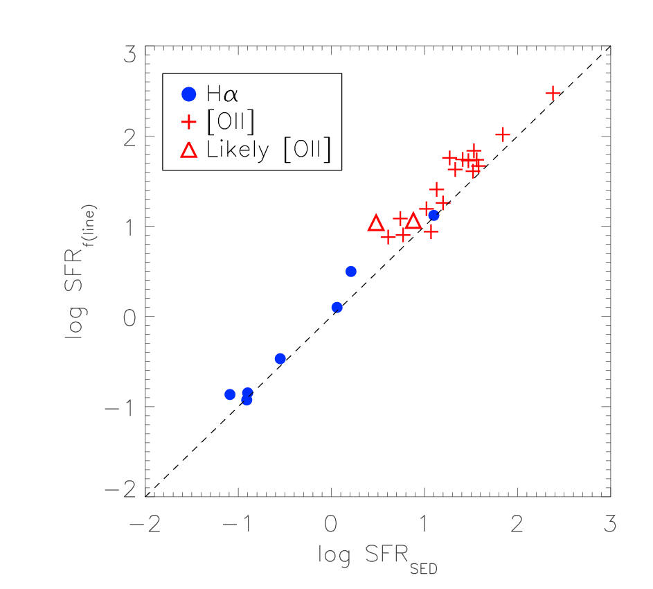
Emission lines provide us with an alternative for measuring the SFR. We correct the emission line fluxes for intrinsic reddening using the best fit E(B-V) from the LePhare fits and a Calzetti extinction curve. We then calculate and Oii luminosities which are converted to a SFR using the calibrations in Kennicutt (1998), and we include a downward correction of a factor of 1.8 to correct from a Salpeter to a Chabrier IMF. The result is shown in Fig. 14, which demonstrates that there is an excellent agreement between SFRs derived from emission lines and from the SED fits. In fact the average offset in the SFR is just dex between the two different methods. Assuming a typical Nii/H ratio of 0.1 appropriate for low-mass galaxies, the emission line fluxes and the blue points in Fig. 14 will have a downward correction of 0.05 dex. Including this correction the offset between the emission line derived SFRs and the SED SFRs is .
4.3 Clustering and large scale structure in three narrow redshift slices
In this section we consider the extended sample of 58 objects in three redshift slices. In Fig. 15 we plot the objects in the three redshift slices overlaid on our narrow band image (in black contours). In this figure we also show the masked lower signal-to-noise regions (shaded grey). The same field covers different physical scales, and different comoving scales, in the three redshift slices. In Fig. 16 we again plot the three slices separately, but here we have scaled them all to the same comoving scale. We have subsequently found that the z=1.84 cluster has been discovered independently in a study based on CANDELS and 3D-HST spectroscopic redshifts in the field (Mei et al. 2014). We refer the reader to this work for further discussion of this interesting structure.
One feature which is immediately visible is the concentration of Oii emitters in the lower left quadrant. In section 4.1 we found that the Oii emitter sample on average has higher mass than galaxies in the other slices, so because high mass galaxies are known to cluster more strongly than low mass galaxies, this is indeed the slice in which we would be most likely to find a galaxy cluster. In Fig. 16 we have marked a circle with a diameter of 2.55 comoving Mpc, which encloses 13 of the 23 Oii emitters in our extended sample. We have also marked the position of the highest mass galaxy in our sample, and it is seen to fall very close to the centre of the circle. From Fig. 15 we see that there is indeed evidence for a higher density of both optical and X-ray sources (Xue et al. 2012) around the position of the clump of Oii emitters. Computing the surface density of galaxies inside the circle we find 2.5 per comoving while outside of that it is 0.08 per comoving . On the basis of the observations reported above, we here conclude that we have identified a galaxy cluster at in our Oii redshift slice.
Simulations of early galaxy and structure formation all share a common prediction that the first structures to form are filaments who’s ends are connected in nodes. Young low mass galaxies form in the filaments, and while they assemble further and grow, they also drift along the filaments into the nodes where they form galaxy groups and eventually clusters (Monaco et al. 2005). Samples of high mass galaxies are therefore strongly clustered and well suited to identify the nodes as we showed in the previous paragraph, but in order to identify filaments one needs samples of lower mass galaxies covering volumes large enough to cover the expected sizes of filaments (20-25 Mpc), (Demiański & Doroshkevich 1999). The end product of the evolution of this cosmic web has been well studied at low redshift, and recently a large catalogue of filaments in the redshift range was published Tempel et al. (2014), but at higher redshifts than 0.155 this becomes much very difficult. Warren & Møller (1996) argued that Ly emission line selected galaxies have lower masses than continuum flux selected samples, and suggested that they could be used to identify filaments. Møller & Warren (1998) showed on a statistical basis that Ly emitters do tend to line up in strings. Nevertheless, the actual mapping of filaments is hampered by two issues: mostly the observed volumes are too small, and mostly there is no follow-up spectroscopy which is required to provide the 3-D mapping of the volume.

In one case a fully resolved filament mapped in Ly was identified at z=3.04 (Møller & Fynbo 2001) where a total of eight objects were found to be enclosed in a cylinder with proper radius 400 kpc which in the cosmology we use here corresponds to also 400 kpc. In Fig. 16 we see that 10 of 17 galaxies at lie close to a line going almost diagonally from the lower left corner of the field towards the upper right. This could be a chance alignment of galaxies at mixed redshifts, but it could also be a filament seen under some inclination angle. As in the work by Møller & Fynbo (2001) our field is too small to identify a filament which lies in the plane of the sky, we would see too few objects in such a small filament section. To test if we do indeed have enough 3-D information we have also in Fig. 16 marked (black squares) those objects in the Oiii slice for which we have spectroscopic redshifts, and we see that we have 5 spectroscopic redshifts covering the entire length of the diagonal.

In Fig. 17 we again plot the objects in the Oiii slice, but here in proper length scale, and with the redshifts of the 5 galaxies on the diagonal line marked. We see that the redshifts in general grow from the upper right towards the lower left, so this does indeed appear to be a filament pointing from the upper right towards the lower left away from us. In order to compare to the previously reported Ly filament we have marked the width (400 kpc) of that filament on top of this one by dashed red lines, and all 5 objects are seen to fit well within this cylinder in this projection. Availability of spectroscopic redshifts allow us to also compute the arrangement of the objects along the line of sight.

The Oiii redshift slice is thicker than the other two slices because we here have three individual lines (Oiii 5007, Oiii 4959, and H) either of which could fall into the narrow pass band. We visualize this in Fig. 18 where we have kept the field y-axis of Fig. 17, but have turned the volume 90 degrees and replaced the x-axis by the z-axis (i.e. redshift converted to proper distance). The three dotted boxes here represent the volumes sampled by each of the three emission lines, green dots are the galaxies, and the diagonal dashed lines again mark out a filament of thickness as in Fig. 17. We see that the first four galaxies would indeed fit into a straight, cylindrical filament of this thickness, but it would be somewhat longer than the Ly filament at redshift 3.04. The last galaxy seen in H may well belong to the same filament, but it would have to be bent or thicker in that case. The length of the filament is in excellent agreement with the detection of the Ly filament at reported by Matsuda et al. (2005) and the recent work at low redshifts Tempel et al. (2014).
In conclusion, we have shown that emission line selected galaxies at those redshifts are well suited to perform observational tests of simulations of large scale structure. The H field size is in this case too small, but surveys over larger fields like UltraVISTA (McCracken et al. 2012; Milvang-Jensen et al. 2013) will provide fields of sufficient size. The Oii slice has a larger volume, and in general the Oii selected galaxies have higher mass than the lower redshift slices, making the Oii slice ideal for rich group and cluster statistics. The Oiii slice is extremely well suited for filament searches because the depth allows to identify filaments at any inclination angle. This promises that it may soon be possible to perform the alternative and ”purely geometrical” cosmological test and determine using filaments as described in detail by Weidinger et al. (2002). Identifying filaments require spectroscopic redshifts, or some other diagnostic for more accurate redshift determination. One such novel method using only VISTA narrow band data has recently been described (Zabl et al. in preparation).
5 Discussion and conclusions
5.1 Galaxy scaling relations at low masses
Understanding the scaling relations of galaxies of all masses is fundamental to understand galaxy formation and evolution. Yet, galaxy samples selected in all emission bands ranging from X-rays over UV, optical, IR, sub-mm, and mm, to radio, all form flux limited samples of galaxies being the most luminous, and presumably the most massive, of their kind. Such samples are, by definiton, the easiest to obtain, and by right large fractions of our knowledge of high redshift galaxies originate from such samples. However, to explore the low mass range of galaxies, notably at high redshifts, other selection techniques are required. One such technique is emission line selection via deep narrow and broad band imaging.
We are involved in several narrow/broad band imaging surveys, and in this paper we have reported on a pilot project to study the feasibility of using such surveys to trace low mass galaxy scaling relations and their redshift evolution. Simple narrow/broad emission line selection allows to select galaxies with strong emission lines, thereby providing a deepening of the flux limited samples, and in this present study we have specifically chosen a broad-narrow-broad selection that results in a selection of the highest emission line equivalent width galaxies. Two simple predictions for a study of this kind would be
(i) that our sample in the mean could have higher SFR for any given galaxy stellar mass, and
(ii) that our sample in the mean will select galaxies down to lower
stellar masses than continuum flux limited samples.
We carry out a detailed
comparison of our dataset to previous studies and find that both
of those predictions have been confirmed in this work. We
thus provide an “upper boundary” to the main sequence of star formation
(MS) at each of the three redshifts we study.
Our comparison to previous work also show that the MS has a significantly steeper slope at the low mass end (below ) than at higher masses.
5.2 Narrow band selection as cosmological tool
Any narrow/broad band survey carried out at a wavelength in excess of the rest wavelength of H provides a roughly even coverage of three widely separated narrow redshift slices corresponding to the redshifted wavelengths of H, oiii/H, and oii. A few additional species at other wavelengths will also on occasion appear, but only rarely, due to the much weaker strength of their transitions. The exact ratio of detected objects between the three main slices depends on their relative equivalent widths (as a function of redshift), their relative number density (as a function of redshift), and of the ratio of the surveyed volumes (as a function of narrow band wavelength and assumed cosmology).
In this work we have surveyed comoving volumes of 1221 Mpc3 (H), 3092 Mpc3 (3 due to H, Oiii4959, and Oiii5007) and 5536 Mpc3 (Oii). Down to our conservatively chosen narrow-band AB magnitude limit of 24.8 they distribute in the following proportions: H emitters 20%, Oiii/H emitters 30% and Oii-emitters 50% (see Fig. 5). We compare our redshifts to previous photo-z redshifts from the literature and show that narrow band selection allows a much more accurate redshift assignment, notably in the highest redshift slices. The errors on redshift assignment from photo-z will propagate into errors on the physical parameters ( and SFR) so smaller, but more accurate, samples of narrow band selected galaxies will provide checks to see if the propagated errors simply add scatter, or if they add systematic effects.
We show that the galaxies can be classified fairly robustly based on two broad band colours (Fig. 6) confirming the earlier study by Bayliss et al. (2011). Therefore, we conclude that emission-line selected galaxies do indeed split into the evolutionary groups according to their color. In Fig. 10 we see that the galaxies in our lowest redshift slice on average have the lowest masses, and that galaxies then become progressively more massive at higher redshifts. This could possibly be related to the selection via different emission lines in the three slices, but is more likely a result of using the same observed magnitude limit for all slices. One very interesting thing to note is that we are able to select star forming galaxies of stellar masses down to at a redshift of 1.85, and well below that in the other two slices. With emission selected samples it is very difficult to study low mass galaxies beyond the critical redshift of ”cosmic high noon” at z=2.5, but absorption selected galaxy samples and samples selected as gamma ray burst host galaxies (GRBs) have been shown to reach much lower masses (Møller et al. (2013); Christensen et al. (2014); Arabsalmani et al. (2015)). Therefore, in order to be able to connect absorption and GRB selected samples (with median of ) with continuum emission selected samples at high redshifts, it is important to create well studied samples with a wide overlap in stellar masses. Absorption selected galaxies are in general more easily identified via line emission than via continuums emission (Weatherley et al. 2005; Rauch et al. 2008; Fynbo et al. 2010; Fynbo et al. 2011; Fynbo et al. 2013, e.g.), and the ongoing UltraVISTA (McCracken et al. 2012) narrow-band survey covering 0.8 deg2 at slightly higher redshifts (for H: z=0.815, for Oiii/H: z=1.38/1.45 and for Oii: z=2.19) will create a large sample of low mass emission line selected galaxies in those three slices (Milvang-Jensen et al. 2013). The UltraVISTA sample will be well suited to connect the current flux limited galaxy samples out to the highest redshifts (z=6-8) currently explored by DLA galaxies and GRBs.
One of the objectives of this paper is to derive more robust forecasts on and what will be found in ongoing or upcoming deep surveys, in particular the UltraVISTA survey (McCracken et al. 2012; Milvang-Jensen et al. 2013). The UltraVISTA survey uses a slightly redder narrow-band filter centered at (Milvang-Jensen et al. 2013), but this difference is sufficiently small that evolutionary effects on the population of emitters (H, oiii/H and oii) should be small. We can hence make forecasts for which numbers of the most common types of such emitters we expect to find in the UltraVISTA survey based on the present work. Scaling with the area we expect to detect 1000 of each of H, oiii, and oii emitters. Given the large area of the UltraVISTA we predict to find more rare line-emitters that are not represented in the more than 70 times smaller area sampled in the present work.
5.3 Structure formation traced by emission line selected galaxies
In Fig. 12 we show that objects in the Oii slice on average have higher masses than those of the other two slices. As argued by Møller & Fynbo (2001) and Monaco et al. (2005), the lowest mass galaxies at any redshift are the best candidates for mapping out the filamentary structure of the cosmic web, while the higher mass galaxies will be more clustered around the nodes of the web, and could hence mark the sites of early cluster formation.
In this paper we have pursued their line of thought and identified a galaxy cluster (or proto cluster) at . The cluster has an elliptical shape as predicted by N-body simulations and has no extended X-ray emission so it is probably in its early stages of formation. The galaxy with the highest mass of our entire sample lies in the centre of the forming cluster, and has been identified as an X-ray emitter. This makes this galaxy of special interest since it is a very good candidate for the pre-stage of a central cluster cD galaxy.
Secure identification of filaments is more difficult since it requires even better redshifts than the narrow band data alone can provide. We identified a possible filament lying diagonally across the field of the oiii slice, and enough of the objects had known spectroscopic redshifts for a 3D mapping. The candidate filament has width and length in good agreement with simulations, and with the previous detection of Møller & Fynbo (2001). Obtaining a few more redshifts would be good in order to securely confirm the identification, but the detection of a forming cluster and a likely filament are examples of the strong potential for tracing the formation of structure in the early universe with deep narrow band data.
Acknowledgements.
We thank Thomas Krühler and Jens Hjorth for useful suggestions. Special thanks to Olivier Ilbert for immense help with LePhare code. We thank the referee for comments that helped improve the paper. The Dark Cosmology Centre is funded by the DNRF. The research leading to these results has received funding from the European Research Council under the European Union’s Seventh Framework Program (FP7/2007-2013)/ERC Grant agreement no. EGGS-278202. BC acknowledges support from the ERC starting grant CALENDS. This research has made use of the SIMBAD database, operated at CDS, Strasbourg, France.References
- Arabsalmani et al. (2015) Arabsalmani, M., Møller, P., Fynbo, J. P. U., et al. 2015, MNRAS, 446, 990
- Arnouts et al. (1999) Arnouts, S., Cristiani, S., Moscardini, L., et al. 1999, MNRAS, 310, 540
- Balestra et al. (2010) Balestra, I., Mainieri, V., Popesso, P., et al. 2010, A&A, 512, A12
- Bayliss et al. (2011) Bayliss, K. D., McMahon, R. G., Venemans, B. P., Ryan-Weber, E. V., & Lewis, J. R. 2011, MNRAS, 413, 2883
- Brammer et al. (2008) Brammer, G. B., van Dokkum, P. G., & Coppi, P. 2008, ApJ, 686, 1503
- Brinchmann et al. (2004) Brinchmann, J., Charlot, S., White, S. D. M., et al. 2004, MNRAS, 351, 1151
- Bruzual & Charlot (2003) Bruzual, G. & Charlot, S. 2003, MNRAS, 344, 1000
- Calzetti et al. (2000) Calzetti, D., Armus, L., Bohlin, R. C., et al. 2000, ApJ, 533, 682
- Cardamone et al. (2010) Cardamone, C. N., van Dokkum, P. G., Urry, C. M., et al. 2010, ApJS, 189, 270
- Castellano et al. (2010) Castellano, M., Fontana, A., Boutsia, K., et al. 2010, A&A, 511, A20
- Castro Cerón et al. (2010) Castro Cerón, J. M., Michałowski, M. J., Hjorth, J., et al. 2010, ApJ, 721, 1919
- Chabrier (2003) Chabrier, G. 2003, PASP, 115, 763
- Christensen et al. (2004) Christensen, L., Hjorth, J., & Gorosabel, J. 2004, A&A, 425, 913
- Christensen et al. (2014) Christensen, L., Møller, P., Fynbo, J. P. U., & Zafar, T. 2014, MNRAS, 445, 225
- Christensen et al. (2012) Christensen, L., Richard, J., Hjorth, J., et al. 2012, MNRAS, 427, 1953
- Clément et al. (2012) Clément, B., Cuby, J.-G., Courbin, F., et al. 2012, A&A, 538, A66
- Daddi et al. (2007) Daddi, E., Dickinson, M., Morrison, G., et al. 2007, ApJ, 670, 156
- Demiański & Doroshkevich (1999) Demiański, M. & Doroshkevich, A. G. 1999, MNRAS, 306, 779
- Fynbo et al. (2013) Fynbo, J. P. U., Geier, S. J., Christensen, L., et al. 2013, MNRAS, 436, 361
- Fynbo et al. (2010) Fynbo, J. P. U., Laursen, P., Ledoux, C., et al. 2010, MNRAS, 408, 2128 (F10)
- Fynbo et al. (2003) Fynbo, J. P. U., Ledoux, C., Møller, P., Thomsen, B., & Burud, I. 2003, A&A, 407, 147
- Fynbo et al. (2011) Fynbo, J. P. U., Ledoux, C., Noterdaeme, P., et al. 2011, MNRAS, 413, 2481
- Giavalisco et al. (2004) Giavalisco, M., Ferguson, H. C., Koekemoer, A. M., et al. 2004, ApJ, 600, L93
- Goldoni (2011) Goldoni, P. 2011, Astronomische Nachrichten, 332, 227
- Guo et al. (2013) Guo, Y., Ferguson, H. C., Giavalisco, M., et al. 2013, ApJS, 207, 24
- Guo et al. (2012) Guo, Y., Giavalisco, M., Ferguson, H. C., Cassata, P., & Koekemoer, A. M. 2012, ApJ, 757, 120
- Hodge et al. (2013) Hodge, J. A., Karim, A., Smail, I., et al. 2013, ApJ, 768, 91
- Ilbert et al. (2006) Ilbert, O., Arnouts, S., McCracken, H. J., et al. 2006, A&A, 457, 841
- Jacobs et al. (2011) Jacobs, B. A., Sanders, D. B., Rupke, D. S. N., et al. 2011, AJ, 141, 110
- Karim et al. (2011) Karim, A., Schinnerer, E., Martínez-Sansigre, A., et al. 2011, ApJ, 730, 61
- Kennicutt (1998) Kennicutt, Jr., R. C. 1998, ARA&A, 36, 189
- Koyama et al. (2013) Koyama, Y., Smail, I., Kurk, J., et al. 2013, MNRAS, 434, 423
- Krühler et al. (2011) Krühler, T., Greiner, J., Schady, P., et al. 2011, A&A, 534, A108
- Le Fèvre et al. (2015) Le Fèvre, O., Tasca, L. A. M., Cassata, P., et al. 2015, A&A, 576, A79
- Le Fèvre et al. (2004) Le Fèvre, O., Vettolani, G., Paltani, S., et al. 2004, A&A, 428, 1043
- Le Floc’h et al. (2003) Le Floc’h, E., Duc, P.-A., Mirabel, I. F., et al. 2003, A&A, 400, 499
- Ledoux et al. (2006) Ledoux, C., Petitjean, P., Fynbo, J. P. U., Møller, P., & Srianand, R. 2006, A&A, 457, 71
- Lee et al. (2015) Lee, N., Sanders, D. B., Casey, C. M., et al. 2015, ApJ, 801, 80
- Ly et al. (2012) Ly, C., Malkan, M. A., Kashikawa, N., et al. 2012, ApJ, 757, 63
- Maiolino et al. (2008) Maiolino, R., Nagao, T., Grazian, A., et al. 2008, A&A, 488, 463
- Malhotra & Rhoads (2004) Malhotra, S. & Rhoads, J. E. 2004, ApJ, 617, L5
- Matsuda et al. (2005) Matsuda, Y., Yamada, T., Hayashino, T., et al. 2005, ApJ, 634, L125
- McCracken et al. (2012) McCracken, H. J., Milvang-Jensen, B., Dunlop, J., et al. 2012, A&A, 544, A156
- Mei et al. (2014) Mei, S., Scarlata, C., Pentericci, L., et al. 2014, ArXiv e-prints, arXiv:1403.7524
- Michałowski et al. (2010) Michałowski, M., Hjorth, J., & Watson, D. 2010, A&A, 514, A67
- Mignoli et al. (2005) Mignoli, M., Cimatti, A., Zamorani, G., et al. 2005, A&A, 437, 883
- Milvang-Jensen et al. (2013) Milvang-Jensen, B., Freudling, W., Zabl, J., et al. 2013, A&A, 560, A94
- Møller & Warren (1998) Møller, P. & Warren, S. J. 1998, MNRAS, 299, 661
- Møller et al. (2013) Møller, P., Fynbo, J. P. U., Ledoux, C., & Nilsson, K. K. 2013, MNRAS, 430, 2680
- Møller & Fynbo (2001) Møller, P. & Fynbo, J. U. 2001, A&A, 372, L57
- Møller & Warren (1993) Møller, P. & Warren, S. J. 1993, A&A, 270, 43
- Monaco et al. (2005) Monaco, P., Møller, P., Fynbo, J. P. U., et al. 2005, A&A, 440, 799
- Morris et al. (2015) Morris, A. M., Kocevski, D. D., Trump, J. R., et al. 2015, ArXiv e-prints, arXiv:1502.02659
- Nilsson et al. (2007) Nilsson, K. K., Orsi, A., Lacey, C. G., Baugh, C. M., & Thommes, E. 2007, A&A, 474, 385
- Nilsson et al. (2011) Nilsson, K. K., Östlin, G., Møller, P., et al. 2011, A&A, 529, A9
- Noeske et al. (2007) Noeske, K. G., Weiner, B. J., Faber, S. M., et al. 2007, ApJ, 660, L43
- Partridge & Peebles (1967) Partridge, R. B. & Peebles, P. J. E. 1967, ApJ, 147, 868
- Pénin et al. (2014) Pénin, A., Cuby, J.-G., Clément, B., et al. 2014, ArXiv e-prints, arXiv:1410.5558
- Pritchet & Hartwick (1987) Pritchet, C. J. & Hartwick, F. D. A. 1987, ApJ, 320, 464
- Rauch et al. (2008) Rauch, M., Haehnelt, M., Bunker, A., et al. 2008, ApJ, 681, 856
- Ravikumar et al. (2007) Ravikumar, C. D., Puech, M., Flores, H., et al. 2007, A&A, 465, 1099
- Rodrigues et al. (2008) Rodrigues, M., Hammer, F., Flores, H., et al. 2008, A&A, 492, 371
- Shapley (2011) Shapley, A. E. 2011, ARA&A, 49, 525
- Sobral et al. (2014) Sobral, D., Best, P. N., Smail, I., et al. 2014, MNRAS, 437, 3516
- Steidel et al. (2003) Steidel, C. C., Adelberger, K. L., Shapley, A. E., et al. 2003, ApJ, 592, 728
- Straughn et al. (2011) Straughn, A. N., Kuntschner, H., Kümmel, M., et al. 2011, AJ, 141, 14
- Szokoly et al. (2004) Szokoly, G. P., Bergeron, J., Hasinger, G., et al. 2004, ApJS, 155, 271
- Tempel et al. (2014) Tempel, E., Stoica, R. S., Martínez, V. J., et al. 2014, MNRAS, 438, 3465
- Trump et al. (2011) Trump, J. R., Weiner, B. J., Scarlata, C., et al. 2011, ApJ, 743, 144
- Vanzella et al. (2008) Vanzella, E., Cristiani, S., Dickinson, M., et al. 2008, A&A, 478, 83
- Vanzella et al. (2005) Vanzella, E., Cristiani, S., Dickinson, M., et al. 2005, A&A, 434, 53
- Vanzella et al. (2006) Vanzella, E., Cristiani, S., Dickinson, M., et al. 2006, A&A, 454, 423
- Vernet et al. (2011) Vernet, J., Dekker, H., D’Odorico, S., et al. 2011, A&A, 536, A105
- Villforth et al. (2012) Villforth, C., Sarajedini, V., & Koekemoer, A. 2012, MNRAS, 426, 360
- Warren & Møller (1996) Warren, S. J. & Møller, P. 1996, A&A, 311, 25
- Weatherley et al. (2005) Weatherley, S. J., Warren, S. J., Møller, P., et al. 2005, MNRAS, 358, 985
- Weidinger et al. (2002) Weidinger, M., Møller, P., Fynbo, J. P. U., Thomsen, B., & Egholm, M. P. 2002, A&A, 391, 13
- Wenger et al. (2007) Wenger, M., Oberto, A., Bonnarel, F., et al. 2007, in Astronomical Society of the Pacific Conference Series, Vol. 377, Library and Information Services in Astronomy V, ed. S. Ricketts, C. Birdie, & E. Isaksson, 197
- Whitaker et al. (2014) Whitaker, K. E., Franx, M., Leja, J., et al. 2014, ApJ, 795, 104
- Xia et al. (2011) Xia, L., Malhotra, S., Rhoads, J., et al. 2011, AJ, 141, 64
- Xu et al. (2007) Xu, C., Pirzkal, N., Malhotra, S., et al. 2007, AJ, 134, 169
- Xue et al. (2012) Xue, Y. Q., Wang, S. X., Brandt, W. N., et al. 2012, ApJ, 758, 129
References
- Arabsalmani et al. (2015) Arabsalmani, M., Møller, P., Fynbo, J. P. U., et al. 2015, MNRAS, 446, 990
- Arnouts et al. (1999) Arnouts, S., Cristiani, S., Moscardini, L., et al. 1999, MNRAS, 310, 540
- Balestra et al. (2010) Balestra, I., Mainieri, V., Popesso, P., et al. 2010, A&A, 512, A12
- Bayliss et al. (2011) Bayliss, K. D., McMahon, R. G., Venemans, B. P., Ryan-Weber, E. V., & Lewis, J. R. 2011, MNRAS, 413, 2883
- Brammer et al. (2008) Brammer, G. B., van Dokkum, P. G., & Coppi, P. 2008, ApJ, 686, 1503
- Brinchmann et al. (2004) Brinchmann, J., Charlot, S., White, S. D. M., et al. 2004, MNRAS, 351, 1151
- Bruzual & Charlot (2003) Bruzual, G. & Charlot, S. 2003, MNRAS, 344, 1000
- Calzetti et al. (2000) Calzetti, D., Armus, L., Bohlin, R. C., et al. 2000, ApJ, 533, 682
- Cardamone et al. (2010) Cardamone, C. N., van Dokkum, P. G., Urry, C. M., et al. 2010, ApJS, 189, 270
- Castellano et al. (2010) Castellano, M., Fontana, A., Boutsia, K., et al. 2010, A&A, 511, A20
- Castro Cerón et al. (2010) Castro Cerón, J. M., Michałowski, M. J., Hjorth, J., et al. 2010, ApJ, 721, 1919
- Chabrier (2003) Chabrier, G. 2003, PASP, 115, 763
- Christensen et al. (2004) Christensen, L., Hjorth, J., & Gorosabel, J. 2004, A&A, 425, 913
- Christensen et al. (2014) Christensen, L., Møller, P., Fynbo, J. P. U., & Zafar, T. 2014, MNRAS, 445, 225
- Christensen et al. (2012) Christensen, L., Richard, J., Hjorth, J., et al. 2012, MNRAS, 427, 1953
- Clément et al. (2012) Clément, B., Cuby, J.-G., Courbin, F., et al. 2012, A&A, 538, A66
- Daddi et al. (2007) Daddi, E., Dickinson, M., Morrison, G., et al. 2007, ApJ, 670, 156
- Demiański & Doroshkevich (1999) Demiański, M. & Doroshkevich, A. G. 1999, MNRAS, 306, 779
- Fynbo et al. (2013) Fynbo, J. P. U., Geier, S. J., Christensen, L., et al. 2013, MNRAS, 436, 361
- Fynbo et al. (2010) Fynbo, J. P. U., Laursen, P., Ledoux, C., et al. 2010, MNRAS, 408, 2128 (F10)
- Fynbo et al. (2003) Fynbo, J. P. U., Ledoux, C., Møller, P., Thomsen, B., & Burud, I. 2003, A&A, 407, 147
- Fynbo et al. (2011) Fynbo, J. P. U., Ledoux, C., Noterdaeme, P., et al. 2011, MNRAS, 413, 2481
- Giavalisco et al. (2004) Giavalisco, M., Ferguson, H. C., Koekemoer, A. M., et al. 2004, ApJ, 600, L93
- Goldoni (2011) Goldoni, P. 2011, Astronomische Nachrichten, 332, 227
- Guo et al. (2013) Guo, Y., Ferguson, H. C., Giavalisco, M., et al. 2013, ApJS, 207, 24
- Guo et al. (2012) Guo, Y., Giavalisco, M., Ferguson, H. C., Cassata, P., & Koekemoer, A. M. 2012, ApJ, 757, 120
- Hodge et al. (2013) Hodge, J. A., Karim, A., Smail, I., et al. 2013, ApJ, 768, 91
- Ilbert et al. (2006) Ilbert, O., Arnouts, S., McCracken, H. J., et al. 2006, A&A, 457, 841
- Jacobs et al. (2011) Jacobs, B. A., Sanders, D. B., Rupke, D. S. N., et al. 2011, AJ, 141, 110
- Karim et al. (2011) Karim, A., Schinnerer, E., Martínez-Sansigre, A., et al. 2011, ApJ, 730, 61
- Kennicutt (1998) Kennicutt, Jr., R. C. 1998, ARA&A, 36, 189
- Koyama et al. (2013) Koyama, Y., Smail, I., Kurk, J., et al. 2013, MNRAS, 434, 423
- Krühler et al. (2011) Krühler, T., Greiner, J., Schady, P., et al. 2011, A&A, 534, A108
- Le Fèvre et al. (2015) Le Fèvre, O., Tasca, L. A. M., Cassata, P., et al. 2015, A&A, 576, A79
- Le Fèvre et al. (2004) Le Fèvre, O., Vettolani, G., Paltani, S., et al. 2004, A&A, 428, 1043
- Le Floc’h et al. (2003) Le Floc’h, E., Duc, P.-A., Mirabel, I. F., et al. 2003, A&A, 400, 499
- Ledoux et al. (2006) Ledoux, C., Petitjean, P., Fynbo, J. P. U., Møller, P., & Srianand, R. 2006, A&A, 457, 71
- Lee et al. (2015) Lee, N., Sanders, D. B., Casey, C. M., et al. 2015, ApJ, 801, 80
- Ly et al. (2012) Ly, C., Malkan, M. A., Kashikawa, N., et al. 2012, ApJ, 757, 63
- Maiolino et al. (2008) Maiolino, R., Nagao, T., Grazian, A., et al. 2008, A&A, 488, 463
- Malhotra & Rhoads (2004) Malhotra, S. & Rhoads, J. E. 2004, ApJ, 617, L5
- Matsuda et al. (2005) Matsuda, Y., Yamada, T., Hayashino, T., et al. 2005, ApJ, 634, L125
- McCracken et al. (2012) McCracken, H. J., Milvang-Jensen, B., Dunlop, J., et al. 2012, A&A, 544, A156
- Mei et al. (2014) Mei, S., Scarlata, C., Pentericci, L., et al. 2014, ArXiv e-prints, arXiv:1403.7524
- Michałowski et al. (2010) Michałowski, M., Hjorth, J., & Watson, D. 2010, A&A, 514, A67
- Mignoli et al. (2005) Mignoli, M., Cimatti, A., Zamorani, G., et al. 2005, A&A, 437, 883
- Milvang-Jensen et al. (2013) Milvang-Jensen, B., Freudling, W., Zabl, J., et al. 2013, A&A, 560, A94
- Møller & Warren (1998) Møller, P. & Warren, S. J. 1998, MNRAS, 299, 661
- Møller et al. (2013) Møller, P., Fynbo, J. P. U., Ledoux, C., & Nilsson, K. K. 2013, MNRAS, 430, 2680
- Møller & Fynbo (2001) Møller, P. & Fynbo, J. U. 2001, A&A, 372, L57
- Møller & Warren (1993) Møller, P. & Warren, S. J. 1993, A&A, 270, 43
- Monaco et al. (2005) Monaco, P., Møller, P., Fynbo, J. P. U., et al. 2005, A&A, 440, 799
- Morris et al. (2015) Morris, A. M., Kocevski, D. D., Trump, J. R., et al. 2015, ArXiv e-prints, arXiv:1502.02659
- Nilsson et al. (2007) Nilsson, K. K., Orsi, A., Lacey, C. G., Baugh, C. M., & Thommes, E. 2007, A&A, 474, 385
- Nilsson et al. (2011) Nilsson, K. K., Östlin, G., Møller, P., et al. 2011, A&A, 529, A9
- Noeske et al. (2007) Noeske, K. G., Weiner, B. J., Faber, S. M., et al. 2007, ApJ, 660, L43
- Partridge & Peebles (1967) Partridge, R. B. & Peebles, P. J. E. 1967, ApJ, 147, 868
- Pénin et al. (2014) Pénin, A., Cuby, J.-G., Clément, B., et al. 2014, ArXiv e-prints, arXiv:1410.5558
- Pritchet & Hartwick (1987) Pritchet, C. J. & Hartwick, F. D. A. 1987, ApJ, 320, 464
- Rauch et al. (2008) Rauch, M., Haehnelt, M., Bunker, A., et al. 2008, ApJ, 681, 856
- Ravikumar et al. (2007) Ravikumar, C. D., Puech, M., Flores, H., et al. 2007, A&A, 465, 1099
- Rodrigues et al. (2008) Rodrigues, M., Hammer, F., Flores, H., et al. 2008, A&A, 492, 371
- Shapley (2011) Shapley, A. E. 2011, ARA&A, 49, 525
- Sobral et al. (2014) Sobral, D., Best, P. N., Smail, I., et al. 2014, MNRAS, 437, 3516
- Steidel et al. (2003) Steidel, C. C., Adelberger, K. L., Shapley, A. E., et al. 2003, ApJ, 592, 728
- Straughn et al. (2011) Straughn, A. N., Kuntschner, H., Kümmel, M., et al. 2011, AJ, 141, 14
- Szokoly et al. (2004) Szokoly, G. P., Bergeron, J., Hasinger, G., et al. 2004, ApJS, 155, 271
- Tempel et al. (2014) Tempel, E., Stoica, R. S., Martínez, V. J., et al. 2014, MNRAS, 438, 3465
- Trump et al. (2011) Trump, J. R., Weiner, B. J., Scarlata, C., et al. 2011, ApJ, 743, 144
- Vanzella et al. (2008) Vanzella, E., Cristiani, S., Dickinson, M., et al. 2008, A&A, 478, 83
- Vanzella et al. (2005) Vanzella, E., Cristiani, S., Dickinson, M., et al. 2005, A&A, 434, 53
- Vanzella et al. (2006) Vanzella, E., Cristiani, S., Dickinson, M., et al. 2006, A&A, 454, 423
- Vernet et al. (2011) Vernet, J., Dekker, H., D’Odorico, S., et al. 2011, A&A, 536, A105
- Villforth et al. (2012) Villforth, C., Sarajedini, V., & Koekemoer, A. 2012, MNRAS, 426, 360
- Warren & Møller (1996) Warren, S. J. & Møller, P. 1996, A&A, 311, 25
- Weatherley et al. (2005) Weatherley, S. J., Warren, S. J., Møller, P., et al. 2005, MNRAS, 358, 985
- Weidinger et al. (2002) Weidinger, M., Møller, P., Fynbo, J. P. U., Thomsen, B., & Egholm, M. P. 2002, A&A, 391, 13
- Wenger et al. (2007) Wenger, M., Oberto, A., Bonnarel, F., et al. 2007, in Astronomical Society of the Pacific Conference Series, Vol. 377, Library and Information Services in Astronomy V, ed. S. Ricketts, C. Birdie, & E. Isaksson, 197
- Whitaker et al. (2014) Whitaker, K. E., Franx, M., Leja, J., et al. 2014, ApJ, 795, 104
- Xia et al. (2011) Xia, L., Malhotra, S., Rhoads, J., et al. 2011, AJ, 141, 64
- Xu et al. (2007) Xu, C., Pirzkal, N., Malhotra, S., et al. 2007, AJ, 134, 169
- Xue et al. (2012) Xue, Y. Q., Wang, S. X., Brandt, W. N., et al. 2012, ApJ, 758, 129
Appendix A Thumbnail images for the ”Basic Sample” galaxies


