We introduce a new clustering of active regions that is based on the local geometry observed in Line of Sight magnetogram and continuum images. We use a reduced-dimension representation of an active region that is obtained by factoring the corresponding data matrix comprised of local image patches. Two factorizations can be compared via the definition of appropriate metrics on the resulting factors. The distances obtained from these metrics are then used to cluster the active regions. We find that these metrics result in natural clusterings of active regions. The clusterings are related to large scale descriptors of an active region such as its size, its local magnetic field distribution, and its complexity as measured by the Mount Wilson classification scheme. We also find that including data focused on the neutral line of an active region can result in an increased correspondence between our clustering results and other active region descriptors such as the Mount Wilson classifications and the value. Matrix factorization of image patches is a promising new way of characterizing active regions. We provide some recommendations for which metrics, matrix factorization techniques, and regions of interest to use to study active regions.
Image patch analysis of sunspots and active regions. II. Clustering via matrix factorization
Abstract
Separating active regions that are quiet from potentially eruptive ones is a key issue in Space Weather applications. Traditional classification schemes such as Mount Wilson and McIntosh have been effective in relating an active region large scale magnetic configuration to its ability to produce eruptive events. However, their qualitative nature prevents systematic studies of an active region’s evolution for example.
keywords
Sun – active region – sunspot – neutral line – data analysis – classification – clustering – image patches – Hellinger distance – Grassmannian1 Introduction
1.1 Context
Identifying properties of active regions (AR) that are necessary and sufficient for the production of energetic events such as solar flares is one of the key issues in space weather. The Mount Wilson classification (see Table 1 for a brief description of its four main classes) has been effective in relating a sunspot’s large scale magnetic configuration with its ability to produce flares. Künzel (1960) pointed out the first clear connection between flare productivity and magnetic structure, and introduced a new magnetic classification, , to supplement Hale’s , and classes (Hale et al., 1919). Several studies showed that a large proportion of all major flare events begin with a configuration (Warwick, 1966; Mayfield and Lawrence, 1985; Sammis et al., 2000).
| Class | Classification Rule | Number of AR | Number of Patches |
| A single dominant spot | 50 | 13,358 | |
| A pair of dominant spots of opposite polarity | 192 | 75,463 | |
| A sunspot where a single north-south polarity | 130 | 95,631 | |
| inversion line cannot divide the two polarities | |||
| A sunspot where umbrae of opposite polarity | 52 | 66,195 | |
| are together in a single penumbra |
The categorical nature of the Mount Wilson classification, however, prevents the differentiation between two sunspots with the same classification and makes the study of an AR’s evolution cumbersome. Moreover, the Mount Wilson classification is generally carried out manually which results in human bias. Several papers (Stenning et al., 2013; Colak and Qahwaji, 2008; Colak and Qahwaji, 2009) have used supervised techniques to reproduce the Mount Wilson and other schemes which has resulted in a reduction in human bias.
To go beyond categorical classification in the flare prediction problem, the last decade has seen many efforts in describing the photospheric magnetic configuration in more details. Typically, a set of scalar properties is derived from line of sight (LOS) or vector magnetogram and analyzed in a supervised classification context to derive which combination of properties is predictive of increased flaring activity (Leka and Barnes, 2004; Guo et al., 2006; Schrijver, 2007; Barnes et al., 2007; Georgoulis and Rust, 2007; Falconer et al., 2008; Song et al., 2009; Huang et al., 2010; Yu et al., 2010; Ahmed et al., 2011; Lee et al., 2012; Bobra and Couvidat, 2015). Examples of scalar properties include: sunspot area, total unsigned magnetic flux, flux imbalance, neutral line length, maximum gradients along the neutral line, or other proxies for magnetic connectivity within ARs. These scalar properties are features that can be used as input in flare prediction. However, there is no guarantee that these selected features exploit the information present in the data in an optimal way for the flare prediction problem.
1.2 Contribution
We introduce a new data-driven method to cluster ARs using information contained in magnetogram and continuum. Instead of focusing on the best set of properties that summarizes the information contained in those images, we study the natural geometry present in the data via a reduced-dimension representation of such images. The reduced-dimension is implemented via matrix factorization of an image patch representation as explained in Section 1.3. We show how this geometry can be used for classifying ARs in an unsupervised way, that is, without including AR labels as input to the analysis.
We consider the same dataset as in Moon et al. (2015). It is obtained from the Michelson Doppler Imager (MDI) instrument (Scherrer et al., 1995) on board the SOHO Spacecraft. SOHO-MDI provides two to four times per day a white-light continuum image observed in the vicinity of the Ni i 676.7L nm photospheric absorption line. MDI LOS magnetograms are recorded with a higher nominal cadence of 96 minutes. We selected 424 sunspot images within the time range of 1996-2010. They span the various Mount Wilson classifications (see Table 1), are located within of central meridian, and have corresponding observations in both MDI continuum and MDI LOS magnetogram. We use level 1.8 data for both modalities.

Our method can be adapted to any definition of the support of an AR, or Region of Interest (ROI), and such ROI must be given a priori. We consider three types of ROIs:
- 1.
Umbrae and penumbrae masks obtained with the Sunspot Tracking and Recognition Algorithm (STARA) (Watson et al., 2011) from continuum images. These sunspot masks encompass the regions of highest variation observed in both continuum and magnetogram images, and hence are used primarily to illustrate our method. Figure 1 provides some examples of AR images overlaid with their respective STARA masks.
- 2.
The neutral line region, defined as the set of pixels situated no more than 10 pixels (20 arcsec) away from the neutral line, and located within the Solar Monitor Active Region Tracker (SMART) masks (Higgins et al., 2011), which defines magnetic AR boundaries.
- 3.
The set of pixels that are used as support for the computation of the -value defined in Schrijver (2007). The -value measures a weighted absolute magnetic flux, where the weights are positive only around the neutral line.
Our patch-based matrix factorization method investigates the fine scale structures encoded by localized gradients of various directions and amplitudes, or locally smooth areas for example. In contrast, the Mount Wilson classification encodes the relative locations and sizes of concentrations of opposite polarity magnetic flux on a large scale. Although both classification schemes rely on completely different methods, using the first ROI defined above, we find some similarities (see Section 5). Moreover the Mount Wilson classification can guide us in the interpretation of the results and clusters obtained.
The shape of the neutral line separating the two main polarities in an AR is a key element in the Mount Wilson classification scheme, and the magnetic field gradients observed along the neutral line are important information in the quest for solar activity prediction (Schrijver, 2007; Falconer et al., 2008). We therefore analyze the effect of including the neutral line region in Section 5.
Results based on the third ROI are compared directly to the -value. The various comparisons enable us to evaluate the potential of our method for flare prediction.
1.3 Reduced dimension via matrix factorization
Our data-driven method is based on a reduced-dimension representation of an AR ROI via matrix factorization of image patches. Matrix factorization is a widely used tool to reveal patterns in high dimensional datasets. Applications outside of solar physics are numerous and range e.g. from multimedia activity correlation, neuroscience, gene expression (Bazot et al., 2013), to hyperspectral imaging (Mittelman et al., 2012).
The idea is to express a multivariate observation as a linear combination of a reduced number of components , each weighted by some (possibly random) coefficients :
| (1) |
where represents residual noise. With , the equivalent matrix factorization representation is written as
| (2) |
where is a data matrix containing observations of different variables, is the matrix containing the ‘dictionary elements’ (called ’factor loadings’ in some applications) and is the matrix of coefficients (or ‘factor scores’). The matrix contains residuals from the matrix factorization model fitting. Finding and from the knowledge of alone is a severely ill-posed problem, hence prior knowledge is needed to constrain the solution to be unique.
Principal Component Analysis (PCA) (Jolliffe, 2002) is probably the most widely used dimensionality reduction technique. It seeks principal directions that capture the highest variance in the data under the constraints that these directions are mutually orthogonal, thereby defining a subspace of the initial space that exhibit information rather than noise. The PCA solution can be written as a matrix factorization thanks to the Singular Value Decomposition (SVD) (Moon and Stirling, 2000), and so we use SVD in the clustering method presented here.
The Nonnegative Matrix Factorization (NMF) (Lee and Seung, 2001) is also considered in this paper. Instead of imposing orthogonality, it constrains elements of matrices and to be nonnegative. We further impose that each column of has elements that sum up to one, thereby effectively using a formulation identical to one used in hyperspectral unmixing (Bioucas-Dias et al., 2012).
Unmixing techniques exploit the high redundancy observed in similar bandpasses. They aim at separating the various contributions and at estimating a smaller set of less dependent source images. Matrix factorization, known as ‘blind source separation’ in this context, has many applications, ranging from biomedical imaging, chemometrics, to remote sensing (Comon and Jutten, 2010), and recently to the extraction of salient morphological features from multi-wavelength extreme ultraviolet solar images (Dudok de Wit et al., 2013).
In this paper, we wish to factorize a data matrix containing observations of different variables as in Equation (2) where the dictionary matrix spans a subspace of the initial space, with . We consider the cases where is formed from a single image as well as from multiple images.
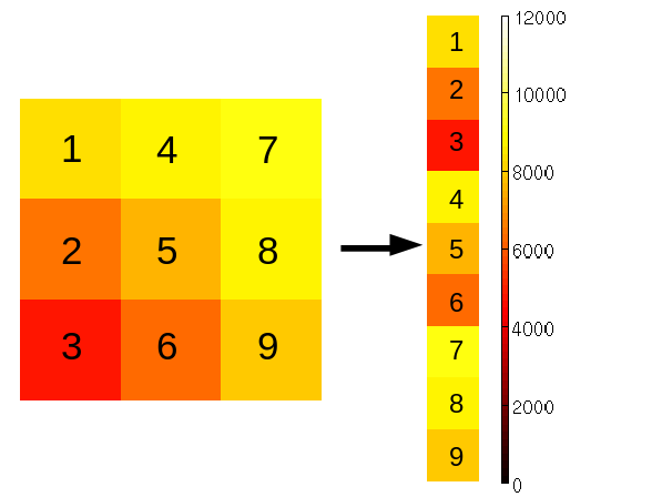
When a single image is used, the data matrix is built from a pixel image by taking overlapping -pixel neighborhoods called patches. Figure 2 (left) presents such a patch and its column representation. The rows of the th column of are thus given by the pixel values in the neighborhood of pixel . The right plot in Figure 2 provides the number of patches in each pair of AR images when using the STARA masks. When multiple images are used, such as when analyzing collectively all images from a given Mount Wilson class, the patches are combined into a single data matrix. Table 1 gives the total number of patches from each Mount Wilson class when using the STARA masks.
A factorization of a data matrix containing image patches is illustrated in Figure 3. In this figure, let be the first column of , containing the intensity values for the first patch. These intensity values are decomposed as a sum of elements as in Equation (1) where is the th column of and is the th element of . In this representation, the vectors are the elementary building blocks common to all patches, whereas the are the coefficients specific to the first patch.


To compare ARs and cluster them based on this reduced dimension representation, some form of distance is required. To measure the distance between two ARs, we apply some metrics to the corresponding matrices or obtained from the factorizations of the two ARs. These distances are further introduced into a clustering algorithm that groups ARs based on the similarity of their patch geometry.
This paper builds upon results obtained in Moon et al. (2015), which can be summarized as follows:
- 1.
Continuum and magnetogram modalities are correlated, and there may be some advantage in considering both of them in an analysis.
- 2.
A patch size of includes a significant portion of spatial correlations present in continuum and magnetogram images.
- 3.
Linear methods for dimensionality reduction (e.g. matrix factorization) are appropriate to analyze ARs observed with continuum images and magnetogram.
With an AR area equal to pixels and an patch, the corresponding continuum data matrix and magnetogram data matrix each have size . The full data matrix considered is with size in our case. The images extracted from both modalities are normalized prior to analysis. An intrinsic dimension analysis in Moon et al. (2015) showed further that a sunspot can be represented accurately with a dictionary containing six elements.
1.4 Outline
Section 2 describes two matrix factorization methods: the singular value decomposition (SVD) and nonnegative matrix factorization (NMF). While more sophisticated methods exist that may lead to improved performance, we focus on SVD and NMF to demonstrate the utility of an analysis of a reduced dimension representation of image patches for this problem. Future work will include further refinement in the choice of matrix factorization techniques. To compare the results from this factorization we need a metric, and so we use the Hellinger distance for this purpose. To obtain some insight on how these factorizations separate the data, we make some general comparisons in Section 3. In particular, with the defined metric, we compute the pairwise distances between Mount Wilson classes to identify which classes are most similar or dissimilar according to the matrix factorization results.
Section 4 describes the clustering procedures that take the metrics’ output as input. The method called ‘Evidence Accumulating Clustering with Dual rooted Prim tree Cuts’ (EAC-DC) was introduced by Galluccio et al. (2013) and is used to cluster the ARs. By combining the two matrix factorization methods, a total of two procedures are used to analyze the data. Besides analyzing the whole sunspot data, we also look at information contained in patches situated along the neutral lines. The results of the clustering analyses are provided in Section 5.
This paper improves and extends the work in Moon et al. (2014), where fixed size square pixel regions centered on the sunspot group were used as the ROI for the matrix factorization prior to clustering. Moreover, here we are using more appropriate metrics to compare the factorization results.
2 Matrix Factorization
The intrinsic dimension analysis in Moon et al. (2015) showed that linear methods (e.g. matrix factorization) are sufficient to represent the data, and hence we focus on those. Matrix factorization methods aim at finding a set of basis vectors or dictionary elements such that each data point (in our case, pair of pixel patches) can be accurately expressed as a linear combination of the dictionary elements. Mathematically, if we use patches then this can be expressed as , where is the data matrix with data points being considered, is the dictionary with the columns corresponding to the dictionary elements, and is the matrix of coefficients. The goal is to find matrices and whose product nearly approximates . The degree of approximation is typically measured by the squared error , where denotes the Frobenius norm (Yaghoobi et al., 2009). Additional assumptions on the structure of the matrices and can be applied in matrix factorization depending on the application. Examples include assumptions of orthonormality of the columns of the dictionary , sparsity of the coefficient matrix (Ramírez and Sapiro, 2012), and nonnegativity on and (Lin, 2007).
We consider two popular matrix factorization methods: the singular value decomposition (SVD) and nonnegative matrix factorization (NMF).
2.1 Factorization using SVD
To perform matrix factorization using SVD, we take the singular value decomposition of the data matrix where is the matrix of the left singular vectors, is a diagonal matrix containing the singular values, and is a matrix of the right singular vectors. If the size of the dictionary is fixed and is less than , then the matrix of rank that is closest to in terms of the Frobenius norm is the matrix product , where and are matrices containing only the first singular vectors and contains only the first singular values (Moon and Stirling, 2000). Thus for SVD, the dictionary and coefficient matrices are and , respectively. Note that SVD enforces orthonormality on the columns of . Further details are included in Appendix A.1.
The intrinsic dimension estimated in Moon et al. (2015) determines the number of parameters required to accurately represent the data. It is used to provide an initial estimate for the size of the dictionaries . For SVD, we choose to be one standard deviation above the mean intrinsic dimension estimate, that is, or 6. The choice of is then further refined by a comparison of dictionaries in Section 3. See Section 4.2 for more on selecting the dictionary size.
Figure 4 shows the learned dictionaries using SVD on the entire data set of 424 image pairs of ARs. Interestingly, the SVD seems to consider the continuum and magnetogram separately as the magnetogram elements are essentially zero when the continuum elements are not and vice versa. This is likely caused by the orthonormality constraint. The dictionary patches largely consist of a mix of uniform patches and patches with gradients in varied directions. The second dictionary element is associated with the average magnetic field value of a patch.

2.2 Factorization using NMF
Non-negative matrix factorization (NMF) (Lee and Seung, 2001) solves the problem of minimizing while constraining and to have nonnegative values. Thus NMF is a good choice for matrix factorization when the data is nonnegative. For our problem, the continuum data is nonnegative while the magnetogram data is not. Therefore we use a modified version of NMF using projected gradient where we only constrain the parts of corresponding to the continuum to be nonnegative. An effect of using this modified version of NMF is that since the coefficient matrix is still constrained to be nonnegative, we require separate dictionary elements that are either positive or negative in the magnetogram component. Thus we use approximately 1.5 times more dictionary elements for NMF than SVD.
Since we apply NMF to the full data matrix , this enforces a coupling between the two modalities by forcing the use of the same coefficient matrix to reconstruct the matrices and . This is similar to coupled NMF which has been used in applications such as hyperspectral and multispectral data fusion (Yokoya et al., 2012).
Figure 5 shows the learned dictionary elements using NMF on the entire dataset. For NMF, the modalities are not treated separately as in the SVD results. But as for SVD, the patches largely consist of a mix of uniform patches and patches with gradients in varied directions.

2.3 SVD vs. NMF
There are advantages to both SVD and NMF matrix factorization methods which are summarized in Table 2. SVD produces the optimal rank approximation of , is fast and unique, and results in orthogonal elements (Langville et al., 2006). NMF has the advantages of nonnegativity, sparsity, and interpretability. The interpretability comes from the additive parts-based representation inherent in NMF (Langville et al., 2006). In contrast, the SVD results are not sparse which can make interpretation more difficult. However, NMF is not as robust as SVD as the NMF algorithm is a numerical approximation to a non-convex optimization problem having local minima. Thus the solution provided by the NMF algorithm depends on the initialization. More details on matrix factorization using NMF and SVD are included in Appendix A.1.
| SVD Advantages | NMF Advantages |
|---|---|
| Optimal rank approximation | Results are nonnegative |
| Fast to compute | Results are sparse |
| Unique | Sparsity and nonnegativity lead to improved interpretability |
2.4 Methods for Comparing Matrix Factorization Results
To compare the results from matrix factorization, we primarily seek a difference between the coefficients from . To aid us in choosing a dictionary size , we also require a measure of difference between dictionaries . We use the Hellinger distance and Grassmannian projection metric to measure the respective differences.
In Moon et al. (2014), the Frobenius norm was used to compare the dictionaries. However, this fails to take into account the fact that two dictionaries may have the same elements but in a different order. In this case, the Frobenius norm of the difference between two dictionaries may be high even though the dictionaries span the same subspace. A better way to measure the difference would be to compare the subspaces spanned by the dictionaries. The Grassmannian is a space which parameterizes all linear subspaces with dimension of a vector space . As an example, the Grassmannian is the space of planes through the origin of the standard Euclidean vector space in . In our case, we are concerned with the Grassmannian , where is the size of the dictionary. The space spanned by a given dictionary is then a single point in . Several metrics have been defined on this space including the Grassmannian projection metric (Stewart, 1973; Edelman et al., 1998). It can be defined as
where is the projection matrix of and is the norm. This metric is invariant to the order of the dictionary elements and compares the subspaces spanned by the dictionaries. This metric has a maximum value of 1.
To compare the coefficient matrices, we assume that the 18-dimensional pixel patches within an AR are samples from an 18-dimensional probability distribution, and that each AR has a corresponding (potentially unique) probability distribution of pixel patches. We project these samples onto a lower dimensional space by matrix factorization. In other words, we learn a dictionary and the coefficient matrix for the entire dataset , and then separate the coefficients in according to the different ARs (or groups of ARs) considered: . The columns of are a collection of projected, low-dimensionality, samples from the th AR (or group), and we let denote the corresponding probability density function. Given two such collections, we can estimate the difference between their probability distributions by estimating the information divergence. Many kinds of divergences exist such as the popular Kullback-Leibler divergence (Kullback and Leibler, 1951). We use the Hellinger distance which is defined as (Hellinger, 1909; Bhattacharyya, 1946; Csiszar, 1967)
where and are the two probability densities being compared. The Hellinger distance has the advantage over other divergences of being a metric which is not true of divergences in general. To estimate the Hellinger distance, we use the nonparametric estimator derived in Moon and Hero III (2014a); Moon and Hero III (2014b) that is based on the -nearest neighbor density estimators for the densities and . This estimator is simple to implement and achieves the parametric convergence rate when the densities are sufficiently smooth.
3 Comparisons of General Matrix Factorization Results
We apply the metrics mentioned in Section 2.4 and compare the local features as extracted by matrix factorization per Mount Wilson class. One motivation for these comparisons is to investigate differences between the Mount Wilson classes based on the Hellinger distance. Another motivation is to further refine our choice of dictionary size in preparation for clustering the ARs. When comparing the dictionary coefficients using the Hellinger distance, we want a single, representative dictionary that is able to accurately reconstruct all of the images. Then the ARs will be differentiated based on their respective distributions of dictionary coefficients instead of the accuracy of their reconstructions. The coefficient distributions can then be compared to interpret the clustering results as is done in Section 5.1.
Recall that our goal is to use unsupervised methods to separate the data based on the natural geometry. Our goal is not to replicate the Mount Wilson results. Instead we use the Mount Wilson labels in this section as a vehicle for interpreting the results.
3.1 Grassmannian Metric Comparisons
We first learn dictionaries for each of the Mount Wilson types by applying matrix factorization to a subset of the patches corresponding to sunspot groups of the respective type. We then use the Grassmannian metric to compare the dictionaries. For example, if we want to compare the and groups, we collect a subset of patches from all ARs designated as groups into a single data matrix . We then factor this matrix with the chosen method to obtain . Similarly, we obtain and then calculate .
The reason we use only a subset of patches is that each AR type has a different number of total patches (see Table 1) which may introduce bias in the comparisons. One source of potential bias in this case is due to the potentially increased patch variability in groups with more patches, which would result in increased difficulty in characterizing certain homogeneities of the patch features. This is mitigated somewhat by the fact that the local intrinsic dimension is typically less than 6 (Moon et al., 2015). However, it is possible that there may be different local subspaces with the same dimension. A second source of potential bias is in the different levels of variance of the estimates due to difference in patch numbers. To circumvent these potential biases, we use the same number of patches in each group for each comparison. For the inter-class comparison, we randomly take 13,358 patches (the number of patches in the smallest class) from each class to learn the dictionary, and then calculate the Grassmannian metric. For the intra-class comparison, we take two disjoint subsets of 6,679 patches (half the number of patches in the smallest class) from each class to learn the dictionaries. This process is repeated 100 times and the resulting mean and standard deviation are reported.
| SVD, Pooled Grassmannian, | ||||
|---|---|---|---|---|
| SVD, Pooled Grassmannian, | ||||
|---|---|---|---|---|
| NMF, Pooled Grassmannian, | ||||
|---|---|---|---|---|
| NMF, Pooled Grassmannian, | ||||
|---|---|---|---|---|
Table 3 shows the corresponding average Grassmannian distance metrics when using SVD and NMF and for different sizes of dictionaries . For SVD, the results are very sensitive to . Choosing results in large differences between the different dictionaries but for , the dictionaries are very similar. This suggests that for SVD, 6 principal components are sufficient to accurately represent the subspace upon which the sunspot patches lie. This is consistent with the results of Moon et al. (2015) where the intrinsic dimension is found to be less than 6 for most patches.
Interestingly, for the SVD results, the group is the most dissimilar to the other groups while being relatively similar to itself. In contrast, the group is fairly dissimilar to itself and relatively similar to the and groups.
The NMF results are less sensitive to . The average difference between the dictionaries and its standard deviation is larger when compared to when . However, for a given , all of the mean differences are within a standard deviation of each other. Thus on aggregate, the NMF dictionaries learned from large collections of patches from multiple images differ from each other to the same degree regardless of the Mount Wilson type.
3.2 Hellinger Distance Comparisons
For the Hellinger distance, we learn a dictionary and the coefficient matrix for the entire data set . We then separate the coefficients in according to the Mount Wilson type and compare the coefficients’ distributions using the Hellinger distance. For example, suppose that the data matrix is arranged as . This is factored as . To compare the and groups, we assume that the columns in are samples from the distribution and similarly contains samples from the distribution . We then estimate the Hellinger distance using the divergence estimator in Moon and Hero III (2014a).
When the Hellinger distance is used to compare the collections of dictionary coefficients within the sunspots, the groups are very similar, especially when using SVD (Table 4). This indicates that when the coefficients of all ARs from one class are grouped together, the distribution looks similar to the distribution of the other classes. However, there are some small differences. First the intraclass distances are often much smaller than the interclass distances which indicates that there is some relative difference between most classes. Second, for both matrix factorization methods, the groups are the most dissimilar. This could be due to the presence of a spot configuration, where umbrae of opposite polarities are within a single penumbra. Such a configuration may require specific linear combinations of the dictionary elements as compared to the other classes. The presence and absence of these linear combinations in two Mount Wilson types would result in a higher Hellinger distance between them.
| SVD, Pooled Hellinger | ||||
|---|---|---|---|---|
| 0 | 0 | 0.03 | ||
| 0.01 | 0.08 | |||
| 0.05 | ||||
| NMF, Pooled Hellinger | ||||
|---|---|---|---|---|
| 0.08 | 0.05 | 0.10 | ||
| 0.03 | 0.12 | |||
| 0.11 | ||||
Again, for clustering, we compute the pairwise Hellinger distance between each AR’s collection of coefficients. This is done by forming the data matrix from the 424 ARs as and factoring it as . The columns of are samples from a distribution and the distributions and are compared by estimating . The corresponding dictionaries for the two methods are shown in Figures 4 and 5.
Table 5 gives the average pairwise Hellinger distance between the ARs. The average distances differ more with the NMF based coefficients resulting in larger dissimilarity. The average distance is smallest when comparing the groups to all others and largest when comparing the groups to the rest. The standard deviation is also larger when comparing and groups. This may be partially related to the variability in estimation due to smaller sample sizes as the and groups contain more of the smaller ARs (see Figure 2). Overall, the average distances show that there are clear differences between the ARs within the sunspots using this metric.
| SVD, Average Hellinger | ||||
|---|---|---|---|---|
| NMF, Average Hellinger | ||||
|---|---|---|---|---|
4 Clustering of Active Regions: Methods
4.1 Clustering Algorithm
The clustering algorithm we use is the Evidence Accumulating Clustering with Dual rooted Prim tree Cuts (EAC-DC) method in Galluccio et al. (2013) which scales well for clustering in high dimensions. EAC-DC clusters the data by defining a metric based on the growth of two minimal spanning trees (MST) grown sequentially from a pair of points. To grow the MSTs, a base dissimilarity measure is required as input such as the Hellinger distance described in Section 2.4. From the new metric defined using the MSTs, a similarity measure between inputs is created. It is fed into a spectral clustering algorithm that groups together inputs which are most similar. The similarity measure based on the MSTs adapts to the geometry of the data, and this results in a clustering method that is robust and competitive with other algorithms (Galluccio et al., 2013). See Appendix A.2 for more details.
4.2 Clustering Input: Dictionary Sizes
As input to the clustering algorithm, we use the matrix factorization results as described in Section 2.4. We learn a single dictionary from the entire dataset. We then project the data onto a lower dimensional space, i.e. we learn the coefficient matrices . These matrices are the inputs in this method and the base dissimilarity measure is the Hellinger distance estimated using each AR’s respective coefficients. Table 6 provides a summary of the various dissimilarity and similarity measures that we use.
| Measure | Type | Properties |
|---|---|---|
| Grassmannian metric | Dissimilarity | Compares dictionaries by comparing the subspace |
| spanned by the dictionary elements | ||
| Hellinger distance | Dissimilarity | Compares the underlying distributions of dictionary |
| coefficients; estimated using Moon and Hero III (2014a) | ||
| EAC-DC based measure | Similarity | Based on sequentially grown MSTs of the data; |
| requires a base dissimilarity measure as input |
As mentioned in Section 2, the estimated intrinsic dimension from Moon et al. (2015) is used to provide an initial estimate for the size of the dictionaries . The choice of is further refined by the dictionary comparison results from Section 3 . For SVD, we choose to be one standard deviation above the mean intrinsic dimension estimate which is approximately 5 or 6. When comparing the dictionary coefficients, we want the single dictionary to accurately represent the images. The dictionary should not be too large as this may add spurious dictionary elements due to the noise. The results in Table 3 suggest that for SVD, the dictionaries are essentially identical for This means that dictionary elements are sufficient to accurately reconstruct most of the images. This is consistent with the intrinsic dimension estimates in Moon et al. (2015). Thus we choose when using the Hellinger distance for the SVD dictionary coefficients.
Since our mixed version of NMF requires approximately 1.5 times the number of dictionary elements as SVD (see Section 2.1), we choose within the sunspots. Since the differences between classes were similar for and , choosing strikes a balance between accurate representation of the data and limiting the effects of noise.
4.3 Clustering Input: Patches within Sunspots and Along the Neutral Line
Our main focus up to this point in this paper has been on data matrices containing the patches within the STARA masks, that is, within sunspots. The clustering based on these patches is discussed in Sections 5.1-5.2.
It is well-known, however, that the shape of the neutral line separating the main polarities plays an important role in the Mount Wilson classification. For this reason, we conduct two experiments involving data from along the neutral line.
The results of the first experiment are in Section 5.3 where we apply matrix factorization on a data matrix containing only the patches situated along the neutral line using the same ARs as in Sections 5.1-5.2. To compute the location of a neutral line in this experiment, we assume it is situated in the middle between regions of opposite polarity, and proceed as follows. First, we determine regions of high magnetic flux of each polarity using an absolute threshold at 50 Gauss. Second, we compute for each pixel the distance to the closest high flux region in each polarity using the Fast Marching method (Sethian, 1995). Once the two distance fields (one for each polarity) are calculated, the neutral line can be obtained by finding the pixels that lie on or are close to the zero level set of the difference of these two distance fields. In this paper, we choose a maximum distance of 10 pixels to determine the neutral line region.
We extract the patches that lie in the neutral line region and within the SMART mask associated to the AR. Call the resulting data matrix . We then apply SVD or NMF matrix factorization as before and calculate the pairwise distance between each AR neutral line using the Hellinger distance on the results. Define the resulting dissimilarity matrix as for whichever factorization method we are currently using. Similarly, define and as the respective data matrix and dissimilarity matrix of the data from within the sunspots using the same configuration. The base dissimilarity measure inputted in the clustering algorithm is now a weighted average of the distances computed within the neutral line regions and within the sunspots: where . Using a variety of weights, we then compare the clustering output to different labeling schemes based on the Mount Wilson labels as shown in Table 7.
| # of clusters | Mount Wilson Comparison |
|---|---|
| 2 | Simple ( and ), complex ( and ) |
| 3 | , , and complex |
| 4 | Mount Wilson (, , , and ) |
For the second experiment, we perform clustering on a ROI that selects pixels along a strong field polarity reversal line. The high gradients near strong field polarity reversal lines in LOS magnetograms are a proxy for the presence of near-photospheric electrical currents, and thus might be indicative of a non-potential configuration (Schrijver, 2007). To compute this ROI, the magnetograms are first reprojected using an equal-area, sinusoidal re-projection that uses Singular-Value Padding (DeForest, 2004). The latter is known to be more accurate than image interpolation on transformed coordinates. To conserve flux, the magnetograms are also area-normalized.
In the reprojected magnetograms, we delimit an AR using sunspot information from the Debrecen catalog (Győri et al., 2010) to obtain the location of all the pixels that belong to the spots related to an AR (called "Debrecen spots" hereafter). The ROI consists of a binary array constructed as follows:
- 1.
The pixels that belong to the Debrecen spots are assigned the scalar value 1 and all others are assigned the scalar value -1.
- 2.
From this two-valued array, we retrieve the distances from the zero level-set using a fast marching method (Sethian, 1995) implemented in the Python SciKits’ module "scikit-fmm".
- 3.
We mask out the pixels within a distance of 80 pixels from the zero level-set (in the equal-area-reprojected coordinate system).
- 4.
The ROI is delimited by the convex hull of the resulting mask, that is, the smallest convex polygon that surrounds all 1-valued pixels. The resulting mask is a binary array with the pixels inside the convex hull set to True.
Within the ROI, the -value is calculated similarly to the method described in Schrijver (2007). We dilate the image using a dilation factor of 3 pixels, and extract the flux using overlapping Gaussian masks with . Integrating the non-zero values outputs the -value, i.e, the total flux in the vicinity of the polarity-inversion line.
We then perform an image patch analysis using image patches from this region. We do this by using either SVD or NMF to do dimensionality reduction on the patches, and then estimate the Hellinger distance between ARs using the reduced dimension representation. We exclude groups from the analysis as they do not have a strong field polarity reversal line. This leaves 420 images to be clustered. The clustering assignments are then compared to the calculated value via the correlation coefficient. The results are presented in Section 5.4.
5 Clustering of Active Regions: Results
Given the choices of matrix factorization techniques (NMF and SVD) we have two different clustering results on the data. Section 5.1 focuses on the clusterings using data from within the sunspots, and Section 5.2 provides some recommendations for which metrics and matrix factorization techniques to use to study different ARs. The neutral line clustering results are then given in Section 5.3 followed by the value based experiment in Section 5.4.
5.1 Clustering within the Sunspot
We now present the clustering results when using the Hellinger distance as the base dissimilarity. The corresponding dictionary elements to the coefficients are represented in Figure 4 (for the SVD factorization) and in Figure 5 (for the NMF).
The EAC-DC algorithm does not automatically choose the number of clusters. We use the mean silhouette heuristic to determine the most natural number of clusters as a function of the data (Rousseeuw, 1987). The silhouette is a measure of how well a data point belongs to its assigned cluster. The heuristic chooses the number of clusters that results in the maximum mean silhouette. In both clustering configurations, the number of clusters that maximizes the mean silhouette is 2 so we focus on the two clustering case for all clustering schemes throughout.
To compare the clustering correspondence, we use the adjusted Rand index (ARI). The ARI is a measure of similarity between two clusterings (or a clustering and labels) and takes values between -1 and 1. A 1 indicates perfect agreement between the clusterings and a 0 corresponds to the agreement from a random assignment (Rand, 1971). Thus a positive ARI indicates that the clustering correspondence is better than a random clustering while a negative ARI indicates it is worse. The ARI between the NMF and SVD clusterings is which indicates some overlap.
Visualizing the clusters in lower dimensions is done with multidimensional scaling (MDS) as in Moon et al. (2014). Let be the symmetric matrix that contains the AR pair similarities as created by EAC-DC algorithm. MDS projects the similarity matrix onto the eigenvectors of the normalized Laplacian of (Kruskal and Wish, 1978). Let be the projection onto the th eigenvector of using NMF. The first eigenvector represents the direction of highest variability in the matrix , and hence a high value of the th element of indicates that the th AR is dissimilar to other ARs.
Figure 6 displays the scatter plot of vs. (top) and vs. (bottom) using NMF. Comparing them with the Mount Wilson classification we see a concentration of simple ARs in the region with highest values (most dissimilar ARs), and a concentration of complex ARs in the region with lowest (more similar ARs). We can show this more precisely by computing the mean similarity of the th AR to all other ARs as the mean of the th row (or column) of . The value from is then inversely related to this mean similarity as seen in Figure 7.
The similarity defined under this clustering scheme gathers in Cluster 2 ‘similar’ AR that are for a large part of the type and , whereas Cluster 1 contains AR that are more ‘dissimilar’ to each other, with a large part of or active regions. The other clustering configuration has a similar relationship between the first MDS coefficient and the mean similarity.


Table 8 makes this clearer by showing the mean similarity measure within each cluster and between the two clusters, which is calculated in the following manner. Suppose that the similarity matrix is organized in block form where the upper left block corresponds to Cluster 1 and the lower right block corresponds to Cluster 2. The mean similarity of Cluster 1 is calculated by taking the mean of all the values in the upper left block of this reorganized similarity matrix. The mean similarity of Cluster 2 is found similarly from the lower right block and the mean similarity between the clusters is found from either the lower left or upper right blocks. These means show that under the NMF clustering scheme, ARs in Cluster 2 are very similar to each other while ARs in Cluster 1 are not very similar to each other on average. In fact, the ARs in Cluster 1 are more similar to the ARs in Cluster 2 on average than to each other. The other clustering configuration has a similar relationship between cluster assignment and mean similarity.

| Mean Similarity | |||
|---|---|---|---|
| 1 vs. 1 | 1 vs. 2 | 2 vs. 2 | |
| SVD, Hellinger | 0.29 | 0.42 | 0.87 |
| NMF, Hellinger | 0.30 | 0.42 | 0.88 |
This relationship between AR complexity and clustering assignment is further noticeable in Figure 8 which gives a histogram of the Mount Wilson classes divided by clustering assignment. This figure shows clear patterns between the clusterings and Mount Wilson type distribution, where the clustering separates somewhat the complex sunspots from the simple sunspots. This suggests that these configurations are clustering based on some measure of AR complexity.


| Number of Pixels | ||||||||||
|---|---|---|---|---|---|---|---|---|---|---|
| All | ||||||||||
| Cluster | 1 | 2 | 1 | 2 | 1 | 2 | 1 | 2 | 1 | 2 |
| Mean, SVD Hellinger | 278 | 260 | 582 | 270 | 823 | 577 | 1234 | 1354 | 756 | 422 |
| Mean, NMF Hellinger | 384 | 183 | 788 | 156 | 847 | 515 | 1418 | 880 | 882 | 283 |
| Median, SVD Hellinger | 148 | 128 | 477 | 70 | 612 | 472 | 1012 | 1172 | 588 | 174 |
| Median, NMF Hellinger | 265 | 121 | 580 | 56 | 631 | 393 | 1157 | 665 | 677 | 105 |
The Hellinger-based clusterings are correlated with sunspot size for some of the Mount Wilson classes, see Table 9. Based on the mean and median number of pixels, the Hellinger distance on the NMF coefficients tends to gather in Cluster 2 the smallest AR from classes , , and . Similarly, the Hellinger distance on the SVD coefficients separates the and AR by size with Cluster 1 containing the largest and Cluster 2 containing the smallest AR.
Since the Hellinger distance calculates differences between ARs based on their respective distribution of dictionary coefficients, we can examine the coefficient distribution to obtain insight on what features the clustering algorithm is exploiting. For simplicity, we examine the marginal histograms of the coefficients pooled from ARs of a given cluster. When looking at the SVD coefficients, we see that their marginal distributions are similar across clusters, except for the coefficients that correspond to the second dictionary element of Figure 4. Recall that this second dictionary element is associated with the average magnetic field value of a patch. If the corresponding coefficient is close to zero, it means the average magnetic field in the patch is also close to zero.
Figure 9 shows histograms of the coefficients of the second dictionary element. The histograms correspond to patches from all ARs separated by cluster assignment. The histograms show that Cluster 1 has a high concentration of patches with near zero average magnetic field. In contrast, the larger peaks for Cluster 2 are centered around and . This suggests that the clustering assignments are influenced somewhat by the amount of patches in an AR that have near zero average magnetic field values. As we are considering only the core (sunspot) part of the AR, having patch with a near zero average magnetic field entails that the corresponding patch is likely to be located along the neutral line separating strong magnetic fields of opposite polarity. Thus the local distribution of magnetic field values is related to cluster assignments when using the SVD coefficients. This is consistent with Figure 8 where cluster 1 contains more of the complex ARs ( and ) and fewer simple ARs ( and ) than cluster 2 as measured by the Mt. Wilson scheme.


Checking the individual ARs and their coefficient distributions in each cluster, we see indeed that Cluster 1 does contain more ARs with patches having near zero average magnetic field. This tends to include more of the complex ARs in Cluster 1 since they are more likely to have a neutral line close to the regions of strong magnetic fields that will therefore be included in the STARA masks.
It should be noted however that the correspondence is not perfect. There are some ARs in Cluster 2 where the regions of opposing polarity are close to each other and some ARs in Cluster 1 where the regions of opposing polarity are far apart. Thus the distribution of average magnetic field values is only one factor in the natural geometry of the ARs defined by the Hellinger distance. As mentioned previously, the size of the AR is another factor, especially for groups. This is consistent with Figure 8 where cluster 1 does contain some of the simple ARs which are less likely to have strong magnetic fields around the neutral line.
Investigating the joint histograms of the NMF dictionary elements corresponding to positive and negative magnetic field values reveals that the NMF Hellinger clustering results are also influenced by the local magnetic field distribution.
All these observations indicate that the natural geometry exploited by both clustering configurations is related to some form of complexity of the ARs.
5.2 Discussion of Sunspot Results
We note that the Cluster 2 ARs containing the smallest sunspots are most similar to each other while the Cluster 1 ARs are more dissimilar (see Tables 8 and 9). This indicates that the Hellinger distance approaches are best for distinguishing between different types of larger or complex ARs.
When NMF is applied on datasets where all values in the dictionary and coefficient matrices are constrained to be nonnegative, its results are generally more interpretable than SVD. In our application however, the magnetogram components can be negative. Hence the NMF results are not particularly sparse and lose some benefits of nonnegativity since the positive and negative magnetogram components can cancel each other. This results in some loss of interpretability. Additionally, the SVD results seem to be more interpretable due to separate treatment of the continuum and magnetogram components. However, there is still some value in the NMF approach as we see that the clustering on NMF coefficients are better at separating the ARs by size than the SVD approach. Additionally, the NMF approaches tend to agree more strongly with the Mount Wilson labels than their SVD counterparts as is seen in Section 5.3 below. Future work could include using alternate forms of NMF such as in Ding et al. (2010) where sparsity and interpretability is preserved even when the dictionary is no longer constrained to be nonnegative. Another variation on coupled NMF that may be applicable is soft NMF (Seichepine et al., 2014) where the requirement that the two modalities share the same regression coefficients is relaxed somewhat. Finally, future work could perform factorization using a composite objective function comprised of two terms corresponding to the two modalities that are scaled according to their noise characteristics.
5.3 Clustering with Neutral Line Data
As described in Section 4.3, we analyze the effects of including data from the neutral line in the clustering. We proceed by taking a weighted average of the dissimilarities calculated from the sunspots and from the neutral line data matrices. Using the ARI, we compare the results to labels based on the Mount Wilson classification scheme, see Table 7 for the label definition. We use a grid of weights, starting from a weight of 0 for a clustering using only patches within sunspots up to a weight of 1 for a clustering that takes into account only the neutral line data.


Figure 10 plots the ARI for the four different schemes as a function of the weight. In nearly all cases, the ARI is above zero which indicates that the clustering does slightly better than a random assignment. In general, the correspondence of the clustering results with the Mount Wilson based labels decreases as the weight approaches 1. This means that the natural clusterings associated with only the neutral line data do not correspond as well with the Mount Wilson based labels. However in several cases, including some information from the neutral line at lower weights appears to increase the correspondence, e.g., the ARI increases for the 3 and 4 cluster cases for the SVD coefficients. This suggests that the neutral line and the sunspots contain information about AR complexity that may be different.
Note that clustering separates the ARs based on the natural geometry in the spaces we are considering. Thus we can influence the clustering by choosing the space. For example, if we restrict our analysis to include only coefficients corresponding to specific dictionary patches, then this will influence the clustering.
The gradients of magnetic field values across the neutral line is a key quantity used in several indicators of potential eruptive activity (Schrijver, 2007). We therefore repeated the neutral line experiment where we focused only on the gradients within the magnetogram as follows. When we applied SVD to the data matrix extracted from the neutral line, the resulting dictionary matrix was very similar to that shown in Figure 4. Note that elements 3 and 4 correspond to the gradient patterns within the magnetogram data. Therefore, after learning and from , we kept only the coefficients corresponding to dictionary elements 3 and 4, i.e. the 3rd and 4th rows of . We then estimated the Hellinger distance between the ARs’ underlying distributions of these two coefficients. This restricted the neutral line analysis to include only the coefficients corresponding to magnetogram gradients. For the data within the sunspots, we included all coefficients as before.
Figure 11 shows the ARI as a function of the weight for this experiment. For all cases, the ARI stays fairly constant until the weight increases to 0.9, after which it drops dramatically. We can compare this to the results in Figure 10 (left) to determine if using only the neutral line gradient coefficients results in increased correspondence with the Mount Wilson labels relative to using all of the neutral line coefficients. From this comparison, the ARI is higher when using only the gradient components for weights greater than 0.1 and less than 1. Thus the correspondence with the Mount Wilson labels and the clustering is higher when we only include the magnetogram gradient coefficients. Since the Mount Wilson scheme is related to the complexity of the neutral line, this higher correspondence suggests that focusing on the gradients in the neutral line results in a natural geometry that is more closely aligned with the complexity of the neutral line than simply using all of the coefficients. Applying supervised techniques would lead to improved correspondence.

The clear patterns in the ARI indicate that the relationship between the weight and the ARI is unlikely to be due entirely to noise. Thus including data from the neutral line with the data from the sunspots would add value in an unsupervised setting and would likely lead to improved performance in a supervised setting.
5.4 Clustering of Regions Exhibiting Strong Field Polarity Reversal Lines
We now analyze ARs exhibiting strong field polarity reversal lines by comparing the natural clustering of these ARs to the calculated value as described in Section 4.3. When we apply dimensionality reduction on this data using SVD, the resulting dictionary is very similar to Figure 4 with the first two patches consisting of uniform nonzero patches, the third and fourth patches consisting of gradients in the magnetogram, and the fifth and sixth patches consisting of gradients in the continuum.
As before, the mean silhouette width indicates that the appropriate number of clusters is 2. When we cluster the ARs using the SVD coefficients corresponding to all six patches, we obtain a correlation between cluster assignment and of (see Table 10). This isn’t particularly high which suggests that the natural geometry based on the distribution of all six coefficients does not correlate well with . However, since the clustering is separating the ARs based on the natural geometry in the spaces we are considering, we can influence the clustering by choosing the space. In other words, if we restrict our analysis to only coefficients corresponding to specific dictionary patches, then this will influence the clustering.
Restricting the clustering analysis to the SVD coefficients corresponding only to the magnetogram components (i.e. elements 2, 3, and 4 in Figure 4) results in a correlation of between cluster assignment and value. If we only consider the gradient components (elements 3 and 4), then the correlation is .
The relationship between cluster assignment and may not be linear as the correlation between the clustering assignment using only the gradient components and is . Comparing the magnetogram only components based clustering with similarly increases the correlation coefficient. Given that clustering is an unsupervised method and that we are only clustering into two groups, this correlation is quite high. This suggests that the natural geometry of the image patch analysis increasingly corresponds with as we restrict the analysis to magnetogram gradients. Supervised methods, such as regression, should lead to an even greater correspondence. Additionally, since the correlation is not perfect, this suggests that there is information in the image patch analysis that is not present in the value which may be useful for AR analysis.
For NMF, when we include all of the coefficients, the correlation between and clustering assignment is . While this is small, we are again comparing the labels of an unsupervised approach to a continuum of values. Thus we can expect that the performance would be better in a supervised setting. If we compare the clusering to , the correlation decreases to . It is difficult to restrict the NMF dictionary to only continuum and magnetogram parts and gradients as most of the components contain a gradient component in the magnetogram. Therefore we only cluster the ARs using all NMF coefficients.
| SVD | NMF | |||
|---|---|---|---|---|
| All | Mag. only | Grad. only | All | |
6 Conclusion
In this work, we introduce a reduced dimension representation of an AR that allows a data-driven unsupervised classification of ARs based on their local geometry. The ROI that surrounds and includes the AR represents its most salient part and must be provided by the user. We used STARA masks in conjunction with masks situated around the neutral line, and compared our results with the Mount Wilson classification in order to ease interpretation of the unsupervised scheme.
The Mount Wilson scheme focuses on the largest length scale when describing the geometrical arrangements of the magnetic field, whereas our method focuses on classifying ARs using information from fine length scale. We have shown that when we analyze and cluster the ARs based on the global statistics of the local properties, there are similarities to the classification based on the large scale characteristics. For example, when clustering using the Hellinger distance, one cluster contained most of the complex ARs. Other large scale properties such as the size of the AR also influenced the clustering results. Table 11 summarizes the properties that are found to influence the clustering under the two schemes.
| Class. Scheme | Cluster 1 | Cluster 2 |
|---|---|---|
| SVD Hellinger | largest sunspots; majority of ; | smallest sunspots; high |
| high concentration of patches with | concentration of patches with average | |
| average magnetic field value ; | magnetic field value close to or ; | |
| large Hellinger distance between ARs | small Hellinger distance between ARs | |
| NMF Hellinger | largest sunspots; majority of ; | smallest sunspots; |
| large Hellinger distance between ARs | small Hellinger distance between ARs |
In this comparison with the Mount Wilson scheme, we found that the STARA masks were sometimes too restrictive which led to a mismatch between the Mount Wilson label and the extracted data. For example, there were several cases where an AR was labeled as a class but the STARA mask only extracted magnetic field values of one polarity. We showed that the neutral line contains additional information about the complexity of the AR. For this reason, we expect that including information beyond the STARA masks will lead to improved matching with the Mount Wilson labels.
To investigate the possibility for our method to distinguish between potential and non-potential fields, we considered a ROI made of pixels situated along high-gradient, strong field polarity reversal lines. This is the same ROI as that used in the computation of the value, which has proved useful in flare prediction in a supervised context. We found that our clustering was correlated with the value, that is, the clustering based on the reduced dimension representation separates ARs corresponding to low from the ones with large .
In future work, we plan to study the efficiency of supervised techniques applied to the reduced dimension representation. Supervised classification can always do at least as well as unsupervised learning in the task of reproducing class labels (e.g. Mount Wilson label). Indeed, in supervised classification, a training dataset with labels must be provided. A classifier (or predictor) is then built within the input feature space, and is used to provide a label to new observations. In contrast, unsupervised classification or clustering separates the ARs naturally based on the geometry of the input feature space and does not use labels. Thus if the goal is for example to reproduce the Mount Wilson classes, or to detect nonpotentiality using global statistics of local properties, then supervised methods would lead to increased correspondence relative to our unsupervised results.
In case of flare prediction, the labels would be some indicator of flare activity such as the strength of the largest flare that occurred within a specified time period after the image was taken. Supervised techniques such as classification or regression could be applied depending on the nature of the label (i.e. categorical vs. continuum).
A good way of assessing how well a given feature space can do in a supervised setting is to estimate the Bayes error. The Bayes error gives the minimum average probability of error that any classifier can achieve on the given data and can be estimated in the two class setting by estimating upper and lower bounds such as the Chernoff bound using a divergence-based estimator as in Moon and Hero III (2014b). These bounds can be estimated using various schemes and combinations of data (inside sunspots, along the neutral line, etc.) to determine which scheme is best at reproducing the desired labels (e.g., the Mount Wilson labels). This can also be done in combination with physical parameters of the ARs such those used in Bobra and Couvidat (2015) (e.g. the total unsigned flux, the total area, the sum of flux near the polarity inversion line, etc.).
These methods of comparing AR images can also be adapted to a time series of image pairs. For example, image pairs from a given point in time may be compared to the image pairs from an earlier period to measure how much the ARs have changed. The evolution of an AR may also be studied by defining class labels based on the results from one of the clustering schemes in this paper. From the clustering results, a classifier may be trained that is then used to assign an AR to one of these clusters at each time step. The evolution of the AR’s cluster assignment can then be examined.
Acknowledgements.
This work was partially supported by the US National Science Foundation (NSF) under grant CCF-1217880 and a NSF Graduate Research Fellowship to KM under Grant No. F031543. VD acknowledges support from the Belgian Federal Science Policy Office through the ESA-PRODEX program, grant No. 4000103240, while RDV acknowledges support from the BRAIN.be program of the Belgian Federal Science Policy Office, contract No. BR/121/PI/PREDISOL. We thank Dr. Laura Balzano at the University of Michigan, as well as Dr. Laure Lefèvre, Dr. Raphael Attie, and Ms. Marie Dominique at the Royal Observatory of Belgium for their feedback on the manuscript. The authors gratefully acknowledge Dr. Paul Shearer’s help in implementing the modified NMF algorithm. The editor thanks two anonymous referees for their assistance in evaluating this paper.Appendix A Method Details
A.1 Matrix Factorization
As mentioned in Section 2, the goal of matrix factorization is to accurately decompose the data matrix into the product of two matrices (with size ) and (with size ), where has fewer columns than rows (). The matrix is the dictionary and the matrix is the coefficient matrix. The columns of form a basis for the data in .
The two matrix factorization methods we use are singular value decomposition (SVD) and nonnegative matrix factorization (NMF). These two methods can be viewed as solving two different optimization problems where the objective function is the same but the constraints differ. Let and . For SVD, the optimization problem is
In words, SVD requires the columns of to be orthonormal.
For standard NMF, the optimization problem is
where applied to a vector implies that all of ’s entries are greater than or equal to 0. In our problem, only the continuum is nonnegative so we only apply the constraint to the continuum part of the matrix . So if and are both vectors with length corresponding to the continuum and magnetogram parts, respectively, then we have . The NMF method we use also constrains the columns of to lie on a simplex, i.e. . Thus the optimization problem for our approach to NMF is
This problem is not convex and is solved in an alternating manner by fixing , finding the matrix that solves the problem assuming is fixed, and then solving for while is fixed. This process is repeated until the algorithm converges to a local minimum. See Lin (2007) for more details on the convergence analysis.
A.2 The EAC-DC Clustering Method
Let be a set of vertices and let , where denotes an edge between vertices , be a set of undirected edges between them. The pair is the corresponding undirected graph. In our application, corresponds to the set of AR image pairs being clustered and contains all possible edges between the vertices. The weight of an edge is defined as and measures the base dissimilarity between two vertices and . In many applications, the base dissimilarity is the Euclidean distance. In our case, we use the Hellinger distance as the base dissimilarity measure.
A spanning tree of the graph is a connected acyclic subgraph that passes through all vertices of the graph and the weight of is the sum of all the edge weights used to construct the tree, . A minimal spanning tree of is a spanning tree which has the minimal weight .
Prim’s algorithm (Prim, 1957) is used by Galluccio et al. (2013) to construct the dual rooted MST. In Prim’s algorithm, the MST is grown sequentially where at each step, a single edge is added. This edge corresponds to the edge with minimal weight that connects a previously unconnected vertex to the existing tree. The root of the MST corresponds to the beginning vertex. For the dual rooted MST, we begin with two vertices and and construct the minimal spanning trees and . At each step, the two edges that would grow both trees and using Prim’s algorithm are proposed and the edge with minimal weight is added. This continues until and connect. The weight of the final edge added in this algorithm defines a new metric between the vertices and . This process is repeated for all pairs of vertices and this new metric is used as input to spectral clustering (Galluccio et al., 2013).
A primary advantage of this metric based on the hitting time of the two MSTs is that it depends on the MST topology of the data. Thus if two vertices belong to the same cluster, then the MST distance between them will be small since cluster points will be close together. This is the case even if the vertices are far away from each other (e.g. on opposite ends of the cluster). However, if the two vertices are in different clusters that are well separated, then the MST distance between them will be large. See Figure 12 for an example. Thus this method of clustering is very robust to the shape of the clusters. Galluccio et al. (2013) contains many more examples.
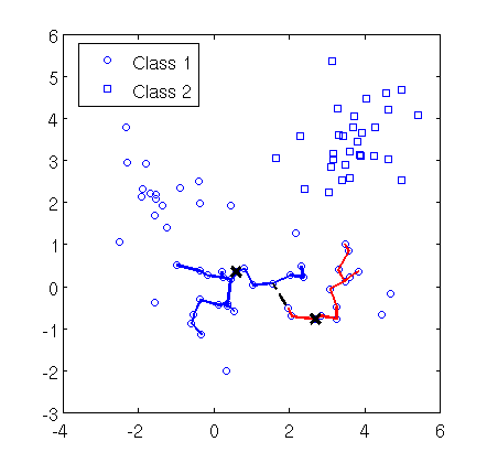

The MST based metric can be computationally intensive to compute as Prim’s algorithm must be run as many times as there are pairs of vertices. To counter this, Galluccio et al. (2013) proposed the EAC-DC algorithm which uses the information from only a subset of the dual rooted MSTs. This is done by calculating the dual rooted MSTs for a random pair of vertices. Three clusters are defined for each run: all vertices that are connected to one of the roots in the MSTs form two of the clusters (one for each root) while all points that are not connected to either of the MSTs are assigned to a third “rejection” cluster. A co-association measure for two vertices is then defined as the number of times those vertices are contained in the same non-rejection cluster divided by the total number of runs (dual rooted MSTs). This co-association measure forms a similarity measure to which spectral clustering is applied.
References
- Ahmed et al. (2011) Ahmed, O. W., R. Qahwaji, T. Colak, P. A. Higgins, P. T. Gallagher, and D. S. Bloomfield. Solar Flare Prediction Using Advanced Feature Extraction, Machine Learning, and Feature Selection. Solar Physics, 404, 2011. 10.1007/s11207-011-9896-1.
- Barnes et al. (2007) Barnes, G., K. D. Leka, E. A. Schumer, and D. J. Della-Rose. Probabilistic forecasting of solar flares from vector magnetogram data. Space Weather, 5, S09002, 2007. 10.1029/2007SW000317.
- Bazot et al. (2013) Bazot, C., N. Dobigeon, J.-Y. Tourneret, A. Zaas, G. Ginsburg, and A. O Hero III. Unsupervised Bayesian linear unmixing of gene expression microarrays. BMC Bioinformatics, 14(1), 99, 2013. 10.1186/1471-2105-14-99.
- Bhattacharyya (1946) Bhattacharyya, A. On a measure of divergence between two multinomial populations. Sankhyā: The Indian Journal of Statistics, 401–406, 1946.
- Bioucas-Dias et al. (2012) Bioucas-Dias, J. M., A. Plaza, N. Dobigeon, M. Parente, Q. Du, P. Gader, and J. Chanussot. Hyperspectral Unmixing Overview: Geometrical, Statistical, and Sparse Regression-Based Approaches. IEEE J. Sel. Topics Appl. Earth Observations Remote Sensing, 5(2), 354–379, 2012.
- Bobra and Couvidat (2015) Bobra, M. G., and S. Couvidat. Solar Flare Prediction Using SDO/HMI Vector Magnetic Field Data with a Machine-learning Algorithm. Astrophysical Journal, 798, 135, 2015. 10.1088/0004-637X/798/2/135.
- Bobra and Couvidat (2015) Bobra, M. G., and S. Couvidat. Solar Flare Prediction Using SDO/HMI Vector Magnetic Field Data with a Machine-Learning Algorithm. The Astrophysical Journal, 798(2), 135, 2015.
- Colak and Qahwaji (2008) Colak, T., and R. Qahwaji. Automated McIntosh-Based Classification of Sunspot Groups Using MDI Images. Solar Physics, 248, 277–296, 2008. 10.1007/s11207-007-9094-3.
- Colak and Qahwaji (2009) Colak, T., and R. Qahwaji. Automated Solar Activity Prediction: A hybrid computer platform using machine learning and solar imaging for automated prediction of solar flares. Space Weather, 7, S06001, 2009. 10.1029/2008SW000401.
- Comon and Jutten (2010) Comon, P., and C. Jutten. Handbook of Blind Source Separation: Independent Component Analysis and Blind Deconvolution. Academic Press, Oxford, 2010.
- Csiszar (1967) Csiszar, I. Information-type measures of difference of probability distributions and indirect observations. Studia Sci. Math. Hungar., 2, 299–318, 1967.
- DeForest (2004) DeForest, C. On re-sampling of solar images. Solar Physics, 219(1), 3–23, 2004.
- Ding et al. (2010) Ding, C., T. Li, and M. I. Jordan. Convex and semi-nonnegative matrix factorizations. Pattern Analysis and Machine Intelligence, IEEE Transactions on, 32(1), 45–55, 2010.
- Dudok de Wit et al. (2013) Dudok de Wit, T., S. Moussaoui, C. Guennou, F. Auchère, G. Cessateur, M. Kretzschmar, L. A. Vieira, and F. F. Goryaev. Coronal Temperature Maps from Solar EUV Images: A Blind Source Separation Approach. Solar Physics, 283, 31–47, 2013. 10.1007/s11207-012-0142-2.
- Edelman et al. (1998) Edelman, A., T. A. Arias, and S. T. Smith. The geometry of algorithms with orthogonality constraints. SIAM journal on Matrix Analysis and Applications, 20(2), 303–353, 1998.
- Falconer et al. (2008) Falconer, D. A., R. L. Moore, and G. A. Gary. Magnetogram Measures of Total Nonpotentiality for Prediction of Solar Coronal Mass Ejections from Active Regions of Any Degree of Magnetic Complexity. Astrophysical Journal, 689, 1433–1442, 2008. 10.1086/591045.
- Galluccio et al. (2013) Galluccio, L., O. Michel, P. Comon, M. Kliger, and A. O. Hero III. Clustering with a new distance measure based on a dual-rooted tree. Information Sciences, 251, 96–113, 2013.
- Georgoulis and Rust (2007) Georgoulis, M. K., and D. M. Rust. Quantitative Forecasting of Major Solar Flares. Astrophysical Journal, Letters, 661, L109–L112, 2007. 10.1086/518718.
- Guo et al. (2006) Guo, J., H. Zhang, O. V. Chumak, and Y. Liu. A Quantitative Study on Magnetic Configuration for Active Regions. Solar Physics, 237, 25–43, 2006. 10.1007/s11207-006-2081-2.
- Győri et al. (2010) Győri, L., T. Baranyi, and A. Ludmány. Photospheric data programs at the Debrecen Observatory. Proceedings of the International Astronomical Union, 6(S273), 403–407, 2010.
- Hale et al. (1919) Hale, G. E., F. Ellerman, S. B. Nicholson, and A. H. Joy. The Magnetic Polarity of Sun-Spots. Astrophysical Journal, 49, 153, 1919. 10.1086/142452.
- Hellinger (1909) Hellinger, E. Neue Begründung der Theorie quadratischer Formen von unendlichvielen Veränderlichen. Journal für die reine und angewandte Mathematik, 136, 210–271, 1909.
- Higgins et al. (2011) Higgins, P. A., P. T. Gallagher, R. McAteer, and D. S. Bloomfield. Solar magnetic feature detection and tracking for space weather monitoring. Advances in Space Research, 47(12), 2105–2117, 2011.
- Huang et al. (2010) Huang, X., D. Yu, Q. Hu, H. Wang, and Y. Cui. Short-Term Solar Flare Prediction Using Predictor Teams. Solar Physics, 263, 175–184, 2010. 10.1007/s11207-010-9542-3.
- Jolliffe (2002) Jolliffe, I. T. Principal Component Analysis, 2nd edition. Springer-Verlag New York, Inc., New York, 2002.
- Kruskal and Wish (1978) Kruskal, J. B., and M. Wish. Multidimensional Scaling, vol. 11. Sage, 1978.
- Kullback and Leibler (1951) Kullback, S., and R. A. Leibler. On information and sufficiency. The Annals of Mathematical Statistics, 79–86, 1951.
- Künzel (1960) Künzel, H. Die Flare-Häufigkeit in Fleckengruppen unterschiedlicher Klasse und magnetischer Struktur. Astronomische Nachrichten, 285, 271, 1960.
- Langville et al. (2006) Langville, A. N., C. D. Meyer, R. Albright, J. Cox, and D. Duling. Initializations for the nonnegative matrix factorization. In Proceedings of the Twelfth ACM SIGKDD International Conference on Knowledge Discovery and Data Mining, 23–26. Citeseer, 2006.
- Lee and Seung (2001) Lee, D. D., and H. S. Seung. Algorithms for non-negative matrix factorization. In Advances in Neural Information Processing Systems (NIPS), 556–562, 2001.
- Lee et al. (2012) Lee, K., Y.-J. Moon, J.-Y. Lee, K.-S. Lee, and H. Na. Solar Flare Occurrence Rate and Probability in Terms of the Sunspot Classification Supplemented with Sunspot Area and Its Changes. Solar Physics, 281, 639–650, 2012. 10.1007/s11207-012-0091-9.
- Leka and Barnes (2004) Leka, K. D., and G. Barnes. Photospheric Magnetic Field Properties of Flaring vs. Flare-Quiet Active Regions III: Discriminant Analysis of a Statistically Significant Database. In American Astronomical Society Meeting Abstracts #204, vol. 36 of Bulletin of the American Astronomical Society, 715, 2004.
- Lin (2007) Lin, C.-J. Projected gradient methods for nonnegative matrix factorization. Neural Computation, 19(10), 2756–2779, 2007.
- Mayfield and Lawrence (1985) Mayfield, E. B., and J. K. Lawrence. The correlation of solar flare production with magnetic energy in active regions. Solar Physics, 96, 293–305, 1985. 10.1007/BF00149685.
- Mittelman et al. (2012) Mittelman, R., N. Dobigeon, and A. Hero. Hyperspectral Image Unmixing Using a Multiresolution Sticky HDP. Signal Processing, IEEE Transactions on, 60(4), 1656–1671, 2012. 10.1109/TSP.2011.2180718.
- Moon and Hero III (2014a) Moon, K. R., and A. O. Hero III. Ensemble estimation of multivariate f-divergence. In Information Theory (ISIT), 2014 IEEE International Symposium on, 356–360. IEEE, 2014a.
- Moon and Hero III (2014b) Moon, K. R., and A. O. Hero III. Multivariate f-Divergence Estimation With Confidence. In Advances in Neural Information Processing Systems, vol. 27, 2420–2428, 2014b.
- Moon et al. (2015) Moon, K. R., J. J. Li, V. Delouille, R. De Visscher, F. Watson, and A. O. Hero, III. Image patch analysis of sunspots and active regions. I. Intrinsic dimension and correlation analysis. Journal of Space Weather and Space Climate, 2015.
- Moon et al. (2014) Moon, K. R., J. J. Li, V. Delouille, F. Watson, and A. O. Hero III. Image patch analysis and clustering of sunspots: A dimensionality reduction approach. In IEEE International Conference on Image Processing (ICIP), 1623–1627. IEEE, 2014.
- Moon and Stirling (2000) Moon, T. K., and W. C. Stirling. Mathematical Methods and Algorithms for Signal Processing. Prentice hall New York, 2000.
- Prim (1957) Prim, R. C. Shortest connection networks and some generalizations. Bell system technical journal, 36(6), 1389–1401, 1957.
- Ramírez and Sapiro (2012) Ramírez, I., and G. Sapiro. An MDL framework for sparse coding and dictionary learning. Signal Processing, IEEE Transactions on, 60(6), 2913–2927, 2012.
- Rand (1971) Rand, W. M. Objective criteria for the evaluation of clustering methods. Journal of the American Statistical Association, 66(336), 846–850, 1971.
- Rousseeuw (1987) Rousseeuw, P. J. Silhouettes: a graphical aid to the interpretation and validation of cluster analysis. Journal of Computational and Applied Mathematics, 20, 53–65, 1987.
- Sammis et al. (2000) Sammis, I., F. Tang, and H. Zirin. The Dependence of Large Flare Occurrence on the Magnetic Structure of Sunspots. Astrophysical Journal, 540, 583–587, 2000. 10.1086/309303.
- Scherrer et al. (1995) Scherrer, P. H., R. S. Bogart, R. I. Bush, J. T. Hoeksema, A. G. Kosovichev, et al. The Solar Oscillations Investigation - Michelson Doppler Imager. Solar Physics, 162, 129–188, 1995. 10.1007/BF00733429.
- Schrijver (2007) Schrijver, C. J. A Characteristic Magnetic Field Pattern Associated with All Major Solar Flares and Its Use in Flare Forecasting. Astrophysical Journal, Letters, 655, L117–L120, 2007. 10.1086/511857.
- Seichepine et al. (2014) Seichepine, N., S. Essid, C. Févotte, and O. Cappé. Soft nonnegative matrix co-factorization. Signal Processing, IEEE Transactions on, 62(22), 5940–5949, 2014.
- Sethian (1995) Sethian, J. A. A Fast Marching Level Set Method for Monotonically Advancing Fronts. In Proc. Nat. Acad. Sci, 1591–1595, 1995.
- Song et al. (2009) Song, H., C. Tan, J. Jing, H. Wang, V. Yurchyshyn, and V. Abramenko. Statistical Assessment of Photospheric Magnetic Features in Imminent Solar Flare Predictions. Solar Physics, 254, 101–125, 2009. 10.1007/s11207-008-9288-3.
- Stenning et al. (2013) Stenning, D. C., T. C. M. Lee, D. A. van Dyk, V. Kashyap, J. Sandell, and C. A. Young. Morphological feature extraction for statistical learning with applications to solar image data. Statistical Analysis and Data Mining, 6(4), 329–345, 2013. 10.1002/sam.11200.
- Stewart (1973) Stewart, G. W. Error and perturbation bounds for subspaces associated with certain eigenvalue problems. SIAM Review, 15(4), 727–764, 1973.
- Warwick (1966) Warwick, C. S. Sunspot Configurations and Proton Flares. Astrophysical Journal, 145, 215, 1966. 10.1086/148755.
- Watson et al. (2011) Watson, F. T., L. Fletcher, and S. Marshall. Evolution of sunspot properties during solar cycle 23. Astronomy & Astrophysics, 533, A14, 2011. 10.1051/0004-6361/201116655.
- Yaghoobi et al. (2009) Yaghoobi, M., T. Blumensath, and M. E. Davies. Dictionary learning for sparse approximations with the majorization method. Signal Processing, IEEE Transactions on, 57(6), 2178–2191, 2009.
- Yokoya et al. (2012) Yokoya, N., T. Yairi, and A. Iwasaki. Coupled nonnegative matrix factorization unmixing for hyperspectral and multispectral data fusion. Geoscience and Remote Sensing, IEEE Transactions on, 50(2), 528–537, 2012.
- Yu et al. (2010) Yu, D., X. Huang, H. Wang, Y. Cui, Q. Hu, and R. Zhou. Short-term Solar Flare Level Prediction Using a Bayesian Network Approach. Astrophysical Journal, 710, 869–877, 2010. 10.1088/0004-637X/710/1/869.