Algebraic and transcendental formulas for the smallest parts functionThanks: The first author was supported by a grant from the Simons Foundation (#208525 to Scott Ahlgren).

Scott Ahlgren Address: Department of Mathematics
University of Illinois
Urbana, IL 61801 Email address: sahlgren@illinois.edu and Nickolas Andersen Address: Department of Mathematics
University of Illinois
Urbana, IL 61801 Email address: nandrsn4@illinois.edu

Date: August 24, 2026

Abstract.

Building on work of Hardy and Ramanujan, Rademacher proved a well-known formula for the values of the ordinary partition function $p(n)$ . More recently, Bruinier and Ono obtained an algebraic formula for these values. Here we study the smallest parts function introduced by Andrews; $\spt(n)$ counts the number of smallest parts in the partitions of $n$ . The generating function for $\spt(n)$ forms a component of a natural mock modular form of weight $3/2$ whose shadow is the Dedekind eta function. Using automorphic methods (in particular the theta lift of Bruinier and Funke), we obtain an exact formula and an algebraic formula for its values. In contrast with the case of $p(n)$ , the convergence of our expression is non-trivial, and requires power savings estimates for weighted sums of Kloosterman sums for a multiplier in weight $1/2$ . These are proved with spectral methods (following an argument of Goldfeld and Sarnak).

1. Introduction

Let $p(n)$ denote the ordinary partition function. Hardy and Ramanujan [33] developed the circle method to prove the asymptotic formula

p(n)\sim\frac{e^{\pi\sqrt{\frac{2n}{3}}}}{4\sqrt{3}\,n}.

Building on their work, Rademacher [40, 41, 42] proved the famous formula

(1.1)

p(n)=\frac{2\pi}{(24n-1)^{3/4}}\sum_{c=1}^{\infty}\frac{A_{c}(n)}{c}I_{\frac{3}{2}}\left(\frac{\pi\sqrt{24n-1}}{6c}\right),

where $I_{\nu}$ is the $I$ -Bessel function, $A_{c}(n)$ is the Kloosterman sum

(1.2)

A_{c}(n):=\sum_{\begin{subarray}{c}d\bmod c\\ (d,c)=1\end{subarray}}e^{\pi is(d,c)}e\left(-\frac{dn}{c}\right),\quad e(x):=e^{2\pi ix}

and $s(d,c)$ is the Dedekind sum

(1.3)

s(d,c):=\sum_{r=1}^{c-1}\frac{r}{c}\left(\frac{dr}{c}-\left\lfloor\frac{dr}{c}\right\rfloor-\frac{1}{2}\right).

The existence of formula (1.1) is made possible by the fact that the generating function for $p(n)$ is a modular form of weight $-1/2$ , namely

q^{-\frac{1}{24}}\sum_{n\geq 0}p(n)q^{n}=\frac{1}{\eta(\tau)},\quad q:=\exp(2\pi i\tau),

where $\eta(\tau)$ denotes the Dedekind eta function.

There are a number of ways to prove (1.1). For example, Pribitkin [22] obtained a proof using a modified Poincaré series which represents $\eta^{-1}(\tau)$ . A similar technique can be used to obtain general formulas for the coefficients of modular forms of negative weight (see e.g. Hejhal [34, Appendix D] or Zuckerman [49]). The authors [2] recovered (1.1) from Poincaré series representing a weight $5/2$ harmonic Maass form whose shadow is $\eta^{-1}(\tau)$ . As pointed out by Bruinier and Ono [21], the exact formula can be recovered from the algebraic formula (1.7) stated below (this was partially carried out by Dewar and Murty [23]). The equivalence of (1.1) and (1.7) (in a more general setting) is made explicit by [7, Proposition 7].

The smallest parts function $\spt(n)$ , introduced by Andrews in [9], counts the number of smallest parts in the partitions of $n$ . Andrews proved that the generating function for $\spt(n)$ is given by

S(\tau):=\sum_{n\geq 1}\spt(n)q^{n}=\prod_{n\geq 1}\frac{1}{1-q^{n}}\left(\sum_{n\geq 1}\frac{nq^{n}}{1-q^{n}}+\sum_{n\neq 0}\frac{(-1)^{n}q^{n(3n+1)/2}}{(1-q^{n})^{2}}\right).

Work of Bringmann [13] shows that $S(\tau)$ is a component of a mock modular form of weight $3/2$ whose shadow is the Dedekind eta-function; using the circle method, she obtained an asymptotic expansion for $\spt(n)$ . In particular we have

\spt(n)\sim\frac{\sqrt{6n}}{\pi}\,p(n).

Many authors have investigated the coefficients of this mock modular form, which is a prototype for modular forms of this type (see, e.g., [3, 4, 10, 27, 29, 30, 31, 38]).

In analogy with (1.1), we prove the following formula for $\spt(n)$ .

Theorem 1.

For all $n\geq 1$ , we have

(1.4)

\spt(n)=\frac{\pi}{6}(24n-1)^{\frac{1}{4}}\sum_{c=1}^{\infty}\frac{A_{c}(n)}{c}\left(I_{1/2}-I_{3/2}\right)\left(\frac{\pi\sqrt{24n-1}}{6c}\right).

The convergence of Rademacher’s formula for $p(n)$ follows from elementary estimates on the size of the $I$ -Bessel function and the trivial bound $|A_{c}(n)|\leq c$ . By contrast, the convergence of the series for $\spt(n)$ is quite subtle, and requires non-trivial estimates for weighted sums of the Kloosterman sum (1.2). For this we utilize the spectral theory of half-integral weight Maass forms, discussed in more detail below.

We mention that Bringmann and Ono [14] established an exact formula for the coefficients of the weight $1/2$ mock theta function $f(q)$ ; this proved conjectures of Dragonette [25] and Andrews [8]. In this work they required estimates for Kloosterman sums of level $2$ , which were obtained by adapting a method of Hooley.

Formulas (1.1) and (1.4) express integers as infinite series involving values of transcendental functions. By contrast, Bruinier and Ono [21] (see also [15]) obtained a formula for $p(n)$ as a finite sum of algebraic numbers. Let $P(\tau)$ denote the $\Gamma_{0}(6)$ -invariant function

(1.5)

P(\tau):=-\frac{1}{2}\left(q\frac{d}{dq}+\frac{1}{2\pi y}\right)\frac{E_{2}(\tau)-2E_{2}(2\tau)-3E_{2}(3\tau)+6E_{2}(6\tau)}{(\eta(\tau)\eta(2\tau)\eta(3\tau)\eta(6\tau))^{2}}.

For $n\geq 1$ define

\mathcal{Q}_{1-24n}^{(1)}:=\left\{ax^{2}+bxy+cy^{2}:b^{2}-4ac=1-24n,\,6\mid a>0,\,\text{ and }b\equiv 1\bmod 12\right\}.

The group

(1.6)

\Gamma:=\Gamma_{0}(6)/\{\pm 1\}

acts on this set. For each $Q\in\mathcal{Q}_{1-24n}^{(1)}$ let $\tau_{Q}$ denote the root of $Q(\tau,1)$ in the upper-half plane $\mathbb{H}$ . Bruinier and Ono showed that

(1.7)

p(n)=\frac{1}{24n-1}\sum_{Q\in\Gamma\backslash\mathcal{Q}_{1-24n}^{(1)}}P(\tau_{Q}).

We obtain an analogue of (1.7) for $\spt(n)$ . Define the weakly holomorphic modular function

(1.8)

f(\tau):=\frac{1}{24}\frac{E_{4}(\tau)-4E_{4}(2\tau)-9E_{4}(3\tau)+36E_{4}(6\tau)}{(\eta(\tau)\eta(2\tau)\eta(3\tau)\eta(6\tau))^{2}}.

Then we have the following algebraic formula.

Theorem 2.

For all $n\geq 1$ , we have

(1.9)

\spt(n)=\frac{1}{12}\sum_{Q\in\Gamma\backslash\mathcal{Q}_{1-24n}^{(1)}}\left(f(\tau_{Q})-P(\tau_{Q})\right).

Bruinier and Ono showed that the values $P(\tau_{Q})$ are algebraic numbers with bounded denominators, and the classical theory of complex multiplication implies that the values $f(\tau_{Q})$ are algebraic as well (see, for instance, Section 6.1 of [48]).

The proof of Theorem 2 relies on the theta lift of Bruinier and Funke [20] which relates coefficients of harmonic Maass forms of weight $3/2$ to traces of CM values of modular functions. Generalizations of this lift are given in [5, 6, 21].

Example.

We illustrate the simplest case of Theorem 2. The class number of $\mathbb{Q}(\sqrt{-23})$ is $3$ , so $\Gamma\backslash\mathcal{Q}_{-23}^{(1)}$ consists of $3$ classes. These are represented by the forms

Q_{1}=6x^{2}+xy+y^{2},\quad Q_{2}=12x^{2}+13xy+4y^{2},\quad Q_{3}=18x^{2}+25xy+9y^{2},

whose roots are

\tau_{1}=\frac{-1+\sqrt{-23}}{12},\quad\tau_{2}=\frac{-13+\sqrt{-23}}{24},\quad\tau_{3}=\frac{-25+\sqrt{-23}}{36}.

Let $g=f-P$ . Since the values $\{g(\tau_{k})\}$ are conjugate algebraic numbers, we find that

(1.10)

\prod_{k=1,2,3}(x-g(\tau_{k}))=x^{3}-12x^{2}-\frac{1008}{23}x-\frac{1728}{23}

by approximating each $g(\tau_{k})$ using (1.5) and (1.8). This shows that $\spt(1)=1$ . Computing the roots of the polynomial in (1.10) gives the values

g(\tau_{1})=4\left(1+\frac{2}{23}\beta+\frac{22}{\beta}\right),\quad g(\tau_{2})=4\left(1+\frac{2}{23}\zeta_{3}\beta+\frac{22\zeta_{3}^{2}}{\beta}\right),\quad g(\tau_{3})=\overline{g(\tau_{2})},

where $\zeta_{3}:=e^{2\pi i/3}$ and

\beta:=\sqrt[3]{\frac{23}{2}\left(391+21\sqrt{69}\right)}.

We return to the problem of obtaining estimates for weighted sums of the $A_{c}(n)$ , which is of independent interest. Define

{\bf A}_{n}(x):=\sum_{c\leq x}\frac{A_{c}(n)}{c}.

Lehmer [37, Theorem 8] proved the sharp Weil-type bound

(1.11)

|A_{c}(n)|<2^{\omega_{o}(c)}\sqrt{c},

where $\omega_{o}(c)$ is the number of distinct odd primes dividing $c$ . Rademacher [43] later simplified Lehmer’s treatment of the sums $A_{c}(n)$ using Selberg’s formula [46]

A_{c}(n)=\sqrt{\frac{c}{3}}\sum_{\begin{subarray}{c}\ell\bmod{2c}\\ (3\ell^{2}+\ell)/2\equiv-n(c)\end{subarray}}(-1)^{\ell}\cos\left(\frac{6\ell+1}{6c}\pi\right).

From (1.11) we obtain

{\bf A}_{n}(x)\ll_{\epsilon}x^{\frac{1}{2}+\epsilon},

Since this is not sufficient to prove the convergence of the series in (1.4), we require a power savings estimate for ${\bf A}_{n}(x)$ . In Section 6 we adapt the method of Goldfeld and Sarnak [32] to relate ${\bf A}_{n}(x)$ to the spectrum of the weight $1/2$ hyperbolic Laplacian on ${\rm SL}_{2}(\mathbb{Z})\backslash\mathbb{H}$ . We prove a result which has the following corollary.

Theorem 3.

Suppose that $-n=\frac{k(3k\pm 1)}{2}$ is a pentagonal number. Then for any $\epsilon>0$ we have

\sum_{c\leq x}\frac{A_{c}(n)}{c}=(-1)^{k}\,\mathord{\raise 0.49991pt\hbox{$\displaystyle\genfrac{}{}{0.4pt}{}{12\sqrt{3}}{\pi^2}$}}\,x^{\frac{1}{2}}+O\left(x^{\frac{1}{6}+\epsilon}\right).

If $-n$ is not pentagonal then we have

\sum_{c\leq x}\frac{A_{c}(n)}{c}=O\left(x^{\frac{1}{6}+\epsilon}\right).

The implied constants depend on $n$ and $\epsilon$ .

This can be compared with Kuznetsov’s bound [36]

\sum_{c\leq x}\frac{k(m,n;c)}{c}\ll_{m,n}x^{\frac{1}{6}}(\log x)^{\frac{1}{3}}

where $k(m,n;c)$ is the ordinary Kloosterman sum defined in (4.3) below.

2. Preliminaries

We briefly introduce some of the objects which we will require.

2.1. Quadratic forms and Atkin-Lehner involutions

Let $M_{0}^{!}(\Gamma_{0}(N))$ denote the space of modular functions on $\Gamma_{0}(N)$ whose poles are supported at the cusps. We will mainly work with $N=6$ ; in this case, there are four cusps, one corresponding to each divisor of $6$ . To move among the cusps, the Atkin-Lehner involutions [11] are useful. For each divisor $d$ of $6$ , we define the Atkin-Lehner involution $W_{d}$ on $M_{0}^{!}(\Gamma_{0}(6))$ as the map $f\mapsto f\big|_{0}W_{d}$ , where

(2.1)

W_{1}=\left(\begin{matrix}1&0\\ 0&1\end{matrix}\right),\ W_{2}=\frac{1}{\sqrt{2}}\left(\begin{matrix}2&-1\\ 6&-2\end{matrix}\right),\ W_{3}=\frac{1}{\sqrt{3}}\left(\begin{matrix}3&1\\ 6&3\end{matrix}\right),\ W_{6}=\frac{1}{\sqrt{6}}\left(\begin{matrix}0&-1\\ 6&0\end{matrix}\right),

and $(f\big|_{0}\gamma)(\tau):=f(\gamma\tau)$ . The normalizing factors are chosen so that $W_{d}\in{\rm SL}_{2}(\mathbb{R})$ , which will be convenient later. If $d,d^{\prime}\mid 6$ , then

W_{d}W_{d^{\prime}}=W_{\frac{dd^{\prime}}{(d,d^{\prime})^{2}}}.

Suppose that $r\in\{1,5,7,11\}$ and that $D>0$ , and define

\mathcal{Q}_{-D}^{(r)}:=\left\{ax^{2}+bxy+cy^{2}:b^{2}-4ac=-D,\ 6\mid a>0,\text{ and }\ b\equiv r\bmod{12}\right\}.

Let $\Gamma_{0}^{*}(6)\subset{\rm SL}_{2}(\mathbb{R})$ denote the group generated by $\Gamma_{0}(6)$ and the Atkin-Lehner involutions $W_{d}$ for $d\mid 6$ . Matrices $g=\left(\begin{smallmatrix}\alpha&\beta\\ \gamma&\delta\end{smallmatrix}\right)\in\Gamma_{0}^{*}(6)$ act on binary quadratic forms on the left by

(2.2)

gQ(x,y):=Q(\delta x-\beta y,-\gamma x+\alpha y).

This action is compatible with the action $g\tau:=\frac{\alpha\tau+\beta}{\gamma\tau+\delta}$ on the root $\tau_{Q}\in\mathbb{H}$ of $Q(\tau,1)$ : for $g\in\Gamma_{0}^{*}(6)$ , we have

(2.3)

g\,\tau_{Q}=\tau_{gQ}.

Define

\mathcal{Q}_{-D}:=\bigcup_{r\in\{1,5,7,11\}}\mathcal{Q}_{-D}^{(r)}.

A computation involving (2.1) and (2.2) shows that

(2.4)

W_{d}:\mathcal{Q}_{-D}^{(r)}\longleftrightarrow\mathcal{Q}_{-D}^{(r^{\prime})}

is a bijection, where

(2.5)

r^{\prime}\equiv(2d\mu(d)-1)r\pmod{12}.

For each $r$ , we have

(2.6)

\mathcal{Q}_{-D}=\bigcup_{d|6}W_{d}\,\mathcal{Q}_{-D}^{(r)}.

2.2. Quadratic spaces of signature $(1,2)$

The proof of Theorem 2 uses a theta lift of Bruinier-Funke associated to an isotropic rational quadratic space of signature $(1,2)$ . To access the necessary results requires some background, which we develop briefly in the next two subsections. For further details, see [20, 18].

Let $V$ be an isotropic rational quadratic space of signature $(1,2)$ with non-degenerate symmetric bilinear form $(\cdot,\cdot)$ . Let the positive square-free integer $d$ denote the discriminant of the quadratic form $q$ given by $q(v)=\frac{1}{2}(v,v)$ . We may view $V$ as the subspace of pure quaternions with oriented basis

\left\{\left(\begin{matrix}0&1\\ -1&0\end{matrix}\right),\ \left(\begin{matrix}1&0\\ 0&-1\end{matrix}\right),\ \left(\begin{matrix}0&1\\ 1&0\end{matrix}\right)\right\}

in the quaternion algebra $M_{2}(\mathbb{Q})$ ; in other words we have

V=\left\{X=\left(\begin{matrix}x_{1}&x_{2}\\ x_{3}&-x_{1}\end{matrix}\right)\ :\ x_{i}\in\mathbb{Q}\right\}.

With this identification we have

q(X)=d\Det(X),\ \ \ (X,Y)=-d\Tr(XY).

We identify $G:=\operatorname*{Spin}(V)$ with ${\rm SL}_{2}(\mathbb{Q})$ and $\overline{G}\simeq\operatorname{PSL}_{2}(\mathbb{Q})$ with its image in $\operatorname{SO}(V)$ . The group $G$ acts on $V$ by conjugation; we write

g.X:=gXg^{-1}.

The group $G(\mathbb{R})$ acts transitively on the Grassmannian $\mathbb{D}$ of positive lines in $V$ :

\mathbb{D}:=\left\{z\subseteq V(\mathbb{R})\ :\ \dim z=1\ \ \text{and}\ \ q|_{z}>0\right\}.

Choosing the base point $z_{0}=\spn\left(\left(\begin{smallmatrix}0&1\\ -1&0\end{smallmatrix}\right)\right)\in\mathbb{D}$ , we find that $z_{0}$ is stabilized by $\operatorname{SO}_{2}(\mathbb{R})$ , so that

\mathbb{D}\simeq\operatorname{SO}_{2}(\mathbb{R})\backslash G(\mathbb{R})

is a Hermitian symmetric space.

An explicit isomorphism $\mathbb{H}\simeq\mathbb{D}$ can be described as follows. For $\tau=x+iy\in\mathbb{H}$ , let

g_{\tau}:=\frac{1}{\sqrt{y}}\left(\begin{matrix}x&-y\\ 1&0\end{matrix}\right)\in G(\mathbb{R}),

so that $g_{\tau}i=\tau$ . Then define

(2.7)

X(\tau):=g_{\tau}.\left(\begin{matrix}0&1\\ -1&0\end{matrix}\right)=\frac{1}{y}\left(\begin{matrix}-x&x^{2}+y^{2}\\ -1&x\end{matrix}\right),

and define an isomorphism $\mathbb{H}\rightarrow\mathbb{D}$ by $\tau\mapsto\spn\left(X(\tau)\right)$ . We have

(2.8)

X(g\tau)=g.X(\tau)

for all $g\in{\rm SL}_{2}(\mathbb{R})$ .

Let $L\subseteq V(\mathbb{Q})$ be the lattice

(2.9)

L:=\left\{\left(\begin{matrix}b&c/6\\ -a&-b\end{matrix}\right)\ :\ a,b,c\in\mathbb{Z}\right\}.

The dual lattice is

L^{\prime}=\left\{\left(\begin{matrix}b/12&c/6\\ -a&-b/12\end{matrix}\right)\ :\ a,b,c\in\mathbb{Z}\right\},

and we identify $L^{\prime}/L$ with $\mathbb{Z}/12\mathbb{Z}$ .

The group $\Gamma_{0}(6)\subseteq\operatorname*{Spin}(L)$ fixes $L$ . Let

\{\mathfrak{e}_{h}:h\in\mathbb{Z}/12\mathbb{Z}\}

denote the standard basis of the group ring $\mathbb{C}[L^{\prime}/L]$ . A computation shows that matrices $g=\left(\begin{smallmatrix}a&b\\ c&d\end{smallmatrix}\right)\in\Gamma_{0}^{*}(6)$ act on $\mathbb{C}[L^{\prime}/L]$ by

(2.10)

g.\mathfrak{e}_{h}=\mathfrak{e}_{(1+2bc)h}.

In particular, if $g\in\Gamma_{0}(6)$ , then $g$ acts trivially on $L^{\prime}/L$ .

Let

M:=\Gamma_{0}(6)\backslash\mathbb{D}

be the modular curve. If $X\in V(\mathbb{Q})$ has positive length, then we define

D_{X}:=\spn(X)\subseteq\mathbb{D}.

For each positive rational number $m$ and each $h\in L^{\prime}/L$ , define

L_{h,m}:=\left\{X\in L+h\ :\ q(X)=m\right\}.

Then $\Gamma_{0}(6)$ acts on $L_{h,m}$ with finitely many orbits.

The set $\operatorname{Iso}(V)$ of isotropic lines in $V(\mathbb{Q})$ is identified with the the cusps of $G(\mathbb{Q})$ via the map

(\alpha:\beta)\mapsto\spn\left(\left(\begin{matrix}-\alpha\beta&\alpha^{2}\\ -\beta^{2}&\alpha\beta\end{matrix}\right)\right).

The cusps of $M$ are the $\Gamma_{0}(6)$ classes of $\operatorname{Iso}(V)$ ; these are represented by the lines $\ell_{j}:=\spn(X_{j})$ , where

X_{0}:=\left(\begin{matrix}0&1\\ 0&0\end{matrix}\right),\ \ X_{1}:=\left(\begin{matrix}0&0\\ -1&0\end{matrix}\right),\ \ X_{2}:=\left(\begin{matrix}-2&1\\ -4&2\end{matrix}\right),\ \text{and}\ \ X_{3}:=\left(\begin{matrix}-3&1\\ -9&3\end{matrix}\right).

For each $\ell\in\operatorname{Iso}(V)$ choose $\sigma_{\ell}\in{\rm SL}_{2}(\mathbb{Z})$ with $\sigma_{\ell}\ell_{0}=\ell$ , and let $\alpha_{\ell}$ be the width of the cusp $\ell$ . For each $\ell$ , there is a positive rational number $\beta_{\ell}$ such that

\ell_{0}\cap\sigma_{\ell}^{-1}L=\left(\begin{matrix}0&\beta_{\ell}\mathbb{Z}\\ 0&0\end{matrix}\right),

and we define $\varepsilon_{\ell}:=\alpha_{\ell}/\beta_{\ell}$ .

Suppose that $q(X)<0$ and that $Q(X)\in-6(\mathbb{Q}^{\times})^{2}$ . Then (see [28, Lemma 3.6]) $X$ is orthogonal to two isotropic lines, $\spn(Y)$ and $\spn(\widetilde{Y})$ . We associate $\ell_{X}:=\spn(Y)$ to $X$ if $(X,Y,\widetilde{Y})$ is a positively oriented basis of $V$ . We then have $\ell_{-X}=\spn(\widetilde{Y})$ . For each $\ell$ , define

L_{h,-6m^{2},\ell}:=\left\{X\in L_{h,-6m^{2}}:\ell_{X}=\ell\right\}.

Then $\Gamma_{0}(6)$ acts on these sets, and equation (4.7) of [20] shows that

(2.11)

v_{\ell}(h,-6m^{2}):=\left|\Gamma_{0}(6)\backslash L_{h,-6m^{2},\ell}\right|=\begin{cases}2m\varepsilon_{\ell}&\text{ if }L_{h,-6m^{2},\ell}\neq\emptyset,\\ 0&\text{ otherwise.}\end{cases}

2.3. Harmonic Maass forms and the theta lift

Let $\Mp_{2}(\mathbb{R})$ denote the metaplectic two-fold cover of ${\rm SL}_{2}(\mathbb{R})$ . The elements of this group are pairs $(M,\phi(\tau))$ , where

M=\left(\begin{smallmatrix}a&b\\ c&d\end{smallmatrix}\right)\in{\rm SL}_{2}(\mathbb{R}),

and $\phi:\mathbb{H}\to\mathbb{C}$ is a holomorphic function satisfying $\phi(\tau)^{2}=(c\tau+d)$ .

Let $\Mp_{2}(\mathbb{Z})$ denote the inverse image of ${\rm SL}_{2}(\mathbb{Z})$ under the covering map; this group is generated by

T=\left(\left(\begin{matrix}1&1\\ 0&1\end{matrix}\right),1\right)\quad\text{ and }\quad S=\left(\left(\begin{matrix}0&-1\\ 1&0\end{matrix}\right),\sqrt{\tau}\right)

(here and throughout, we take the principal branch of $\sqrt{\cdot}$ ). We fix the lattice $L$ defined by (2.9). The Weil representation (see Chapter 1 of [17])

\rho_{L}:\Mp_{2}(\mathbb{Z})\to{\rm GL}\left(\mathbb{C}[L^{\prime}/L]\right)

is defined by

(2.12)		$\displaystyle\rho_{L}(T)\mathfrak{e}_{h}$	$\displaystyle=e\left(-\tfrac{h^{2}}{24}\right)\mathfrak{e}_{h},$
(2.12)		$\displaystyle\rho_{L}(S)\mathfrak{e}_{h}$	$\displaystyle=\frac{\sqrt{i}}{\sqrt{12}}\sum_{h^{\prime}\in L^{\prime}/L}e\left(\frac{hh^{\prime}}{12}\right)\mathfrak{e}_{h^{\prime}}.$

Denote by $H_{k,\rho_{L}}$ the space of weak harmonic Maass forms of weight $k$ for the representation $\rho_{L}$ ; these are functions $F:\mathbb{H}\to\mathbb{C}[L^{\prime}/L]$ which satisfy the following conditions:

(1)

For $(\gamma,\phi)\in\Mp_{2}(\mathbb{Z})$ ,

$f(\gamma\tau)=\phi(\tau)^{2k}\,\rho_{L}(\gamma,\phi)\,f(\tau).$

(2)

$\Delta_{k}f=0$ , where

\Delta_{k}:=-y^{2}\left(\frac{\partial^{2}}{\partial x^{2}}+\frac{\partial^{2}}{\partial y^{2}}\right)+iky\left(\frac{\partial}{\partial x}+i\frac{\partial}{\partial y}\right).

(3)

$f$ has at most linear exponential growth at $\infty$ .
(4)

$\xi_{k}f$ is holomorphic at $\infty$ , where

$\xi_{k}:=2iy^{k}\overline{\frac{\partial}{\partial\overline{\tau}}}.$

The theta lift of $f\in M_{0}^{!}(\Gamma_{0}(6))$ is given by

(2.13)

I(\tau,f):=\int_{M}f(z)\Theta(\tau,z)=\sum_{h\in L^{\prime}/L}I_{h}(\tau,f){\mathfrak{e}}_{h},

with

(2.14)

I_{h}(\tau,f):=\int_{M}f(z)\theta_{h}(\tau,z),

where $\theta_{h}(\tau,z)$ and $\Theta(\tau,z)$ are defined in §3.2 of [20].

We have

I(\tau,f)\in H_{\frac{3}{2},\rho_{L}}.

To see this, note that the transformation properties follow from those of the theta function (§3.2 of [20]). The other conditions follow from the explicit description of the Fourier expansion of $I(\tau,f)$ given in Theorem 4.5 of [20].

By (3.7) and (3.9) of [20] and (2.8) we have the relation

\theta_{h}(\tau,gz)=\theta_{g^{-1}h}(\tau,z)

for any $g\in\Gamma_{0}^{*}(6)$ . From this and (2.14) it follows that

(2.15)

I_{gh}(\tau,f)=I_{h}(\tau,f\big|_{0}g).

By Theorem 4.5 of [20] we have

(2.16)

I_{h}(\tau,f)=\sum_{m\geq 0}{\bf t}_{f}(h,m)q^{m}+\sum_{m>0}{\bf t}_{f}(h,-6m^{2})q^{-6m^{2}}+N(\tau).

A formula for the non-holomorphic part $N(\tau)$ is given in [20] but we do not include it here. Recall the definition (1.6). The terms of positive index $m$ in (2.16) are given by

(2.17)

{\bf t}_{f}(h,m)=\sum_{X\in\Gamma\backslash L_{h,m}}|\Gamma_{X}|^{-1}f(D_{X}),

where $\Gamma_{X}\subseteq\Gamma$ is the stabilizer of $X$ . Let

f\left(\sigma_{\ell}\tau\right)=\sum_{n\in\frac{1}{\alpha_{\ell}}\mathbb{Z}}a_{\ell}(n)q^{n}

denote the Fourier expansion of $f$ at the cusp $\ell$ , where $\alpha_{\ell}$ denotes the width of $\ell$ as in Section 2.2. By Proposition 4.7 of [20], the terms of negative index $-6m^{2}$ in (2.16) are given by

(2.18)

{\bf t}_{f}(h,-6m^{2})=-\!\!\!\!\!\sum_{\ell\in\Gamma\backslash\operatorname{Iso}(V)}\sum_{n\in\frac{2m}{\beta_{\ell}}\mathbb{N}}a_{\ell}(-n)\left(v_{\ell}(h,-6m^{2})e\left(\frac{r_{h,\ell}n}{2m}\right)+v_{\ell}(-h,-6m^{2})e\left(\frac{r_{-h,\ell}n}{2m}\right)\right),

where $r_{h,\ell}$ is defined by

\sigma_{\ell_{X}}^{-1}X=\left(\begin{matrix}m&r_{h,\ell}\\ 0&-m\end{matrix}\right)\ \text{ for any }X\in L_{h,-6m^{2},\ell}.

Note that ${\bf t}_{f}(h,-6m^{2})=0$ for $m$ sufficiently large.

3. Proof of the algebraic formula

The goal of this section is to prove Theorem 2. To prepare for the proof, recall the definition (1.8) of $f\in M_{0}^{!}(\Gamma_{0}(6))$ , and define $F(\tau)$ by

(3.1)		$\displaystyle F(\tau)$	$\displaystyle:=\sum_{n=1}^{\infty}\spt(n)q^{n-\frac{1}{24}}-\frac{1}{12}\cdot\frac{E_{2}(\tau)}{\eta(\tau)}+\frac{\sqrt{3i}}{2\pi}\int_{-\overline{\tau}}^{i\infty}\frac{\eta(w)}{\left(\tau+w\right)^{\frac{3}{2}}}dw$
(3.1)			$\displaystyle=\sum_{n=0}^{\infty}s(n)q^{n-\frac{1}{24}}+\frac{\sqrt{3i}}{2\pi}\int_{-\overline{\tau}}^{i\infty}\frac{\eta(w)}{\left(\tau+w\right)^{\frac{3}{2}}}dw,$

so that

(3.2)

s(n)=\spt(n)+\frac{1}{12}(24n-1)p(n).

Work of Bringmann [13] shows that $F(24\tau)$ is a harmonic Maass form on $\Gamma_{0}(576)$ of weight $3/2$ and character $\left(\frac{12}{\bullet}\right)$ , and that $F(24\tau)$ has eigenvalue $-1$ under the Fricke involution $W_{576}$ . Using these facts we find that

(3.3)

F(\tau+1)=e\left(-\tfrac{1}{24}\right)F(\tau),\qquad F(-1/\tau)=i^{\frac{1}{2}}\tau^{\frac{3}{2}}F(\tau).

Now set

(3.4)

\mathcal{F}(\tau):=\sum_{h\in L^{\prime}/L}\left(\tfrac{12}{h}\right)F(\tau){\mathfrak{e}}_{h}

(we use the identification of $L^{\prime}/L$ with $\mathbb{Z}/12\mathbb{Z}$ to define $\left(\tfrac{12}{h}\right)$ ). Using (3.3), (2.12), and the fact that

\sum_{h\in L^{\prime}/L}\left(\tfrac{12}{h}\right)e\left(\tfrac{hh^{\prime}}{12}\right)=\left(\tfrac{12}{h^{\prime}}\right)\sqrt{12},

we find that

\mathcal{F}(\tau)\in H_{\frac{3}{2},\rho_{L}}.

Proposition 4.

We have $I(\tau,f)=24\,\mathcal{F}(\tau)$ .

Proof.

For $d\mid 6$ we find that

(3.5)

f\big|_{0}W_{d}=\begin{cases}f&\text{ if }d=1,6,\\ -f&\text{ if }d=2,3.\end{cases}

We first claim that for $h\in L^{\prime}/L$ we have

(3.6)

I_{h}\left(\tau,f\right)=\left(\tfrac{12}{h}\right)I_{1}\left(\tau,f\right).

When $(h,12)=1$ the claim follows from (2.10), (2.14), (2.15) and (3.5). If $(h,12)\neq 1$ then by (2.10), $h$ is fixed by either $W_{2}$ or $W_{3}$ . In this case, (2.15) and (3.5) imply that $I_{h}(\tau,f)=0$ , and (3.6) follows.

Now let

\mathcal{G}(\tau)\in H_{\frac{3}{2},\rho_{L}}

denote the difference of the two forms in the statement of the lemma. By (3.4) and (3.6), there is a function $G$ such that

\mathcal{G}=\sum_{h\in L^{\prime}/L}\left(\tfrac{12}{h}\right)G\,\mathfrak{e}_{h}.

Arguing as above, we find that $G$ satisfies the transformation laws described by (3.3).

Using (2.18), we compute the principal part of $I_{1}(\tau,f)$ as follows. Since

\beta_{\ell_{0}}=\frac{1}{6},\quad\beta_{\ell_{1}}=1,\quad\beta_{\ell_{2}}=\frac{1}{2},\quad\text{ and }\quad\beta_{\ell_{3}}=\frac{1}{3},

we see that ${\bf t}_{f}(1,-6m^{2})=0$ for $m>\frac{1}{12}$ . A computation shows that

v_{\ell}(1,-\tfrac{1}{24})=\begin{cases}1&\text{ if }\ell=\ell_{0},\\ 0&\text{ otherwise,}\end{cases}\quad\text{ and }\quad v_{\ell}(-1,-\tfrac{1}{24})=\begin{cases}1&\text{ if }\ell=\ell_{1},\\ 0&\text{ otherwise.}\end{cases}

Furthermore, $r_{1,\ell_{0}}=r_{-1,\ell_{1}}=0$ , so ${\bf t}_{f}(1,-\frac{1}{24})=-2$ . Therefore the principal part of $I_{1}(\tau,f)$ is given by $-2q^{-1/24}$ , which agrees with the principal part of $24F(\tau)$ . It follows from (3.4) and (3.6) that $\mathcal{G}(\tau)$ has trivial principal part.

Let $g=\xi_{\frac{3}{2}}G$ . Then $g$ is holomorphic on $\mathbb{H}$ and at $\infty$ , and we have

g(\tau+1)=e\left(\tfrac{1}{24}\right)g(\tau)\quad\text{ and }\quad g(-1/\tau)=(-i)^{\frac{1}{2}}\tau^{\frac{1}{2}}\,g(\tau).

It follows that $g(\tau)$ is a constant multiple of $\eta(\tau)$ . Theorem 3.6 of [19] then implies that $\mathcal{G}(\tau)$ is a holomorphic modular form. It follows that $\mathcal{G}=0$ ; otherwise the product of $G$ with $\eta$ would be a non-zero modular form of weight $2$ for ${\rm SL}_{2}(\mathbb{Z})$ . ∎

Remark.

A more direct approach to the proof of Proposition 4 is to compute $N(\tau)$ using the formula in Theorem 4.5 of [20] and to match it directly to the non-holomorphic part of (3.1).

Proof of Theorem 2.

Suppose that $n\geq 1$ , and let $\widehat{n}:=n-\frac{1}{24}$ . By (2.16), (2.17), (3.1), and Proposition 4, we have

s(n)=\frac{1}{24}\sum_{X\in\Gamma\backslash L_{1,\widehat{n}}}|\Gamma_{X}|^{-1}f(D_{X}).

Note that for each $X$ , we have $D_{-X}=D_{X}$ , so we restrict our attention to the subset

L_{1,\widehat{n}}^{+}:=\left\{\left(\begin{matrix}b+\frac{1}{12}&\frac{c}{6}\\ -a&-b-\frac{1}{12}\end{matrix}\right):a,b,c\in\mathbb{Z},\ a>0,\text{ and }q(X)=\widehat{n}\right\}.

There is a natural bijection between $L_{1,\widehat{n}}^{+}$ and $\mathcal{Q}_{1-24n}^{(1)}$ given by

X=\left(\begin{matrix}b+\frac{1}{12}&\frac{c}{6}\\ -a&-b-\frac{1}{12}\end{matrix}\right)\longleftrightarrow Q_{X}:=[6a,12b+1,c].

It is easy to check that the action of $\Gamma$ on $L_{1,\widehat{n}}$ translates under this bijection to the usual action of $\Gamma$ on $\mathcal{Q}_{1-24n}^{(1)}$ . Since the stabilizer of $Q$ is trivial for every $Q\in\mathcal{Q}_{1-24n}^{(1)}$ , we have $|\Gamma_{X}|=1$ for all $X\in\Gamma\backslash L_{1,\widehat{n}}^{+}$ . A computation involving (2.7) shows that $D_{X}\mapsto\tau_{Q_{X}}$ under the isomorphism $\mathbb{D}\cong\mathbb{H}$ . Thus we have

s(n)=\frac{1}{12}\sum_{Q\in\Gamma\backslash\mathcal{Q}_{1-24n}^{(1)}}f(\tau_{Q}).

The theorem follows from (1.7) and (3.2). ∎

4. Poincaré series and the function $f(\tau)$

In this section we construct the modular function $f(\tau)$ in terms of weak Maass-Poincaré series. To this end, we construct an auxiliary function $f(\tau,s)$ , defined for $\re(s)>1$ and compute its Fourier expansion to obtain an analytic continuation of $f(\tau,s)$ to $\re(s)>\frac{3}{4}$ . We then show that $f(\tau,1)=f(\tau)$ .

Recall (1.6) and write

\tau=x+iy,\qquad s=\sigma+it.

Letting $\Gamma_{\infty}=\{\left(\begin{smallmatrix}1&*\\ 0&1\end{smallmatrix}\right)\}$ denote the stabilizer of $\infty$ , we define

F(\tau,s):=\sum_{\gamma\in\Gamma_{\infty}\backslash\Gamma}\phi_{s}(\im\gamma\tau)e(-\re\gamma\tau),

where

(4.1)

\phi_{s}(y):=2\pi\sqrt{y}\,I_{s-\frac{1}{2}}(2\pi y).

Since $\phi_{s}(y)\ll y^{\sigma}$ as $y\to 0$ , we have

F(\tau,s)\ll y^{\sigma}\sum_{\left(\begin{smallmatrix}*&*\\ c&d\end{smallmatrix}\right)\in\Gamma_{\infty}\backslash\Gamma}|c\tau+d|^{-2\sigma},

so $F(\tau,s)$ converges normally for $\sigma>1$ . A computation involving (13.14.1) of [24] shows that

(4.2)

\Delta_{0}F(\tau,s)=s(1-s)F(\tau,s).

Let $\mu$ denote the Möbius function, and define

f(\tau,s):=\sum_{r\mid 6}\mu(r)F(W_{r}\tau,s).

The following proposition gives the Fourier expansion of $f(\tau,s)$ in terms of the ordinary Kloosterman sum

(4.3)

k(m,n;c):=\sum_{\begin{subarray}{c}d\bmod c\\ (c,d)=1\end{subarray}}e\left(\frac{m\overline{d}+nd}{c}\right)

and the $I$ , $J$ , and $K$ -Bessel functions (here $\overline{d}$ is the multiplicative inverse of $d$ modulo $c$ ).

Proposition 5.

For $\sigma>1$ we have

f(\tau,s)=2\pi\sqrt{y}\,I_{s-\frac{1}{2}}(2\pi y)e(-x)+a_{s}(0)y^{1-s}+2\sqrt{y}\,\sum_{n\neq 0}a_{s}(n)K_{s-\frac{1}{2}}(2\pi|n|y)e(nx),

where

	$\displaystyle a_{s}(0)$	$\displaystyle=\frac{2\pi^{s+1}}{(s-\frac{1}{2})\Gamma(s)}\sum_{r\mid 6}\mu(r)\sum_{\begin{subarray}{c}0<c\equiv 0(6/r)\\ (c,r)=1\end{subarray}}\frac{k(-\overline{r},0;c)}{(c\sqrt{r})^{2s}},$
	$\displaystyle a_{s}(n)$	$\displaystyle=2\pi\sum_{r\mid 6}\mu(r)\sum_{\begin{subarray}{c}0<c\equiv 0(6/r)\\ (c,r)=1\end{subarray}}\frac{k(-\overline{r},n;c)}{c\sqrt{r}}\times\begin{cases}I_{2s-1}\left(\frac{4\pi\sqrt{n}}{c\sqrt{r}}\right)&\text{ if }n>0,\\ J_{2s-1}\left(\frac{4\pi\sqrt{\|n\|}}{c\sqrt{r}}\right)&\text{ if }n<0.\end{cases}$

Proof.

The function $f(\tau,s)-\phi_{s}(y)e(-x)$ has at most polynomial growth as $y\to\infty$ . For $r\mid 6$ , $r\neq 1$ , a complete set of representatives for $\Gamma_{\infty}\backslash\Gamma W_{r}$ is given by

\left\{\left(\begin{matrix}ra&*\\ rc&rd\end{matrix}\right):\ c>0,\ \gcd(c,rd)=1,\ (6/r)\mid c,\ a\in\{1,\dots,c-1\},\ a\equiv\overline{rd}\pmod{c}\right\}.

So we have the Fourier expansion

f(\tau,s)=\phi_{s}(y)e(-x)+\sum_{n\in\mathbb{Z}}\sum_{r\mid 6}\mu(r)A_{r}(n,y,s)e(nx),

where

\displaystyle A_{r}(n,y,s)

\displaystyle=\sum_{\begin{subarray}{c}\gamma\in\Gamma_{\infty}\backslash\Gamma W_{r}\\ c(\gamma)>0\end{subarray}}\int_{0}^{1}\phi_{s}(\im\gamma\tau)e(-\re\gamma\tau)e(-nx)\,dx.

For $\gamma=\left(\begin{smallmatrix}ra&b\\ rc&rd\end{smallmatrix}\right)\in\Gamma_{\infty}\backslash\Gamma W_{r}$ with $c(\gamma)>0$ we write

\gamma\tau=\frac{ra\,\tau+b}{rc\,\tau+rd}=\frac{a}{c}-\frac{1}{rc^{2}(\tau+d/c)}

and make the change of variable $x\to x-d/c$ to obtain

\displaystyle A_{r}(n,y,s)

\displaystyle=\sum_{\begin{subarray}{c}0<c\equiv 0(6/r)\\ (c,rd)=1\end{subarray}}e\left(\frac{-a+nd}{c}\right)\int_{d/c}^{1+d/c}\phi_{s}\left(\frac{y}{rc^{2}|\tau|^{2}}\right)e\left(\frac{x}{rc^{2}|\tau|^{2}}-nx\right)\,dx.

Since $a\equiv\overline{rd}\pmod{c}$ we have

\sum_{\begin{subarray}{c}d\bmod c\\ (d,c)=1\end{subarray}}e\left(\frac{-a+nd}{c}\right)=k(-\overline{r},n;c),

so that

\displaystyle A_{r}(n,y,s)

\displaystyle=2\pi\sum_{\begin{subarray}{c}0<c\equiv 0(6/r)\\ (r,c)=1\end{subarray}}\frac{k(-\overline{r},n;c)}{c\sqrt{r}}y^{\frac{1}{2}}\int_{-\infty}^{\infty}|\tau|^{-1}\,I_{s-\frac{1}{2}}\left(\frac{2\pi y}{rc^{2}|\tau|^{2}}\right)e\left(\frac{x}{rc^{2}|\tau|^{2}}-nx\right)\,dx.

Let $I$ denote the integral above. We make the substitution $x=yu$ and set $A=\frac{1}{rc^{2}y}$ and $B=-ny$ , so that

I=\int_{-\infty}^{\infty}(u^{2}+1)^{-\frac{1}{2}}I_{s-\frac{1}{2}}\left(\frac{2\pi A}{u^{2}+1}\right)e\left(\frac{Au}{u^{2}+1}+Bu\right)\,du.

Using Lemma 5.5 on page 357 and (xiv) and (xv) on page 345 of [34], and the fact that

2^{1-2s}\sqrt{\pi}\,\frac{\Gamma(2s)}{\Gamma(s+\frac{1}{2})\Gamma(s)}=1,

we find that

I=\begin{cases}2K_{s-\frac{1}{2}}(2\pi B)J_{2s-1}\left(4\pi\sqrt{AB}\right)&\text{ if }B>0,\\ \frac{\pi^{s}A^{s-\frac{1}{2}}}{(s-\frac{1}{2})\Gamma(s)}&\text{ if }B=0,\\ 2K_{s-\frac{1}{2}}(2\pi|B|)I_{2s-1}\left(4\pi\sqrt{A|B|}\right)&\text{ if }B<0.\end{cases}

The proposition follows. ∎

The function $f(\tau,s)$ has an analytic continuation to $\sigma>\frac{3}{4}$ , as we now show. Suppose that $\frac{3}{4}<\sigma_{0}<\frac{3}{2}$ , and fix $\epsilon_{0}$ with $0<\epsilon_{0}<2\sigma_{0}-\frac{3}{2}$ . We will show that the Fourier expansion in Proposition 5 converges absolutely and uniformly for $s$ in the region $R$ defined by $\sigma_{0}\leq\sigma\leq\frac{3}{2}$ , $|t|\leq T$ (the estimates below are for $s\in R$ ). Using the Weil bound [45] for Kloosterman sums we have

k(a,b;c)\ll\gcd(a,b,c)^{\frac{1}{2}}c^{\frac{1}{2}+\epsilon_{0}},

from which

a_{s}(0)\ll\sum_{c>0}c^{-2\sigma_{0}+\frac{1}{2}+\epsilon_{0}}\ll 1.

By (10.40.2) of [24] we have

(4.4)

\sqrt{y}\,K_{s-\frac{1}{2}}(2\pi|n|y)\ll|n|^{-\frac{1}{2}}e^{-2\pi|n|y}\quad\text{as $n\to\infty$}.

From (10.40.1) and (10.30.1) of [24] we have

	$\displaystyle I_{2s-1}(x)\ll\frac{e^{x}}{\sqrt{x}}\quad\text{as }x\to\infty,$
	$\displaystyle I_{2s-1}(x)\ll x^{2s-1}\quad\text{as }x\to 0.$

Suppose that $n>0$ . Taking absolute values in the series defining $a_{s}(n)$ , we find that

(4.5)

a_{s}(n)\ll n^{-\frac{1}{4}}\sum_{c<\sqrt{n}}c^{\epsilon_{0}}\,e^{\frac{4\pi\sqrt{n}}{c}}+n\sum_{c\geq\sqrt{n}}c^{-2\sigma_{0}+\frac{1}{2}+\epsilon_{0}}\ll e^{4\pi\sqrt{n}}n^{\frac{1}{4}+\epsilon_{0}}+n\ll e^{6\pi\sqrt{n}}.

From (10.7.8) and (10.7.3) of [24] we have

	$\displaystyle J_{2s-1}(x)\ll\frac{1}{\sqrt{x}}\quad\text{as }x\to\infty,$
	$\displaystyle J_{2s-1}(x)\ll x^{2s-1}\quad\text{as }x\to 0.$

Arguing as above we find that for $n<0$ we have $a_{s}(n)\ll n$ . With (4.5) and (4.4), this shows that the Fourier expansion converges absolutely and uniformly for $s\in R$ . This provides the analytic continuation of $f(\tau,s)$ to $\sigma>\frac{3}{4}$ .

Since

2\sqrt{y}\,K_{\frac{1}{2}}(2\pi|n|y)=|n|^{-\frac{1}{2}}e^{-2\pi|n|y}\quad\text{ and }\quad 2\pi\sqrt{y}\,I_{\frac{1}{2}}(2\pi y)=2\sinh(2\pi y),

the Fourier expansion of $f(\tau,1)$ is

(4.6)

f(\tau,1)=e(-\tau)+a_{1}(0)+\sum_{n>0}\frac{a_{1}(n)}{\sqrt{n}}e(n\tau)-e(-\overline{\tau})+\sum_{n<0}\frac{a_{1}(n)}{\sqrt{|n|}}e(n\overline{\tau}).

Using (4.2) and (4.6) we find that $\xi_{0}f(\tau,1)$ is a cusp form of weight $2$ on $\Gamma_{0}(6)$ , so it equals $0$ . Therefore $f(\tau,1)$ is holomorphic on $\mathbb{H}$ . Since the principal parts of $f(\tau,1)$ and $f(\tau)$ are equal, we conclude that

(4.7)

f(\tau,1)=f(\tau),

as desired.

5. Proof of Theorem 1

By Theorem 2 and equations (4.7), (3.2), and (2.3) we have

	$\displaystyle s(n)$	$\displaystyle=\frac{1}{12}\sum_{Q\in\Gamma\backslash\mathcal{Q}_{1-24n}^{(1)}}f(\tau_{Q})$
		$\displaystyle=\lim_{s\to 1^{+}}\frac{1}{12}\sum_{Q\in\Gamma\backslash\mathcal{Q}_{1-24n}^{(1)}}\sum_{d\mid 6}\sum_{\gamma\in\Gamma_{\infty}\backslash\Gamma}\mu(d)\phi_{s}(\im\tau_{\gamma W_{d}Q})e(-\re\tau_{\gamma W_{d}Q}).$

By (2.4) and (2.6) the map $\left(\gamma,d,Q\right)\mapsto\gamma W_{d}\,Q$ is a bijection

(5.1)

\Gamma_{\infty}\backslash\Gamma\times\{1,2,3,6\}\times\Gamma\backslash\mathcal{Q}^{(1)}_{1-24n}\longleftrightarrow\Gamma_{\infty}\backslash\mathcal{Q}_{1-24n}.

If $Q\in\mathcal{Q}_{1-24n}^{(1)}$ and $Q^{\prime}=W_{d}Q=[a,b,*]$ then $\mu(d)=\left(\frac{12}{b}\right)$ by (2.4) and (2.5). Thus we have

\displaystyle s(n)=\lim_{s\to 1^{+}}\frac{1}{12}\sum_{\begin{subarray}{c}Q\in\Gamma_{\infty}\backslash\mathcal{Q}_{1-24n}\\ Q=[a,b,*]\end{subarray}}\left(\frac{12}{b}\right)\phi_{s}\left(\frac{\sqrt{24n-1}}{2a}\right)e\left(\frac{b}{2a}\right).

Since $\left(\begin{smallmatrix}1&k\\ 0&1\end{smallmatrix}\right)[a,b,*]=[a,b-2ka,*]$ , there is a bijection

\Gamma_{\infty}\backslash\mathcal{Q}_{1-24n}\longleftrightarrow\left\{(a,b):a>0,\ \ 6\mid a,\ \ 0\leq b<2a,\ \ b^{2}\equiv 1-24n\pmod{4a}\right\},

which, together with (4.1), gives

\displaystyle s(n)

\displaystyle=\lim_{s\to 1^{+}}\frac{\pi}{6\sqrt{2}}(24n-1)^{\frac{1}{4}}\sum_{6\mid a>0}a^{-\frac{1}{2}}I_{s-\frac{1}{2}}\left(\frac{\pi\sqrt{24n-1}}{a}\right)\sum_{\begin{subarray}{c}b\bmod{2a}\\ b^{2}\equiv 1-24n(4a)\end{subarray}}\left(\frac{12}{b}\right)e\left(\frac{b}{2a}\right).

Writing $a=6c$ , we see that the inner sum is equal to

\frac{1}{2}\sum_{\begin{subarray}{c}b\bmod 24c\\ b^{2}\equiv 1-24n(24c)\end{subarray}}\left(\frac{12}{b}\right)e\left(\frac{-b}{12c}\right).

By Proposition 6 of [7] (see also [46]), this equals

\frac{2\sqrt{3}}{\sqrt{c}}A_{c}(n).

We conclude that

(5.2)

s(n)=\lim_{s\to 1^{+}}\frac{\pi}{6}(24n-1)^{\frac{1}{4}}\sum_{c=1}^{\infty}\frac{A_{c}(n)}{c}I_{s-\frac{1}{2}}\left(\frac{\pi\sqrt{24n-1}}{6c}\right).

To finish the proof of Theorem 1 we need to interchange the limit and the sum in (5.2). To justify this, we apply partial summation and Theorem 3.

Set $a:=\frac{\pi\sqrt{24n-1}}{6}$ , suppose that $s\in[1,2]$ , and define

(5.3)

{\bf A}_{n}(x):=\sum_{c\leq x}\frac{A_{c}(n)}{c}.

By Theorem 3 we have ${\bf A}_{n}(x)\ll_{\epsilon,n}x^{\frac{1}{6}+\epsilon}$ for any $\epsilon>0$ . Partial summation, together with (5.5) and Lemma 6 below, gives

	$\displaystyle\sum_{c>N}\frac{A_{c}(n)}{c}I_{s-\frac{1}{2}}\left(\frac{a}{c}\right)$	$\displaystyle=\lim_{x\to\infty}{\bf A}_{n}(x)I_{s-\frac{1}{2}}\left(\frac{a}{x}\right)-{\bf A}_{n}(N)I_{s-\frac{1}{2}}\left(\frac{a}{N}\right)-\int_{N}^{\infty}{\bf A}_{n}(t)\left(I_{s-\frac{1}{2}}(a/t)\right)^{\prime}\,dt$
		$\displaystyle\ll_{a}N^{\frac{2}{3}-s+\epsilon}+\int_{N}^{\infty}t^{-\frac{1}{3}-s+\epsilon}\,dt\ll_{a}N^{-\frac{1}{3}+\epsilon}.$

It follows that the series (5.2) converges uniformly for $s\in[1,2]$ . Interchanging the limit and the sum gives Theorem 1. It remains to prove the following straightforward lemma.

Lemma 6.

Suppose that $a>0$ is fixed and that $\frac{1}{2}\leq\nu\leq\frac{3}{2}$ . Then

\left|\left(I_{\nu}(a/x)\right)^{\prime}\right|\ll_{a}{x^{-\nu-1}}\ \ \ \text{as $x\to\infty$}.

Proof.

By (10.29.1) of [24] we find that

I_{\nu}^{\prime}(x)=\tfrac{1}{2}\left(I_{\nu-1}(x)+I_{\nu+1}(x)\right).

For fixed $x$ , the function $I_{\nu}(x)$ is decreasing as a function of $\nu$ . Therefore

(5.4)

\left|\left(I_{\nu}(a/x)\right)^{\prime}\right|=\frac{a}{2x^{2}}\left(I_{\nu-1}(a/x)+I_{\nu+1}(a/x)\right)\leq\frac{a}{x^{2}}I_{\nu-1}(a/x).

From (10.30.1) of [24] we have

(5.5)

I_{\nu}(a/x)\ll_{a}x^{-\nu}\ \ \text{as $x\to\infty$ \ \ for \ \ $\nu\in[1/2,3/2]$}.

The lemma follows from (5.4) and (5.5). ∎

6. Sums of Kloosterman sums

In this section we will consider sums of Kloosterman sums $S(m,n,c,\chi)$ associated to a multiplier in weight $k$ , which were studied when $m,n>0$ by Goldfeld and Sarnak [32]. Work of Folsom-Ono [26] and Pribitkin [39] applies to the case of general $m$ and $n$ . For completeness we record a general asympotic formula here, referring the reader to [32] for details.

Let $\Gamma$ be a finite-index subgroup of ${\rm SL}_{2}(\mathbb{Z})$ which contains $-I$ . Suppose that $k\in\mathbb{R}$ and that $\chi$ is a multiplier on $\Gamma$ for the weight $k$ . Suppose that $q$ is the smallest positive integer for which $\left(\begin{smallmatrix}1&q\\ 0&1\end{smallmatrix}\right)\in\Gamma$ and define $\alpha\in[0,1)$ by

\chi\left(\!\left(\begin{matrix}1&q\\ 0&1\end{matrix}\right)\!\right)=e(-\alpha).

For simplicity, we write

\widetilde{n}:=\frac{n-\alpha}{q}.

For $c>0$ , the generalized Kloosterman sum is given by

S(m,n,c,\chi):=\sum_{\begin{subarray}{c}0\leq\,a,d\,<qc\\ \gamma=\left(\begin{smallmatrix}a&b\\ c&d\end{smallmatrix}\right)\in\Gamma\end{subarray}}\overline{\chi(\gamma)}\,e\left(\frac{\widetilde{m}a+\widetilde{n}d}{c}\right),

and Selberg’s Kloosterman zeta function is defined as

Z_{m,n}(s,\chi):=\sum_{c>0}\frac{S(m,n,c,\chi)}{c^{2s}}.

The space $L^{2}\left(\Gamma\backslash\mathbb{H},\chi,k\right)$ consists of functions $f:\mathbb{H}\to\mathbb{C}$ such that

f\left(\gamma\tau\right)=\chi(\gamma)\left(\frac{c\tau+d}{|c\tau+d|}\right)^{k}f(\tau)\quad\text{ for all }\gamma\in\Gamma

and $\|f\|<\infty$ , where

\|f\|^{2}:=\iint_{\Gamma\backslash\mathbb{H}}|f(\tau)|^{2}\,\frac{dxdy}{y^{2}}.

The operator

\widetilde{\Delta}_{k}:=y^{2}\left(\frac{\partial^{2}}{\partial x^{2}}+\frac{\partial^{2}}{\partial y^{2}}\right)-iky\frac{\partial}{\partial x}

(which is not the operator $\Delta_{k}$ in §2.3) has a self-adjoint extension to $L^{2}\left(\Gamma\backslash\mathbb{H},\chi,k\right)$ with real spectrum. The asymptotic formula of [32] depends on the discrete spectrum, which we denote by

\lambda_{0}\leq\lambda_{1}\leq\lambda_{2}\leq\dots.

For each $j$ with $\lambda_{j}<\frac{1}{4}$ let $u_{j}$ be the normalized Maass cusp form corresponding to $\lambda_{j}$ and define $s_{j}\in\left(\frac{1}{2},1\right)$ by

\lambda_{j}=s_{j}(1-s_{j}).

We have the expansion

(6.1)

u_{j}(\tau)=\sum_{m=-\infty}^{\infty}\widehat{u}_{j}(m,y)e(\widetilde{m}x),

where

(6.2)

\widehat{u}_{j}(m,y)=\begin{cases}\rho_{j}(m)W_{\frac{k}{2}\sgn(\widetilde{m}),s_{j}-\frac{1}{2}}(4\pi|\widetilde{m}|y)e(\widetilde{m}x)&\text{ if }\widetilde{m}\neq 0,\\ \rho_{j}(0)y^{s_{j}}+\rho^{\prime}_{j}(0)y^{1-s_{j}}&\text{ if }\widetilde{m}=0.\end{cases}

Define

\beta:=\limsup_{c\to\infty}\frac{\log|S(m,n,c,\chi)|}{\log c}.

With this notation we have the following

Proposition 7.

Suppose that $m>0$ and that $n\in\mathbb{Z}$ . For any $\epsilon>0$ we have

\sum_{c\leq x}\frac{S(m,n,c,\chi)}{c}=\sum_{\frac{1}{2}<s_{j}<1}\tau_{j}(m,n)\frac{x^{2s_{j}-1}}{2s_{j}-1}+O\left(x^{\frac{\beta}{3}+\epsilon}\right),

where the sum runs over those $j$ with $\lambda_{j}<\frac{1}{4}$ as above and

(6.3)

\tau_{j}(m,n)=2q^{2}i^{k}\,\overline{\rho_{j}(m)}\rho_{j}(n)\pi^{1-2s_{j}}(4\widetilde{m}|\widetilde{n}|)^{1-s_{j}}\frac{\Gamma\left(s_{j}+\sgn(\widetilde{n})\frac{k}{2}\right)\Gamma\left(2s_{j}-1\right)}{\Gamma\left(s_{j}-\frac{k}{2}\right)}.

The implied constant depends on $k$ , $\chi$ , $m$ , $n$ , $\epsilon$ , and $\Gamma$ .

When $n>0$ this is Theorem 2 of [32], but the constants in (3.2) of [32] differ from those in (6.3). Figure 1 in Section 7 gives an example which supports the accuracy of (6.3). The existence of such a formula is implicit in [26].

For the case when $n\leq 0$ we argue as in Lemma 2 of [32], relating $Z_{m,n}(s,\chi)$ to the inner product of two Poincaré series. We compute

\langle P_{m}\left(\tau,s,\chi,k\right),\overline{P_{1-n}\left(\tau,s+2,\overline{\chi},-k\right)}\rangle=\frac{(-i)^{k}}{4^{s+1}\pi\widetilde{n}^{2}}\cdot\frac{\Gamma\left(2s+1\right)}{\Gamma\left(s-\frac{k}{2}\right)\Gamma\left(s+\frac{k}{2}+2\right)}Z_{m,n}(s,\chi)+R(s),

where $R(s)$ is holomorphic in $\sigma>\frac{1}{2}$ and is $O\left(\frac{1}{\sigma-\frac{1}{2}}\right)$ in this region. Arguing as in Section 2 of [32] we find that for $m>0$ and for all $n$ we have

\operatorname*{Res}_{s=s_{j}}Z_{m,n}(s,\chi)=q^{2}i^{k}\overline{\rho_{j}(m)}\rho_{j}(n)\pi^{1-2s_{j}}(4\widetilde{m}|\widetilde{n}|)^{1-s_{j}}\frac{\Gamma\left(s_{j}+\sgn(\widetilde{n})\frac{k}{2}\right)\Gamma\left(2s_{j}-1\right)}{\Gamma\left(s_{j}-\frac{k}{2}\right)}.

The proposition follows by the method of Section 3 of [32].

7. Sums of Kloosterman sums for the $\eta$ -multiplier

We specialize the results of Section 6 to $k=\frac{1}{2}$ , $\Gamma={\rm SL}_{2}(\mathbb{Z})$ , and $\chi$ the multiplier system attached to the $\eta$ -function. For matrices in ${\rm SL}_{2}(\mathbb{Z})$ with $c>0$ we have (see, for example, §2.8 of [35])

(7.1)

\chi\left(\!\left(\begin{matrix}a&b\\ c&d\end{matrix}\right)\!\right)=\sqrt{-i}\,e\left(\frac{a+d}{24c}\right)e^{-\pi is(d,c)},

where $s(d,c)$ is the Dedekind sum defined in (1.3). In this case we have $q=1$ and $\alpha=\frac{23}{24}$ . Recall that the pentagonal numbers are those numbers of the form $\frac{k(3k\pm 1)}{2}$ for $k\in\mathbb{Z}$ . We have the following (c.f. [44, Theorem 4.5]).

Theorem 8.

Suppose that $m>0$ and that $n\in\mathbb{Z}$ . If $m-1=\frac{k_{1}(3k_{1}\pm 1)}{2}$ and $n-1=\frac{k_{2}(3k_{2}\pm 1)}{2}$ are both pentagonal then for any $\epsilon>0$ we have

\sum_{c\leq x}\frac{S(m,n,c,\chi)}{c}=\sqrt{i}\,(-1)^{k_{1}+k_{2}}\,\mathord{\raise 0.49991pt\hbox{$\displaystyle\genfrac{}{}{0.4pt}{}{12\sqrt{3}}{\pi^2}$}}\,x^{\frac{1}{2}}+O\left(x^{\frac{1}{6}+\epsilon}\right).

Otherwise we have

\sum_{c\leq x}\frac{S(m,n,c,\chi)}{c}=O\left(x^{\frac{1}{6}+\epsilon}\right).

The implied constants depend on $m$ , $n$ , and $\epsilon$ .

Recalling the definition (1.2), we find that

\sqrt{i}\,A_{c}(n)=S\left(1,-n+1,c,\chi\right),

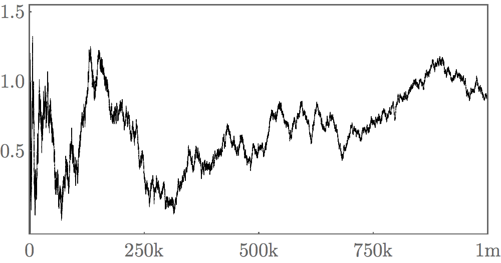
so Theorem 3 is an immediate corollary. Figure 1 shows values of the summatory function ${\bf A}_{n}(x)$ for the pentagonal number $-n=1$ (along with the asymptotic curve) and the non-pentagonal number $-n=-1$ .

Refer to caption — A ${\bf A}_{-1}(x)$ (solid black line) vs. $-\frac{12\sqrt{3}}{\pi^{2}}\sqrt{x}$ (dotted white line)

In the proof we will need to know the Petersson norm of the eta function, which is given by the next lemma.

Lemma 9.

We have $\|y^{\frac{1}{4}}\eta\|^{2}=\frac{\pi}{3\sqrt{6}}$ .

Proof.

For $\re(s)>1$ , let

E(\tau,s)=\sum_{\gamma\in\Gamma_{\infty}\backslash{\rm SL}_{2}(\mathbb{Z})}(\im\gamma\tau)^{s}

denote the nonholomorphic Eisenstein series (see, for example, [47]), and define

I(s):=\int_{{\rm SL}_{2}(\mathbb{Z})\backslash\mathbb{H}}E(\tau,s)y^{\frac{1}{2}}|\eta(\tau)|^{2}\,\frac{dxdy}{y^{2}}.

Since $E(\tau,s)$ has a pole at $s=1$ with residue $3/\pi$ , we have

\|y^{\frac{1}{4}}\eta\|^{2}=\operatorname*{Res}_{s=1}I(s).

On the other hand, we have

	$\displaystyle I(s)$	$\displaystyle=\int_{\Gamma_{\infty}\backslash\mathbb{H}}y^{s+\frac{1}{2}}\|\eta(\tau)\|^{2}\,\frac{dxdy}{y^{2}}$
		$\displaystyle=\sum_{n,m\geq 1}\left(\frac{12}{nm}\right)\int_{0}^{\infty}y^{s-\frac{1}{2}}e^{-2\pi(n^{2}+m^{2})\frac{y}{24}}\,\frac{dy}{y}\times\int_{0}^{1}e\left(\frac{n^{2}-m^{2}}{24}x\right)\,dx$
		$\displaystyle=\left(\tfrac{6}{\pi}\right)^{s-\frac{1}{2}}\Gamma(s-\tfrac{1}{2})\sum_{\begin{subarray}{c}n\geq 1\\ (n,6)=1\end{subarray}}\frac{1}{n^{2s-1}}=\left(\tfrac{6}{\pi}\right)^{s-\frac{1}{2}}\Gamma(s-\tfrac{1}{2})(1-\tfrac{1}{2})(1-\tfrac{1}{3})\zeta(2s-1).$

From this we obtain

\operatorname*{Res}_{s=1}I(s)=\frac{1}{\sqrt{6}},

as desired. ∎

Proof of Theorem 8.

By Proposition 1.2 of [44] and the discussion that follows, we see that the minimal eigenvalue of $\widetilde{\Delta}_{\frac{1}{2}}$ is $\lambda_{0}=\frac{3}{16}$ , so that $s_{0}=\frac{3}{4}$ . This is achieved by a unique normalized Maass cusp form in $L^{2}\left({\rm SL}_{2}(\mathbb{Z})\backslash\mathbb{H},\chi,\tfrac{1}{2}\right)$ , namely

(7.2)

u_{0}(\tau)=\frac{y^{\frac{1}{4}}\eta(\tau)}{\|y^{\frac{1}{4}}\eta\|}=\sqrt{\mathord{\raise 0.49991pt\hbox{$\displaystyle\genfrac{}{}{0.4pt}{}{3}{\pi}$}}}\,(6y)^{\frac{1}{4}}\eta(\tau).

Bruggeman studied families of modular forms on ${\rm SL}_{2}(\mathbb{Z})$ parametrized by their weight. His work [16, Theorem 2.15] shows that there are no exceptional eigenvalues in this case; in other words we have $\lambda_{1}>\frac{1}{4}$ . In forthcoming work [1] of the present authors we introduce a theta lift which gives a Shimura-type correspondence between the space in question and a space of weight $0$ Maass cusp forms of level 6. This, together with computations of Booker and Strömbergsson as in [12, Section 4] gives the lower bound $\lambda_{1}>3.86$ .

By Theorem 3 of [7] we can take $\beta=1/2$ . Proposition 7 and the bounds on $\lambda_{1}$ imply that

\sum_{c\leq x}\frac{S(m,n,c,\chi)}{c}=2\tau_{0}(m,n)x^{\frac{1}{2}}+O(x^{\frac{1}{6}+\epsilon}),

where (with $\widetilde{n}=n-\frac{23}{24}$ as before) we have

\tau_{0}(m,n)=2\sqrt{2i}\,\pi^{-\frac{1}{2}}\,\overline{\rho_{0}(m)}\rho_{0}(n)\widetilde{m}^{\frac{1}{4}}|\widetilde{n}|^{\frac{1}{4}}\Gamma\left(\tfrac{3}{4}+\tfrac{1}{4}\sgn(\widetilde{n})\right).

Equations (6.1), (6.2), and (7.2) give the relation

\sum_{m\in\mathbb{Z}}\rho_{0}(m)W_{\frac{1}{4}\sgn\left(\widetilde{m}\right),\frac{1}{4}}\left(4\pi\left|\widetilde{m}\right|y\right)e\left(\widetilde{m}x\right)=\sqrt{\mathord{\raise 0.49991pt\hbox{$\displaystyle\genfrac{}{}{0.4pt}{}{3}{\pi}$}}}\,(6y)^{\frac{1}{4}}q^{\frac{1}{24}}\left(1+\sum_{k=1}^{\infty}(-1)^{k}\left(q^{\frac{k(3k-1)}{2}}+q^{\frac{k(3k+1)}{2}}\right)\right).

Since

W_{\frac{1}{4},\frac{1}{4}}(y)=y^{\frac{1}{4}}e^{-y/2},

we find that

\rho_{0}(m)=\begin{cases}(-1)^{k}\sqrt{\mathord{\raise 0.49991pt\hbox{$\displaystyle\genfrac{}{}{0.4pt}{}{3}{\pi}$}}}\,6^{\frac{1}{4}}(4\pi\widetilde{m})^{-\frac{1}{4}}&\text{ if }m-1=\tfrac{k(3k\pm 1)}{2},\\ 0&\text{ otherwise.}\end{cases}

Therefore

\tau_{0}(m,n)=\begin{cases}(-1)^{k_{1}+k_{2}}\frac{6\sqrt{3i}}{\pi^{2}}&\text{ if }m-1=\tfrac{k_{1}(3k_{1}\pm 1)}{2}\text{ and }n-1=\tfrac{k_{2}(3k_{2}\pm 1)}{2},\\ 0&\text{ otherwise,}\end{cases}

and the theorem follows. ∎

References

[1] S. Ahlgren and N. Andersen, Kloosterman sums and Maass cusp forms of half integral weight for the modular group, Preprint, arXiv:1510.05191 [math:NT].
[2] S. Ahlgren and N. Andersen, Weak harmonic Maass forms of weight 5/2 and a mock modular form for the partition function, Res. Number Theory 1:10, 2015.
[3] S. Ahlgren, K. Bringmann, and J. Lovejoy, $\ell$ -adic properties of smallest parts functions, Adv. Math., 228(1):629–645, 2011.
[4] S. Ahlgren and B. Kim, Mock modular grids and Hecke relations for mock modular forms, Forum Math., 26(4):1261–1287, 2014.
[5] C. Alfes, Formulas for the coefficients of half-integral weight harmonic Maaß forms, Math. Z., 277(3-4):769–795, 2014.
[6] C. Alfes and S. Ehlen, Twisted traces of CM values of weak Maass forms, J. Number Theory, 133(6):1827–1845, 2013.
[7] N. Andersen, Singular invariants and coefficients of harmonic weak Maass forms of weight 5/2, Forum Math., to appear.
[8] G. E. Andrews, On the theorems of Watson and Dragonette for Ramanujan’s mock theta functions, Amer. J. Math., 88:454–490, 1966.
[9] G. E. Andrews, The number of smallest parts in the partitions of $n$ , J. Reine Angew. Math., 624:133–142, 2008.
[10] G. E. Andrews, F. G. Garvan, and J. Liang, Combinatorial interpretations of congruences for the spt-function, Ramanujan J., 29(1-3):321–338, 2012.
[11] A. O. L. Atkin and J. Lehner, Hecke operators on $\Gamma_{0}(m)$ , Math. Ann., 185:134–160, 1970.
[12] A. R. Booker and A. Strömbergsson, Numerical computations with the trace formula and the Selberg eigenvalue conjecture, J. Reine Angew. Math., 607:113–161, 2007.
[13] K. Bringmann, On the explicit construction of higher deformations of partition statistics, Duke Math. J., 144(2):195–233, 2008.
[14] K. Bringmann and K. Ono, The $f(q)$ mock theta function conjecture and partition ranks, Invent. Math., 165(2):243–266, 2006.
[15] K. Bringmann and K. Ono, An arithmetic formula for the partition function, Proc. Amer. Math. Soc., 135(11):3507–3514, 2007.
[16] R. W. Bruggeman, Modular forms of varying weight. III, J. Reine Angew. Math., 371:144–190, 1986.
[17] J. H. Bruinier, Borcherds products on O(2, $l$ ) and Chern classes of Heegner divisors, volume 1780 of Lecture Notes in Mathematics, Springer-Verlag, Berlin, 2002.
[18] J. H. Bruinier, Hilbert modular forms and their applications, in The 1-2-3 of modular forms, Universitext, pages 105–179, Springer, Berlin, 2008.
[19] J. H. Bruinier and J. Funke, On two geometric theta lifts, Duke Math. J., 125(1):45–90, 2004.
[20] J. H. Bruinier and J. Funke, Traces of CM values of modular functions, J. Reine Angew. Math., 594:1–33, 2006.
[21] J. H. Bruinier and K. Ono, Algebraic formulas for the coefficients of half-integral weight harmonic weak Maass forms, Adv. Math., 246:198–219, 2013.
[22] W. de Azevedo Pribitkin, Revisiting Rademacher’s formula for the partition function $p(n)$ , Ramanujan J., 4(4):455–467, 2000.
[23] M. Dewar and M. R. Murty, A derivation of the Hardy-Ramanujan formula from an arithmetic formula, Proc. Amer. Math. Soc., 141(6):1903–1911, 2013.
[24] NIST Digital Library of Mathematical Functions, http://dlmf.nist.gov/, Release 1.0.9 of 2014-08-29. Online companion to NIST Handbook of Mathematical Functions.
[25] L. A. Dragonette, Some asymptotic formulae for the mock theta series of Ramanujan, Trans. Amer. Math. Soc., 72:474–500, 1952.
[26] A. Folsom and K. Ono, Duality involving the mock theta function $f(q)$ , J. Lond. Math. Soc. (2), 77(2):320–334, 2008.
[27] A. Folsom and K. Ono, The $spt$ -function of Andrews, Proc. Natl. Acad. Sci. USA, 105(51):20152–20156, 2008.
[28] J. Funke, Heegner divisors and nonholomorphic modular forms, Compositio Math., 133(3):289–321, 2002.
[29] F. G. Garvan, Congruences for Andrews’ smallest parts partition function and new congruences for Dyson’s rank, Int. J. Number Theory, 6(2):281–309, 2010.
[30] F. G. Garvan, Congruences for Andrews’ spt-function modulo powers of $5$ , $7$ and $13$ , Trans. Amer. Math. Soc., 364(9):4847–4873, 2012.
[31] F. G. Garvan and C. Jennings-Shaffer, Hecke-type congruences for Andrews’ spt-function modulo 16 and 32, Int. J. Number Theory, 10(2):375–390, 2014.
[32] D. Goldfeld and P. Sarnak, Sums of Kloosterman sums, Invent. Math., 71(2):243–250, 1983.
[33] G. H. Hardy and S. Ramanujan, Asymptotic formulæ in combinatory analysis [Proc. London Math. Soc. (2) 17 (1918), 75–115], in Collected papers of Srinivasa Ramanujan, pages 276–309, AMS Chelsea Publ., Providence, RI, 2000.
[34] D. A. Hejhal, The Selberg trace formula for ${\rm PSL}(2,\,{\bf R})$ . Vol. 2, volume 1001 of Lecture Notes in Mathematics, Springer-Verlag, Berlin, 1983.
[35] H. Iwaniec, Topics in classical automorphic forms, volume 17 of Graduate Studies in Mathematics, American Mathematical Society, Providence, RI, 1997.
[36] N. V. Kuznetsov, The Petersson conjecture for cusp forms of weight zero and the Linnik conjecture. Sums of Kloosterman sums, Mat. Sb. (N.S.), 111(153):334–383, 1980.
[37] D. H. Lehmer, On the series for the partition function, Trans. Amer. Math. Soc., 43(2):271–295, 1938.
[38] K. Ono, Congruences for the Andrews spt function, Proc. Natl. Acad. Sci. USA, 108(2):473–476, 2011.
[39] W. d. A. Pribitkin, A generalization of the Goldfeld-Sarnak estimate on Selberg’s Kloosterman zeta-function, Forum Math., 12(4):449–459, 2000.
[40] H. Rademacher, On the partition function $p(n)$ , Proc. London Math. Soc., S2-43(4):241, 1936.
[41] H. Rademacher, Fourier expansions of modular forms and problems of partition, Bull. Amer. Math. Soc., 46:59–73, 1940.
[42] H. Rademacher, On the expansion of the partition function in a series, Ann. of Math. (2), 44:416–422, 1943.
[43] H. Rademacher, On the Selberg formula for $A_{k}(n)$ , J. Indian Math. Soc. (N.S.), 21:41–55 (1958), 1957.
[44] P. Sarnak, Additive number theory and Maass forms, in Number theory (New York, 1982), volume 1052 of Lecture Notes in Math., pages 286–309, Springer, Berlin, 1984.
[45] A. Weil, On some exponential sums, Proc. Nat. Acad. Sci. U. S. A., 34:204–207, 1948.
[46] A. L. Whiteman, A sum connected with the series for the partition function, Pacific J. Math., 6:159–176, 1956.
[47] D. Zagier, Eisenstein series and the Riemann zeta function, in Automorphic forms, representation theory and arithmetic (Bombay, 1979), volume 10 of Tata Inst. Fund. Res. Studies in Math., pages 275–301, Tata Inst. Fundamental Res., Bombay, 1981.
[48] D. Zagier, Elliptic modular forms and their applications, in The 1-2-3 of modular forms, Universitext, pages 1–103, Springer, Berlin, 2008.
[49] H. S. Zuckerman, On the coefficients of certain modular forms belonging to subgroups of the modular group, Trans. Amer. Math. Soc., 45(2):298–321, 1939.

Algebraic and transcendental formulas for the smallest parts functionThanks: The first author was supported by a grant from the Simons Foundation (#208525 to Scott Ahlgren).

Abstract.

1. Introduction

Theorem 1.

Theorem 2.

Example.

Theorem 3.

2. Preliminaries

2.1. Quadratic forms and Atkin-Lehner involutions

2.2. Quadratic spaces of signature (1,2)(1,2)

2.3. Harmonic Maass forms and the theta lift

3. Proof of the algebraic formula

Proposition 4.

Proof.

Remark.

Proof of Theorem 2.

4. Poincaré series and the function f⁡(τ)f(\tau)

Proposition 5.

Proof.

5. Proof of Theorem 1

Lemma 6.

Proof.

6. Sums of Kloosterman sums

Proposition 7.

7. Sums of Kloosterman sums for the η\eta-multiplier

Theorem 8.

Lemma 9.

Proof.

Proof of Theorem 8.

References

2.2. Quadratic spaces of signature $(1,2)$

4. Poincaré series and the function $f(\tau)$

7. Sums of Kloosterman sums for the $\eta$ -multiplier