Resource costs for fault-tolerant linear optical quantum computing

Numerous different physical systems have been explored as platforms for quantum information processing. Most approaches involve embodying information in matter systems such as ions or superconducting qubits, but a striking alternative is linear optical quantum computing (LOQC) where all information is encoded in electromagnetic field modes, and processing is carried out using only linear optical elements [1]. Using light as the information medium takes advantage of the low decoherence suffered by optical fields, and the relative ease with which quantum information can be encoded photonically. However there are drawbacks, in particular the impossibility of deterministic entanglement and the impact of photon loss (whether due to absorption, leakage or detector failure). Such difficulties can be solved by increasing the physical complexity of the circuitry. Thus while LOQC may benefit from simple building blocks, conversely it may require more complex circuits than other approaches, and the balance of these factors will determine whether the approach is a practical competitor to matter-based processors.

The most developed method for LOQC to date is based on a discrete dual-rail encoding, in which each qubit is encoded in the field modes occupied by a single photon [2] (these modes can be spatial, polarisation, time-frequency or any other degree of freedom supported by electromagnetic fields). Crucially, even though entangling operations between dual-rail encoded photonic qubits cannot succeed deterministically, it has been shown that it is nonetheless possible to build an essentially deterministic universal quantum computer using only linear optics. This can be achieved by attempting probabilistic entangling operations (PEO) between many resource states in order to ensure that, with high probability, a sufficient number of operations will succeed to allow for quantum computing [3, 4].

Techniques for mitigating photon loss have also been developed. It has been shown that if quantum information is suitably encoded in a multi-photon state, then losses of up to $50\%$ of the photons can be tolerated before the encoded information is lost [5]. However, in any realistic implementation of a quantum computer, one must account for how complex multi-photon states can be created given that every component, at every level, will be associated with finite rates of photon loss and other forms of noise. Furthermore, the circuitry associated with overcoming non-deterministic entanglement will require many linear optical elements, including delay lines and switching networks, in order to dynamically reroute the outputs of successful operations to the next stage of processing. These elements will induce further errors and losses, and in this sense the twin issues of non-deterministic entanglement and photon loss aggravate one another in LOQC. Fortunately the threshold theorem assures us that, if all physical error rates are sufficiently low then errors at the logical level can be made arbitrarily rare, and scalable fault-tolerant quantum computing can be achieved. The central challenge of quantum computing is therefore to demonstrate the operations necessary for quantum computing with error rates below these thresholds. Theoretical studies have established the required thresholds for architectures relevant to superconducting qubits [6], and to matter optical networks [7], and experimental systems have been demonstrated at, or beyond, the required performance levels [9, 10, 8]. However to our knowledge no prior paper has established requirements of LOQC at the per-component level while simultaneously tracking the overall resource costs.

In this paper, we propose a protocol for LOQC that includes every step from the initial generation of entanglement primitives to the deployment of a fully fault-tolerant scalable unit for quantum computing. We consider computational errors and losses at each stage and endeavour to employ the most efficient known protocols for optical quantum information processing. In contrast to previous studies of noise thresholds in optical quantum computing [11, 12], we explicitly account for the substantial resource costs of LOQC protocols. We focus on a purely linear optical network, without employing matter qubits as memories or for entanglement generation. However we do assume the availability of on-demand sources of single photons, without concerning ourselves with the particular method with which these would be generated [13]. It is important to recognise that our results only represent an upper bound on the physical characteristics that are required of the components in an LOQC system – our protocol can admit various further optimisations, and these will make the physical requirements less stringent. Nevertheless we believe the results we offer are highly relevant to the field, having been derived from protocols that are presently “state of the art”, and moreover it is therefore fair to compare the results here with those that have been derived for matter and hybrid matter-optical systems.

Our analysis allows us to make an estimate of the overall scale of the resources necessary to construct a fully fault-tolerant optical quantum computer. We choose the number of detectors as a metric for the device size, recognising that the total numbers for the other kinds of component will scale roughly proportionately. We find that one would require upwards of $10^{5}\text{ --- }10^{6}$ detectors per physically encoded qubit in the cluster state, therefore requiring a total of at least $10^{11}\text{ --- }10^{12}$ detectors to build a $1000$ logical qubit quantum computer ¹¹ 1 This assumes that each logical qubit will be encoded in a surface code consisting of $\sim 1000$ physical qubits [14].. Further, such a quantum computer would require loss rates per component below $\sim 10^{-3}$ and error rates below $\sim 10^{-5}$ per component.

Our protocol is based on a three-dimensional (3D) cluster state [15, 16, 17] [Fig. 1 (a)]. With the cluster state approach, all entanglement required by the quantum computation is generated ahead of the computation itself, which then proceededs purely through measurements. The 3D cluster states enables measurement-based implementations of topological quantum computing using the surface code [18, 19, 20], providing high thresholds for both qubit loss and computational errors [21]. Without qubit loss, 3D cluster states tolerate phase errors with a rate up to $3\%$ on each qubit; conversely, without computational errors, they tolerate up to $24.9\%$ qubit losses [21]; and with both computational errors and qubit loss, the threshold of errors decreases approximately linearly with the loss rate. Thus cluster states are particularly well suited to LOQC as they can be efficiently prepared with linear optics: there is no fundamental difficultly caused by a high rate of entanglement failure during the creation of the cluster state, provided that once it is created it surpasses these thresholds [3, 4, 22, 23].

The 3D cluster state is a graph state on a 3D lattice, which can be understood by supposing that each vertex on the graph denotes a qubit initialised in the state $|{+}\rangle$ and each edge denotes an controlled-phase gate entangling the two linked qubits. In the particular lattice we require, each qubit is connected to four neighbouring qubits, see Fig. 1(a). In order to create such a cluster state, our protocol requires one complete building-block state to be prepared for each eventual qubit in the cluster. Importantly, these building-block states contain sufficient redundant encoding that entanglement links between building blocks can be generated with a probability above that necessary for fault-tolerant computing. If suitable building blocks can be constructed, a fault-tolerant cluster state of arbitrary size can then be generated deterministically. We can therefore focus on the optimal approach to constructing these building-block states (Fig. 2), without concerning ourselves with the precise details of the 3D cluster state that will ultimately be generated. However, we note that it is only necessary to generate one 2D layer of the cluster state “at a time”, entangling it with the layer generated previously (each layer represents one ‘clock cycle’ of the computation, and therefore requires one vertex for every physical qubit). Therefore the building-block factories can be reused to generate each layer of the 3D cluster.

As in other cluster state generation protocols [3, 24, 25, 26, 27, 28, 29], our building-block state is also a graph state. We employ the star graph as the basic structure of our building blocks, Fig. 1 (a). This state is composed of one core qubit and several bridge units. While the core qubit is a single photonic qubit, each bridge unit is physically encoded in tree-structure graph state of several photonic qubits. In order to implement a PEO between two different building block states, a Bell measurement is carried out between the root qubits at the base of each bridge unit. The tree-like structure within the bridge units enables two key properties: In the case of a successful PEO between bridge units on two different building-block states, the core qubits on each building block become entangled, and the remaining qubits within each unit can be trimmed away, see the left part of Fig. 1 (b). Moreover, on failure of the entangling operation then the measurements on the remaining qubits within the bridge units allow us to identify any necessary phase correction to the core qubit, preventing its corruption (with high probability). The right part of Fig. 1 (b) summarises this protocol, see Appendix A for further details. This method for recovering from PEO failure via measurements on ancillary qubits follows the approach introduced in Ref. [5].

With these two properties, it is possible to make multiple attempts to form links between core qubits while still ensuring that errors remain below the fault-tolerant threshold. Two building blocks can therefore be successfully connected with a high rate provided that there are enough bridge units.

Since each core qubit must be linked to four other core qubits, the number of bridge units on the building blocks is chosen to be a multiple of four, with a quarter of the bridge units allocated for each connection. To establish an entanglement link, PEOs are performed on corresponding bridge unit in parallel. If there is one successful PEO and the removal measurements are also successful, then the connection is successfully established. If there is more than one successful PEO, we keep only one link. The connection fails if there are no successful PEOs or one of the removal operations fails. Connection failures are dealt with by treating core qubits with a failed connection as missing qubits [29], which can be tolerated by MBQC on the 3D cluster state.

The finally prepared state of core qubits is equivalent to the 3D cluster state up to some feedback single-qubit gates depending on outcomes of single-qubit measurements and Bell measurements for preparing the state. In the MBQC algorithm on the 3D cluster state, (core) qubits are measured in four bases, which are $\sigma^{x}$, $\sigma^{z}$, and $(\sigma^{x}\pm\sigma^{y})/\sqrt{2}$ (only for magic state injection). In our protocol, the feedback gate on a core qubit is always either the identity $\openone$ or the phase gate $\sigma^{z}$. Therefore, remarkably, core qubits can be measured before the cluster state is prepared! It is beneficial to do so, in order to reduce the effect of photon loss: core qubits are measured as early as possible, and obviously if a measurement fails then that particular building block is abandoned at its initial stage. Once the full feedback is known, we may update (flip) the recorded outcomes of any cores measured in $\sigma^{x}$ or $(\sigma^{x}\pm\sigma^{y})/\sqrt{2}$.

Each building-block state must be generated from an initial resource of unentangled single photons. In our scheme, these single photons are first entangled into three-qubit GHZ states. These entanglement primitives can then be sequentially combined into larger units using Bell measurements (Fig. 2). This process is known to be efficient for loss rates of less than 1/3 [30], since at each stage it is then possible increase (up to double) the size of the resulting entangled states. Further details on the building-block construction process are given in Appendix B.

Regardless of the specific architecture of the building block to be generated, this process requires two primary circuit elements. The first element, a GHZ-state factory, produces GHZ states probabilistically from single-photon inputs. The second element probabilistically joins two independent graph states into a larger graph state. Along with these two processing elements, it is also necessary to construct switching networks and delay lines in order to route photons between processing states. All of these operations must be realised using only linear optical elements, e.g. single-photon sources, beam splitters, switches, delay lines and photon detectors [Fig. 3 (a)].

In our scheme, we use the same GHZ-state factory as proposed in Ref. [30]. This circuit requires six single photon inputs, and, in the lossless case, successfully generates GHZ states with probability $1/32$ [Fig. 3 (b)]. Our fusion elements use Bell measurements as PEOs for joining intermediate states. These Bell measurements consume one photon from each input state [4]. A tempting alternative is to employ the Type-I fusion gate, which consumes only one photon and can also connect two graph states [4]. However, a Type-I fusion gate may convert photon loss into computational errors (see Appendix B), which should be avoided as overcoming errors is usually harder than overcoming photon loss. Therefore, we only use Bell measurements in our protocol [30]. The circuits we use for the Bell measurement are also shown in Fig. 3 (c). Without any ancillary resources, a linear optical Bell measurement (often termed Type-II fusion) can succeed with $50\%$ probability in the lossless case. However, with the help of four ancillary single photons, the success probability of a Bell measurement can be boosted to $75\%$ [31]. The same success probability can also be achieved with a Bell-state as the ancillary resource [32]. With a resource state of more entangled photons, the success probability can be further boosted [31, 32].

As neither GHZ-state generation nor Bell measurements can succeed deterministically, we select successful outcomes from these operations to feed into the next stage of construction. This requires a rapidly reconfigurable switchyard consisting of a network of switches. For example, to select $N$ successful copies of the three-qubit GHZ state from $M$ attempts in parallel, we need six $M$-input to $N$-output switchyards, one for each output mode of the GHZ-state generation circuit. Before photons enter switchyards, delay lines are necessary to allow time for the switchyard to be reconfigured.

We consider two different approaches to this switching requirement. In the ideal case, this switchyard would consist of a single reconfigurable switch with multiple inputs and outputs [33], in which there is no extra cost in terms of losses or errors as $N$ or $M$ increases. This may prove impossible to achieve, and so we also consider the opposite limit, in which a switchyard is built out of a network of $2$-to-$2$ switches. Such an $M$-to-$N$ switchyard can be realised with $M$ $1$-to-$N$ switchyards and $N$ $M$-to-$1$ switchyards [Fig. 3 (d)]. Each $1$-to-$N$ and $M$-to-$1$ switchyard is respectively composed of $\sim N$ and $\sim M$ $2$-to-$2$ switches, as also shown in Fig. 3 (d). With such a network of simple switches, each photon must go through approximately $\log_{2}(MN)$ switches. To minimise photon loss, switchyards with multiple inputs $M$ but a single output $N$ are favourable. However resources are not used efficiently in this case, and many successful PEO outputs will be discarded. To increase the efficiency, it is preferable to use switchyards with more output modes. In our numerical simulations, we have considered different configurations of the switch network to obtain the optimal threshold of a computer built with $2$-to-$2$ switches.

The main source of noise in LOQC is photon loss, which may be induced by any component on the optical path of the qubit. We assume that a loss occurs at single-photon sources, beam splitters, delay lines (for the time period required for one PEO stage), switches and detectors with the rates $p_{\text{e}}$, $p_{\text{b}}$, $p_{\text{d}}$, $p_{\text{s}}$ and $p_{\text{m}}$, respectively.

In addition to photon losses, we also have to consider computational errors. Because measurements are eventually attempted on all photonic qubits in the protocol, computational errors are induced by any source of noise that can affect these measurement outcomes. For example, any asymmetry, e.g. phase difference or biased transmission, between two modes of a qubit may result in computational errors. All computational errors are equivalent to Pauli errors (see Appendix C). In this paper, we assume that depolarising errors may happen at beam splitters, delay lines and switches with the rates $\epsilon_{\text{b}}$, $\epsilon_{\text{d}}$ and $\epsilon_{\text{s}}$, respectively. Imperfect modal overlap between different photon sources will lead to imperfect quantum interference at beam splitters, and therefore also to Pauli errors. For simplicity, in our model we incorporate this form of error into $\epsilon_{\text{b}}$.

Other types of noise are also tolerable in our protocol. For example, a photon source may emit two photons rather than a single photon into the circuit. Similar errors can be induced by switching errors, in which a photon enters the wrong mode, and from dark counts of detectors. To first order, all of these errors will be caught during measurement, since if these extra photons survive in the optical path we will measure more than the expected number of photons. In this case, we can simply treat the qubit as missing, an error which can be overcome in the same way as true photon loss. However, if a two-photon error is followed by a photon loss event, only one photon will be detected, and the measurement on such a qubit may give a wrong outcome. These computational errors are also equivalent to Pauli errors and can be corrected with our protocol. Although these errors can be corrected, we consider regimes in which they will occur at a rate much lower than the first-order error terms, and so we do not explicitly include them in our threshold study.

In this approach to LOQC, the fault-tolerance threshold depends on the complexity of each building-block state. With more resources, one can prepare bigger building blocks, and thus a higher level of photon loss is tolerable. In Fig. 4, fault-tolerant thresholds are obtained numerically (see Appendix D for details). In order to provide some physical intuition for the size of such linear optical quantum computers, we choose to specify the total number of detectors needed as our metric of the resources required. It can be seen that this approximately corresponds to twice the number of single photons needed, and therefore twice the number of single photon sources. It is likely that the resource burden of the other elements, e.g. beam splitters, delay lines and switches, will be of similar magnitudes.

Note that each curve in Fig. 4 (a) is actually an envelope representing the best of a very large number of protocols that were tested. Each small dot within the red curve in the upper left figure represents the outcome of one such simulation; these dots are omitted from other curves for clarity.

It is vital to appreciate that the number of detectors shown in the figure is for a single building-block state rather than the entire computer. A building-block state corresponds to only one qubit on the cluster state, i.e. one data qubit of the surface code, which could correspond to just one ion in an ion trap quantum computer or one superconducting qubit in a superconducting quantum computer. It is anticipated that a fault-tolerant quantum computer will need at least $\sim 10^{6}$ data qubits in order to be able to compete with state-of-the-art classical computers [14, 34]. We therefore do not consider building-block states with a resource requirement of greater than two billion detectors, since at that point one finds the entire computer requires thousands of trillions of components!

In Fig. 4 (a), we consider the case in which all components of the computer have the same photon loss rate. Depending on the choice of Bell measurement protocol, the threshold loss rate per component varies from $\sim 0.1\%$ to $\sim 0.2\%$. In this subfigure, we consider the worst case approach, in which each switchyard is built out of a cascade of $2$-to-$2$ switches. For comparison, in Fig. 4 (b) we consider a more sophisticated computer, in which each switchyard is a multiple-input multiple-output switch with the same loss rate as the other components. In this case the threshold is $\sim 3\text{ --- }5$ times higher than that of a simple-switch computer. We note that these thresholds approach the $1\%$ limiting loss rate that has been discussed in the context of a computing paradigm where gates are essentially deterministic but suffer a small probability of qubit loss [35] (we have achieved this at the cost of the additional resource overhead of course).

In order to further explore which components have the most significant impact on the fault-tolerance threshold, in Figs. 4 (c), (d), (e) and (f) we modify the model in Fig. 4 (a), assuming in each that one of the circuit components is lossless. These simulations confirm that it is the switching networks which most strongly impact the loss tolerance of the quantum computer. This suggests that alternative approaches in which intermediate cluster states are extensively recycled (similar to the recycling discussed in Ref [28]) will suffer from the associated increase in complexity of the switching networks.

The threshold changes dramatically with increased success probability Bell measurements. With a higher success probability, the size of building-block states (number of bridge units) can be smaller, hence both the level of noise and the resource cost can be lower. Bell measurements with $75\%$ success probabilities perform significantly better than those with $50\%$ success probability. Further, the single-photon ancilla assisted Bell measurement is slightly better than the Bell-state assisted Bell measurement. These boosted Bell measurements do however require photon detectors with additional photon-number resolution. In the case of the $50\%$-success Bell measurement, we need detectors that can distinguish photon numbers $0,1,2$, while for $75\%$-success Bell measurements, we need detectors that can distinguish photon numbers $0,1,2,3$. With more complex ancillary states, the success probability can be further boosted. However in this case more resources are required for preparing these ancillary states, which can counteract the benefits of the higher success probabilities (see Appendix E).

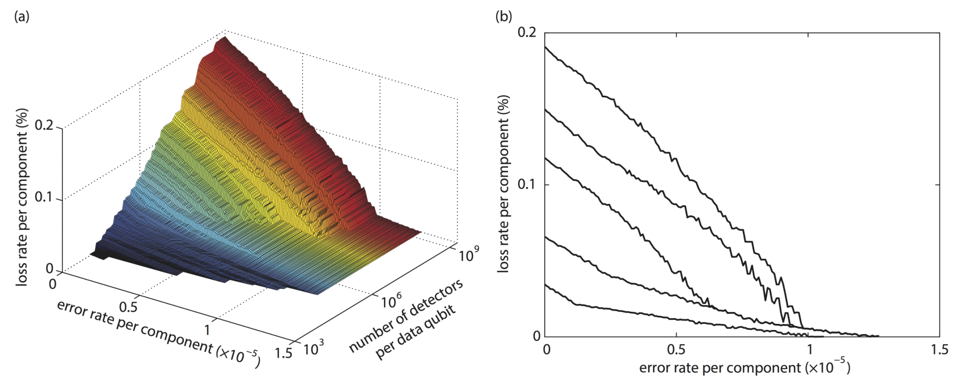
The presence of computational errors reduces the threshold loss rate. A general study of the threshold for both loss rates and error rates is shown in Fig. 5, in which we only consider quantum computers built with $2$-to-$2$ switches and single-photon ancilla assisted Bell measurements with $75\%$ success probability. More data for other Bell-measurement circuits and fancy switches can be found in Fig. 10. The threshold error rate per component is on the order of $10^{-5}$.

We have proposed a comprehensive protocol for LOQC with 3D cluster states, in which we consider the full network of linear optical devices necessary to realise a quantum computer. We find thresholds for loss and error rates of $\sim 10^{-3}$ and $\sim 10^{-5}$ per component, respectively. This per-component performance is beyond the current state of the art in photonics [38, 37, 36, 39, 41, 40, 42]. Furthermore we find that such a quantum computer would require on the order of $10^{11}$ detectors, and similar numbers of other components including deterministic and indistinguishable single photon sources. These component counts are several orders of magnitude greater than those required for systems with deterministic gates [14, 7].

We wish to emphasise that these stringent thresholds should be taken as a challenge to the community, aiming to stimulate further discussion and innovation in LOQC. From an experimental perspective, we have tried to determine which components will prove most critical in the development of an optical quantum computer. We found that, for our scheme, it is the performance of the optical switches that have by far the most impact the threshold loss and error rates, while other components contribute more equally. We hope that this will help guide the priorities of future experimental work aimed towards realising LOQC. From a theoretical perspective, we hope that our work will stimulate others to improve on our thresholds by exploring alternative schemes.