Solid-Supported Lipid Multilayers : Structure Factor and Fluctuations
Abstract
We present a theoretical description of the thermal fluctuations in a solid-supported stack of lipid bilayers, for the case of vanishing surface tension and in the framework of continuous smectic elasticity. The model is successfully used to model the reflectivity profile of a thin (16 bilayers) DMPC sample under applied osmotic pressure and the diffuse scattering from a thick (800 bilayers) stack. We compare our model to previously existing theories.
pacs
61.10.KwX-ray reflectometry (surfaces, interfaces, films) and 87.16.DgMembranes, bilayers, and vesicles and 87.15.YaFluctuations1 Introduction
Lipid bilayer systems have been extensively studied using X-ray techniques, including small-angle scattering and reflectivity measurements [1]. Among the various experimental configurations employed, the case of solid-supported stacks of bilayers is very important from a practical point of view, as these samples are amenable to powerful, interface-sensitive scattering techniques (specular and nonspecular scattering, grazing incidence difraction) avoiding the ambiguities associated with powder averaging [2, 3].
Besides the fundamental physical problems they raise, such as the molecular forces responsible for the inter-bilayer interaction potential (steric, electrostatic, van der Waals etc.); the influence of static defects; the loss of long-range order in low-dimensional systems and the role of the fluctuations, these systems can also serve as testing ground for the interaction of the cell membrane with membrane active molecules, such as antimicrobial peptides [4]. It is then of paramount importance to understand the different parameters influencing the scattering signal in order to achieve a comprehension of the spectra before the (sometimes subtle) effect of the included molecules can be confidently assessed.
One of the most characteristic hallmarks of lamellar systems (exhibiting one-dimensional order) is the Landau-Peierls effect, whereby the long-range order is destroyed by thermal fluctuations. Ever since the seminal paper of Caillé [5], this phenomenon has been studied in great detail, first in the bulk [6, 7, 8, 9, 10, 11, 12] and subsequently in thin films [13, 14, 15, 16], mainly under the influence of extensive experimental studies on freely-suspended films of thermotropic smectics (see [17] for a review). Recently, theoretical models were developed for the study of fluctuations in smectic films on solid substrates [18, 19], taking into account both the surface tension at the free surface and the boundary conditions imposed by the substrate.
In this paper we describe the thermal fluctuations in a solid-supported stack of lipid bilayers, concentrating on the (experimentally relevant) case of vanishing surface tension at the top of the stack. The influence of the substrate is only considered inasmuch as it limits the fluctuations of the bilayers, neglecting direct interactions (e. g. van der Waals, electrostatic) which can become important in the case of very thin films.
The paper is structured as follows : in section 2 we discuss the positional fluctuations of the layers in a solid-supported stack in the framework of continuous smectic elasticity, taking however into account the discrete nature of the system by the limitation of the number of modes along the normal direction. In contrast with (free-standing or supported) films of thermotropic smectics, for fully hydrated lipid multilayers the surface tension at the free surface vanishes. This greatly simplifies the theoretical treatment of the fluctuations. We conclude this section by a discussion of the in-plane variation of the correlation function.
Section 3 starts with a discussion of the specular structure factor . We then consider the influence on of the coverage rate, which can vary due to the preparation technique or to partial dewetting upon hydration. We compare our model with experimental data on the specular scattering and then with an estimate of the in-plane correlation function obtained from the diffuse scattering signal.
2 Smectic elasticity
We consider in the following a solid-supported sample with periodicity , of thickness and extending over a surface in the plane of the layers. We take the origin of the axis on the substrate, so that gives the position of the free surface. The in-plane position is denoted by .
2.1 Model and fluctuations
The simplest description of smectic elasticity is provided by the continuous smectic hamiltonian :
| (1) |
Following the treatment of Poniewierski and Hołyst [20], we shall decompose the deformation over independent modes; first, we take the Fourier transform of in the plane of the bilayer :
| (2) |
The free energy (1) can now be written as the sum , with :
| (3) |
The boundary conditions for the components are :
| (4a) | |||
| (4b) |
The first condition (4a) simply states that the fluctuations go to zero at the substrate; the second one (4b) is necessary in order to write in (3) as a quadratic form [14]. Physically, it expresses the continuity across the interface of the component of the stress tensor.
The correlation function of the fluctuations can be defined as :
| (5) |
where denotes the ensemble average. From the Wiener-Khinchin theorem, its Fourier transform is :
| (6) |
We then expand over the orthonormal set of harmonic functions , chosen to fulfill the boundary conditions (4) :
| (7) |
where the summation goes from to , instead of , because only components are required to describe the position of the bilayers (this amounts to restricting the summation to the first Brillouin zone). Keep in mind, however, that the index denotes here a particular deformation mode and not an individual bilayer.
Finally, the free energy can be written as a sum of independent modes : , where the ”stiffness” associated to each mode depends on the elastic constants , and . The equipartition theorem yields :
| (8) |
with the Kronecker symbol. Plugging (7) in (6), one has :
| (9) |
We can now Fourier transform back to the real space domain :
| (10) |
where is the in-plane distance (the symbol can safely be omitted).
2.2 The case of vanishing surface tension ()
Until now we have presented the general formalism; in each case, we must find the orthonormal set of functions , which are selected by the boundary conditions, and then determine the amplitude of each mode (or, equivalently, the stiffness ). This is what we shall now do for the case when , which is not only the simplest, but also the one relevant for systems of fully hydrated membranes [21].
The boundary conditions (4) are in this case : and , so the set of is :
| (11) |
The amplitudes are given by :
| (12) |
where , with . We also define the dimensionless parameter , first introduced by Caillé [5].
Finally, from equation (10) we have :
| (13) |

where the function can be expressed in terms of the Meijer G function11 1 It can be represented in Mathematica by the sequence : :
| (14) |
A first observation is that the fluctuation amplitude is always finite; the physical reason is that the presence of the substrate sets a lower boundary on the value of the wave vector in the direction : from equation (11), , thus forbidding the soft mode with and suppressing the Landau-Peierls instability. Hence, there is no need for a lower cutoff in the integral in equation (10).
It is immediately obvious that , so the correlation function for reduces to the simple formula :
| (15) |
which we shall use in determining the specular scattering of the sample (subsection 3.1). It is noteworthy that this function varies as for a fixed number of layers, so that any change in the thermodynamic parameter only results in a scale factor. This is very convenient for fitting the scattering spectrum of the system (see section 3), since the time-consuming calculation of the correlation matrix between the layers must only be performed once, and adjusting the and parameters only changes a prefactor.
As an illustration, we present in Figure 2 the values of the correlation function in a stack of 100 bilayers; in (a), represents the fluctuation amplitude for each bilayer, while in (b) represents the correlation of each bilayer with the one in the middle of the stack. Note the sigmoidal shape of the function in the first case and the very sharp peak in the second one.

Although for any finite number of layers the fluctuation amplitude of the top layer remains finite, it should diverge in the bulk limit . From formula (15) one obtains :
| (16) |
where is Euler’s constant and the digamma function is the logarithmic derivative of the gamma function, given by : . diverges logarithmically, being indistinguishable from as soon as .
The same divergence spuriously appears even for a finite when the stack is treated as a completely continuous medium, without limiting the number of modes to (formally, this amounts to letting and at fixed ). In this case, after summing over the modes, an artificial lower cutoff has to be introduced in the integral over , as in reference [14]. A comparison between our results and those obtained by this method is presented in the Appendix.
2.3 In-plane variation
We shall now consider the variation of the correlation function. At this point, it is convenient to introduce the correlation of the height difference defined by :
| (17) |
which has the advantage of remaining finite (for finite values of ) even in unbound systems. We shall further write the argument of the function in equation (13) as : , where emphasizing that, for a given number of layers, the variable in and scales with the correlation length . The physical significance of this quantity can be seen as follows [22] : for distances less than , the layers fluctuate independently, while for distances greater than the fluctuations are coherent from layer to layer. For an unbounded medium (translation invariance along ) it was shown [15] that, for the function behaves as
| (18) |
if and as
| (19) |
if . In the limit , diverges logarithmically, as it is well-known from the continuum theory [5].
We present in Figure 3 the height difference self-correlation function , computed from equations (17) and (13) for a stack of 800 bilayers.

In the low limit we find that, for all values of , is very well described by the asymptotic form (18). For high values of , the divergence (19) is replaced by saturation to a value of .
As we shall see in subsection 3.5, the self-correlation function can be extracted from the diffuse scattering signal; however, when also depends on this signal will be an average over the positions in the stack. For comparison with the experimental data we calculate (shown in Figure 3 as dotted line) as an average over for eight different values of , equally spaced from to .
3 Scattering
As discussed in the Introduction, notable differences appear between the scattering signal from bulk smectic phases and from solid-supported films. Even if the latter contain thousands of bilayers, the clear separation between specular and diffuse scattering shows that the Landau-Peierls effect is suppressed [23].
3.1 Specular scattering
In specular reflectivity studies, the incidence and reflection angles are equal : , corresponding to . As we shall see below, in this case only the correlation at zero in-plane distance (given by formula (15)) is relevant. For simplicity and to emphasize the discrete nature of the stack we shall use the notation .
The specular scattering factor of the lamellar stack (without taking into account the substrate) can be written as [29, 15] :
| (20) |
The spectra are corrected for the diffuse scattering by subtraction of an offset scan [2].

3.2 Accounting for partial dewetting
Fully-hydrated lipid multilayers differ from freely-suspended smectic films in that their thickness is not constant; partial dewetting leads to a variation in thickness over the area of the sample [24]. Notably, this leads to an obliteration of the Kiessig fringes, due to interference between the external interfaces of the system. We take this effect into account by introducing a coverage rate for each layer, , which is 1 at the substrate and decreases on approaching the free surface. The structure factor then reads :
| (21) | |||
For the coverage function we chose the convenient analytical form , where is an empirical parameter controlling the degree of coverage. This is a convenient method, but not a very precise one, insofar as the fluctuation spectrum is still calculated for a fixed number of layers, . In the limit where the size of the domains with a given thickness is larger than the X-ray coherence length, an alternative approach would be to incoherently (no cross-terms between domains) average over a distribution depending on the total layer number .
3.3 Describing the reflectivity profile
In order to model the reflectivity profile of our system, besides the structure factor of the stack one needs the form factor of the bilayers. Furthermore, the presence of the substrate must be taken into account. This is done using a semi-kinematic approximation, where the reflectivity of a rough interface is expressed by the master-formula of reflectivity [25] :
| (22) |
where denotes the Fresnel reflectivity of the sharp interface and is the intrinsic electron density profile whereas is the total step in electron density between the two adjoining media (silicon and water, in our case).
For the electronic density profile of the bilayer we use a parameterization in terms of Fourier components [2], which has the advantage of describing the smooth profile of lipid bilayers using only a few coefficients. For one bilayer we have :
| (23) |
where is defined between and , is the total number of Fourier components, is the amplitude of the -th component and the associated (complex) phase factor, which in our case can be shown to reduce to only, due to the mirror symmetry of the bilayers. The bilayer form factor is given by the Fourier transform of .
The total density profile is given by the density profiles of the bilayers (weighted by the coverage factors described in subsection 3.2) to which is added the profile of the substrate, described by an error function of width the rms roughness of the wafer (this quantity can be independently determined from the reflectivity of the blank wafer and is typically worth for all our measurements).
Effects related to the finite instrumental resolution and sample absorption are completely negligible in thin samples and were not implemented.
3.4 Comparison with experimental data
Lipid films partially hydrated in humid atmosphere exhibit many well-defined Bragg peaks, indicative of very low fluctuation amplitudes, so they are not a good testing ground for our model. On the other hand, samples hydrated in excess pure water sometimes have too few Bragg peaks. We thus chose to test our model against spectra obtained on samples that are in excess solvent, but under an osmotic pressure imposed by PEG (polyethylene glycol) solutions [26]. Fig. 5 shows the X-ray reflectivity of 16 1,2-dimyristoyl-sn-glycero-3-phosphocholine (DMPC) bilayers on a silicon substrate measured in an aqueous PEG solution of 3.6 wt. % concentration. The temperature was maintained at , at which the lipids are in the fluid phase. The continuous line shows a full -range fit to the data using the structure factor (21). From the position of the Bragg peaks one can determine a periodicity of . The suppression of the higher-order Bragg peaks clearly indicates the influence of the fluctuations. The fit yielded the parameters: for the Caillé parameter and for the coverage exponent in 21. The corresponding fluctuation amplitudes and coverage function are also shown. Further details on the results of these measurements will be presented elsewhere [26].

Experimental details : The curve in Fig. 5 was measured at the bending magnet beamline D4 at the HASYLAB/Desy in Hamburg, Germany. After the beam passed a Rh-Mirror to reduce high energy flux, a photon energy of was chosen using a single Si(111) crystal monochromator. The beam was collimated with several motorized vertical and horizontal slits. The reflected intensity was measured with a fast scintillation counter (Cyberstar, Oxford).
Sample preparation: The lipid 1,2-dimyristoyl-sn-glycero-3-phosphocholine (DMPC) was bought from Avanti and used without further purification. 16 bilayers were prepared on a commercial silicon substrate using the spin-coating method as described in [27]. The substrate was cut to a size of and carefully cleaned in an ultrasonic bath with methanol for ten minutes and subsequently rinsed with methanol and ultrapure water (Milli-Q, Millipore). The lipid was dissolved in chloroform at a concentration of . An amount of of the solution was pipetted onto the cleaned and dried substrate which was then accelerated to using a spin-coater. After rotation for 30 seconds, the sample was exposed to high vacuum over night in order to remove all remaining traces of solvent. The sample was refrigerated until the measurement. For the measurement the sample was mounted in a stainless steel chamber with kapton windows which can be filled and in situ flushed with fluids such as water or polymer solutions. PEG of molar weight 20.000 was bought from Fluka and used without further purification. A concentration of 3.6 wt. % corresponds to an osmotic pressure of about [28].
3.5 Diffuse scattering
It is well-known that the diffuse scattering signal from a surface can be expressed in terms of the height difference self-correlation function of the surface [29]. For a multilayer system, one must also take into account the cross-correlation function [30] and the calculations become much more complicated. However, it can be shown that by integrating the diffuse signal in over a Brillouin zone, the cross-correlation terms cancel and one is left with a curve corresponding to a transform of an average self-correlation function [31].
We compare our model to recent experimental data obtained on stacks of 800 fully-hydrated DMPC bilayers, where the experimental self-correlation function was obtained by inverting the integrated diffuse scattering [32]. In Figure 6 we present (open dots), as well as the function defined in subsection 2.3, with two different sets of fitting parameters and .

The theoretical curve can be scaled to the experimental data, either by adjusting both parameters, yielding for the Caillé parameter and (solid line in Fig. 6) or with a fixed parameter (from the analysis of the half width of the diffuse Bragg sheets [32]), and an open parameter which is adjusted to . Note that the present expression for can give better account of the experimental data than the bulk correlation function used before [15, 32]. In particular, it reproduces the observed saturation regime at high , while the bulk correlation function diverges logarithmically. However, systematic discrepancies between data and theory should not be overlooked. We note that the functional form of for small is not well captured, in particular it can not explain the exponent of the algebraic regime in the data. The possible reasons for this discrepancy can be manifold: contributions of non-bending modes to the diffuse scattering, a length scale dependent bending rigidity , residual tension in the bilayers due to edge effects, or nonlinearities in the Hamiltonian. This needs to be investigated in future studies. Finally, a more detailed treatment of the -dependence is needed, since the experimental analysis determines a correlation function which is averaged over the scattering volume.
4 Conclusion
The presence of a substrate dramatically changes the thermal fluctuations in lipid multilayers. Most noticeably, the Landau-Peierls instability is suppressed. We present a theoretical model taking into account this feature and show that it describes very well the experimental reflectivity data. Reasonable agreement is also obtained for the diffuse scattering. Our result is a first step towards a unitary interpretation of the global (specular and diffuse) scattering signal of solid-supported lipid multilayers.
Appendix. Comparison with previous results
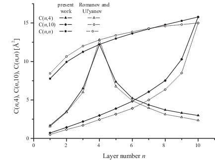
In order to assess the validity of our method, we compared our results with those obtained by Romanov and Ul’yanov by a rigorous treatment of the discrete model [19]. However, they only show data for smectic films with a rather high surface tension (). Thus, we chose their thickest film (21 layers) and only compared the values of for the bottom half (close to the substrate), where the surface tension plays a lesser role. As shown in Figure 7, the agreement is quite good.
We also compared our results to those obtained by Shalaginov and Romanov [14], who also used a continuous model, but without restricting the number of modes. For a solid substrate and a vanishing surface tension at the top, their equations (18a) and (22) lead to :
| (24) |
In Figure 8 we present our results for in a film with 61 layers, with and (solid dots) as well as the values obtained using the formula (24), for different values of the cutoff parameter (from top to bottom, 1.5, 4, 10, 30, 85, and 200 Å). Clearly, the fluctuation amplitude is very sensitive to the value of , with an approximately logarithmic dependence, and gives the same results as our method for . We remind that neither in our method, nor in the one of Romanov and Ul’yanov is there any need for a cutoff, due to mode number limitation (see the discussion in subsection 2.2).

Acknowledgements.
D. C. has been supported by a Marie Curie Fellowship of the European Community programme Improving the Human Research Potential under contract number HPMF-CT-2002-01903.References
- (1) J. Katsaras and V. A. Raghunathan, Aligned lipid-water systems, in Lipid bilayers : Structure and Interactions, edited by J. Katsaras and T. Gutberlet (Springer, 2000).
- (2) T. Salditt, C. Li, A. Spaar, and U. Mennicke, Europhys. J. E 7, 105-116 (2002).
- (3) Y. Lyatskaya, Y. Liu, S. Tristram-Nagle, J. Katsaras, and J. F. Nagle, Phys. Rev. E 63, 011907 (2000).
- (4) B. Bechinger J. Membrane Biol. 156, 197-211 (1997).
- (5) A. Caillé, C. R. Acad. Sci. Paris, Sér. B 274, 891-893 (1972).
- (6) J. Als-Nielsen, J. D. Litster, D. Birgenau, M. Kaplan, C. R. Safinya, A. Lindgard-Andersen, and S. Mathiesen, Phys. Rev. B 22, 312-320 (1980).
- (7) C. R. Safinya, D. Roux, G. S. Smith, S. K. Sinha, P. Dimon, N. A. Clark, and A.-M. Bellocq, Phys. Rev. Lett. 57, 2718-2721 (1986).
- (8) C. R. Safinya, D. Roux, G. S. Smith, Phys. Rev. Lett. 62, 1134-1137 (1989).
- (9) F. Nallet, R. Laversanne, and D. Roux, J. Phys II (France) 3, 487-502 (1993).
- (10) R. Zhang, R. M. Sutter, and J. F. Nagle, Phys. Rev. E 50, 5047-5060 (1994).
- (11) J. F. Nagle, R. Zhang, S, Tristram-Nagle, W. Sun, H. I. Petrache and R. M. Suter, Biophys. J. 70, 1419-1431 (1996).
- (12) G. Pabst, M. Rappolt, H. Amenitsch, and P. Laggner, Phys. Rev. E 62, 4000-4009 (2000).
- (13) R. Hołyst, Phys. Rev. A 44, 3692-3709 (1991).
- (14) A. N. Shalaginov and V. P. Romanov, Phys. Rev. E 48, 1073-1083 (1993).
- (15) N. Lei, C. R. Safinya and R. F. Bruinsma, J. Phys. II France 5, 1155-1163 (1995); N. Lei, Ph. D. Thesis, Physics Department, Rutgers, The State University of New Jersey (1993).
- (16) E. A. L. Mol, J. D. Shindler, A. N. Shalaginov and W. H. de Jeu, Phys. Rev. E 54, 536-549 (1996).
- (17) P. Oswald and P. Pieranski, The Liquid Crystals : Concepts and Physical Properties Illustrated by Experiments (in French), (CPI, Paris, 2002).
- (18) D. K. G. de Boer, Phys. Rev. E 59, 1880-1886 (1999).
- (19) V. P. Romanov and S. V. Ul’yanov, Phys. Rev. E 66, 061701 (2002).
- (20) A. Poniewierski and R. Hołyst, Phys. Rev. B 47, 9840-9843 (1993).
- (21) S. A. Safran, Adv. Phys. 48, 395-448 (1999).
- (22) W. Helfrich, Z. Naturforsch. A 33, 305-315 (1978).
- (23) T. Salditt, C. Münster, J. Lu, M. Vogel, W. Fenzl, and A. Souvorov, Phys. Rev. E 60, 7285-7289 (1999).
- (24) L. Perino-Gallice, G. Fragneto, U. Mennicke, T. Salditt, and F. Rieutord, Europhys. J. E 8, 275-282 (2002).
- (25) J. Als-Nielsen and D. McMorrow, Elements of Modern X-Ray Physics, (Wiley, Chichester, 2001).
- (26) U. Mennicke, D. Constantin, and T. Salditt, in preparation.
- (27) U. Mennicke and T. Salditt, Langmuir 18, 8172-8177 (2002).
- (28) The data was obtained from the web site of the Membrane Biophysics Laboratory at the Brock University in Canada : http://aqueous.labs.brocku.ca/osfile.html. The value for the osmotic pressure induced by a PEG 20000 solution at 3.6 wt. % is only available at as . At , temperature at which the experiments were performed, we estimate that the pressure is lower by about 10 to 20 %, by using the temperature dependence of PEG 8000 solutions (available on the same site).
- (29) S. K. Sinha, E. B. Sirota, S. Garoff, and H. B. Stanley, Phys. Rev. B 38, 2297-2312 (1988).
- (30) S. K. Sinha, J. Phys. (France) III 4, 1543-1557 (1994).
- (31) T. Salditt, T. H. Metzger, and J. Peisl, Phys. Rev. Lett. 73, 2228-2231 (1994), T. Salditt, T.H. Metzger, Ch. Brandt, U. Klemradt, and J. Peisl, Phys. Rev. B 51, 5617-5627 (1995).
- (32) T. Salditt, M. Vogel, and W. Fenzl, Phys. Rev. Lett. 90, 178101 (2003).