Effective mass theory for the anisotropic exciton in 2D crystals: Application to phosphorene
Abstract
We present a theoretical study of the exciton binding energy for anisotropic two-dimensional crystals. We obtain analytical expressions from variational wave functions in different limits of the screening length to exciton size ratio and compare them with numerical solutions, both variational and exact. As an example, we apply these results to phosphorene, a monolayer of black phosphorous. Aided by density functional theory calculations for the evaluation of the two-dimensional polarizability, our analytical solution for the exciton binding energy gives a result which compares well with numerical ones and, in turn, with experimental values, as recently reported.
I Introduction
Since the mechanical exfoliation of graphene[1], research in understanding the properties of two-dimensional (2D) crystals has increased in many folds. Atomically thin single-layered materials obtained from transition metal dichalcogenides[2], boron nitride[3], bismuth[4], etc. are being extensively studied for applications as electronic and photoelectronic devices. Few-layered black phosphorous (BP) is a recent addition to the list of graphene-inspired materials[5, 6, 7, 8]. Apart from having a sizeable band gap which can be tuned by the manipulation of the number of layers, the atomic structure of BP is highly anisotropic which leads to high asymmetry of the electronic band structure even for few layers. In particular, a single layer of BP or phosphorene is attracting most of the attention. The peculiar anisotropic nature of the band gap distinguishes phosphorene from other 2D crystals, increasing its potential functionality.
Excitons are a bound state of an electron and an hole and play an important role in the optical properties of the material. Understanding the nature of excitons and their dependence on the electronic structure of the host material is critical and lends a deeper perspective into the many-body physics involved in 2D crystals. The 2D nature of the polarizability of these crystals introduces an important length scale (screening length) . For distances between charges in the crystal plane, , greater than the electron-hole binding potential behaves like in a 3D system i.e., it goes as . However, for the case where is less than the potential is 2D-like, i.e., logarithmic. This behavior makes excitons in 2D crystals different from their 3D counterparts[9, 10].
Since most common 2D crystals are isotropic, the effect of anisotropy on the optical properties of these materials has remained essentially unexplored. The appearance of phosphorene has, however, changed this view and recent works address this issue from an analytical[8], numerical[11], and first-principles[7] standpoints. Here we give a detailed account of a variational approach, introduced by us in Ref. 8, to the calculation of the exciton binding energy in anisotropic 2D crystals. Several analytical expressions are derived in certain limits of the 2D interaction potential. The accuracy of our analytical expressions for is tested against both variational and exact numerical solutions to the actual 2D potential, finding excellent agreement in a wide and experimentally relevant range of screening lengths. In particular, the value of for phosphorene, as obtained from our analytical expression, compares almost exactly to the numerical results. Furthermore, this value nicely agrees with the recently reported experimental result[12].
The present work is divided as follows. In Sec. II we review the form and limiting behaviour of the Coulomb interaction potential for charged particles in 2D systems. In Sec. III we present our variational approach based on an anisotropic exciton wavefunction. We first present the analytical result for in the limiting case where the 2D potential reduces to the standard 3D Coulomb potential for isotropic 2D systems to later introduce the anisotropy and re-derive the binding energy for this case. In the same manner we derive analytical expressions for the isotropic and anisotropic binding energies in the opposite limit where the 2D interaction potential behaves logarithmically. We also compare our analytical expressions with the numerically solved variational problem as well as with the exact numerical solution. In Sec. IV we propose an alternative variational approach based on gaussian orbitals. In Sec. V, after computing the 2D polarizability with density functional theory (DFT), our analytical approach is applied to the case phosphorene. Finally we present our conclusions in Sec. VI.
II Binding particle-hole potentials in 2D
As originally derived by Keldysh[13], the Coulomb potential energy created by a point charge at the origin that electrons feel in 2D layers follows the expression:
| (1) |
where and . Here is the thickness of the 2D material, is its bulk dielectric constant, and and are the dielectric constants of the surrounding media, typically substrate and vacuum. Here plays the role of a screening length and sets the boundary between two different behaviours of the potential. For the potential diverges logarithmically, as if created by line charges. In this limit, the potential takes the simplified form also given by Keldysh[13]:
| (2) |
where is the Euler constant. For the potential becomes the standard Coulomb potential created by point charges which decays as :
| (3) |
A very good approximation to the Keldysh potential, fairly accurate in both limits and simpler to use, was introduced by Cudazzo et al.[9]:
| (4) |
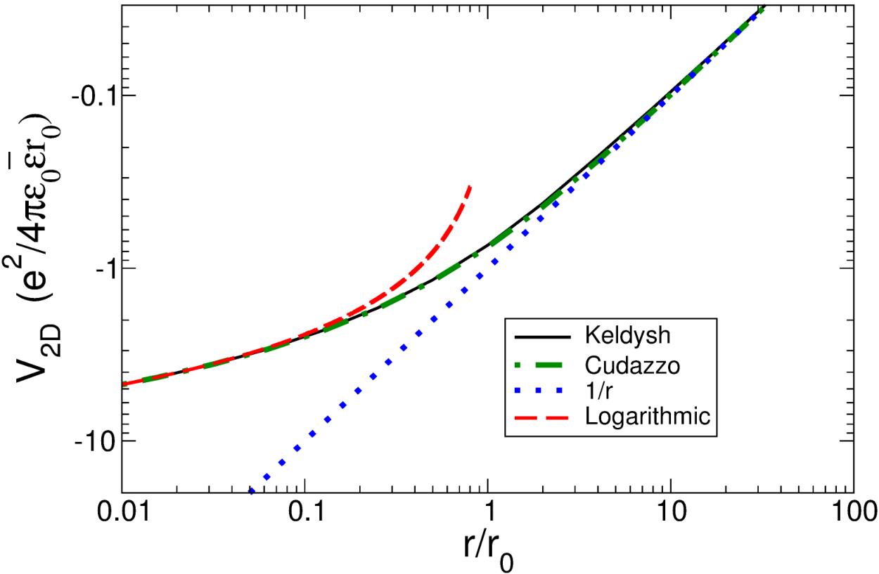
It is interesting to compare these four expressions as a function of the distance in a range of several orders of magnitude both above and below . We present such a comparison in Fig. 1. There it can seen the range of validity of each approximation, the Cudazzo et al. expression being remarkably accurate for all distances.
III variational wavefunction approach
For generic 2D crystals with electrons and holes presenting anisotropic effective masses, , we consider variational solutions for the exciton wave function of the type[14]:
| (5) |
where is the variational anisotropy scaling factor relating the exciton extension along the direction, (which is also a variational parameter) and the one along the direction (). With this variational wavefunction we can evaluate the expectation value of the kinetic energy:
where and are the reduced effective masses, , along and directions, respectively. The expectation value of the potential energy is given by
| (6) |
and the variational exciton binding energy is obtained from the addition of these two quantities,
| (7) |
Upon minimization with respect to and , one obtains the optimal parameters defining the extension and shape of the exciton and the actual binding energy . Results from three minimization procedures, one analytical and two numerical, are presented in next section.
III.1 Analytical Results
The integral for the potential energy in Eq. (6) turns out to be too difficult for an exact variational analytical solution. The main goal of this section is to make use of the asymptotic behaviour of the Keldysh potential to get analytical expressions for in the limits and , namely, valid for large and small excitons, respectively.
III.1.1 limit
We begin by evaluating in the isotropic case (, ), considering only the long-range behaviour of the Keldysh potential (see Eq. 3). The contribution of the potential energy to is given in this limit by
| (8) |
Now minimizing with respect to the variational exciton radius one obtains
| (9) |
where the minimal exciton radius is given by
| (10) |
and and are the free electron mass and the Bohr radius, respectively.
For the anisotropic case () the exciton extension along the -direction is now given by
| (11) |
In the previous expression we find a function of defined through the elliptic integral
| (12) | |||||
where the function K is the complete elliptic integral of the first kind. Defining now as
| (13) |
the exciton extension along the axis can now be written as
| (14) |
The exciton extension along the direction is thus
| (15) |
and the -dependent binding energy of the exciton now becomes
| (16) |
We now define
| (17) | |||||
where E is the complete elliptic integral of second kind. We can see that the minimal , , satisfies in general the following equation:
| (18) |
which has no analytical solution for . However, it can be shown [14] that for
| (19) |
Finally, notice that the results obtained in this subsection will be valid as long as the exciton extension in both and directions is much larger than . The consistency of this approximation for given experimental parameters (, , , and ) has to be checked a posteriori.
III.1.2 limit
As the logarithmic behaviour of the Keldysh potential dominates. The potential energy in 2D takes now the form given in Eq. (2). In the isotropic case the exciton radius is now given by
| (20) |
and the binding energy of the exciton is
| (21) |
For an anisotropic system the -dependent exciton extension along the direction is given by
| (22) |
Using now a different definition for
| (23) |
the exciton -extension now becomes
| (24) |
Again, taking into account that , the -dependent minimal exciton extension along the direction is
| (25) |
Note that .
Finally we obtain the exciton energy for this case:
| (26) |
where the minimal is
| (27) |
for all and . Again, notice that this result will be valid as long as the and minimal extensions of the excitonic wave function are small compared to .
Note that Eq. (26) can be written in a more symmetrical way as a function of both and ,
and that it is also symmetrical under exchange of and , as it should be. However, we find that the binding energy is not only a function of , but depends on both their values.
Finally, for completeness, we present an analytical expression for the exciton binding energy using the Cudazzo potential in the isotropic case:
| (28) |
where is the exponential integral function. We have only been able to obtain a working analytical expression for (too cumbersome to be shown here) in the limit where the above expression is actually useful.

III.2 Numerical Optimization and exact solution


To validate and test the accuracy of the limiting analytical expressions given in the previous section, we now use the wavefunction in Eq. (5) to numerically compute the potential energy given by Eq. (6) for the exact Keldysh potential. We also solve, numerically as well, the 2D Schrödinger equation for the same potential, which will give us the exact value of (down to the required numerical precision). Exciton binding energies for the isotropic case () are presented in Fig. 2 as a function of the screening length . For comparison’s sake, we take , i.e., the 2D crystal is suspended in vacuum, and . Thus, according to Eq. (9), Ryd (where Ryd is the Rydberg energy eV) for . The numerical variational result compares very well with the exact numerical value in the large range of explored screening lengths. For the analytical solution in Eq. (21) works fairly well. There, the size of the exciton is smaller than and the contribution to the Keldysh potential is negligible. As expected, the analytical solution starts to fail as since there the size of the exciton becomes comparable to and the long-range contribution to the Keldysh potential becomes dominant. (One should keep in mind that the limit of validity of the analytical result, as shown in Eq. (20), depends on the values of and .) We also compare with the result given by Eq. (28), obtained using the approximate expression to the potential in Eq. (4). This expression, although not as friendly as the previous one, extends the limit of validity of our analytical results down to .
The results for the anisotropic case are presented in Fig. 3 for and as a function of the anisotropy ratio with (notice a difference of one order of magnitude in the energy scales of each plot). Note that these curves would be identical if plotted as a function of with . Once again there is close agreement between the analytical solution [Eq. (26)], the numerical optimization, and the exact numerical solution for large , while for the smaller value, the analytical solution visibly deviates from the other two.
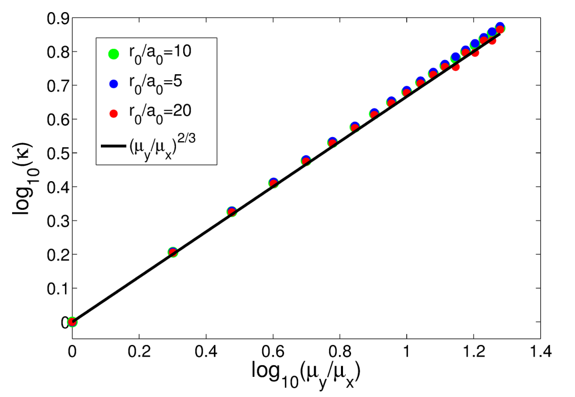
An important prediction of our analytical results is the relation between the anisotropy in the exciton extension and the effective masses: , which becomes exact in the limit of small excitons. To test this relation we fitted the optimal value of the variational parameter to the law
| (29) |
for a large range of . The results of this fit are presented in Fig. 4. They confirm our analytical results and recover the exact 1/3 exponent in the limit of large .

We finally provide a comparison between the exact and variational wave functions for several values of in the isotropic limit (see Fig. 5). Note that the distance is rescaled with the optimal radius and the amplitude of the wave function with the normalization constant .This representation illustrates to what extent the exact and variational wave functions satisfy similar scaling relations. Note that at the exact wave functions do not show the prominent cusp of a 1s Slater-type orbital. This softened behavior at the origin suggests than a combination of gaussian functions may capture more accurately this feature of the wave function, as shown in next section.

IV Gaussian-Basis Variational Method
We have found that in the limit of very small , the binding energy is very sensitive to small changes in . Furthermore, the numerical solution of the Schrödinger equation requires a very fine mesh to reproduce the bound state in such a limit. On the other hand, the analytical result found in the limit of the potential constitutes an isolated point an thus cannot be easily extended to small but finite values of . It is therefore interesting to find an alternative numerical method to study anisotropic excitons in the limit of small . Moreover, as we have presented in Fig. 5, the behavior of the exciton exact wave functions for different values of the screening length resembles more a 1s Gaussian than a Slater-type orbital. Gaussian-type orbitals (GTO) are very efficient basis sets used intensively in quantum chemistry and solid state calculations.
The gaussian basis functions follow the expression:
| (30) |
The index is an integer that here has been chosen to run from 1 to 4 and the exponents are coefficients that have to be optimized to minimize the ground state energy obtained by the variational method. Unlike the conventional gaussian approach, the anisotropy of the problem introduces two coefficients per GTO. We limit the variational freedom assuming that the anisotropy is identical for the four basis functions:
| (31) |
In this equation, is a constant that does not depend on so that we reduce the number of exponents that we have to optimize from eight to four. The variational wave function in the GTO basis is given by
| (32) |
For fixed values of , the energy is computed by generalized diagnonalization of a 4x4 matrix. The matrix elements of the kinetic energy are
| (33) |
The matrix elements of the potential energy are computed by numerical integration,
| (34) |
and the overlap matrix is
| (35) |
where .
The binding energy and the optimal wave function are obtained by minimizing numerically the energy with respect to the five variational parameters. Efficient optimization of the energy requires a careful choice of the initial guess for the values of the exponents . In our case, we choose the optimal values for a 1s orbital of a “2D hydrogen atom”, taking and approaching zero. Once these optimal exponents are obtained, is changed slightly and the problem is solved again, using this time the exponents obtained in the previous step. The procedure continues until the ground state energy for the desired is reached.
For example, fixing and , the effective mass along the axis is varied from 1 to 40. In this case the initial guess for the exponents is the last set of coefficients obtained when changing . The result for the ground state energy of this calculation is shown in Fig. 6 in comparison to the numerical solution of the Schrödinger equation with the Keldysh potential. They match perfectly. Two other values of obtained with the same gaussian-basis variational method are also shown.

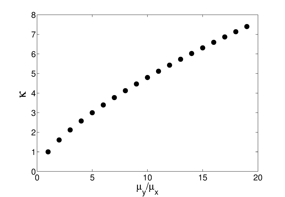
In Fig. 7, the length scales of the whole set of optimal GTO’s for are plotted vs for . is also plotted in Fig. 8 against the same quantity. In Fig. 9 we show a log-log representation of versus the asymmetry ratio for different values of where a linear fitting has been made.

V Application to phosphorene
A paramount example of an anisotropic 2D crystal is phosphorene[5, 6, 8], where the effective masses along and directions can differ by even an order of magnitude. From the start we have chosen to express the 2D potential constant in terms of the bulk dielectric constant and the effective thickness of the 2D crystal (see Eq. 1). Equivalent expressions for the 2D potential, which rely on the evaluation of the actual 2D polarizability of the 2D crystal, , have recently been proposed[9, 10, 11]. These are probably more appropriate for actual crystals, although it has also been shown that Eq. (1) works well as long as is taken as the in-plane component of the bulk dielectric tensor[10] of the 3D crystal. Here we will compare both possibilities.
As shown in Ref. 9, the screening length depends on the polarizability as . The polarizability for 2D materials can be computed using the expression
| (36) |
where is the distance between layers in a 3D layered structure. As can be seen, the dielectric function tends to unity as the inter layer distance tends to infinity. We have computed the dielectric function at different inter layer distances within the density functional theory framework using the Perdew-Burke-Ernzerhof (PBE) functional[15] and norm conserving Troullier-Martins (TM) pseudopotentials as available in the SIESTA package[16]. The atomic and electronic structures have been duly converged on all parameters. SIESTA calculates the imaginary part of the dielectric function from which the real part of it is obtained using the Kramers-Kronig relations. In order to account for the under-estimated band gap, the scissor approximation, as implemented in SIESTA, has been utilized. The scissor shift of 1.2505 eV was made to match our previously reported band gap value of 2.15 eV[8]. While more elegant approaches to the gap problem of phosphorene have been reported in the literature[7], the scissor approximation suffices to our purpose here.


Using the plane-averaged static dielectric function calculated with SIESTA (see Fig. 10), a value in the vicinity of of 3.8 Å is obtained. This value for yields a screening length of Å. From the numerical variational solution we obtain an exciton extension of Å and Å along the x and y directions, respectively. Since these values are smaller than , the use of the analytical expressions obtained in the logarithmic limit of the potential is justified. Also this was expected from Fig. 2 and, in particular, from the comparison shown in Fig. 3 for anisotropic cases. There it can be seen that already for the deviation between the analytical result and the numerical ones is less than 10% for a ratio (which corresponds to phosphorene). Using now Eqs. (22)–(27), we obtain an exciton binding energy for phosphorene in vacuum of eV, while the numerical variational value is eV. This result is remarkably close to a recently reported experimental value of eV. The agreement is somewhat surprising since this has been measured for phosphorene on a SiO substrate[12]. A more recent experiment, however, reports a smaller value for , which is maybe more expected due to the screening of the substrate[17].
Similarly, we can use the value of obtained from the real part of the bulk (at zero frequency) and the thickness of the monolayer. Since the thickness is somewhat undetermined, we have computed the binding energy for varying , as shown in Fig. 11. It can be observed that the binding energy of the monolayer computed using the microscopically derived matches the binding energy obtained using for Å, which certainly can be considered the thickness of phosphorene.

VI conclusions
We have shown that a variational approach to the exciton binding energy in anisotropic 2D crystals can give excellent results when compared to numerical approaches. Furthermore, we have studied the range of validity of analytical solutions to the variational approach and found that these can give highly satisfactory results in a range of values of screening lengths which is relevant for actual 2D crystals such as phosphorene. We have computed the exciton binding energy in this case and found a very good agreement with a recently reported experimental result[12]. As long as the screening length to exciton size is large, our analytical results can be trivially used to predict the exciton binding energy of any 2D crystal.
Acknowledgements.
This work was supported by MINECO under Grants Nos. FIS2013-47328 and FIS2012-37549, by CAM under Grants Nos. S2013/MIT-3007, P2013/MIT-2850, and by Generalitat Valenciana under Grant PROMETEO/2012/011. The authors thankfully acknowledge the computer resources, technical expertise, and assistance provided by the Centro de Computación Científica of the Universidad Autónoma de Madrid. E.P. also acknowledges the Ramón y Cajal Program.References
- [1] K. S. Novoselov, A. K. Geim, S. V. Morozov, D. Jiang, Y. Zhang, S. V. Dubonos, I. V. Grigorieva, and A. A. Firsov, Science 306, 666 (2004).
- [2] J. N. Coleman, M. Lotya, A. O’Neill, S. D. Bergin, P. J. King, U. Khan, K. Young, A. Gaucher, S. De, R. J. Smith, I. V. Shvets, S. K. Arora, G. Stanton, H.-Y. Kim, K. Lee, G. T. Kim, G. S. Duesberg, T. Hallam, J. J. Boland, J. J. Wang, J. F. Donegan, J. C. Grunlan, G. Moriarty, A. Shmeliov, R. J. Nicholls, J. M. Perkins, E. M. Grieveson, K. Theuwissen, D. W. McComb, P. D. Nellist, and V. Nicolosi, Science, Volume 331, Issue 6017, pp. 568- (2011). 331, 568 (2011).
- [3] M. Kawaguchi, S. Kuroda, and Y. Muramatsu, Journal of Physics and Chemistry of Solids 69, 1171 (2008), 14th International Symposium on Intercalation Compounds ISIC 14.
- [4] C. Sabater, D. Gosálbez-Martínez, J. Fernández-Rossier, J. G. Rodrigo, C. Untiedt, and J. J. Palacios, Phys. Rev. Lett. 110, 176802 (2013).
- [5] L. Li, Y. Yu, G. J. Ye, Q. Ge, X. Ou, H. Wu, D. Feng, X. H. Chen, and Y. Zhang, Nature Nanotechnology, Volume 9, Issue 5, pp. 372-377 (2014). 9, 372 (2014).
- [6] H. Liu, A. T. Neal, Z. Zhu, Z. Luo, X. Xu, D. Tománek, and P. D. Ye, ACS Nano 8, 4033 (2014).
- [7] V. Tran, R. Soklaski, Y. Liang, and L. Yang, Physical Review B, Volume 89, Issue 23, id.235319 89, 235319 (2014).
- [8] A. Castellanos-Gomez, L. Vicarelli, E. Prada, J. O. Island, K. L. Narasimha-Acharya, S. I. Blanter, D. J. Groenendijk, M. Buscema, G. A. Steele, J. V. Alvarez, H. W. Zandbergen, J. J. Palacios, and H. S. J. v. d. Zant, 2D Materials 1, 025001 (2014).
- [9] P. Cudazzo, I. V. Tokatly, and A. Rubio, Phys. Rev. B 84, 085406 (2011).
- [10] T. C. Berkelbach, M. S. Hybertsen, and D. R. Reichman, Phys. Rev. B 88, 045318 (2013).
- [11] A. S. Rodin, A. Carvalho, and A. H. Castro Neto, Physical Review B, Volume 90, Issue 7, id.075429 90, 075429 (2014).
- [12] X. Wang, A. M. Jones, K. L. Seyler, V. Tran, Y. Jia, H. Zhao, H. Wang, L. Yang, X. Xu, and F. Xia, Nat. Nanotechnology 10, 517 (2015) .
- [13] L. V. Keldysh, JETP Lett. 29, 658 (1979).
- [14] A. Schindlmayr, European Journal of Physics, Volume 18, Issue 5, pp. 374-376 (1997). 18, 374 (1997).
- [15] Y. Zhang and W. Yang, Physical Review Letters, Volume 80, Issue 4, January 26, 1998, p.890 80, 890 (1998).
- [16] J. M. Soler, E. Artacho, J. D. Gale, A. García, J. Junquera, P. Ordejón, and D. Sánchez-Portal, Journal of Physics: Condensed Matter 14, 2745 (2002).
- [17] J. Yang, R. Xu, J. Pei, Ye W. Myint, F. Wang, Z. Wang, S. Zhang, Z. Yu, and Y. Lu, “Optical tuning of exciton and trion emissions in monolayer phosphorene,” (2015), arXiv:1504.06386.