Quantum statistics and the performance of engine cycles

Let us consider a process from Hamiltonian parameter $\omega_{a}$ to $\omega_{a}^{\prime}$. The respective single particle $j$-th energy eigenvalues will be $\varepsilon_{j}$ and $\varepsilon^{\prime}_{j}$. Let $n_{j}$ represent the number of particles in the $j$-th single energy eigenstate.

A single $N-$body state is thus given by the ordered set of occupation numbers $\{n_{j}\}$. A process is performed quasi-statically by changing the trap parameter adiabatically, and the corresponding $N-$body microstate at the end of the compression is then given by $\{m_{k}\}$. For a single realization of the protocol $p$ the work is given by a two-times energy measurement [26, 1]

The energy $E_{\{m_{k}\}}$ (resp. $E^{\prime}_{\{n_{j}\}}$) is given by the sum over the energy $\varepsilon_{l}$ (resp. $\varepsilon^{\prime}_{l}$) of the $l$-th single particle eigenstate of the Hamiltonian (e.g. $E_{\{m_{k}\}}=\sum_{k}\varepsilon_{k}m_{k}$). Hence, the ensemble average of work done for the process between two trap parameters is given by:

where the Kronecker delta $\delta_{{\{m_{k}\}},{\{n_{j}\}}}$ is due to the adiabaticity of the process. The average $\langle\dots\rangle$ is computed over the intial probability distribution $P_{\{n_{j}\}}$ which, at this stage, can be general. Because of the scaling property of the Hamiltonians we consider, the ratio of initial to final energy of each single particle eigenstate $(\varepsilon^{\prime}_{j}/\varepsilon_{j})=\nu$ (see Eq.(3) and [13, 23]). This results in the work of an adiabatic process to be

where

is the energy of the system at the beginning of the process.

The standard deviation of the work probability distribution function of a process $p$, $\sigma_{W_{p}}=\sqrt{\langle W_{p}^{2}\rangle-\langle W_{p}\rangle^{2}}$, is also important to characterize a process as it quantifies the consistency and reliability of the output. For an adiabatic unitary process in a scaling potential we have

It follows that the scaled standard deviation of work, defined as the standard deviation of the work distribution divided by its mean work is given by

which is independent of $\nu$, i.e. independent of whether (i) the process is a compression or an expansion, and (ii) the extent of the process (provided it is quantum adiabatic).

The ensemble moments of the cyclic work distribution is derived from the work distribution of the constitutive single adibatic processes. The cycle work distribution is composed of two statistically independent work distributions on the compression and expansion arms of the cycle because of the nature of the ideal quantum Otto cycle. The combined work distribution is thus given by the product distribution of two statistically independent processes

where $W_{c}$ ($W_{e}$) is the work in the compression (expansion) process. For the cycle depicted in Fig.1(d) between parameters $\omega_{a}$ and $\omega^{\prime}_{a}$ the net work output is given by

where here again, $\nu=\zeta^{\prime}_{a}/\zeta_{a}$ and $\langle E_{[V]}\rangle_{\alpha}$ is the average energy at the vertex ${[V]}$ of the cycle and $\langle\dots\rangle_{\alpha}$ means average over the thermal canonical state for fermions ($\alpha=F$) or bosons ($\alpha=B$).

Consequentially, the mean and variance of the cycle are also just the linear sum of the mean and variance of the individual processes. The scaled work fluctuations are thus given by

In addition, we also note that if the adiabatic processes of an Otto cycle are peformed within scaling potentials then the efficiency is a non-stochastic function of $\nu$ [23] independent of the quantum statistics of the working fluid. At each realization of the cycle

where indeed $\nu>1$ and $Q_{[B]\rightarrow[C]}$ is the heat transferred into the system between states $[B]$ and $[C]$. In Eq.(15) $E_{[V],\{m_{k}\}}$ represents the energy of the eigenstate $\{m_{k}\}$ at vertex $[V]$ of the cycle.

For a simple harmonic oscillator of frequency $\omega_{2}$, it is possible to compute the partition function with the use of the $q-$shifted factorials $(z;q)_{n}\equiv\prod_{n=1}^{N}(1-zq^{n-1})$. The partition function for $N$ bosons is given by

and for $N$ fermions [30] by

where $q=e^{\beta\hbar\omega_{2}}$ (see Appendix B for a detailed derivation). This results in average energies, $\langle E\rangle_{\alpha}$, given by

and

All higher moments of the energy are identical for bosons and fermions. In particular, the standard deviation for bosons $\sigma_{E_{B}}$ is equal to that of fermions $\sigma_{E_{F}}$

The constant mean energy difference between fermions and bosons ensures that the average work transfer is always greater for that of fermions, $\langle W_{p}\rangle_{F}>\langle W_{p}\rangle_{B}$, while the rescaled standard deviation is instead, always larger for bosons $\frac{\sigma_{W_{p_{F}}}}{\langle W_{p}\rangle_{F}}<\frac{\sigma_{W_{p_{B}}}}{\langle W_{p}\rangle_{B}}$ [31]. This of course assumes that the comparisons are between given initial canonical states of the same temperatures and identical quantum adiabatic protocols in a harmonic potential.

For the work output of the full cycle, with Hamiltonian parameter that changes between $\omega_{2}$ and $\omega_{2}^{\prime}$, using Eq.(13) one can also easily show that

where $\Delta=\frac{\hbar}{2}N(N-1)$.

Hence for a reversible quantum Otto cycle driven by harmonic potentials with non-interacting particles, all moments of work distribution for the cycle are the same, regardless of the working fluid being bosonic or fermionic.

The previous results for the harmonic oscillator are a direct consequence of the constant energy level spacings. For non-harmonic potentials, where the level spacing is not constant, the results will be very different. For instance, from Fig.1(a) it is clear that, at zero temperature, a fermionic system requires less energy to be excited compared to a bosonic one (because the gap between consecutive energy levels monotonically decreases, hence the energy gap from the last filled state to the first unfilled one is larger for bosons than for fermions). The converse is true for a square well potential in which the energy level spacing monotonically increases, see Fig.1(b). As we will show later, this has strong consequences on the performance of an engine cycle.

To describe this in a clear and pictorial manner, see Figs.2 and 3, we use a representation of a cycle typical of classical thermodynamics, the temperature vs entropy $T$-$S$ diagram (where $T$ is divided by a scale of temperature given by $\Theta_{a}=\zeta_{a}/k_{B}$ while in the cycle the Hamiltonian parameter varies between $\omega_{a}$ and $\omega_{a}^{\prime}>\omega_{a}$). To compute the entropy $S_{\alpha}$ we use the thermodynamic relation $F_{\alpha}=\langle E\rangle_{\alpha}-TS_{\alpha}$, where the free energy $F_{\alpha}=-k_{B}T\ln(Z^{\alpha}_{N})$. In this diagram, the area within the cycle represent both the net heat and net work exchanges.

Using Eq.(16) we are able to compute $Z^{\alpha}_{N}$ for different particle numbers and cycle parameters.

We consider only cases in which the coldest temperature $T_{[A]}$ is cold enough to see the combined effect of both energy level spacings and particle statistics [32]. We then consider different cases in which the value of the highest temperature $T_{[C]}$, varies from (relatively) cold to hot, and also with working fluids that consist of different number of particles. For low $T_{[C]}$ we expect large differences in the distribution for bosonic or fermionic gases. In Fig.2 we depict the case of an infinite square well, while in Fig.3 we study the case of a triangular potential. In both figures the fermionic cycle is represented with dashed red lines and the bosonic cycle by continuous blue lines. Whether a bosonic or a fermionic working fluid produces more average work output depends on the difference between the adiabatic work in the cold (compression from $[A]\to[B]$) and in the hot arm (expansion from $[C]\to[D]$).

As clearly shown in Fig.2(c), when the number of particles are large and both temperatures $T_{[A]}$ and $T_{[C]}$ are cold enough, there can be remarkable differences between the work output of a fermionic or a bosonic system. The area enclosed in the fermionic cycle is much smaller. In fact, for fermions the energy level separation is too large for entropy to change significantly. A similar scenario, although in the opposite direction, emerges for a triangular potential as depicted in Fig.3(c). In this case the energy level spacing is larger for the bosons and the entropy will be lower (and less heat is absorbed). For small number of atoms and large enough highest temperatures, the ratio of the net work output $\langle W\rangle_{F}/\langle W\rangle_{B}$ tends to $1$, see Figs.2(b) and 3(b).

The case of two atoms and cold temperatures are depicted in Figs.2-3(a). In this scenario the number of atoms is too small to result in a marked difference of the cycles due to the quantum statistics. Cycles for larger number of atoms and hotter temperatures are shown in Figs.2-3(d). It should be noted that for the triangular potential, Fig.3(d), almost no difference can be noted between bosons and fermions in the high temperature regime. However, in the cold temperature portion of the cycle, important and large differences in the amount of entropy exchanged can be noticed. In particular, the entropy is lower for the species experiencing the largest gap (bosons in this case).

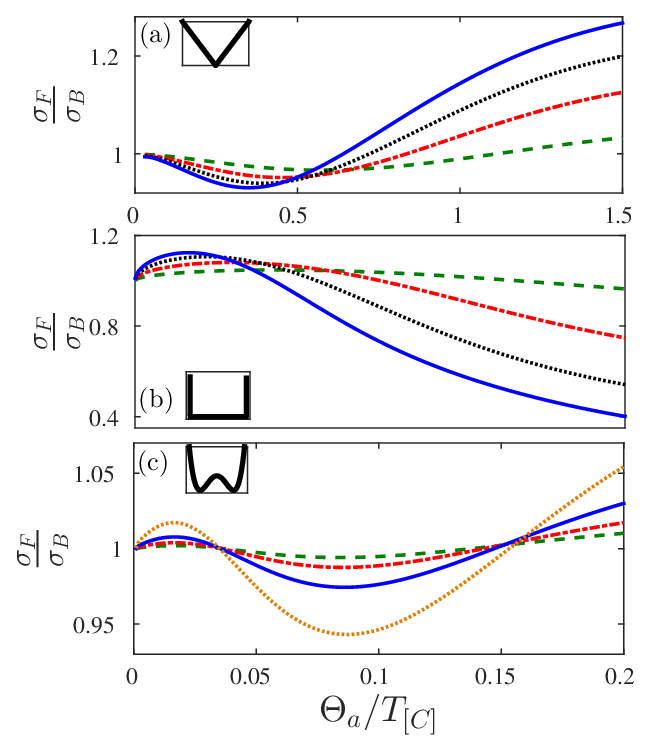
To gain deeper understanding we revert to Figs.4-5(a-b). The triangular and the square well potential have qualitatively opposite behaviors. When the highest temperature $T_{[C]}$ is small, the total entropy and the entropy change for the bosons in the triangular potential (respectively for the fermions in the square well potential) are much smaller than that of the fermions (respectively bosons), see Figs.2(c) and 3(c). It is easier to understand the qualitative behavior for large $T_{[C]}$ by considering the work exchanges. In this case the ratio of the work exchanges $\langle W_{[C]\rightarrow[D]}\rangle_{F}/\langle W_{[C]\rightarrow[D]}\rangle_{B}=\langle E_{[C]}\rangle_{F}/\langle E_{[C]}\rangle_{B}$ and thus it will eventually converge towards $1$ as the temperature increases. However the difference in the work processes $\langle W_{[C]\rightarrow[D]}\rangle_{F}-\langle W_{[C]\rightarrow[D]}\rangle_{B}$ behaves differently depending on the type of potential. It increases indefinitely for the square well, while it goes to $0$ for the triangular potential. Hence, for the square well potential the ratio $\langle W\rangle_{F}/\langle W\rangle_{B}$ will tend to $1$ from above, while for the triangular potential it will tend to $1$ from below [33]. The same analysis also explains the qualitatively similar behavior of the variance of the work probability distribution, Fig.5. For this quantity, however, the crossings of the line $\sigma_{F}/\sigma_{B}=1$ occur at a different values of $T_{[C]}$.

The double well (Fig.1(c)), is a typical example of a system in which the energy level spacing does not vary monotonically. Hence, we will use this to study the interplay of geometry and particle statistics in the performance of the engine cycle. As shown earlier in section II, the double well potential can have a scaling property so long as $\gamma\equiv\hbar\omega_{4}^{4}/m\omega_{2}^{3}$ is a constant. For ease of analytical and numerical analysis, we will focus on this case. As shown in Fig.4(c) the fermionic to bosonic ratio of the work output $\langle W_{F}\rangle/\langle W_{B}\rangle$ has a pronounced oscillatory behavior compared to potentials with monotonically changing energy level structure as the (inverse) temperature of the hot reservoir $\beta_{h}$.

The same behavior is expected and observed also for the ratio of the standard deviation of the work done for a fermionic over a bosonic working fluid $\sigma_{F}/\sigma_{B}$, see Fig.5(c).

References

- [1] M. Campisi, P. Hänggi, P. Talkner, Rev. Mod. Phys. 83, 771 (2011).
- [2] U. Seifert, Rep. Prog. Phys. 75, 126001 (2012).
- [3] R. Kosloff, Entropy 15, 2100 (2013).
- [4] G. Benenti, G. Casati, T. Prosen, K. Saito, arXiv:1311.4430 (2013).
- [5] D. Gelbwaser-Klimovsky, W. Niedenzu, G. Kurizki, arXiv:1503.01195 (2015).
- [6] P. Hänggi, P. Talkner, Nature Physics 11, 108 (2015).
- [7] M. Demirplak, S.A. Rice, J. Chem. Phys. B 109, 6838 (2005).
- [8] M. V. Berry, J. Phys. A: Math. Gen. 42 365303 (2009).
- [9] J. W. Deng, Q.-H. Wang, Z. H. Liu, P. Hänggi, J. B. Gong, Phys. Rev. E 88, 062122 (2013).
- [10] M. Palmero, E. Torrontegui, D. Gu�ry-Odelin, J. G. Muga, Phys. Rev. A 88 053423 (2013).
- [11] E. Torrontegui, S. Ibáez, S. Martínez-Garaot, M. Modugno, A. del Campo, D. Gu�ry-Odelin, A. Ruschhaupt, X. Chen, J. G. Muga, Adv. At. Mol. Opt. Phys. 62, 117 (2013).
- [12] S. Campbell, G. De Chiara, M. Paternostro, G.M. Palma, R. Fazio, arXiv:1410.1555 (2014).
- [13] S. Deffner, C. Jarzynski, A. del Campo, Phys. Rev. X 4, 021013 (2014).
- [14] A. del Campo, J. Goold, M. Paternostro, Sci. Rep.4, 6208 (2014).
- [15] J. R. Gomez-Solano, C. July., J. Mehl, C. Bechinger, http://arxiv.org/abs/1501.02568 (2015).
- [16] V. Blickle, T. Speck, L. Helden, U. Seifert, C. Bechinger, Phys. Rev. Lett. 96, 070603 (2006).
- [17] V. Blicke C. Bechinger, Nature Physics 8, 143 (2012).
- [18] S. An, J.-N. Zhang, M. Um, D. Lv, Y. Lu, J. Zhang, Z.-Q. Yin, H.T. Quan, K. Kim, Nature Physics 11, 193 (2015).
- [19] O. Abah, J. Roßnagel, G. Jacob, S. Deffner, F. Schmidt-Kaler, K. Singer, E. Lutz, Phys. Rev. Lett., 109, 203006 (2012).
- [20] M. Campisi, J. Pekola, R. Fazio, New J. Phys. 17, 035012 (2015).
- [21] Z. Gong, S. Deffner, H. T. Quan, Phys. Rev. E 90, 062121 (2014).
- [22] H. T. Quan, Y.-X. Liu, C. P. Sun, F. Nori, Phys. Rev. E 76, 031105 (2007).
- [23] Y. Zheng, D. Poletti, Phys. Rev. E 90, 012145 (2014).
- [24] A strong coupling significantly complicates the distinction between heat and work transferred to the system.
- [25] C. Jarzynski, Phys. Rev. A 88, 040101 (2013).
- [26] P. Talkner, E. Lutz, P. Hänggi, Phys. Rev. E. 75 050102 (2007).
- [27] The use of the grand-canonical partition function would not give accurate results in the regimes of particle numbers and temperatures we study. Moreover the canonical partition function allows us easy access to energy fluctuations for fixed particle number.
- [28] M. Wilkens, C. Weiss, J. Mod. Opt. 44, 1801 (1997).
- [29] C. Weiss, M. Wilkens, Opt. Express 1, 272 (1997).
- [30] V. Kashcheyevs arxiv:1110.6264 (2011).
- [31] Note that for the Harmonic oscillator and approach the same value in the high temperature limit.
- [32] If was too high, the difference between the fermionic and bosonic statistics will be much reduced.
- [33] In this case it plays particular importance the fact that at cold temperatures the work done in the cold arm is, in modulus, larger for the fermions than for the bosons. Hence, while the difference in work becomes negligible in one process, in the other process there is more work exchange for the fermions. The combination of these two effects results in a net work which is lower for the fermions.
Appendix A Derivation of recursive relation for the canonical partition function
Here, we derive Eq.(16) following the argument as presented in [30]. To do so we start from the grand canonical partition function , where or , is the subscript that denotes bosonic and fermionic statistics respectively. The grand partition function can be written as