Learning about probabilistic inference and forecasting
by playing with multivariate normal distributions
(with examples in R)
Abstract
The properties of the normal distribution under linear transformation, as well the easy way to compute the covariance matrix of marginals and conditionals, offer a unique opportunity to get an insight about several aspects of uncertainties in measurements. The way to build the overall covariance matrix in a few, but conceptually relevant cases is illustrated: several observations made with (possibly) different instruments measuring the same quantity; effect of systematics (although limited to offset, in order to stick to linear models) on the determination of the ‘true value’, as well in the prediction of future observations; correlations which arise when different quantities are measured with the same instrument affected by an offset uncertainty; inferences and predictions based on averages; inference about constrained values; fits under some assumptions (linear models with known standard deviations). Many numerical examples are provided, exploiting the ability of the R language to handle large matrices and to produce high quality plots. Some of the results are framed in the general problem of ‘propagation of evidence’, crucial in analyzing graphical models of knowledge.
“So far as the theories of mathematics are about reality,
they are not certain;
so far as they are certain, they are not about reality.
(A. Einstein)
“If we were not ignorant there would be no probability,
there could only be certainty.
But our ignorance cannot be absolute,
for then there would be no longer any probability at all.”
(H. Poincaré)
“Probability is good sense reduced to a calculus”
(S. Laplace)
“All models are wrong but some are useful”
(G. Box)
1 Introduction
The opening quotes set up the frame in which this paper has been written: in the sciences we always deal with uncertainties; being in condition on uncertainty we can only state ‘somehow’ how much we believe something; in order to do that we need to build up probabilistic models based on good sense. For example, if we are uncertain about the value we are going to read on an instrument, we can make probabilistic assessments about it. But in general our interest is the numerical value of a physics quantity. We are usually in great condition of uncertainty before the measurement, but we still remain with some degree of uncertainty after the measurement has been performed. Models enter in the construction of the the causal network which connects physics quantities to what we can observe on the instruments. They are also important because it is convenient to use, whenever it is possible, probability distributions, instead than to assign individual probabilities to each individual ‘value’ (after suitable discretization) that a physics quantity might assume.
As we know, there are good reasons why in many cases the Gaussian distribution (or normal distribution) offers a reasonable and convenient description of the probability that the quantity of interest lies within some bounds. But it is important to remember that, as it was clear to Gauss [1] when he derived the famous distribution for the measurement errors, one should not take literally the fact that the variable appearing in the formula can range from minus infinite to plus infinite: an apple cannot have infinite mass, or a negative one!
Sticking hereafter to Gaussian distributions, it is clear that if we are only interested to the probability density function (pdf) of a variable at the time, we can only describe our uncertainty about that quantity, and nothing more. The game becomes interesting when we study the joint distribution of several variables, because this is the way we can learn about some of them assuming the values of the others. For example, if we assume the joint pdf of variables and under the state of information (on which we ground our assumptions), we can evaluate , that is the pdf adding the extra condition , which is usually not the same as , that is the pdf of for any value might assume.11 1 The pdf is called marginal, although there is never special about this name, since all distributions of a single variable can be thought as being ‘marginal’ to all other possible quantities which we are not interested about. is instead ‘called’ conditional, although it is a matter of fact that all distributions are conditional to a given state of information, here indicated by . Note that throughout this paper will shall use the same symbol for all pdf’s, as it is customary among physicists – I have met mathematics oriented guys getting mad by the equation because, they say, “the three functions cannot be the same”…
Let us take for example the three diagrams of Fig. 1


to which we give a physical interpretation:
- 1.
In the diagram on the left the variable might represent the numerical value of a physics quantity, on which we are in condition on uncertainty, modelled by
(1) where and are suitable parameters to state our ‘ignorance’ about (‘complete ignorance’, if it does ever exist, is recovered in the limit ). Instead, is then what we read on an instrument when we apply it to . That is, even if we knew , we are still uncertain about what we can read on the instrument, as it is well understood. Modelling this uncertainty by a normal distribution we have, for any value of
(2) where is a compact symbol for and which is in general different from . In fact our uncertainty about (for any possible value of ) must be larger than that about itself, for obvious reasons – we shall see later the details.
- 2.
In the diagram on the center might represent a second observation done independently applying in general a second (possibly different) instrument to the identical value . This means that and are independent, although and are not, as we shall see.
- 3.
In the diagram on the right is the observation read on the instrument applies to , but possibly influenced by , that might then represent a kind of systematics.
Note, how it has been precisely stated, that of the first and of the second diagrams, as well as of the other two, are the readings on the instruments and not the result of the measurement! This is because by “result of the measurement” we mean statements about the quantity of interest and not about the quantities read on the instruments (think for example at the an experiment measuring the Higgs boson mass, making use of the information recorded by the detector!). In this case the “result of the measurement” would be where data stands for the set of observed variables.
The diagrams of the figure can be complicated, using sets of data, with systematics effects common to observations in each subset. The aim of this paper is to help in developing some intuition of what is going on in problems of this kind, with the only simplification that all pdf’s of interest are normal.
2 Technical premises (with some exercises)
We assume that the reader is familiar with some basic concepts related to uncertain numbers and uncertain vectors, usually met under the name of “random variables”.
2.1 Normal (Gaussian) distribution
:
| (3) |
with
| (4) | |||||
| (5) | |||||
| (6) |
(We remind that in most physics applications simply means .)
In the R language [2] there are functions
(dnorm(), pnorm() and qnorm(), respectively)
to calculate the pdf,
the cumulative function, usually indicated with
“’’, as well as its inverse, as shown
in the following, self explaining examples22
2
For information about
the language see one of the many tutorial available on the web.
Most functions we shall use here have self explaining names.
For an help, for example about dnorm(), just enter
> ?dnorm
(‘’ is the R console prompt):
> dnorm(0, 0, 1)
[1] 0.3989423
> 1/sqrt(2*pi) # (just a check)
[1] 0.3989423
> pnorm(0, 0, 1)
[1] 0.5
> pnorm(7, 5, 2) - pnorm(3, 5, 2)
[1] 0.6826895
> qnorm(0.5, 5, 2)
[1] 5
> qnorm(1, 5, 2)
[1] Inf
> qnorm(0, 5, 2)
[1] -Inf
Note the capability of the language to handle infinities,
as it can be cross checked by
> pnorm(Inf, 5, 2)
[1] 1
And here are the instructions to produce the plots of
figure 2.

mu <- 5; sigma <- 2; x <- seq(mu-5*sigma, mu+5*sigma, len=101)
plot(x, dnorm(x, mu, sigma), ty=’l’, ylab=’f(x)’, col=’blue’)
points(x, dnorm(x, mu, sigma*1.5), ty=’l’, lty=2, col=’blue’)
points(x, dnorm(x, mu, sigma*2), ty=’l’, lty=3, col=’blue’)
plot(x, pnorm(x, mu, sigma), ty=’l’, ylab=’F(x)’, col=’red’)
points(x, pnorm(x, mu, sigma*1.5), ty=’l’, lty=2, col=’red’)
points(x, pnorm(x, mu, sigma*2), ty=’l’, lty=3, col=’red’)
2.2 Bivariate and multivariate normal distribution
The joint distribution of a bivariate normal distribution is given by
| (7) | |||||
where
| (8) | |||||
| (9) | |||||
| (10) | |||||
| (11) | |||||
| (12) | |||||
| (13) |
with variances and covariances forming the covariance matrix
The bivariate pdf (7) can be rewritten in a compact form as
| (21) |
where stands for det(). This expression is valid for any number of variables and it turns, in the case is diagonal, into
| (22) |
(For an extensive, although mathematically oriented treatise on multivariate distribution see Ref. [3], freely available online.)
2.2.1 Multivariate normals in R
Functions to calculate multivariate normal pdf’s,
as well as cumulative functions and random generators
are provided in R via the package
mnormt33
3
http://cran.r-project.org/web/packages/mnormt/
that needs first to be installed44
4
For all technical details
about R (open source and multi-platform!) see
the R web site [2].
issuing
> install.packages("mnormt")
and then loaded
by the command
> library(mnormt)
Then we have to define the values of the parameters
and built up the vector of the central values and
the covariance matrix. Here is an example:
> m1=0.4; m2=2; s1=1; s2=0.5; rho=0.6
> mu <- c(m1, m2)
> ( V <- rbind( c( s1ˆ2, rho*s1*s2), c(rho*s1*s2, s2ˆ2) ) )
[,1] [,2]
[1,] 1.0 0.30
[2,] 0.3 0.25
Then we can evaluate the joint pdf in a point , e.g.
> dmnorm(c(0.5, 1.5), mu, V)
[1] 0.1645734
Or we can evaluate , or
, respectively, with
> pmnorm(c(0.5, 1.5), mu, V)
[1] 0.140636
and
> pmnorm(mu, mu, V)
[1] 0.3524164
2.3 Graphical representation of normal bivariates
If we like to visualize the
joint distribution we need a 3D graphical package, for example
rgl55
5
https://r-forge.r-project.org/projects/rgl/
or plot3D.66
6
http://www.r-bloggers.com/3d-plots-in-r/
We need to evaluate the joint pdf on a grid
of values ‘’ and ‘’ and provide them to the suited function.
Here are the instructions that use the persp3d() of the
rgl package:
> library(rgl)
> fun <- function(x1,x2) dmnorm(cbind(x1, x2), mu, V)
> x1 <- seq(m1-3*s1, m1+3*s1, len=51)
> x2 <- seq(m2-3*s2, m2+3*s2, len=51)
> f <- outer(x1, x2, fun)
> persp3d(x1, x2, f, col=’cyan’, xlab="x1", ylab="x2", zlab="f(x1,y2)")
After the plot is shown in the graphics window, the window can be enlarged
and the plot rotated at wish. Figure 3
shows in the upper two plots two views of the
same distribution.


Here are also the instructions to use plot3D():
> library(plot3D)
> M <- mesh(x1, x2)
> surf3D(M$x, M$y, f, bty=’b2’, phi = 30, theta = -20,
+ xlab=’x1’, ylab=’x2’, zlab=’f(x1,x2)’)
The result is shown in the lower
plot of Fig. 3.
Another convenient and often used representation of normal bivariates is to draw iso-pdf contours, i.e. lines in correspondence of the points in the plane such as . This requires that the quadratic form at the exponent of Eq. (7) [that is what is written in general as ] has a fixed value. In the two dimensional case of Eq. (7) we recognize the expression of an ellipse. We have in R the convenient package ellipse77 7 http://cran.r-project.org/web/packages/ellipse/ to evaluate the points of such an ellipse, given the vector of expected values, the covariance matrix and the probability that a point falls inside it. Here is the script that applies the function to the same bivariate normal of Fig. 3, thus producing the contour plots of Fig. 4:

plot( ellipse(V, centre=mu, level=0.9973), ty=’l’, lty=2, col=’red’,
     asp=1, xlab=expression(x[1]), ylab=expression(x[2]) )
points( ellipse(V, centre=mu, level=0.99), ty=’l’, col=’blue’)
points( ellipse(V, centre=mu, level=0.954), ty=’l’, lty=2, col=’red’)
points( ellipse(V, centre=mu, level=0.5), ty=’l’, col=’blue’)
points( ellipse(V, centre=mu, level=0.683), ty=’l’,  lty=2, col=’red’)
points( ellipse(V, centre=mu, level=0.90), ty=’l’, col=’blue’)
points(mu[1], mu[2], pch=3, cex=1.5, col=’blue’)
for(k in 1:3) {
  abline(v=mu[1]-k*sqrt(V[1,1]), lty=3, col=’magenta’)
  abline(v=mu[1]+k*sqrt(V[1,1]), lty=3, col=’magenta’)
  abline(h=mu[2]-k*sqrt(V[2,2]), lty=3, col=’magenta’)
  abline(h=mu[2]+k*sqrt(V[2,2]), lty=3, col=’magenta’)
}
The probability to find a point inside the ellipse contour is defined by the argument level. The ellipses drawn with solid lines define, in order of size, 50%, 90% and 99% contours. For comparison there are also the contours at 68.3%, 95.5% and 99.73%, which define the highly confusing 1- , 2- and 3- contours. Indeed, the probability that each of the variable falls in the interval of has little to do with these ellipses. If we are interested to the probability that a point falls in a rectangles defined by the probability needs to be calculated making the integral of the joint distribution inside the rectangle (some of these rectangles are shown in Fig. 4 by the dotted lines, that indicate 1- , 2- and 3- bound in the individual variable).
Let us see how to evaluate in R the probability that a point
falls in a rectangle, making use of the cumulative probability
function pmnorm(). In fact the probability in a rectangle
is related to the cumulative distribution by the following relation
| (23) | |||||
that can be implemented in an R function:
p.rect.norm <- function(xlim, ylim, mu, V, sigmas=FALSE, ...) {
  # The argument ’...’ might be useful to pass extra arguments to pmnorm.
  if ( (length(mu) != 2) | sum( dim(V) != c(2,2) )   # some check
      | (length(xlim) != 2) | (length(ylim) != 2) ) {
    print("wrong dimensions in one of parameters")
    return(NULL)
  } else if ( sum( eigen(V)$values <= 0 ) >  0) {
    cat( sprintf("V is not positively defined\n") )
    return(NULL)
  }
  # If argument ’sigmas’ is TRUE:
  if( sigmas ) { # rectangular defined in units of individual sigma around mu
    xlim <- mu[1] + xlim * sqrt(V[1,1])
    ylim <- mu[2] + ylim * sqrt(V[2,2])
  }
  library(mnormt)
  p.rect <- pmnorm( c(xlim[2], ylim[2]), mu, V, ...) -
            pmnorm( c(xlim[2], ylim[1]), mu, V, ...) -
            pmnorm( c(xlim[1], ylim[2]), mu, V, ...) +
            pmnorm( c(xlim[1], ylim[1]), mu, V, ...)
  return(p.rect)
}
For example88
8
For Monte Carlo oriented guys, here is how to
cross check the results (don’t expect to reproduce 51313!):
> xy <- rmnorm(100000, mu, V)
> length( xy[,1][ xy[,1] > m1 - s1 & xy[,1] < m1+s1 & xy[,2] > m2 - s2 & xy[,2] < m2+s2 ] )
[1] 51313
> p.rect.norm(c(m1-s1, m1+s1), c(m2-s2, m2+s2), mu, V)
[1] 0.5138685
> p.rect.norm(c(-1, 1), c(-1, 1), mu, V, sigmas=TRUE)
[1] 0.5138685
As a cross check, let us calculate the probabilities in strips
of plus/minus one standard deviations around the
averages (the ‘strips’ provide a good intuition of what
a ‘marginal’ is):
> p.rect.norm(c(-1, 1), c(-10, 10), mu, V, sigmas=TRUE)
[1] 0.6826895
> p.rect.norm(c(-10, 10), c(-1, 1), mu, V, sigmas=TRUE)
[1] 0.6826895
2.4 Marginals (and ‘multivariate marginals’) of multivariate normals
A nice feature of the multivariate normal distribution is that if we are just interested to a subset of variables alone, neglecting which value the other ones can take (‘marginalizing’), we just drop from and from the uninteresting values, or the relative rows and columns, respectively. For example, if we have – see subsection 6.1.2 –
| (24) |
marginalizing over the second variable (i.e. being only interested in the first and the third) we obtain
| (25) |
Here is a function that returns expected values and variance of the multivariate ‘marginal’
marginal.norm <- function(mu, V, x.m) {
  # x.m is a vector with logical values (or non zero) indicating
  # the elements on which to marginalise (the others are 0, NA or FALSE)
  x.m[is.na(xm)] <- FALSE
  v <- which( as.logical(x.m) )
  list(mu=mu[v], V=V[v, v])
}
(Note how the function has been written in a very compact form, exploiting some peculiarities of the R language. In particular, the elements of x.m to which we are interested can be TRUE, or can be a numeric value different from zero; the others can be FALSE, 0 or NA.)
2.5 Conditional distribution of a variable, given its bivariate distribution with another variable
A different problem is the pdf of one of variables, say , for a given value of the other. This is not as straightforward as the marginal (and for this reason in this subsection we only consider the bivariate case). Fortunately the distribution is still a Gaussian, with shifted central value and squeezed width:
| (26) |
i.e.
| (27) | |||||
| (28) | |||||
| (29) |
And, by symmetry,
| (30) |
Mnemonic rules to remember Eqs. (27) and (28) are
- •
the shift of the expected value depends linearly on the correlation coefficient as well on the difference between the value of the conditionand () and its expected value (); the ratio can be seen as a minimal dimensional factor in order to get a quantity that has the same dimensions of (remember that and have in general different physical dimensions);
- •
the variance is reduced by a factor which depends on the absolute value of the correlation coefficient, but not on its sign. In particular it goes to zero if , limit in which the two quantities become linear dependent, while it does not change if , since the two variables become independent and they cannot effect each other. (In general independence implies . For the normal bivariate it is also true the other way around.)

An example of a bivariate distribution (from [5], with and indicated as customary with and ) is given in Fig. 5, which shows also the marginals and some conditionals.
2.5.1 Evaluation of a conditional from a given bivariate normal
As an exercise, lets prove (26), with the purpose of show some useful tricks to simplify the calculations. If we take literally the rule to evaluate knowing that is given by (7) we need to calculate
| (31) |
The trick is to make the calculations neglecting all irrelevant multiplicative factors, starting from the whole denominator , which is a number given (whatever its value might be!).
Here are the details (note that additive terms in the exponential are factors in the function of interest!):99 9 Essentially the trick consists in observing that if we have a pdf proportional to , then it is also proportional to that is a Gaussian with and .
| (32) | |||||
in which we recognize a Gaussian with expected value and standard deviation (and therefore the normalization factor can be obtained without any calculation).
2.6 Linear combinations
Linear transformations of variables are important because there are several practical problems to which they apply. There are also other cases in which the transformation is not rigorously linear, but it can be still approximately linearized in the region of interest, where the probability mass is concentrated. There are well known theorems that relate expected values and covariance matrix of the input quantities to expected values and covariance matrix of the output quantities. The most famous case is when a single output quantity depends on several variables . So, given
| (33) |
there is a relation which always holds, no matter if the are independent or not and whichever are the pdf’s which describe them:
| (34) |
In the special case that the are also independent, we have
| (35) |
Instead it is not always simple to calculate the pdf of in the most general case. There are however two remarkable cases, which we assume known and just recall them here, in which is is normally distributed:
- 1.
linear combinations of normally distributed variables are still normal;
- 2.
the Central Limit Theorem states that if we have ‘many’1010 10 The theorem says “for that goes to infinity”! Some practice is then needed to judge when it is large enough – often around 10 is can be considered ‘large’, in other cases even is not enough! (Think of one million of variables described by a Poisson distribution with .) independent variables their linear combination is normally distributed with variance equal to if none of the non-normal components dominates the overall variance, i.e. if , where denotes any of those non-normal components.
Since in this paper we only stick to normal pdf’s, the only task will be to evaluate the covariance matrix of the set of variables of interest, depending on the problem.
The general transformation from input variables to output variable is given by1111 11 We neglect a possible extra constant term in the linear combination because this plays no role in the uncertainty.
| (36) |
or, in a compact form that use the transformation matrix , whose elements are the ,
| (37) |
Expected value and covariance matrix of the output quantities are given by
| (38) | |||||
| (39) |
For example, if , with , and , and the transformation rule is given by
| (40) | |||||
| (41) |
i.e.
we get in R: 1212
12
The function outer() produces
by default a matrix which is by default is the outer
product of two vectors, i.e. . But
it has a third parameter FUN which which it is possible
to evaluate different function on the ‘grid’ defined by
the Cartesian product of the two vector. Try for example
> outer(1:3, 1:3, ’+’)
> outer(1:3, 1:3, function(x,y) x + yˆ2))
> round( outer(0:10, 0:10, function(x,y) sin(x)*cos(y)), 2 )
> mu.X <- c(2, -3)
> s.X <- c(0.2, 0.5)
> rho.X   <- -0.8
> V.X  <- outer(s.X, s.X)
> V.X[1,2] <- V.X[2,1] <- V.X[1,2]*rho.X
> V.X
      [,1]  [,2]
[1,]  0.04 -0.08
[2,] -0.08  0.25
> ( cor.X <- V.X / outer(s.X,s.X) )
     [,1] [,2]
[1,]  1.0 -0.8
[2,] -0.8  1.0
> ( C <- rbind( c(1,2), c(-1,1) ) )
     [,1] [,2]
[1,]    1    2
[2,]   -1    1
> ( mu.Y <- as.vector( C %*% mu.X ) )
[1] -4 -5
> ( V.Y <- C %*% V.X %*% t(C) )
     [,1] [,2]
[1,] 0.72 0.54
[2,] 0.54 0.45
> ( s.Y   <- sqrt(diag(V.Y)) )
[1] 0.8485281 0.6708204
> ( cor.Y <- V.Y / outer(s.Y,s.Y) )
          [,1]      [,2]
[1,] 1.0000000 0.9486833
[2,] 0.9486833 1.0000000
Let us get a visual representation of the probability distribution of and using this time, instead of iso-pdf ellipses, points in the plane produced by the random generator provided by the package mnormt (see result in Fig. 6):
> n=5000; r.X <- rmnorm(n, mu.X, V.X); r.Y <- rmnorm(n, mu.Y, V.Y)
> plot(r.X, col=’magenta’, xlim=c(-7,2), ylim=c(-8,-1), cex=0.2,
+  asp=1, xlab=’X1 ,  Y1’,  ylab=’X2 , Y2’)
> points(r.Y, col=’cyan’, cex=0.2)

2.7 Conditional distributions in many dimensions
Instead, a less known rule is that which gives the covariance matrix of a conditional distribution with a number of variables above two. For example we might have 5 variables and could be interested in the expected values and the covariance matrix of , given . Problems of this kind might look a mere mathematical curiosity, but they are indeed important to understand how we learn from data and we make probabilistic predictions using probability theory.
Compact formulae to solve this problems can be found in Ref. [3]. If we partition and into the the subsets of variable on which we want to condition and the other ones, i.e.
the result is
| (51) | |||||
| (52) |
(And analogous formulae for and .)
In the case of a bivariate distributions we recover easily Eqs. (27)-(28), as it follows.
- Expected value:
-
is the off-diagonal term , while is equal to . Eq. (51) becomes then
(53) - Variance:
-
The remaining two terms of interest are also very simple: is , while , equal to , is . It follows
(54)
Note that, while the conditioned expected value depends on the conditionand vector , the conditioned variance does not.
3 R implementation of the rule to condition multivariate normal distributions
At this point, having set up all our tools, here is the R function which implements the above formulae:1313 13 As it will be mentioned in the footnote 23 of Sec. 10, a more numerically stable way to invert a matrix in R would be using the Choleski decomposition, but for the purpose of this note the difference is slightly appreciable.
norm.mult.cond <- function(mu, V, x.c, full=TRUE) {
  out <- NULL
  n <- length(mu)

  # Checks dimensions of mu and V
  if ( sum(dim(V) != n) ) {
    cat( sprintf("dimensions of V incompatible with length of mu\n") )
    return(out)
  }

  # number of conditionand variables
  nc <- length(x.c[!is.na(x.c)])
  # peculiar/anomalous cases
  if( (length(x.c) > n) | (nc > n) ) {
    cat( sprintf("x.c has more elements than mu\n") )
    return(out)
  } else if (nc == 0) {  # No condition
    out$mu <- mu
    out$V  <- V
    return(out)
  } else if(nc == n) {
    out$mu <- x.c    # exact values
    out$V  <- NULL   # covariance matrix is meaningless
    return(out)
  }

  # Apply Eaton’s formulae
  v.c <- which(!is.na(x.c))  # conditioning variables
  v   <- which(is.na(x.c))   # variables of interest
  V11 <- V[v, v]
  V22 <- V[v.c, v.c]
  V12 <- V[v, v.c]
  V21 <- V[v.c, v]
  mu.cond <- mu[v] + V12 %*% solve(V22) %*%  (x.c[!is.na(x.c)] - mu[v.c])
  V.cond  <- V11 - V12 %*% solve(V22) %*% V21
  if(!full) { # returns only interesting part
    out$mu <- as.vector(mu.cond)
    out$V  <- V.cond
  } else {    # returns all (better to understand!!)
    mu1 <- mu
    V1 <- V
    mu1[v]   <- mu.cond
    mu1[v.c] <- x.c[!is.na(x.c)]
    V1[v, v] <- V.cond
    V1[v.c, v.c] <- 0
    V1[v, v.c]   <- 0
    V1[v.c, v]   <- 0
    out$mu <- as.vector(mu1)
    out$V  <- V1
  }
  return(out)
}
The conditionand vector x.c has to contain numbers in the positions corresponding to the variables on which we want to condition, and NA, that is ‘not available’ or ‘unknown’, in the others, as we shall see in the examples. The code of parameter full is to return the vector of expectation and the covariance having the initial dimensionality. The expectation of the variable used as condition is the condition itself. All elements of the covariance matrix related to conditionals are instead zero, and the utility of this convention will be clear going through the examples.
Let us try with a simple case of two normal quantities of section 2.6. The question is how our uncertainty on change if we assume :
> ( V.X.cond <- norm.mult.cond(mu.X, V.X, c(NA, -2)) )
$mu
[1]  1.68 -2.00

$V
       [,1] [,2]
[1,] 0.0144    0
[2,] 0.0000    0

> sqrt(diag(V.X.cond$V))
[1] 0.12 0.00
The effect of the conditions to shift the expected value of from 2 to 1.68 and to squeeze its standard uncertainty to 0.12. If we provide our result in the conventional form “expected value standard uncertainty”, the assumption (or ‘knowledge’) updates our ‘knowledge’ about from ‘’ to ‘’.
4 The ‘simplest experiment’
Let us go back to the first diagram of Fig. 1, that we repeat here for convenience:
This diagram describes the situation in which we have the physical quantity , that is a parameter of our physical model of reality, and the reading on an instrument, , caused by .
The instrument has been well calibrate, such to give around , but it is not perfect, as usual. In other words, even if we knew exactly the value we were not sure about the value we would read. For simplicity, let us model this uncertainty by a normal distribution, i.e.
| (55) |
But we usually do not know , and therefore we are even more uncertain about what we shall read on the instrument. In fact we are dealing with a joint distribution describing the joint uncertainty about the two quantities, that is
| (56) |
Our knowledge about will be given, instead, by , a distribution characterized by .
It is convenient to model our uncertainty about with a normal distribution, with a standard deviation much larger than -- if we make a measurement we want to gain knowledge about that quantity! -- and centered around the values we roughly expect.1414 14 For extensive discussions about modelling prior knowledge of physical quantities see Ref. [5] and references therein. As a practical example, think at the width of the table at which a sit in the very moment you read these lines (or any other object), and about the reading on a ruler when you try to measure it.
In order to simplify the calculations, in the exercise that follows let us assume that is centered around zero. We shall see later how to get rid of this limitation.
The joint distribution is then given by
| (57) |
As an exercise, let us see how to evaluate . The trick, already applied before, is to manipulate the terms in the exponent in order to recover a well known pattern. Here are the details, starting from (57) rewritten dropping all irrelevant factors:
| (58) | |||||
| (59) | |||||
| (60) | |||||
| (61) | |||||
| (62) | |||||
| (63) |
In this expression we recognize a bivariate distribution centered around , provided we interpret
| (64) | |||||
| (65) |
and after having checked the consistency of the terms multiplying . Indeed we have
| (66) | |||||
| (67) |
and then the second term within parenthesis can be rewritten as
| (68) |
Then
| (69) |
is definitively a bivariate normal distribution with
As a cross check, let us evaluate expected value and variance of if we assume a certain value of , for example :
| (76) | |||||
| (77) |
as it should be: provided we know the value of our expectation of is around its value, with standard uncertainty .
More interesting is the other way around, that is indeed the purpose of the experiment: how our knowledge about is modified by :
| (78) | |||||
| (79) |
Contrary to the first case, this second result is initially not very intuitive: the expected value of is not exactly equal to the ‘observed’ value , unless , that models our prior standard uncertainty about , is much larger than the experimental resolution . Similarly, the final standard uncertainty is in general a smaller than , unless, again, .1515 15 You might recognize in Eq. (79) which stems naturally from probability theory and tells how a new observation squeezes the uncertainty on the true value of a quantity. Indeed, it easy to show that Eq. 78 can be written, as rather well known (see e.g. Ref. [5]), as weighted average of the prior expected value and observation, with weights equal to the prior variance and the instrument variance. En passent we can rewrite Eqs. (78)-(79) as or with in order to emphasize the Kalman filter’s updating rules. [4] Although initially surprising, these result are in qualitative agreement with the good sense of experienced physicists [5].
5 Several independent measurements on the same physics quantity
The next step is to see what happens when we are in the conditions to make several independent measurements on the same quantity , possibly with different instruments, each one characterized by a conditional standard uncertainty and perfectly calibrated, that is . The situation can be illustrated with the diagram at the center of Fig. 1, reported here for convenience, extended to other observations:
![[Uncaptioned image]](1504.02065v1/x1-x2x3x4x5x6.png)
We have learned that if we are able to build up the covariance matrix of the joint distribution the problem is readily solved, at least in the normal approximations we are using throughout the paper.
In principle we should repeat the previous exercise to evaluate, sticking to the first two observations and ,
| (80) | |||||
| (81) |
where in the last step we have made explicit that does not depend on , once is known. But this does not implies that and are independent, as we shall see later! They are simply conditionally independent, i.e. independent under the condition (to be meant in general as an hypothesis) that has a precisely known value.
In reality we do not need to go through a similar derivation, that indeed was just an exercise. The easy solution arises, going back to the previous case, noting that the observation is the sum of the value of the physics quantity and the instrumental error (a ‘noise’, as you might like to see it), i.e.
| (82) |
with modelled, as usual, by a normal distribution, that is, in general
| (83) |
The general uncertain vector will be then , as clarified by the following diagram:
![[Uncaptioned image]](1504.02065v1/x1-x2x3x4x5x6_nomi.png)
These are then the first terms the transformation rules:
| (84) | |||||
| (85) | |||||
| (86) |
from which the calculation of the covariance matrix is straightforward:
- •
the -th element diagonal is given by the variance of , that is , , and so on;
- •
the off-diagonal elements are all equal to , because the only element in common in all linear combinations is .
Hence here is the covariance matrix of interest:
5.1 Getting some insights with numerical examples
At this point, instead of trying to get analytic formulae for all conditional probabilities of interest, we prefer to use the properties of the multivariate normal distribution implemented in the function norm.mult.cond() seen before. And, since the game is now automatic, we enlarge our space to 6 variables, for the ‘true value’ and - for four possible ‘readings’. Although it is not any longer needed, we still set out prior central value about around , which is equivalent to set to 0 all expected values. (For didactic purposes we have set only 10 larger than the experimental resolutions , as we shall discuss commenting the results.) Here is the R code, with some comments:
> n=6; muX1=0; sigmaX1=10                 # set size and initial uncertainty on X1
> mu <- rep(muX1, n)                      # set expected values (all equal!)
> ( sigma <- c(sigmaX1, rep(1,n-1)) )     # standard deviations
[1] 10  1  1  1  1  1
> V <- matrix(rep(sigma[1]^2, n*n), c(n,n))
> diag(V)[2:n] <- diag(V)[2:n] + sigma[2:n]^2
> V                                               # covariance matrix
     [,1] [,2] [,3] [,4] [,5] [,6]
[1,]  100  100  100  100  100  100
[2,]  100  101  100  100  100  100
[3,]  100  100  101  100  100  100
[4,]  100  100  100  101  100  100
[5,]  100  100  100  100  101  100
[6,]  100  100  100  100  100  101
> (su <- sqrt(diag(V)))                                 # standard deviations
[1] 10.00000 10.04988 10.04988 10.04988 10.04988 10.04988
> V/outer(su,su)                                        # correlation matrix
          [,1]      [,2]      [,3]      [,4]      [,5]      [,6]
[1,] 1.0000000 0.9950372 0.9950372 0.9950372 0.9950372 0.9950372
[2,] 0.9950372 1.0000000 0.9900990 0.9900990 0.9900990 0.9900990
[3,] 0.9950372 0.9900990 1.0000000 0.9900990 0.9900990 0.9900990
[4,] 0.9950372 0.9900990 0.9900990 1.0000000 0.9900990 0.9900990
[5,] 0.9950372 0.9900990 0.9900990 0.9900990 1.0000000 0.9900990
[6,] 0.9950372 0.9900990 0.9900990 0.9900990 0.9900990 1.0000000
As we can see, all variables are correlated! The reason is very simple: any precise information we get about one of them changes the pdf of all others. In physics terms, a reading on a instrument changes our opinion about the value of the quantity of interest as well as of all other readings we have not yet done (or we not yet aware of their values – in probability theory what matters is not time ordering, but ignorance).
Let us now see what happens if we condition on a precise value of the true value , for example :
> ( mu.c <- c(2, rep(NA, n-1)) )                    # conditionand
[1]  2 NA NA NA NA NA
> ( out<- norm.mult.cond(mu, V, mu.c) )             # resulting multivariate
$mu
[1] 2 2 2 2 2 2

$V
     [,1] [,2] [,3] [,4] [,5] [,6]
[1,]    0    0    0    0    0    0
[2,]    0    1    0    0    0    0
[3,]    0    0    1    0    0    0
[4,]    0    0    0    1    0    0
[5,]    0    0    0    0    1    0
[6,]    0    0    0    0    0    1
As we see, the expected values are all equal, is not longer uncertain, and all other variables become independent, more precisely “conditional independent”
Let’s now see what happens if we condition instead on the observation :
> ( mu.c <- c(NA, 2, rep(NA, n-2)) )
[1] NA  2 NA NA NA NA
> ( out<- norm.mult.cond(mu, V, mu.c) )
$mu
[1] 1.980198 2.000000 1.980198 1.980198 1.980198 1.980198

$V
         [,1] [,2]     [,3]     [,4]     [,5]     [,6]
[1,] 0.990099    0 0.990099 0.990099 0.990099 0.990099
[2,] 0.000000    0 0.000000 0.000000 0.000000 0.000000
[3,] 0.990099    0 1.990099 0.990099 0.990099 0.990099
[4,] 0.990099    0 0.990099 1.990099 0.990099 0.990099
[5,] 0.990099    0 0.990099 0.990099 1.990099 0.990099
[6,] 0.990099    0 0.990099 0.990099 0.990099 1.990099

> ( out.s <- sqrt(diag(out$V)) )                 # standard deviations
[1] 0.9950372 0.0000000 1.4107087 1.4107087 1.4107087 1.4107087
> out$V / outer(out.s, out.s)                    # correlation matrix (besides NaN)
          [,1] [,2]      [,3]      [,4]      [,5]      [,6]
[1,] 1.0000000  NaN 0.7053456 0.7053456 0.7053456 0.7053456
[2,]       NaN  NaN       NaN       NaN       NaN       NaN
[3,] 0.7053456  NaN 1.0000000 0.4975124 0.4975124 0.4975124
[4,] 0.7053456  NaN 0.4975124 1.0000000 0.4975124 0.4975124
[5,] 0.7053456  NaN 0.4975124 0.4975124 1.0000000 0.4975124
[6,] 0.7053456  NaN 0.4975124 0.4975124 0.4975124 1.0000000
The ‘measurement’ has had the effect of changing all our expectations, becoming all ‘practically equal’ to the observed value of . But the uncertainties about the possible ’future observations’ are different than that of the true value . They are in fact larger by a factor (see also Fig. 7). The reason is that and (i.e. and ) and all other possible readings , and ‘communicate’ each other via : their uncertainty is than the combination (quadratic combination!) of that assigned to and that of the readings if we new exactly (that is ).

Let us see if we add another observation, e.g. , that is we recondition now simultaneously on and
> mu.c <- c(NA, 2, 1, NA, NA, NA)
> ( out<- norm.mult.cond(mu, V, mu.c) )
$mu
[1] 1.492537 2.000000 1.000000 1.492537 1.492537 1.492537

$V
          [,1] [,2] [,3]      [,4]      [,5]      [,6]
[1,] 0.4975124    0    0 0.4975124 0.4975124 0.4975124
[2,] 0.0000000    0    0 0.0000000 0.0000000 0.0000000
[3,] 0.0000000    0    0 0.0000000 0.0000000 0.0000000
[4,] 0.4975124    0    0 1.4975124 0.4975124 0.4975124
[5,] 0.4975124    0    0 0.4975124 1.4975124 0.4975124
[6,] 0.4975124    0    0 0.4975124 0.4975124 1.4975124

> ( out.s <- sqrt(diag(out$V)) )
[1] 0.7053456 0.0000000 0.0000000 1.2237289 1.2237289 1.2237289

> out$V / outer(out.s, out.s)
          [,1] [,2] [,3]      [,4]      [,5]      [,6]
[1,] 1.0000000  NaN  NaN 0.5763904 0.5763904 0.5763904
[2,]       NaN  NaN  NaN       NaN       NaN       NaN
[3,]       NaN  NaN  NaN       NaN       NaN       NaN
[4,] 0.5763904  NaN  NaN 1.0000000 0.3322259 0.3322259
[5,] 0.5763904  NaN  NaN 0.3322259 1.0000000 0.3322259
[6,] 0.5763904  NaN  NaN 0.3322259 0.3322259 1.0000000
As we can see, after the second observation the expected values are practically equal to 1.5, average between the two readings. The uncertainty about the true value has decreased by a factor 1.41, that is , while the uncertainties about the forecasting decrease only by a factor 1.15, going from 1.41 to 1.22. This latter number can be understood as , as it will be justified in a while.
Let us see what happens if we suppose that also is precisely known, namely (different from previously used, not only “just to change” but also to use a value different from that of and ):
> mu.c <- c(3, 2, 1, NA, NA, NA)
> ( out<- norm.mult.cond(mu, V, mu.c) )
$mu
[1] 3 2 1 3 3 3

$V
     [,1] [,2] [,3]          [,4]          [,5]          [,6]
[1,]    0    0    0  0.000000e+00  0.000000e+00  0.000000e+00
[2,]    0    0    0  0.000000e+00  0.000000e+00  0.000000e+00
[3,]    0    0    0  0.000000e+00  0.000000e+00  0.000000e+00
[4,]    0    0    0  1.000000e+00 -2.302158e-12 -2.302158e-12
[5,]    0    0    0 -2.302158e-12  1.000000e+00 -2.302158e-12
[6,]    0    0    0 -2.302158e-12 -2.302158e-12  1.000000e+00
If is perfectly known the observations and are irrelevant, as it has to be.1616 16 And if and are ‘very far’ from ? In this simple model we are using, there is little to do, because any observation from minus infinite to plus infinite is never incompatible with a any Gaussian. But we know by experience that something strange might be happened. It this case we need to put in mathematical form the model we have in mind.
Finally, going back to the physical case of interest, in which is unknown, let us add a third observation, e.g.
> mu.c <- c(NA, 2, 1, 0, NA, NA)
> ( out<- norm.mult.cond(mu, V, mu.c) )
$mu
[1] 0.9966777 2.0000000 1.0000000 0.0000000 0.9966777 0.9966777

$V
          [,1] [,2] [,3] [,4]      [,5]      [,6]
[1,] 0.3322259    0    0    0 0.3322259 0.3322259
[2,] 0.0000000    0    0    0 0.0000000 0.0000000
[3,] 0.0000000    0    0    0 0.0000000 0.0000000
[4,] 0.0000000    0    0    0 0.0000000 0.0000000
[5,] 0.3322259    0    0    0 1.3322259 0.3322259
[6,] 0.3322259    0    0    0 0.3322259 1.3322259

> ( out.s <- sqrt(diag(out$V)) )
[1] 0.5763904 0.0000000 0.0000000 0.0000000 1.1542209 1.1542209
> out$V / outer(out.s, out.s)
          [,1] [,2] [,3] [,4]      [,5]      [,6]
[1,] 1.0000000  NaN  NaN  NaN 0.4993762 0.4993762
[2,]       NaN  NaN  NaN  NaN       NaN       NaN
[3,]       NaN  NaN  NaN  NaN       NaN       NaN
[4,]       NaN  NaN  NaN  NaN       NaN       NaN
[5,] 0.4993762  NaN  NaN  NaN 1.0000000 0.2493766
[6,] 0.4993762  NaN  NaN  NaN 0.2493766 1.0000000
As we can see, the value of is with very good approximation the average of the three observations, that is 1, with a the standard uncertainty decreasing with , passing from 1.00 to 0.71 to 0.58. This is because the three pieces of information enter with the same weight, since , related to the ‘precision of the instrument’, is the same in all cases and equal to 1.
As far as the prediction of future observations, obviously they must be centered around the value we believe is, at the best of our knowledge, a value which changes with the observations. As far as uncertainty and correlation coefficient are concerned, they decrease as follows (starting from the very beginning, before any observation):
- Standard uncertainty:
-
10.05, 1.41, 1.22, 1.15.
We can see that they are a quadratic combination of the uncertainty with which we know and that with which we expect the observation given a precise value of . If we indicate the state of information at time as , the rule is(91) Asymptotically, when after many measurements the determination of is very accurate, it only remains , as it has to be.
- Correlation coefficient:
-
0.990, 0.50, 0.33, 0.25.
It is initially very high because any new observation changes dramatically our expectation about the others. But then, when we have already made several observations, a new one has only very little effect on our forecasting. Asymptotically, when we have made a very large number of observations and is very well ‘determined’, all future observations become essentially “conditionally independent”.
5.2 Follows up
At this point the game can be continued with different options. One has only to re-build the initial covariance matrix and play changing the conditions.
An interesting exercise is certainly that of increasing , for example to 100, i.e. 100 times large than the ‘precision’ of our instrument, or even 1000, to see how our conclusions change. The result will be that true value and future measurements are ‘practically’ only determined by the observations.
It could also interesting to see what happens if the different observations come from instruments having different precisions.
Finally, one could produce a (relatively) large random sample of observations measuring the same true value. Being the number of observations, the dimensionality of our problem will be , because we have to add – obviously – and we want to have at least two future observations ( and ) in order to check their degree of correlation. Here is the R session in which we have been playing with a sample of 100 observations (for obvious reasons we shall focus only on the uncertain variables, i.e. , and ):
> m <- 100; n <- m + 3  # dimensionality of the problem
> mu <- rep(0,n)
> sigma <- c(10, rep(1,n-1))
> V <- matrix(rep(sigma[1]^2, n*n), c(n,n))
> diag(V)[2:n] <- diag(V)[2:n] + sigma[2:n]^2
> ( X1.God <- 2 )  # the exact value of the quantity we are going to measure
[1] 2
> sample <- rnorm(m, X1.God, sigma[2])   # random sample
> mean(sample)                           # sample mean
[1] 2.094649
> mu.c <- c(NA, sample, NA, NA)
> out <- norm.mult.cond(mu, V, mu.c)     # no printouts, for obvious reasons
> ( out <- marginal.norm(out$mu, out$V, c(1, rep(0, m), 1, 1)) ) # interesting part
$mu
[1] 2.094439 2.094439 2.094439

$V
         [,1]     [,2]     [,3]
[1,] 0.009999 0.009999 0.009999
[2,] 0.009999 1.009999 0.009999
[3,] 0.009999 0.009999 1.009999

> ( su <- sqrt(diag(out$V)) )
[1] 0.099995 1.004987 1.004987

> out$V /outer(su,su)
           [,1]       [,2]       [,3]
[1,] 1.00000000 0.09949879 0.09949879
[2,] 0.09949879 1.00000000 0.00990001
[3,] 0.09949879 0.00990001 1.00000000
Expected values of the true value and of the future measurements
are now equal to the average of the sample, with excellent
approximation. This is due to the fact that the initial uncertainty
of 10 is in this case much larger than the final one of 0.10.
This value is indeed equal to ,
the famous standard deviation of the mean. This means that the standard
deviation of the sample, that is
> sd(sample)
[1] 0.08263812
is not used. This is not a surprise, since in our model
are assumed to be perfectly known.1717
17
A model that
would allow to infer the ’s is not any longer
linear, thus going beyond the purpose of this note.
We see that the uncertainty on the future observations is a bit larger than that on the true value, as it must be. This is because they depends on the uncertain value of the true value and the experimental resolution, combining in quadrature (). The correlations become small, in particular those among the future observations, which practically become ‘conditionally independent’. Indeed, the covariance matrix is that shown in Eq. (5), with replaced by (what matters is the uncertainty about , not its source!).
6 Adding a simple systematic effect (‘offset’ type)
Let us now move to the second diagram of Fig. 1, which we repeat her for convenience, in
which is caused by both and : This diagram can model the presence of a systematic effect, because we expect that the possible values of are caused by both and , and it will be then influenced by how uncertain is the quantity that acts as a systematic. The simplest case of systematic effect is an additive one, of unknown value, but with expected value 0 (the instrument has been calibrated ‘at the best’!) and a standard uncertainty . Needless to say, we also model this uncertainty with a normal distribution, with much simplification in the calculations (and also because this is often the case).


The model can be extended to several observations, as shown in the left diagram of Fig. 8. In the figure it is also shown a different interpretation of the effect of the systematic error, which is very close to the physicist intuition. The observations , and are normally distributed around a kind of ‘virtual state’ determined by the unknown true value and the unknown offset , i.e. the true ‘zero’ of the instrument. The transformation rule to build the initial covariance matrix will be then, starting from symbols that have a physical meaning [value , ‘zero’ , and the others as in Eqs. (86)-(86]
| (92) | |||||
| (94) | |||||
| (95) | |||||
| (96) | |||||
| (97) |
The calculation of the variances is trivial. As far as the covariances we have
| (98) | |||||
| (99) | |||||
| (100) | |||||
| (101) |
This is then the covariance matrix of interest, limited to the five variables shown in the figure (and than it is easy to continue):
where stands for , i.e. , and so on, later also indicated with the short hand .
From such an interesting matrix we can expect interesting results, useful to train our intuition. But before analyzing some cases, as done in the previous section, let us make the exercise to build up the covariance matrix in a different way. The transformation rules (92)-(97) can be rewritten using the transformation matrix
to be applied to the diagonal matrix of the independent variables,
Applying then the transformation rule of the covariance matrix we reobtain the above result – an implementation in R will be shown in the next subsection.
6.1 Numerical examples
Let set up the covariance matrix for 5 possible ‘observations’
> n=7; muX1=0; sigmaX1=10; muZ=0; sigmaZ=1      # set parameters
> mu <- c(muX1, muZ, rep(muX1+muZ, n-2))        # set expected values
> ( sigma <- c(sigmaX1, sigmaZ, rep(1,n-2)) )   # standard deviations
[1] 10  1  1  1  1  1  1
> V <- matrix(rep(0, n*n), c(n,n))              # cov matr  # step 0
> V[(1:n)[-2], (1:n)[-2]] <-  sigma[1]^2                    # step 1
> V[(2:n), (2:n)]         <-  V[(2:n), (2:n)] + sigma[2]^2  # step 2
> diag(V)[3:n] <- diag(V)[3:n] + sigma[3:n]^2               # step 3
> V
     [,1] [,2] [,3] [,4] [,5] [,6] [,7]
[1,]  100    0  100  100  100  100  100
[2,]    0    1    1    1    1    1    1
[3,]  100    1  102  101  101  101  101
[4,]  100    1  101  102  101  101  101
[5,]  100    1  101  101  102  101  101
[6,]  100    1  101  101  101  102  101
[7,]  100    1  101  101  101  101  102
> (su <- sqrt(diag(V)))
[1] 10.0000  1.0000 10.0995 10.0995 10.0995 10.0995 10.0995
> round( V/outer(su,su), 4)
       [,1]  [,2]   [,3]   [,4]   [,5]   [,6]   [,7]
[1,] 1.0000 0.000 0.9901 0.9901 0.9901 0.9901 0.9901
[2,] 0.0000 1.000 0.0990 0.0990 0.0990 0.0990 0.0990
[3,] 0.9901 0.099 1.0000 0.9902 0.9902 0.9902 0.9902
[4,] 0.9901 0.099 0.9902 1.0000 0.9902 0.9902 0.9902
[5,] 0.9901 0.099 0.9902 0.9902 1.0000 0.9902 0.9902
[6,] 0.9901 0.099 0.9902 0.9902 0.9902 1.0000 0.9902
[7,] 0.9901 0.099 0.9902 0.9902 0.9902 0.9902 1.0000
Let us also show the alternative way to build up the covariance matrix
> C <- matrix(rep(0, n*n), c(n,n))              # transf. matrix
> C[,1] <- c(1, 0, rep(1, n-2))
> C[,2] <- c(0, rep(1, n-1))
> diag(C) <- rep(1, n)
> C
     [,1] [,2] [,3] [,4] [,5] [,6] [,7]
[1,]    1    0    0    0    0    0    0
[2,]    0    1    0    0    0    0    0
[3,]    1    1    1    0    0    0    0
[4,]    1    1    0    1    0    0    0
[5,]    1    1    0    0    1    0    0
[6,]    1    1    0    0    0    1    0
[7,]    1    1    0    0    0    0    1
> V0 <- matrix(rep(0, n*n), c(n,n))     # initial diagonal matrix
> diag(V0) <-  sigma^2
> ( V <- C %*% V0 %*% t(C) )            # joint covariance matrix
     [,1] [,2] [,3] [,4] [,5] [,6] [,7]
[1,]  100    0  100  100  100  100  100
[2,]    0    1    1    1    1    1    1
[3,]  100    1  102  101  101  101  101
[4,]  100    1  101  102  101  101  101
[5,]  100    1  101  101  102  101  101
[6,]  100    1  101  101  101  102  101
[7,]  100    1  101  101  101  101  102
As we see the result is identical to that obtained setting the elements ‘by hand’.
Then let us now repeat the steps previously followed without systematic offset.
6.1.1 Condition on (“known true value”)
> ( mu.c <- c(2, rep(NA, n-1)) )
[1]  2 NA NA NA NA NA NA
> ( out <- norm.mult.cond(mu, V, mu.c) )
$mu
[1] 2 0 2 2 2 2 2

$V
     [,1] [,2] [,3] [,4] [,5] [,6] [,7]
[1,]    0    0    0    0    0    0    0
[2,]    0    1    1    1    1    1    1
[3,]    0    1    2    1    1    1    1
[4,]    0    1    1    2    1    1    1
[5,]    0    1    1    1    2    1    1
[6,]    0    1    1    1    1    2    1
[7,]    0    1    1    1    1    1    2
> ( out.s <- sqrt(diag(out$V)) )
[1] 0.000000 1.000000 1.414214 1.414214 1.414214 1.414214 1.414214
> round( out$V / outer(out.s, out.s), 3)
     [,1]  [,2]  [,3]  [,4]  [,5]  [,6]  [,7]
[1,]  NaN   NaN   NaN   NaN   NaN   NaN   NaN
[2,]  NaN 1.000 0.707 0.707 0.707 0.707 0.707
[3,]  NaN 0.707 1.000 0.500 0.500 0.500 0.500
[4,]  NaN 0.707 0.500 1.000 0.500 0.500 0.500
[5,]  NaN 0.707 0.500 0.500 1.000 0.500 0.500
[6,]  NaN 0.707 0.500 0.500 0.500 1.000 0.500
[7,]  NaN 0.707 0.500 0.500 0.500 0.500 1.000
The condition on the ‘true value’ changes the values of the observables to its value, but it does not affect the offset, which has a role in the uncertainty of the future observations as well in their correlation. In fact, contrary to the case see in the previous section without uncertain offset, they are not any longer independent. They would become independent if also the offset were known (try for example with “mu.c <- c(2, 0, rep(NA, n-2))” to see the difference, or even better with “mu.c <- c(2, 1, rep(NA, n-2))”).
6.1.2 Condition on (“single observation”)
> ( mu.c <- c(NA, NA, 2, rep(NA, n-3)) )
[1] NA NA  2 NA NA NA NA
> out <- norm.mult.cond(mu, V, mu.c)
> round( out$mu, 4)
[1] 1.9608 0.0196 2.0000 1.9804 1.9804 1.9804 1.9804
> round( out$V, 4)
        [,1]    [,2] [,3]   [,4]   [,5]   [,6]   [,7]
[1,]  1.9608 -0.9804    0 0.9804 0.9804 0.9804 0.9804
[2,] -0.9804  0.9902    0 0.0098 0.0098 0.0098 0.0098
[3,]  0.0000  0.0000    0 0.0000 0.0000 0.0000 0.0000
[4,]  0.9804  0.0098    0 1.9902 0.9902 0.9902 0.9902
[5,]  0.9804  0.0098    0 0.9902 1.9902 0.9902 0.9902
[6,]  0.9804  0.0098    0 0.9902 0.9902 1.9902 0.9902
[7,]  0.9804  0.0098    0 0.9902 0.9902 0.9902 1.9902
> round( out.s <- sqrt(diag(out$V)), 4 )
[1] 1.4003 0.9951 0.0000 1.4107 1.4107 1.4107 1.4107
> round( out$V / outer(out.s, out.s), 3)
       [,1]   [,2] [,3]  [,4]  [,5]  [,6]  [,7]
[1,]  1.000 -0.704  NaN 0.496 0.496 0.496 0.496
[2,] -0.704  1.000  NaN 0.007 0.007 0.007 0.007
[3,]    NaN    NaN  NaN   NaN   NaN   NaN   NaN
[4,]  0.496  0.007  NaN 1.000 0.498 0.498 0.498
[5,]  0.496  0.007  NaN 0.498 1.000 0.498 0.498
[6,]  0.496  0.007  NaN 0.498 0.498 1.000 0.498
[7,]  0.496  0.007  NaN 0.498 0.498 0.498 1.000
To understand the result we need to compare it with the case without uncertainty uncertainty. In that case we had . Now we have . The difference, although practically irrelevant, is conceptually important. It is indeed equal to the expected value of the offset (precisely ). This is because the role of the observation is to give us an information about , sum of the true value and the offset. The fact that we use the observations to update our knowledge on the true value is simply because the offset is a priori better known that the true value, as it is well understood by experienced physicists: if the calibration is poor the instrument cannot be used for ‘measurements’. Note also the correlation that now appears between and , and in particular its negative sign: the value of the true value could increase at the ‘expenses’ of the offset, and the other way around.
6.1.3 Condition on and (“two observations”)
> ( mu.c <- c(NA, NA, 2, 1, rep(NA, n-4)) )
[1] NA NA  2  1 NA NA NA
> out <- norm.mult.cond(mu, V, mu.c)
> round( out$mu, 4)
[1] 1.4778 0.0148 2.0000 1.0000 1.4926 1.4926 1.4926
> round( out$V, 4)
        [,1]    [,2] [,3] [,4]   [,5]   [,6]   [,7]
[1,]  1.4778 -0.9852    0    0 0.4926 0.4926 0.4926
[2,] -0.9852  0.9901    0    0 0.0049 0.0049 0.0049
[3,]  0.0000  0.0000    0    0 0.0000 0.0000 0.0000
[4,]  0.0000  0.0000    0    0 0.0000 0.0000 0.0000
[5,]  0.4926  0.0049    0    0 1.4975 0.4975 0.4975
[6,]  0.4926  0.0049    0    0 0.4975 1.4975 0.4975
[7,]  0.4926  0.0049    0    0 0.4975 0.4975 1.4975
> round( out.s <- sqrt(diag(out$V)), 4 )
[1] 1.2157 0.9951 0.0000 0.0000 1.2237 1.2237 1.2237
> round( out$V / outer(out.s, out.s), 3)
       [,1]   [,2] [,3] [,4]  [,5]  [,6]  [,7]
[1,]  1.000 -0.814  NaN  NaN 0.331 0.331 0.331
[2,] -0.814  1.000  NaN  NaN 0.004 0.004 0.004
[3,]    NaN    NaN  NaN  NaN   NaN   NaN   NaN
[4,]    NaN    NaN  NaN  NaN   NaN   NaN   NaN
[5,]  0.331  0.004  NaN  NaN 1.000 0.332 0.332
[6,]  0.331  0.004  NaN  NaN 0.332 1.000 0.332
[7,]  0.331  0.004  NaN  NaN 0.332 0.332 1.000
The only new effect we observe is the increase (in module) of the correlation coefficient between true value and offset. This is due to the fact that the increased number of observation has increased the constrain between the two quantities. It will increase more if we use further observations, for example conditioning on ”mu.c <- c(NA, NA, 2, 1, 1.5, 2.2, 0.5)”, or decreasing the standard deviations . For example if we set all to 0.1, the same conditioning on and would produce a correlation coefficient of . Asymptotically there will be a deterministic constrain between and of the kind , and the two variables become logically dependent.
6.1.4 “Ricalibration of the offset” (; , )
What happens if we instead fix the value of the true value and some values of the observables? In this case we update our information on the offset. Let us see the case in which we fix the value of the true value at 2, and the average of the two observations at 1.5.
> ( mu.c <- c(2, NA, 2, 1, rep(NA, n-4)) )
[1]  2 NA  2  1 NA NA NA
> out <- norm.mult.cond(mu, V, mu.c)
> round( out$mu, 4)
[1]  2.0000 -0.3333  2.0000  1.0000  1.6667  1.6667  1.6667
> round( out$V, 4)
     [,1]   [,2] [,3] [,4]   [,5]   [,6]   [,7]
[1,]    0 0.0000    0    0 0.0000 0.0000 0.0000
[2,]    0 0.3333    0    0 0.3333 0.3333 0.3333
[3,]    0 0.0000    0    0 0.0000 0.0000 0.0000
[4,]    0 0.0000    0    0 0.0000 0.0000 0.0000
[5,]    0 0.3333    0    0 1.3333 0.3333 0.3333
[6,]    0 0.3333    0    0 0.3333 1.3333 0.3333
[7,]    0 0.3333    0    0 0.3333 0.3333 1.3333
> round( out.s <- sqrt(diag(out$V)), 4 )
[1] 0.0000 0.5774 0.0000 0.0000 1.1547 1.1547 1.1547
> round( out$V / outer(out.s, out.s), 3)
     [,1] [,2] [,3] [,4] [,5] [,6] [,7]
[1,]  NaN  NaN  NaN  NaN  NaN  NaN  NaN
[2,]  NaN  1.0  NaN  NaN 0.50 0.50 0.50
[3,]  NaN  NaN  NaN  NaN  NaN  NaN  NaN
[4,]  NaN  NaN  NaN  NaN  NaN  NaN  NaN
[5,]  NaN  0.5  NaN  NaN 1.00 0.25 0.25
[6,]  NaN  0.5  NaN  NaN 0.25 1.00 0.25
[7,]  NaN  0.5  NaN  NaN 0.25 0.25 1.00
As a result, the expected value of the offset becomes , with a standard deviation of 0.58, against the (possible) intuitive guess of (i.e ) with a standard uncertainty of 0.71 (i.e. ). The reason is that our prior knowledge on the offset had a standard uncertainty of 1, that has to be taken into account. Indeed it can be easily checked that the ‘intuitive’ result would have been recovered if we had a very large uncertainty (). In fact is the weighted average of the initial value 0 and , with weights equal to and . The reason is that the result based on reconditioning provides automatically the rule of the weighted average with ‘inverse of the variances’, where the ‘variance’ associated to would be that obtained if the prior knowledge on the offset was irrelevant (i.e. ).


7 Measuring two quantities with the same instrument affected by offset uncertainty
Another interesting issue, very common in experimental physics, is when we make several measurements on homogeneous quantities using the same instrument that, as all instruments, has unavoidable uncertainty in the calibration. The situation is sketched in the diagrams of Fig. 9, drawn with the different symbols used in the text: and are the true values; the common offset; and the independent readings when the instrument is applied to ; and the independent readings when the instrument is applied to .
From this model we can easily build the transformation matrix
(for example it says that row 6 depends on , and ). Applying it to the starting diagonal matrix (, and are initially independent; the various errors - are independent) we get the covariance matrix of the joint multivariate normal of interest:
This is a very interesting covariance matrix and we leave the reader the pleasure of exploiting all possibilities. Here we only show a numerical example, with parameters similar to the ones used before for a better understanding, and just discuss a single case of conditioning.
> n=7; muX1=0; sigmaX1=10; muX2=0; sigmaX2=10;  # set parameters
> muZ=0; sigmaZ=1
> mu <- c(muX1, muX2, muZ, rep(muX1+muZ,2), rep(muX2+muZ,2)) # set expected values
> ( sigma <- c(sigmaX1, sigmaX1, sigmaZ, rep(1, n-3)) )   # standard deviations
[1] 10 10  1  1  1  1  1
> C <- matrix(rep(0, n*n), c(n,n))      # tranformation matrix
> diag(C) <- rep(1, n)
> C[4,] <- c(1, 0, 1, 1, 0, 0, 0)
> C[5,] <- c(1, 0, 1, 0, 1, 0, 0)
> C[6,] <- c(0, 1, 1, 0, 0, 1, 0)
> C[7,] <- c(0, 1, 1, 0, 0, 0, 1)
> C
     [,1] [,2] [,3] [,4] [,5] [,6] [,7]
[1,]    1    0    0    0    0    0    0
[2,]    0    1    0    0    0    0    0
[3,]    0    0    1    0    0    0    0
[4,]    1    0    1    1    0    0    0
[5,]    1    0    1    0    1    0    0
[6,]    0    1    1    0    0    1    0
[7,]    0    1    1    0    0    0    1
> V0 <- matrix(rep(0, n*n), c(n,n))     # covariance matrix
> diag(V0) <-  sigma^2
> V <- C %*% V0 %*% t(C)
> V
     [,1] [,2] [,3] [,4] [,5] [,6] [,7]
[1,]  100    0    0  100  100    0    0
[2,]    0  100    0    0    0  100  100
[3,]    0    0    1    1    1    1    1
[4,]  100    0    1  102  101    1    1
[5,]  100    0    1  101  102    1    1
[6,]    0  100    1    1    1  102  101
[7,]    0  100    1    1    1  101  102
> su <- sqrt(diag(V))                   # standard uncertainties
> round( V/outer(su,su), 4)             # correlation matrix
       [,1]   [,2]  [,3]   [,4]   [,5]   [,6]   [,7]
[1,] 1.0000 0.0000 0.000 0.9901 0.9901 0.0000 0.0000
[2,] 0.0000 1.0000 0.000 0.0000 0.0000 0.9901 0.9901
[3,] 0.0000 0.0000 1.000 0.0990 0.0990 0.0990 0.0990
[4,] 0.9901 0.0000 0.099 1.0000 0.9902 0.0098 0.0098
[5,] 0.9901 0.0000 0.099 0.9902 1.0000 0.0098 0.0098
[6,] 0.0000 0.9901 0.099 0.0098 0.0098 1.0000 0.9902
[7,] 0.0000 0.9901 0.099 0.0098 0.0098 0.9902 1.0000
Now let us assume we have applied our instrument once on and once on , obtaining the readings and , respectively. Here is how our knowledge is updated:
> ( mu.c <- c(rep(NA, 3), 1, NA, 2, NA) )       # conditioning
[1] NA NA NA  1 NA  2 NA
> out <- norm.mult.cond(mu, V, mu.c)
> round( out$mu, 4)
[1] 0.9613 1.9514 0.0291 1.0000 0.9904 2.0000 1.9805
> round( out$V, 4)
        [,1]    [,2]    [,3] [,4]    [,5] [,6]    [,7]
[1,]  1.9514  0.9613 -0.9709    0  0.9805    0 -0.0096
[2,]  0.9613  1.9514 -0.9709    0 -0.0096    0  0.9805
[3,] -0.9709 -0.9709  0.9806    0  0.0097    0  0.0097
[4,]  0.0000  0.0000  0.0000    0  0.0000    0  0.0000
[5,]  0.9805 -0.0096  0.0097    0  1.9902    0  0.0001
[6,]  0.0000  0.0000  0.0000    0  0.0000    0  0.0000
[7,] -0.0096  0.9805  0.0097    0  0.0001    0  1.9902
> round( out.s <- sqrt(diag(out$V)), 4 )
[1] 1.3969 1.3969 0.9902 0.0000 1.4107 0.0000 1.4107
> round( out$V / outer(out.s, out.s), 3)
       [,1]   [,2]   [,3] [,4]   [,5] [,6]   [,7]
[1,]  1.000  0.493 -0.702  NaN  0.498  NaN -0.005
[2,]  0.493  1.000 -0.702  NaN -0.005  NaN  0.498
[3,] -0.702 -0.702  1.000  NaN  0.007  NaN  0.007
[4,]    NaN    NaN    NaN  NaN    NaN  NaN    NaN
[5,]  0.498 -0.005  0.007  NaN  1.000  NaN  0.000
[6,]    NaN    NaN    NaN  NaN    NaN  NaN    NaN
[7,] -0.005  0.498  0.007  NaN  0.000  NaN  1.000
As expected, sets essentially to 1 the true value and the ‘future’ – or not yet known! – reading . Similarly, sets essentially to 2 and . (The difference from the exact value of 1 and 2, respectively, is due – let us repeat it once again – to the fact that we use, for didactic purposes, initial standard uncertainties and ‘relatively small’, while the uncertainty on the common offset is ‘relatively large’.) The most interest part of the result is the upper left part of the resulting correlation matrix, which we repeat here:
As we have learned in the previous section, the value of the offset gets anticorrelated to the true values. Moreover the two true values get positively correlated, as expected: a part of our uncertainty on them is due the imprecise knowledge of the offset, which then affects both values in the same direction.
8 Inferences and forecasting based on mean values
Often our inferences and forecasting are based on averages, instead than on individual values. It is rather understood that in Gaussian samples the inference on the Gaussian ‘’ is the same if we use the mean rather than the detailed information, due to the so called property of ‘statistical sufficiency’. It is instead less clear what we should expect for a next mean, based on a sample of the same size of the first one. For example, very often one ears and reads1818 18 For example, we read in Ref. [6] (pp. 118-119) “In reporting the measurement of as one means that repeated estimates all based on observations of would be distributed according to a p.d.f. centered around some true value and true standard deviation , which are estimated to be and .” Mistakes of this kind are due to a curious ideology that refuses to make probabilistic statements about uncertain values, in contrast to the physicist’ intuition (see extended discussions in Ref. [5], with hints on the way of reasoning of Gauss and Laplace). something like “if we have got a mean () and then imagine to repeat a large number of independent samples of the same size () of the ‘past’ one, then we expect about in the interval ”, that is
| (128) |
a statement wrong by a factor in the size of the interval (or, equivalently, about 30% in the value of expected frequency, that should be 52%) as we shall see in a while (see also Ref. [5]). In order to do this, let us play with our tool, building the minimal model to observe the effect of interest.
Figure 10

shows the value of a quantity () and two samples, each of three observations (- and -), whose mean values are and (the dashed arrows indicate that the links are deterministic instead than probabilistic, since an arithmetic mean is univocally determined by the values of the sample). We only need to write down the transformation rules to get and in order to build up the extra rows of the transformation matrix. They are:
| (129) | |||||
| (130) |
from which it follows
Here is our implementation in R, where we have now used , much larger than the ‘experimental resolution’ of 1. This choice makes, for the numerical values of the observations we shall use, the prior on practically irrelevant (the effect on the expected values is of the order ) so that we can better focus on other effects:
> n <- 7; muX1 <- 0; sigmaX1 <- 100; sigma.i <- 1     # parameters
> mu <- rep(muX1, n + 2)                              # expected values
> ( sigma <- c(sigmaX1, rep(sigma.i,n-1)) )
> V0 <- matrix(rep(0, n*n), c(n,n))        # initial diagonal covariance matrix
> diag(V0) <- sigma^2

> C <- matrix(rep(0, n*n), c(n,n))                    transformation matrix
> diag(C) <- rep(1, n)
> C[,1] <- rep(1, n)
> C <- rbind( C, c(1, rep(1/3, 3), rep(0, 3)), c(1, rep(0, 3), rep(1/3, 3)) )
> round(C,3)
      [,1]  [,2]  [,3]  [,4]  [,5]  [,6]  [,7]
 [1,]    1 0.000 0.000 0.000 0.000 0.000 0.000
 [2,]    1 1.000 0.000 0.000 0.000 0.000 0.000
 [3,]    1 0.000 1.000 0.000 0.000 0.000 0.000
 [4,]    1 0.000 0.000 1.000 0.000 0.000 0.000
 [5,]    1 0.000 0.000 0.000 1.000 0.000 0.000
 [6,]    1 0.000 0.000 0.000 0.000 1.000 0.000
 [7,]    1 0.000 0.000 0.000 0.000 0.000 1.000
 [8,]    1 0.333 0.333 0.333 0.000 0.000 0.000
 [9,]    1 0.000 0.000 0.000 0.333 0.333 0.333

> V <- C %*% V0 %*% t(C)                       # joint covariance matrix
> ( su <- sqrt(diag(V)) )                      # initial uncertainties
[1] 100.0000 100.0050 100.0050 100.0050 100.0050 100.0050 100.0050 100.0017
[9] 100.0017
> ( m <- dim(V)[1] )             #  number of transformed variables
[1] 9
> round( V/outer(su,su), 5)
         [,1]    [,2]    [,3]    [,4]    [,5]    [,6]    [,7]    [,8]    [,9]
 [1,] 1.00000 0.99995 0.99995 0.99995 0.99995 0.99995 0.99995 0.99998 0.99998
 [2,] 0.99995 1.00000 0.99990 0.99990 0.99990 0.99990 0.99990 0.99997 0.99993
 [3,] 0.99995 0.99990 1.00000 0.99990 0.99990 0.99990 0.99990 0.99997 0.99993
 [4,] 0.99995 0.99990 0.99990 1.00000 0.99990 0.99990 0.99990 0.99997 0.99993
 [5,] 0.99995 0.99990 0.99990 0.99990 1.00000 0.99990 0.99990 0.99993 0.99997
 [6,] 0.99995 0.99990 0.99990 0.99990 0.99990 1.00000 0.99990 0.99993 0.99997
 [7,] 0.99995 0.99990 0.99990 0.99990 0.99990 0.99990 1.00000 0.99993 0.99997
 [8,] 0.99998 0.99997 0.99997 0.99997 0.99993 0.99993 0.99993 1.00000 0.99997
 [9,] 0.99998 0.99993 0.99993 0.99993 0.99997 0.99997 0.99997 0.99997 1.00000
As we see, all quantities are now highly correlated. In particular, it is interesting to see how and are correlated with , with any observation of the first sample (-) and with any observation of the second sample (-).
8.1 Expectations for a given value of
Let us now fix at our usual value of :
> ( mu.c <- c(2, rep(NA, m-1)) )    # X1 = 2
[1]  2 NA NA NA NA NA NA NA NA
> out <- norm.mult.cond(mu, V, mu.c)
> out$mu
[1] 2 2 2 2 2 2 2 2 2
> round( out.s <- sqrt(diag(out$V)), 4 )
[1] 0.0000 1.0000 1.0000 1.0000 1.0000 1.0000 1.0000 0.5774 0.5774
> round(  out$V / outer(out.s, out.s), 4)
      [,1]   [,2]   [,3]   [,4]   [,5]   [,6]   [,7]   [,8]   [,9]
 [1,]  NaN    NaN    NaN    NaN    NaN    NaN    NaN    NaN    NaN
 [2,]  NaN 1.0000 0.0000 0.0000 0.0000 0.0000 0.0000 0.5774 0.0000
 [3,]  NaN 0.0000 1.0000 0.0000 0.0000 0.0000 0.0000 0.5774 0.0000
 [4,]  NaN 0.0000 0.0000 1.0000 0.0000 0.0000 0.0000 0.5774 0.0000
 [5,]  NaN 0.0000 0.0000 0.0000 1.0000 0.0000 0.0000 0.0000 0.5774
 [6,]  NaN 0.0000 0.0000 0.0000 0.0000 1.0000 0.0000 0.0000 0.5774
 [7,]  NaN 0.0000 0.0000 0.0000 0.0000 0.0000 1.0000 0.0000 0.5774
 [8,]  NaN 0.5774 0.5774 0.5774 0.0000 0.0000 0.0000 1.0000 0.0000
 [9,]  NaN 0.0000 0.0000 0.0000 0.5774 0.5774 0.5774 0.0000 1.0000
As we already know, all observations become conditionally independent with expected value 2 and standard uncertainty 1. The averages are also expected to be around 2, but with smaller uncertainty, namely And, obviously, the averages are only correlated with each observation of their own sample. For example, for and , we have, starting from the transformation rules (85) and (129), we get, being certain,
| (141) | |||||
| (142) |
and then
| (143) | |||||
| (144) |
that is exactly what we can read in the R output.
8.2 Reconditioning on the value of the first mean
Let us now see what happens if we get informed about a mean value, e.g. .
> ( mu.c <- c(rep(NA, m-2), 2, NA) )           # first mean = 2
[1] NA NA NA NA NA NA NA  2 NA
> out <- norm.mult.cond(mu, V, mu.c)
> round(out$mu, 5)
[1] 1.99993 2.00000 2.00000 2.00000 1.99993 1.99993 1.99993 2.00000 1.99993
> round( out.s <- sqrt(diag(out$V)), 4)
[1] 0.5773 0.8165 0.8165 0.8165 1.1547 1.1547 1.1547 0.0000 0.8165
> round(out$V, 4)
        [,1]    [,2]    [,3]    [,4]   [,5]   [,6]   [,7] [,8]   [,9]
 [1,] 0.3333  0.0000  0.0000  0.0000 0.3333 0.3333 0.3333    0 0.3333
 [2,] 0.0000  0.6667 -0.3333 -0.3333 0.0000 0.0000 0.0000    0 0.0000
 [3,] 0.0000 -0.3333  0.6667 -0.3333 0.0000 0.0000 0.0000    0 0.0000
 [4,] 0.0000 -0.3333 -0.3333  0.6667 0.0000 0.0000 0.0000    0 0.0000
 [5,] 0.3333  0.0000  0.0000  0.0000 1.3333 0.3333 0.3333    0 0.6667
 [6,] 0.3333  0.0000  0.0000  0.0000 0.3333 1.3333 0.3333    0 0.6667
 [7,] 0.3333  0.0000  0.0000  0.0000 0.3333 0.3333 1.3333    0 0.6667
 [8,] 0.0000  0.0000  0.0000  0.0000 0.0000 0.0000 0.0000    0 0.0000
 [9,] 0.3333  0.0000  0.0000  0.0000 0.6667 0.6667 0.6667    0 0.6667
>  round(  out$V / outer(out.s, out.s), 4)
        [,1] [,2] [,3] [,4]   [,5]   [,6]   [,7] [,8]   [,9]
 [1,] 1.0000  0.0  0.0  0.0 0.5000 0.5000 0.5000  NaN 0.7071
 [2,] 0.0000  1.0 -0.5 -0.5 0.0000 0.0000 0.0000  NaN 0.0000
 [3,] 0.0000 -0.5  1.0 -0.5 0.0000 0.0000 0.0000  NaN 0.0000
 [4,] 0.0000 -0.5 -0.5  1.0 0.0000 0.0000 0.0000  NaN 0.0000
 [5,] 0.5000  0.0  0.0  0.0 1.0000 0.2500 0.2500  NaN 0.7071
 [6,] 0.5000  0.0  0.0  0.0 0.2500 1.0000 0.2500  NaN 0.7071
 [7,] 0.5000  0.0  0.0  0.0 0.2500 0.2500 1.0000  NaN 0.7071
 [8,]    NaN  NaN  NaN  NaN    NaN    NaN    NaN  NaN    NaN
 [9,] 0.7071  0.0  0.0  0.0 0.7071 0.7071 0.7071  NaN 1.0000
The knowledge about the first average constrains to , that is , while the expectations about the next average is , that is . The future observations are instead expected to be , where the standard uncertainty comes from , quadratic combination of the uncertainty about and that of any of the future observations around .
And, as expected, there are correlations among all values which are still uncertain, with the exception of with , and (the observations of the first sample). This on a first sight is not very intuitive. The reason is that is fully determined by the average , and therefore our knowledge about it cannot change if we are informed about the individual values of the measurements, as we shall see in the next subsection.
Remaining on the values of the first sample, their expected value is exactly 2, instead than , a difference absolutely negligible in practice, but very interesting indeed to understand the flow of the probabilistic updates. Their values depend only on the average, and not on the prior about . Their uncertainty is the same as the uncertainty on the future average (), although not easy to understand at an intuitive level. Easier to understand are their mutual anticorrelations, since their linear combination (their mean value) is fixed.
8.3 Knowing the average and one of the values that contribute to the first mean
In order to better understand the role of the mean in the inference, let us assume we also know the value of one of the three observations contributing to it, for example .
> ( mu.c <- c(NA, 1, rep(NA, m-4), 2, NA) )          # first mean (X8) = 2;  X2=1
[1] NA  1 NA NA NA NA NA  2 NA
> out <- norm.mult.cond(mu, V, mu.c, check=FALSE)
> round(out$mu, 4)
[1] 1.9999 1.0000 2.5000 2.5000 1.9999 1.9999 1.9999 2.0000 1.9999
> round(  out.s <- sqrt(diag(out$V)), 4 )
[1] 0.5773 0.0000 0.7071 0.7071 1.1547 1.1547 1.1547 0.0000 0.8165
> round(out$V, 4)
        [,1] [,2] [,3] [,4]   [,5]   [,6]   [,7] [,8]   [,9]
 [1,] 0.3333    0  0.0  0.0 0.3333 0.3333 0.3333    0 0.3333
 [2,] 0.0000    0  0.0  0.0 0.0000 0.0000 0.0000    0 0.0000
 [3,] 0.0000    0  0.5 -0.5 0.0000 0.0000 0.0000    0 0.0000
 [4,] 0.0000    0 -0.5  0.5 0.0000 0.0000 0.0000    0 0.0000
 [5,] 0.3333    0  0.0  0.0 1.3333 0.3333 0.3333    0 0.6667
 [6,] 0.3333    0  0.0  0.0 0.3333 1.3333 0.3333    0 0.6667
 [7,] 0.3333    0  0.0  0.0 0.3333 0.3333 1.3333    0 0.6667
 [8,] 0.0000    0  0.0  0.0 0.0000 0.0000 0.0000    0 0.0000
 [9,] 0.3333    0  0.0  0.0 0.6667 0.6667 0.6667    0 0.6667
>  round(  out$V / outer(out.s, out.s), 4)
        [,1] [,2] [,3] [,4]   [,5]   [,6]   [,7] [,8]   [,9]
 [1,] 1.0000  NaN    0    0 0.5000 0.5000 0.5000  NaN 0.7071
 [2,]    NaN  NaN  NaN  NaN    NaN    NaN    NaN  NaN    NaN
 [3,] 0.0000  NaN    1   -1 0.0000 0.0000 0.0000  NaN 0.0000
 [4,] 0.0000  NaN   -1    1 0.0000 0.0000 0.0000  NaN 0.0000
 [5,] 0.5000  NaN    0    0 1.0000 0.2500 0.2500  NaN 0.7071
 [6,] 0.5000  NaN    0    0 0.2500 1.0000 0.2500  NaN 0.7071
 [7,] 0.5000  NaN    0    0 0.2500 0.2500 1.0000  NaN 0.7071
 [8,]    NaN  NaN  NaN  NaN    NaN    NaN    NaN  NaN    NaN
 [9,] 0.7071  NaN    0    0 0.7071 0.7071 0.7071  NaN 1.0000
As we can see, the inference about does not change. As a consequence, also the expectations about the future observations are not affected by this extra piece of informations. Instead, we change our knowledge about and , whose expected values become 2.5, in order to compensate [i.e ] and they are fully anticorrelated, as more or less expected.
9 The effect of a constrain among true values
Another important issue is how the knowledge that the some quantities are intrinsically correlated changes the inference. Cases of this kind happen when several quantities are related by a deterministic relation, and a well understood case is when measuring the internal angles of a triangles in a flat space. Just to focus on a numerical example, let us imagine the individual angles to be determined, starting from very vague priors as
| (145) | |||||
| (146) | |||||
| (147) |
The measurements can be independent, as we have supposed (let us forget the case of measurements with common systematics in order to focus on the effect of the constrain), but nevertheless the relation will make the results correlated. The graphical model is represented in figure 11

with the extra node representing the sum of the angles and related to , and by deterministic links (dashed arrows).
9.1 Exact solution in the case of identical resolution of the goniometer and neglecting systematic effects
Being the case rather simple, especially if all uncertainties are equal, let us make the exercise of going through the exact solution. Indicating the angles all together with the variable , whose expected value is . The covariance matrix is diagonal with all terms equal to . We make then the transformation to , where , and then condition on . The transformation matrix is then
from which we obtain
Conditioning on , that is , using Eqs. (51) and (52), we get
with . In practice the resulting rule is the most naive one could imagine: subtract to each value one third of the excess of their sum above . (If you think that this rule is to simplistic, the reason might be that your model of uncertainty in this kind of measurements is different than that used here, implying for example scale type errors. But this kind of errors are beyond the aim of this note, because they imply non-linear transformations.)
This is the conditioned covariance matrix
written in a form that highlights the correlation matrix. The result is finally
| (182) |
and similar expression for and , thus yielding
| (183) | |||||
| (184) | |||||
| (185) |
with .
9.2 Numerical implementation in R
In analogy of what we have previously done in several cases, we start from independent quantities , , , , and . For the true values of the angle we choose a flat prior, modelled with a Gaussian1919 19 Let us remind that this does not imply we believe that the angles could be negative or larger than : it is just a trick to have a pdf that is practically flat between 0 and . The trick allows us to use the normal multivariate formulae of reconditioning. Obviously, one has to check that the final results are consistent with our assumptions and that the tails of the Gaussian posterior distributions are harmless, as it is the case in our example. of central value (all values in degrees) and . The expected values of the fluctuations of the observations around the true values are instead 0, with standard deviations equal to the experimental resolutions, called sigma.gonio in the code, so that it can be changed at wish.
The transformation rules are
| (186) | |||||
| (187) | |||||
| (188) | |||||
| (189) | |||||
| (190) | |||||
| (191) | |||||
| (192) |
from which we get the transformation matrix
Here is the R code to calculate the expected values and covariance matrix of the three angles:
mu.priors <- rep(60, 3); sigma.priors <- rep(1000, 3)     # priors
sigma.gonio <- c(2, 2, 2)               # experimental resolutions
m=6; mu0 <- c(mu.priors, rep(0, 3))
sigma <- c(sigma.priors, sigma.gonio)
V0 <- matrix(rep(0, m*m), c(m,m))       # diagonal matrix
diag(V0) <- sigma^2

C <- matrix(rep(0, m*m), c(m,m))        # tranformation matrix
diag(C) <- 1
for(i in 1:3) C[3+i, i] <- 1
C <- rbind(C, c( rep(1, 3), rep(0,3)) )

V <- C %*% V0 %*% t(C)                  # transformed matrix
mu <- as.vector(C %*% mu0)              # expected values

out <- norm.mult.cond(mu, V, c(NA, NA, NA, 58, 73, 54, 180) )
angles <- marginal.norm(out$mu, out$V, rep(1,3))
And these are, finally, the results, shown as an R session:
> angles$mu
[1] 56.33335 71.33329 52.33336
> ( sigma.angles <- sqrt(diag(angles$V)) )
[1] 1.63299 1.63299 1.63299
> ( corr <- angles$V / outer(sigma.angles, sigma.angles) )
           [,1]       [,2]       [,3]
[1,]  1.0000000 -0.4999976 -0.4999976
[2,] -0.4999976  1.0000000 -0.4999976
[3,] -0.4999976 -0.4999976  1.0000000
As we see, we get the same results obtained above, with the advantage that we can now change the experimental resolutions of the individual measurement. Or we can modify the model, in order to include the effect of common systematic, though limited to offset type, exercise left to the reader.
10 Fitting linear models to data, with ‘known’ standard deviations on the axes
As a last example, let us see how simple fits can be described in terms of conditioned normal multivariates. ‘Simple’ does not mean here linear fits, because even a realistic model to fit a straight line through data points is not that ‘simple’, if we are interested to infer also the standard deviations(s) describing the errors and we consider errors on both axes (see Ref. [7], from which Fig. 12 has been taken).

On the other hand, also fitting high order polynomials can be considered ‘simple’, under the same assumptions.
The meaning of Fig. 12 is that for each data point we have three uncertain quantities: the true value of (“”), the observed and the observed , while the true value is deterministically related to and to the model parameters. So, for data points the ‘really’ dimensionality of the problem (i.e. not taking into account the ) is , where is the number of parameters. The inference on the parameters is the performed conditioning on all and and marginalizing on .
A usual simplification is to ignore the errors on the values, making then deterministically on and . Or, if we like, we can see each caused by the corresponding and the set of parameters . Assuming a normal error distribution with known standard deviations, linear and quadratic models can be described as
| (201) | |||||
| (202) |
and then expanded to all possible models of the kind
| (203) |
where , and so on are mathematical functions of not containing free parameters.2020 20 To make it even more clear, in the case of the quadratic model we have: , and ; , and . It is then rather clear that under these assumptions the problem can be treated using the properties of the multivariate normal distributions.

The variables of our problem are then, indicating them with
| (204) | |||||
| (205) | |||||
| (206) | |||||
| (207) | |||||
| (208) |
and so on.
Our usual transformation matrix transformation for the case of three data points is then2121 21 In the case of a parabolic fit we would have instead and so on for higher order polynomials.

10.1 Numerical example with 5 ‘data points’ and 3 previsions
As numeric example
let us consider (see Fig. 14)
the five values
x <- 2:6, in correspondence of which we have ‘observed’
the values
y <- c(7.0, 9.5, 11.8, 12.9, 14.8), in fact simulated
by the command
> y <- round( 3 + 2*x + rnorm(length(x), 0, 0.5), 1)
Our true values of the parameters are indeed
and , while the standard deviations describing the
errors are all equal to 0.5. Moreover we consider
another three values (0, 8 and 10), about which we are interested
in making predictions. They are indicated in
Fig. 14 by vertical dashed lines.
Having set up the problem, here is how we construct the initial diagonal matrix in , assigning very ‘uninformative priors’ to the fit parameters.2222 22 The priors of the numerical examples are and , uncorrelated. Not that if the standard deviations of the priors are ‘quite large’ then numerical instabilities arise because the results depend on the sum of very large numbers with small ones (the most sensitive of the two is which starts to create problems above 600, while ) is quite harmful up to more than 2000.
x <- 2:6                             # x (’predictors’)
y <- c(7.0,  9.5, 11.8, 12.9, 14.8)  #  observed y
x.f <- c(8, 10, 0)                   # x of new (’future’) measurements

cm.priors <- c(0,0); sigma.priors <- c(100,100)   # priors about c and m
sy <- 0.5            # standard deviation of Y values
n.points <- 8        # number of points  (5 data + 3 predictions)
mu0 <- c(cm.priors, rep(0,n.points))
sigma <- c(sigma.priors, rep(sy, n.points))
m <- n.points + 2    # dimensionality of the problem (points + parameters)
V0 <- matrix(rep(0, m*m), c(m,m))       # diagonal matrix
diag(V0) <- sigma^2
Then we build up the transformation matrix and calculate the covariance matrix of the ten quantities of the problem (2 parameters, 5 data points and 3 points about which we want to make predictions):
C <- matrix(rep(0, m*m), c(m,m))        # tranformation matrix
diag(C) <- 1
C[3:m, 1] <- 1
C[3:m, 2] <- c(x, x.f)


V <- C %*% V0 %*% t(C)                  # transformed matrix
mu <- as.vector(C %*% mu0)              # expected values
Here are the quantities of interest
> sigma
 [1] 1e+03 1e+03 5e-01 5e-01 5e-01 5e-01 5e-01 5e-01 5e-01 5e-01
> C
      [,1] [,2] [,3] [,4] [,5] [,6] [,7] [,8] [,9] [,10]
 [1,]    1    0    0    0    0    0    0    0    0     0
 [2,]    0    1    0    0    0    0    0    0    0     0
 [3,]    1    2    1    0    0    0    0    0    0     0
 [4,]    1    3    0    1    0    0    0    0    0     0
 [5,]    1    4    0    0    1    0    0    0    0     0
 [6,]    1    5    0    0    0    1    0    0    0     0
 [7,]    1    6    0    0    0    0    1    0    0     0
 [8,]    1    8    0    0    0    0    0    1    0     0
 [9,]    1   10    0    0    0    0    0    0    1     0
[10,]    1    0    0    0    0    0    0    0    0     1
> mu
 [1] 0 0 0 0 0 0 0 0 0 0
> sigma.V <- sqrt(diag(V))
> round( V /outer(sigma.V,sigma.V), 4 )
        [,1]   [,2]   [,3]   [,4]   [,5]   [,6]   [,7]   [,8]   [,9]  [,10]
 [1,] 1.0000 0.0000 0.4472 0.3162 0.2425 0.1961 0.1644 0.1240 0.0995 1.0000
 [2,] 0.0000 1.0000 0.8944 0.9487 0.9701 0.9806 0.9864 0.9923 0.9950 0.0000
 [3,] 0.4472 0.8944 1.0000 0.9899 0.9762 0.9648 0.9558 0.9430 0.9345 0.4472
 [4,] 0.3162 0.9487 0.9899 1.0000 0.9971 0.9923 0.9878 0.9806 0.9754 0.3162
 [5,] 0.2425 0.9701 0.9762 0.9971 1.0000 0.9989 0.9968 0.9927 0.9895 0.2425
 [6,] 0.1961 0.9806 0.9648 0.9923 0.9989 1.0000 0.9995 0.9973 0.9952 0.1961
 [7,] 0.1644 0.9864 0.9558 0.9878 0.9968 0.9995 1.0000 0.9992 0.9979 0.1644
 [8,] 0.1240 0.9923 0.9430 0.9806 0.9927 0.9973 0.9992 1.0000 0.9997 0.1240
 [9,] 0.0995 0.9950 0.9345 0.9754 0.9895 0.9952 0.9979 0.9997 1.0000 0.0995
[10,] 1.0000 0.0000 0.4472 0.3162 0.2425 0.1961 0.1644 0.1240 0.0995 1.0000
where the last output shows the initial correlation matrix. All variables are correlated, with some exceptions. In fact intercept and slope aren’t, as it should be, and the prediction at (i.e. ) has zero correlation with the slope (its value is not influenced by the slope), while it is 100% correlated with the intercept.
The inference on the model parameters is finally obtained conditioning on the observed values of (this time we use the parameter full=FALSE to avoid large outputs):2323 23 As we can see from the output, the resulting covariance matrix is not exactly symmetrical, due to numeric effects. More stable results can be achieved replacing inside norm.mult.cond() the function solve() by chol2inv(chol(V22)), which makes used of the so called Choleski Decomposition. For example out$V[2,1] and out$V[1,2], respectively equal to and , would become identical and equal to . Nevertheless since this check has been done only at this stage of the paper and being the result absolutely negligible, the original matrix inversion function solve() has been used also through all this section.
> ( out <- norm.mult.cond(mu, V, c(NA, NA, y, NA, NA, NA), full=FALSE ) )
$mu
[1]  3.599857  1.900031 18.800107 22.600169  3.599857

$V
            [,1]        [,2]        [,3]       [,4]        [,5]
[1,]  0.44997876 -0.09999521 -0.34998295 -0.5499734  0.44997876
[2,] -0.09999524  0.02499899  0.09999666  0.1499946 -0.09999524
[3,] -0.34998318  0.09999669  0.69999034  0.6499837 -0.34998318
[4,] -0.54997366  0.14999467  0.64998368  1.1999730 -0.54997366
[5,]  0.44997876 -0.09999521 -0.34998295 -0.5499734  0.69997876
from which we extract standard uncertainties and correlation coefficient:
>  ( sigmas <- sqrt( diag(out$V) )  )
1] 0.6708046 0.1581107 0.8366543 1.0954328 0.8366473
>  ( corr <- out$V / outer(sigmas, sigmas) )
           [,1]       [,2]       [,3]       [,4]       [,5]
[1,]  1.0000000 -0.9428053 -0.6235982 -0.7484450  0.8017770
[2,] -0.9428055  1.0000000  0.7559242  0.8660217 -0.7559198
[3,] -0.6235986  0.7559244  1.0000000  0.7092032 -0.4999870
[4,] -0.7484454  0.8660219  0.7092032  1.0000000 -0.6000863
[5,]  0.8017770 -0.7559195 -0.4999867 -0.6000860  1.0000000
Our resulting parametric inference on intercept and slope is then
| (216) | |||||
| (217) | |||||
| (218) |
with the correlation coefficient far from being negligible, and in fact crucial when we want to evaluate other quantities that depend on and , as we shall see in a while.
We can check our result, at least as far expectations are concerned, against what we obtain using the R function lm(), based on ‘least squares’:2424 24 Under some conditions that usually hold in ‘routine’ applications, the ‘best estimates’ of the parameters turn to be practically equal to those obtained using probability theory (see e.g. [5].)
> lm(y ~ x)

Call:
lm(formula = y ~ x)

Coefficients:
(Intercept)            x
        3.6          1.9
The data points, together with the best fit line and the intercept are reported in Fig. 15.
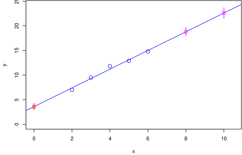
The expectations about the future measurements are instead
| (219) | |||||
| (220) | |||||
| (221) |
with interesting correlations:
- •
, positive and quite high, because their are “on the same side” of the ’experimental’ points and quite close to each other: due to the uncertainty about the slope they could be both smaller or larger than expected.
- •
, negative for the opposite reason, and in absolute value increasing with the distance.
Note how the uncertainty on and are the same, because the corresponding values (8 and 0, respectively) are equally distant, from the barycenter the data along the axis. Instead, is different from because they are not the same thing(!): the uncertainty is a parameter of the model, while is what we would measure at on the base of the information provided by the previous measurements (and our assumptions about the model).
10.2 Uncertainty about Vs uncertainty about
The expected ’s at different values of are
simply the values calculated at different , as it is
easy to check
> out$mu[1] + out$mu[2]*x.f
[1] 18.800001 22.600001 3.599999
More intriguing are the uncertainties.
Indeed they get a contribution from the uncertainty of the
true value and that due to the experimental error
around it.
As far as the true values, in our simplified model they are given by , which we can rewrite in matrix form as
Here are then their expected values and covariance matrix directly in R
> ( C.mu.f <- cbind(rep(1,3), x.f) )
       x.f
[1,] 1   8
[2,] 1  10
[3,] 1   0
>  ( mu.f <- as.vector( C.mu.f %*% out$mu[1:2] ) )
[1] 18.800107 22.600169  3.599857
> ( V.mu.f <- C.mu.f %*% out$V[1:2,1:2] %*% t(C.mu.f) )
           [,1]       [,2]       [,3]
[1,]  0.4499903  0.6499837 -0.3499832
[2,]  0.6499836  0.9499730 -0.5499737
[3,] -0.3499829 -0.5499734  0.4499788
>  ( sigma.mu.f <- sqrt(diag(V.mu.f)) )
[1] 0.6708132 0.9746656 0.6708046
We have then
| (231) | |||||
| (232) | |||||
| (233) |
with exactly equal to the intercept.
And again, the uncertainties on
and are the same,
and then equal to .2525
25
Under
the conditions we are considering here, one can prove that
with the uncertainties depending on the
absolute value of and on the ‘lever arm’
of the experimental date (the larger is their
‘momentum of inertia’, that is ,
the better is the determination of the slope and then
more accurate the extrapolations.
In our case this expression gives
> var.x <- sum(xˆ2)/n - mean(x)ˆ2
> sqrt(syˆ2/n + (x.f-mean(x))ˆ2/var.x*syˆ2/n )
[1] 0.6708204 0.9746794 0.6708204
practically equal to the results got playing with
covariance matrices.
Note that above formula takes into account
the correlation coefficient between and . Without it
we would get
> sqrt(sigmas[1]ˆ2 + x.fˆ2*sigmas[2]ˆ2)
[1] 1.4317521 1.7175207 0.6708046
with and
wrong by about a factor 2
(while is right ‘by chance’,
being equal to the intercept).
(The slight numeric difference at the 5th decimal digit
is due to the effect of the prior, not taken into account in the
the above formula.)
The reason while the uncertainties about are larger than those of , for the same , is also easy to understand. To the uncertainty about the true value we have to add that due to the experimental error. And in a linear model like ours the two contributions add in quadrature, as it easy to check
while and have the standard uncertainty slightly smaller than those of the corresponding and . To obtain these latter standard uncertainties it is enough to add quadratically the standard deviation of the experimental error:
>  sqrt(sigma.mu.f^2 + sy^2)
[1] 0.8366542 1.0954328 0.8366473
The effect of the experimental errors is also to dilute the correlations, which among the true values are
>  V.mu.f / outer(sigma.mu.f, sigma.mu.f)
           [,1]       [,2]       [,3]
[1,]  1.0000000  0.9941347 -0.7777671
[2,]  0.9941347  1.0000000 -0.8411826
[3,] -0.7777666 -0.8411821  1.0000000
10.3 Follows up
Also in this case one do several other instructive test, which we read to the reader. Here is a partial list.
- •
Impose a precise value for the intercept and the slope, to see how the other parameter changes. This can be done, for example for the intercept () with the following conditioning:
> out <- norm.mult.cond(mu, V, c(3, NA, y, NA, NA, NA), full=FALSE)
(Quick test: what would you expect for ?) - •
Do the same test, but using the previous out$V and out$mu.
- •
Use some informative priors for , or both.
- •
Make a new fit on another 5 data points generated from the same model, using as priors for and the result of the previous inference (including the correlation!).
- •
Make a global fit on the 10 data points of the two datasets (starting from uninformative priors) and compare with the result of the two inferences in sequence.
Then is the question of estimating the common standard deviation of the model from the data. As told above, this cannot be done with the tools we are playing in this paper because the problem is not linear. Certainly a rough estimate can be done by the residuals, but if the number of data points is ‘small’ the uncertainty on the estimated sigma do not only affect this parameter, but also the joint pdf of and , which is longer normal bivariate (with consequences on the pdf’s of the previsions). The problem has to be solved using a model without short cuts and making the integrals numerically or by Markov Chain Monte Carlo, issues which are beyond the aim of this paper. (And pay attention to covariance matrices obtained by linearization! [8])
11 Propagation of evidence – some general remarks
Let us take again the diagrams (‘graphs’) which describe two observations from the same true value and one observation resulting from a true value and a systematic effect. They are show again in Fig. 16,
|
|
 |
| (Divergent) | (Convergent) | (Serial) |
labelled with names related to the direction of the ‘causation’ arrows, which diverge from a single node or converge towards a single node. The physical interpretation is that, as we have already seen, of a single cause producing two effects, or two causes responsible of a single effect, respectively. Below each graph we have also added the covariance matrix which characterize it, where , and so on.
For completeness we have added in the figure also graph in which the effect is itself cause of another effect (serial connection). Sticking to the simple linear models we are dealing with, the transformation rules of the graph characterize by a serial connection are the following:
| (234) | |||||
| (235) | |||||
| (236) |
from which the joint covariance matrix reported below the diagram follows, with and .
Analyzing the covariance matrix of the graphs with divergent and serial connections we see that the variables are fully correlated: any evidence on any of the three variables changes the pdf of the other two.
Instead, in the convergent graph and are independent. Indeed, why should the physical quantity we are going to measure should depend on a calibration constant of our detector? And the other way around.2626 26 In reality this is not impossible, but definitely unusual But we have already seen in the examples that if we observe , then and become anticorrelated.
The effect of the propagation of a condition (‘instantiation’) of one variable to the rest of the network is very interesting also for its practical applications, because it allows to decompose a large network in subnetworks.
11.1 Diverging connection
 |
 |
 | ||
 |
 |
 |
We have already seen in the numerical examples of subsection 5.1 that if we condition on a value of , then and become independent, and the physical reason was very easy to be understood. This is a general property of divergent graphs, usually stated referring to parents and children: in a divergent graph, if a parent is instantiated, the children become independent, i.e. evidence does not flow any longer from one child to the other (‘an instantiated parent blocks evidence flow among children’ – we assume that there is no other connection among them!). The possible flows of evidence are reported in figure 17.
Let us make the exercise to calculate the covariance matrix of and given . To use Eq. 52 we need to rewrite the three variables in a compact form, thus defining and . In this case it is convenient to rewrite (52) swapping the indices, thus obtaining:
| (237) |
with
| (244) | |||||
| (245) | |||||
It follows
and hence
As expected, the exercise shows that and have become conditionally independent.
 |
 |
 | ||
 |
 |
11.2 Converging connection
Instead, in the case of a converging connection, the parents are initially independent. That is the evidence on either parent, or on both, can influence the child(s), but cannot be transmitted from one parent to the other, as depicted in the graphs of figure 18. Let us make the exercise of instantiating the child, .
In this case the convenient partition is and , and the conditional covariance matrix is obtained applying directly Eq. (52):
| (257) |
with
| (264) | |||||
| (265) | |||||
It follows
and hence
As expected, the exercise shows that and become anticorrelated, although the correlation coefficient has not a simple intuitive explanation.
11.3 Serial connection
Let us repeat the exercise for the serial connection, depicted in figure 19.
 |
 |
 |
 |
 |
 |
The convenient partition is now and . And these are the details
| (288) | |||||
| (289) | |||||
It follows
and hence
As expected, the exercise shows that and become now independent and the uncertainty about is simply . And also in we recognize a familiar pattern (see also footnote 15):
| (303) |
References
- [1]
C.F. Gauss, “Theoria motus corporum coelestium in sectionibus
conicis solem ambientum”, Hamburg 1809, n.i 172–179; reprinted
in Werke, Vol. 7 (Gota, Göttingen, 1871), pp 225–234.
(See e.g. in http://www.roma1.infn.it/~dagos/history/GaussMotus/index.html) - [2] R Core Team (2013). R: A language and environment for statistical computing. R Foundation for Statistical Computing, Vienna, Austria. URL http://www.R-project.org.
- [3] M. Eaton, Multivariate Statistics : A Vector Space Approach, John Wiley and Sons 1983 (available at http://projecteuclid.org/).
- [4] See e.g. http://www.cs.unc.edu/~welch/kalman/.
- [5] G. D’Agostini, Bayesian reasoning in data analysis – a critical introduction, World Scientific 2003.
- [6] G. Cowan, Statistical data analysis, Clarendon Press, 1998.
- [7] G. D’Agostini, Fits, and especially linear fits, with errors on both axes, extra variance of the data points and other complications, arXiv:physics/0511182.
- [8] G. D’Agostini, On the use of the covariance matrix to fit correlated data, Nucl. Instrum. Methods. A346 (1994) 306.