A mass conservative generalized multiscale finite element method applied to two-phase flow in heterogeneous porous media
Abstract
In this paper, we propose a method for the construction of locally conservative flux fields through a variation of the Generalized Multiscale Finite Element Method (GMsFEM). The flux values are obtained through the use of a Ritz formulation in which we augment the resulting linear system of the continuous Galerkin (CG) formulation in the higher-order GMsFEM approximation space. In particular, we impose the finite volume-based restrictions through incorporating a scalar Lagrange multiplier for each mass conservation constraint. This approach can be equivalently viewed as a constraint minimization problem where we minimize the energy functional of the equation restricted to the subspace of functions that satisfy the desired conservation properties. To test the performance of the method we consider equations with heterogeneous permeability coefficients that have high-variation and discontinuities, and couple the resulting fluxes to a two-phase flow model. The increase in accuracy associated with the computation of the GMsFEM pressure solutions is inherited by the flux fields and saturation solutions, and is closely correlated to the size of the reduced-order systems. In particular, the addition of more basis functions to the enriched multiscale space produces solutions that more accurately capture the behavior of the fine scale model. A variety of numerical examples are offered to validate the performance of the method.
Keywords:
Generalized multiscale finite element method, high-contrast permeability, two-phase flow, Lagrange multipliers1 Introduction and problem statement
In this paper, we primarily consider the equation given by
| (1) | |||
where is a heterogeneous field with high contrast. In particular, we assume that there is a positive constant such that , while can have very large values (i.e., is large). Additionally, is a known mobility coefficient, denotes any external forcing, and is an unknown pressure field satisfying Dirichlet and Neumann boundary conditions given by and , respectively. Here a convex polygonal and two dimensional domain with boundary .
Let us consider a function in whose trace on coincides with the given value ; we denote this function also by . The variational formulation of problem (1) is to find with and such that
| (2) |
where, for , the bilinear form is defined by
| (3) |
the functional is defined by
| (4) |
and the linear functional related to the boundary condition is given by
| (5) |
A main goal of our work is to obtain conservative discretizations of the equations above. More specifically, construction of approximation that satisfy some given conservation of mass restriction on subdomains of interest. We note that a popular conservative discretization is the Finite Volume (FV) method. The classical FV discretization provides and approximation of the solution in the space of piecewise linear functions with respect to a triangulation while satisfying conservation of mass on elements of a dual triangualtion. When the approximation of the piecewise linear space is not enough for the problem at hand, advance approximation spaces need to be used. However, in some cases this requires a sacrifice of the conservation properties of the FV method. In this work we present an extension of the FV method for general approximation spaces that enrich classical approximation spaces (such as the space of piecewise linear functions). In particular, this conservative discretization can be used in conjunction with recently introduced GMsFEM spaces.
We note that FV methods that use higher degree piecewise polynomials have been introduced in the literature. The fact that the dimension of the approximation spaces is larger than the number of restrictions led the researchers of [1, 2] to introduce additional control volumes to match the number of restrictions to the number of unknowns. An alternative approach is to consider a Petrov-Galerkin formulation with additional test functions rather that only piecewise constant functions on the dual grid. They where able to obtain stability of the method as well as error estimates. It is important to observe that the additional control volumes require additional computational work to be constructed and in some cases are not easy to construct (see also [3, 4]). Additionally, it is well know that piecewise smooth approximations spaces do not perform well for multiscale high-contrast problems [5, 6, 7, 8, 9, 10, 11, 12]. Another technique that one can use in order obtain a conservative method with richer approximations spaces is the following (see for instance [20] where the authors use a similar approach). In the discrete linear system obtained by a finite element discretization, it is possible to substitute appropriate number of equations by finite volume equations involving only the standard dual grid. This approach has the advantage that no additional control volume needs to be constructed. It may have the flexibility of both FV and FE procedures given as mass conservative fluxes and residual minimization properties. Some previous numerical experiments suggest a drawback of this approach - the resulting discrete problems may be ill-conditioned for large dimension coarse spaces, specially for higher order approximation spaces and multiscale problems.
In this paper we propose the alternative of using a Ritz formulation and construct a solution procedure that combines a continuous Galerkin-type formulation that concurrently satisfies mass conservation restrictions. To this end, we augment the resulting linear system of the Galerkin formulation in the higher order approximation space to impose the finite volume restrictions. In particular, we do that by using a scalar Lagrange multiplier for each restriction. This approach can be equivalently viewed as a constraint minimization problem where we minimize the energy functional of the equation restricted to the subspace of functions that satisfy the conservation of mass restrictions. Then, in the Ritz sense, the obtained solution is the best among all functions that satisfy the mass conservation restriction.
As a main application of the techniques presented here, we consider the case where the coefficient has high-variation and discontinuities (not necessarily aligned with the coarse grid). For this problem it is known that higher order approximation is needed. Indeed, in some cases robust approximation properties, independent of the contrast, are required. See for instance [8, 9, 10] where it is demonstrated that classical multiscale methods ([13]) do not render robust approximation properties in terms of the contrast. It is shown that one basis functions per coarse node (with the usual support) is not enough to construct adequate coarse spaces [9, 14]. A similar issue can be expected for the multiscale finite volume method developed in [15, 16, 17] and related works, when applied to high-contras multiscale problems since the approximation spaces have similar approximation properties. In the case of Galerkin formulations, robust approximation properties are obtained by using the Generalized Multiscale Finite Element Method (GMsFEM) framework. The main goal of GMsFEMs is to construct coarse spaces for Multiscale Finite Element Methods (MsFEMs) that result in accurate coarse-scale solutions. This methodology was first developed in [5, 6, 7] based on some previous works [8, 9, 10, 11, 12]. A main ingredient in the construction is the use of an approximation of local eigenvectors (of carefully selected local eigenvalues problem) to construct the coarse spaces. Instead of using one coarse function per coarse node as in classical MsFEM, in the GMsFEM it was proposed to use several multiscale basis functions per coarse node. These basis functions represent important features of the solution within a coarse-grid block and they are computed using eigenvectors of an eigenvalue problem. For applications to high-contras problems, methodologies to keep small the dimension of the resulting coarse space where successfully proposed ([9]). That paper made use of coarse spaces that somehow incorporated important modes of a (local) energy related to the problem motivated the general version of the GMsFEM. The much more general GMsFEM was then developed in [5] where several more practical options to compute important modes to be include in the coarse space were used; see also [18] for an earlier construction. It is important to mention that the methodology in [5] was designed for parametric and nonlinear problems and can be applied in variety of applications, although a more extensive review of such developments is not contained herein.
An important consideration of the proposed method is that the GMsFEM methodology does not guarantee conservation of mass properties such as those of Finite Volume formulations. In this paper we design a mass conservative GMsFEM method. In particular, we impose the mass conservation constraints over control volumes by using Lagrange multipliers. In doing so, we numerically validate that the convergence properties of the GMsFEM are maintained while the approximate solution simultaneously satisfies the required conservation properties. We mention that in [19] some successful applications of GMsFEM to two-phase problems were presented. In that work, the authors developed a technique in which GMsFEM solutions could be post-processed to yield mass conservative fluxes for use in two-phase modeling. While the motivation of the previous work in [19] is similar, the current technique yields a system that requires no post-processing, and a solution that automatically yields conservation. In particular, in the present work no additional equations must be solved (in notable constrast to [19]) in order to ensure coarse-grid conservation, as a single global solve automatically yields the desired properties. As a result, no additional computational resources must be allocated, and issues such as ill-conditioning of the localized systems may be circumvented. Additionally, the proposed method ensures that the solution obtained through the method proposed in this work is the best among all functions (in the Ritz sense) satisfying the mass conservation restrictions.
Finally we mention the works on MsFV. When dealing with multiscale problems, the lack of accuracy in the use of classical spaces had led researchers to introduce enriched spaces (as well as iterative procedures). In [20] the authors construct an enrichment of the initial coarse space spanned by nodal basis functions. We also note that a hybrid finite-volume/Galerkin formulation for the coarse-scale problem is devised. The authors show that the resulting method has all features of the MsFV method, but is more robust and shows improved convergence properties if used in an iterative procedure. In comparison, in this work we use a GMsFEM framework were the additional degrees of freedom are related to local eigenvalue problems. This construction is related to the approximation properties the resulting space will have and is motivated by the numerical analysis of the interpolation operator into the coarse space. Furthermore, instead of a hybrid finite-volume/Galerkin formulation, we employ a Ritz formulation in the space of functions satisfying the conservation of mass.
The rest of the paper is organized as follows. In Section 2, we recall how to impose restrictions using Lagrange multipliers in general and, in particular, for the mass conservation restrictions. In Section 3 we formulate a conservative coarse problem that follows the framework of Section 2. Section 4 is dedicated to present some relevant discussions for the case of smooth coefficients and solutions. In Section 5 we present the two-phase flow model problem and the overall solution algorithm. In Section 6 we summarize some basic construction topics associated with the GMsFEM methodology. In Section 7 we present some representative numerical results to illustrate the successful performance of our method for the case of single- and two-phase flow problems in high-contrast heterogeneous porous media. Some concluding remarks are finally offered in Section 8.
2 Linear restrictions using Lagrange Multipliers
Problem (2) is equivalent to the minimization problem: Find with and such that
| (6) |
where the minimum is taken over such that and
| (7) |
Let be the solution of (2) and , , be continuous linear functionals on . Define , . The problem above is equivalent to: Find such that
| (8) |
where
Problem (8) above can be view as Lagrange multipliers min-max optimization problem. See [21] and references therein.
Then, in case an approximation of , say , it is required to satisfy the constraints , , we can discretize directly the formulation (8). In particular, we can apply this approach to a set of mass conservation restrictions used in finite volume discretizations.
2.1 Mass conservation in fine control volumes
In order to ensure fine-scale conservation, we start by selecting control volumes We assume that each is a subdomain of with polygonal boundary and . If we have that (2) is equivalent to: Find with and such that
| (9) |
where the subset of functions that satisfy the mass conservation restrictions is defined by
The Lagrange multiplier formulation of problem (8) can be written as: Find with and that solves,
| (10) |
Here, the average flux bilinear form is defined by
| (11) |
The functional is defined by
The first order conditions of the min-max problem above give the following saddle point problem: Find with and that solves,
| (12) |
See for instance [21].
3 Conservative discrete coarse problem
Let be a coarse-mesh parameter and be a coarse-scale triangulation. We assume that does not necessary resolve all the variation of the coefficient. In what follows we introduce the finite element space associated with the coarse resolution . In applications concerning heterogeneous multiscale media, the standard finite element spaces on do not offer good approximation properties and therefore some special enrichment of this space is needed in order to achieve some acceptable approximation properties.
We denote by the vertices of the coarse mesh and define the neighborhood of the node by
| (13) |
See Fig. 1 for an illustration of the coarse-scale discretization depicting coarse neighborhoods and control volumes.
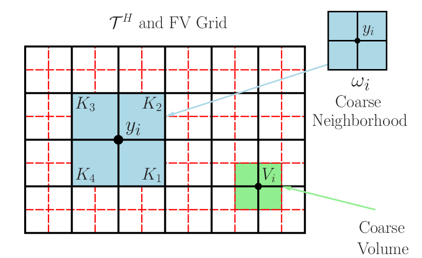
Using the coarse mesh we introduce a set of coarse basis functions . The basis functions are supported in ; however, for one specific neighborhood , there may be multiple basis functions. We define the associated coarse space by
| (14) |
Let be a discrete interpolation of the boundary data . The classical multiscale solution of (2) is given by with such that
| (15) |
where the minimum is taken over the set of with . The equivalent matrix form of the Ritz-Galerkin formulation (15) is given by
| (16) |
where the coarse matrix and the coarse load vector are such that for all we have
| (17) |
The multiscale solution of problem (16) does not necessarily have any conservation of mass property. Therefore, the classical multiscale solution might not be appropriate form some applications where it is imperative that approximations have some conservation properties in the form of average flux through some control volumes. To obtain multiscale solutions with the required conservation properties one can proceed as described in Section 2. To that end, we let be defined as before and consider the set of all discrete functions that satisfy the required approximation properties,
where denotes a coarse dual-grid volume.
We then consider the following discrete formulation that takes into account the required restrictions. The approximation of the solution of (1) is to find such that
| (18) |
This is a minimization problem with linear constraints similar to (8) - Indeed, it is the associated Ritz-Galerkin formulation; see Section 2. This problem can be equivalently written in the form analogous to (10) or (12). The matrix formulation stating the first order conditions of this minimization problem is written as
| (19) |
where the matrix and the vector are defined in (17) and the finite volume matrix is defined by
4 The case of smooth solutions
In this section, in order to motivate the use of the the formulation (18) for multiscale problems, we make some comments on the method described so far for the case of smooth coefficients and higher-order degree polynomials for finite volume methods.
As mentioned in the introduction, when higher order degree polynomials are used within a finite volume framework one can proceed in different ways. Let us assume, only for this section and with motivation purposes, that is the space of piecewise polynomials with . Let us then introduce the dual grid . The dimension of the approximation space is higher that the number of controls volumes or dual elements. The number of control volumes matches the dimension of the subspace of piecewise linear functions contained in . When and if we use only piecewise constant functions on the dual grid as a test function we do not obtain a square system. In order to obtain a square linear system one have to introduce additional test functions. One can proceed as follows.
- 1.
Construct additional control volumes and test the approximation spaces against piecewise constant functions over the total of control volumes (that include the dual grid element plus the additional control volumes). We mention that constructing additional control volumes is not an easy task and might be computationally expensive. We refer the interested reader to [1, 22, 2] for additional details.
- 2.
Use as additional the basis functions the basis functions that correspond to nodes other than vertices to obtain a FV/Galerkin formulation. This option has the advantage that no geometrical constructions have to be carried out. On the other hand, this formulation seems difficult to analyze. Also, some preliminary numerical tests suggest that the resulting linear system becomes unstable for higher order approximation spaces (especially for the case of high-contrast multiscale coefficients).
- 3.
Use the Ritz formulation with restrictions (18).
Note that if , in the linear system associated to (19), the restriction matrix corresponds to the usual finite volume matrix. This matrix is known to be invertible. In this case, the affine space is a singleton. Moreover, the only function satisfying the restriction is given by . The Ritz formulation (18) reduces to the classical finite volume method.
If we switch to , the dimension of the space can only increase. Therefore and due to ellipticity of the energy functional, the Ritz formulation with restrictions
(18) makes sense and it will give the best approximation of the
solution in the space of functions that satisfy the restrictions. Then, in the Ritz sense, the solution of
(18) is not worse that any of the solutions obtained by
the methods 1. or 2. mentioned above. Furthermore, the solution of the associated linear system
(19), which is a saddle point linear system, can be readily implemented using
efficient solvers for the matrix (or efficient solvers for the classical finite volume matrix );
See for instance [21].
Additionally, we mention that the analysis of the method can be carried out using usual tools for the analysis of
restricted minimization of energy functionals and mixed finite element methods. The numerical analysis of our methodology
is under current investigation and it will presented elsewhere.
The comments and observations of this section are the main motivation for the methodology developed here to target fluid flow in porous media where, as it is well known, advanced and sophisticated approximation spaces have to be used. Furthermore, in some applications such as multiphase flow, conservation of mass is a main requirement.
5 Two-phase model problem
We emphasize that solving the pressure equation in (1) is done within the context of a two-phase flow model. In particular, we are interested in treating a problem confined to a domain in which the subsurface is assumed to exhibit high-contrast features. The heterogeneous reservoir is equipped with a well in which water is injected to displace the trapped oil towards the production wells. The water and oil phases (which we denote by and , respectively) are assumed to be immiscible, and we consider a gravity-free enviroment in which the pore space of the reservoir is fully saturated. Additionally, we assume that any capillary effects are negligible. Under such assumptions, combining Darcy’s law with a statement of conservation of mass yields governing equations of the form
| (20) |
where the total Darcy velocity is given by
| (21) |
The pressure equations given by (20) is coupled to a transport equation
| (22) |
where denotes the water saturation, and denote any external forcing. The total mobility coefficient and flux function are respectively given by
where is the relative permeability of the fluid phase.
5.1 Solution algorithm
In order to solve the coupled two-phase model given in Eqs. (20), (21), and (22) we employ an operator splitting technique where the saturation from the previous time step is used to update the mobility coefficient required of the pressure solve and subsequent velocity calculation (see, e.g., [23]). Once this velocity is available, it is used in conjunction with an explicit saturation time-marching scheme for a specified number of time steps. The updated saturation is used again in order to update the pressure, and the process is continued until a final simulation time is reached. See Fig. 2 for a schematic of the the operator splitting.

To discretize the saturation equation, we integrate Eq. (22) with respect to time, and then over some volume . Applying the left end-point quadrature rule to a second term in time, and integrating by parts yields the following expression
where the errors terms have been neglected and
In addition to the explicit time stepping in the above expression, we apply a non-oscillatory upwinding scheme on the flux term (see, e.g., [24] for a review of upwinding schemes on rectangular meshes). As mentioned in Section 2, it is crucial that that the numerical flux approximation satisfies a local conservation property. In particular, we wish to seek discrete solutions that satisfy
| (23) |
We emphasize that a main consideration of this paper is to ensure the conservation property in (23) through the use of Lagrange multiplier restrictions (refer to Section 2) within a suitable coarse-scale solution space (refer to Section 3). In turn, in the next section we describe the systematic construction of the Generalized Multiscale Finite Element Method (GMsFEM) coarse solution space.
6 Generalized multiscale finite element method
In this section we focus on high-contrast multiscale problems and summarize a GMsFEM construction of used in Section 3. For a more detailed description of the development of the GMsFEM methodology, see [5, 6, 7] and references therein.
6.1 Spectral enrichment
We start by chosing and initial set of basis functions that form a partition of unity. The space generated by this basis functions is enriched using a local spectral problem. We use the multiscale basis functions partition of unity with linear boundary conditions ([13]). We have one function per coarse-node and it is defined by
| (24) | |||||
where is a standard linear partition of unity function.
For each coarse node neighborhood , consider the eigenvalue problem
| (25) |
with homogeneous Neumann boundary condition on . Here and are eigenvalues and eigenvectors in and is defined by
| (26) |
We use an ascending ordering on the eigenvectors,
Using the partition of unity functions from Eq. (24) and eigenfunctions from Eq. (25), we then construct a set of enriched multiscale basis functions given by for selected eigenvectors . Using to denote the number of basis functions from the coarse region , we then define the coarse GMsFEM space by
For more details, motivation of the construction, and approximation properties of the space as well as the choice of the initial partition of unity basis functions we refer the interested reader to [5, 6, 7].
Summarizing, in order to solve problem (1) for the pressure we use the GMsFEM coarse space constructed in this section. Additionally, in order to obtain conservative solutions with respect to a dual coarse grid, we use the discretization presented in Section 3. In particular, we solve the saddle point problem (19) using the appropriate approximation spaces and conservation constraints. We also recall Section 5 for a description the overall solution algorithm used to solve the two-phase flow problem.
6.2 A flux downscaling procedure
At this point we carefully distinguish the scales at which we wish to calculate respective flux values. Recalling the discussions from Section 2.1 and Section 3, we note that sets of control volumes or are selected in order to incorporate the associated mass conservation restrictions of the fine and coarse problems, repsectively. In the case of the fine-scale problem, we simply assume that the set of control volumes coincides with the nodal values of the mesh. In particular, the conservation constraints are taken directly on the fine scale. The case when we use GMsFEM is similar in the sense that we initially impose the constraints on the (larger) volumes associated with the coarse mesh discretization (see Fig. 1). As such, a global GMsFEM-FV solve directly yields flux parameters that satisfy a coarse analogue of conservation. While this level of conservation may hold for some target applications (see, e.g., [25]), in this paper we wish to construct fluxes that are conservative directly on the fine scale for a direct means of comparison with the fine-scale FV technique.
In constructing fine-scale mass conservative fluxes, we recall that the coarse solve from Section 3 yields the coarse conservation property
which can analogously be thought of as the compatibility condition in . As such, we may formulate a fully Neumann boundary value problem
| (27) | |||
where the known is evaluated pointwise on the boundaries . In particular, after obtaining the coarse solution and the coarse-scale conservative flux , we solve the set of localized problems in Eq. (27) for every in using any method that produces the desired fine-scale conservation. For consistency within this paper, we use the fine-scale FV technique to ensure fine conservation. A hallmark advantage of the downscaled post- processing procedure from (27) is that the localized problems are independent from one another. In particular, the problems are naturally parallelizable (as should also be carefully noted for Eqs. (24) and (25)), and may be independently distributed to CPU and/or GPU multi-core clusters for a significant gain in computational efficiency [26].
7 Numerical results
In this section we offer a variety of numerical examples to test the performance of the method introduced in Section 2. In particular, we solve the model problem in Eq. (1) using the constrained discretization techniques from Sections 3 and 6. A main goal is to address the accuracy associated with the reduced- order conservative GMsFEM approach as compared to the fine-scale FV approach.
7.1 Single-phase pressure
For the first set of examples, we employ both the fine-scale FV and GMsFEM-FV approaches to solve Eq. (1). Throughout the section we consider solutions that are obtained through solving the equation on the unit square domain . We impose boundary conditions of and on the left and right boundaries of the domain, along with no-flow (i.e., zero Neumann) conditions on the top and bottom. The fine coefficient (and reference solution) are posed on a fine mesh that yields a global system of size . See Fig. 3 for an illustration of high-constrast structure that is considered in this section. More specifically, the system from Eq. (19) is of size , where denotes the dimension of the space in which the fine-grid pressure solution is represented, and denotes the number of dual-grid volumes where the finite volume constraints are imposed. In constructing the coarse-grid solutions in this section, we consider a coarse mesh with varying levels of constrained spectral enrichment. In particular, we obtain systems of size where denotes the number of degrees of freedom associated with the coarse enrichment, and denotes the number of coarse dual-grid volumes where the associated finite volume constraints are imposed. For this set of examples we emphasize that the number of coarse dual-grid volume constraints is fixed at , which corresponds to the number of coarse nodal values (and surrounding volumes) of the domain (cf. Fig. 1).

As an initial motivation, we offer a comparison of single-phase pressure solutions in Fig. 4. The coarse solutions in Figs. 4(b) and 4(c) were obtained through solving the global equation using two levels of coarse mesh enrichment. We can see from Fig. 4(b) that a system of size offers a somewhat crude approximation to the reference solution, yet that a system of size (cf. Fig. 4(c)) yields a solution that is nearly indistinguishable from the reference solution. In either case, we emphasize that the coarse systems are much smaller than the system of size that is used to obtain the fine-grid reference solution.


For more rigorous comparisons we also consider the relative error quantities given by
| (28) |
where denotes the reference fine-grid solution, is a specified coarse-grid (GMsFEM-FV) solution. For the norm quantities in (28), we consider both the energy and weighted norms respectively given by
We note that the energy error is of particular importance for the analysis associated with GMsFEM (see, e.g., [5]), and involves the gradient of the solution (which offers a flux- like comparison). However, using either norm we are primarily interested in illustrating the effects of larger coarse spaces (i.e., more basis functions) in the GMsFEM-FV construction. In Table 1 we offer a number of errors corresponding to a variety of coarse space dimensions. The left most column tabulates the total size of the full coarse system associated with a specified level of enrichment and conservation constraints. The next two columns itemize the dimension of the coarse space (and corresponding number of basis functions per coarse node), and the number of FV constraints. Most importantly, the results indicate that an increase in the coarse-space dimension yields a predictable error decline associated with the solution and its gradient. As such, these results strongly suggest that incorporating numerous pressure solves into the context of the operator splitting technique (recall Section 5.1) will yield increasingly accurate two-phase saturation solutions. This is what we consider in the next subsection.
| Full System | Coarse Dimension | Constraints | Relative Errors (%) | |
|---|---|---|---|---|
| [ basis] | ||||
| 242 | 121 [1] | 121 | 8.4 | 100 |
| 323 | 202 [2] | 121 | 7.4 | 39.8 |
| 485 | 364 [4] | 121 | 1.2 | 15.0 |
| 647 | 526 [6] | 121 | 0.9 | 11.1 |
| 809 | 688 [8] | 121 | 0.3 | 9.0 |
| 971 | 850 [10] | 121 | 0.3 | 8.1 |
7.2 Two-phase saturation
In this section we apply the constrained GMsFEM method to the full two-phase model as described in Section 5. More specifically, we apply the conservative GMsFEM discretization of Eq. (1) for each pressure update. Then, a fine scale conservative flux field is obtained via the downscaling procedure in Section 6.2 in order to march the saturation solution in time using the explicit scheme from Section 5.1. In doing so, we assess the effectiveness of the proposed approach in a context where it is repeatedly used to accurately capture a number of pressure equation updates.
To solve the two-phase model given in Eqs. (20) and (22) we use quadratic relative permeability curves given by and . We additionally use values of and for the water and oil phase viscosities. The same pressure boundary conditions from Section 7.1 are used, and for the initial saturation condition, we set at the left edge and assume elsewhere. Finally, we recall that the high-contrast permeability coefficient illustrated in Fig. 3 is used for . For a motivating application of the method, we offer a representative set of two-phase flow solutions in Fig. 6. The plot shows saturation solutions advancing in time for a variety of coarse space dimensions, compared with fine-scale reference solutions. In particular, the first row shows three saturation snapshots for the case when , and the second, third and fourth rows respectively shows saturation snapshots for the cases when . We note a significant improvement for the case when as compared to the lower dimension . More specifically, the addition of more basis functions to the coarse pressure space yields flux and saturation values that accurately capture the fine-scale behavior of the system. And, with respect to the reduced dimension , we can see that the solutions are nearly indistinguishable from the reference solutions.

For a final set of comparisons, we tabulate the standard relative error of the saturation profiles from Fig. 6, as well as for a variety of other scenarios. The full set of results can be seen in Fig. 7. For these examples, we use a variety of coarse-space dimensions and and run the simulations to a final time of . A time stepping value of is used, and we update the saturation for time steps in between each pressure solve. As was evident from the previous illustration, we can see from Fig. 7 that the error may be significantly decreased by adding more basis functions in the GMsFEM construction. As a particular example, a maximum error value of roughly () may be decreased to a maximum error value of roughly in the case when . These results serve to further illustrate the flexibility and accuracy associated with the conservative GMsFEM construction. More specifically, more basis functions may be used to obtain a higher level of accuracy, whereas less basis functions may be used when efficiency is a main consideration.

8 Concluding remarks
In this paper, we propose a method for the construction of locally conservative flux fields through a constrained variation of the Generalized Multiscale Finite Element Method (GMsFEM). The flux values are obtained through the use of a Ritz formulation in which we augment the resulting linear system of the continuous Galerkin (CG) formulation in the higher-order GMsFEM approximation space. We impose the finite volume-based restrictions through incorporating a scalar Lagrange multiplier for each mass conservation constraint on a specified scale, and as such, the proposed method may be viewed as a minimization problem in which an energy functional of the governing equations is minimized within a subspace of functions that satisfy the desired conservation properties. Due to the inherent construction of the coarse-grid solution space, and the way in which the mass conservation constraints are imposed, the combined methodology is shown to offer a robust and flexible framework for obtaining conservative flux fields to be used in two-phase flow modeling. To illustrate the performance of the method we consider model flow equations with heterogeneous permeability coefficients that have high-variation and discontinuities which significantly affect the flow patterns of the two-phase model. The increase in accuracy associated with the computation of the GMsFEM pressure solutions is inherited by the flux fields and saturation solutions, and is closely correlated to the size of the reduced-order systems. In particular, the addition of more basis functions to the enriched multiscale space produces solutions that more accurately capture the behavior of the fine scale model. A variety of single- and two-phase numerical examples are offered to validate the performance of the method.
Acknowledgments
J. Galvis would like to thank R. Lazarov and P. Chatzipantelidis for interesting discussions on higher order finite volume methods and for pointing out some of the references. M. Presho is supported by the U.S. Department of Energy Office of Science, Office of Advanced Scientific Computing Research, Applied Mathematics program under Award Number DE-SC0009286 as part of the DiaMonD Multifaceted Mathematics Integrated Capability Center.
References
References
- [1]
L. Chen, A new class of high order
finite volume methods for second order elliptic equations, SIAM J. Numer.
Anal. 47 (6) (2010) 4021–4043.
doi:10.1137/080720164.
URL http://dx.doi.org/10.1137/080720164 - [2]
Z. Chen, J. Wu, Y. Xu,
Higher-order finite volume
methods for elliptic boundary value problems, Adv. Comput. Math. 37 (2)
(2012) 191–253.
doi:10.1007/s10444-011-9201-8.
URL http://dx.doi.org/10.1007/s10444-011-9201-8 - [3]
P. Chatzipantelidis, Finite
volume methods for elliptic PDE’s: a new approach, M2AN Math. Model.
Numer. Anal. 36 (2) (2002) 307–324.
doi:10.1051/m2an:2002014.
URL http://dx.doi.org/10.1051/m2an:2002014 - [4]
M. Plexousakis, G. E. Zouraris,
On the construction and
analysis of high order locally conservative finite volume-type methods for
one-dimensional elliptic problems, SIAM J. Numer. Anal. 42 (3) (2004)
1226–1260 (electronic).
doi:10.1137/S0036142902406302.
URL http://dx.doi.org/10.1137/S0036142902406302 - [5] Y. Efendiev, J. Galvis, T. Hou, Generalized multiscale finite element methods, Journal of Computational Physics 251 (2013) 116–135.
- [6] Y. Efendiev, J. Galvis, X. H. Wu, Multiscale finite element methods for high-contrast problems using local spectral basis functions, Journal of Computational Physics 230 (4) (2011) 937–955.
- [7] Y. Efendiev, J. Galvis, G. Li, M. Presho, Generalized multiscale finite element methods. oversampling strategies, International Journal for Multiscale Computational Engineering 12 (6) (2014) 465–485.
- [8] J. Galvis, Y. Efendiev, Domain decomposition preconditioners for multiscale flows in high contrast media, SIAM J. Multiscale Modeling and Simulation 8 (2010) 1461–1483.
- [9] J. Galvis, Y. Efendiev, Domain decomposition preconditioners for multiscale flows in high contrast media. reduced dimension coarse spaces, SIAM J. Multiscale Modeling and Simulation 8 (2010) 1621–1644.
- [10] Y. Efendiev, J. Galvis, R. Lazarov, J. Willems, Robust domain decomposition preconditioners for abstract symmetric positive definite bilinear forms, ESIAM : M2AN 46 (2012) 1175–1199.
- [11] Y. Efendiev, J. Galvis, E. Gildin, Local-global multiscale model reduction for flows in highly heterogeneous media, Submitted.
- [12] Y. Efendiev, J. Galvis, Coarse-grid multiscale model reduction techniques for flows in heterogeneous media and applications, Chapter of Numerical Analysis of Multiscale Problems, Lecture Notes in Computational Science and Engineering, Vol. 83. 97–125.
- [13] Y. Efendiev, T. Hou, Multiscale Finite Element Methods: Theory and Applications, Vol. 4 of Surveys and Tutorials in the Applied Mathematical Sciences, Springer, New York, 2009.
- [14]
H. Owhadi, L. Zhang, Localized bases
for finite-dimensional homogenization approximations with nonseparated scales
and high contrast, Multiscale Model. Simul. 9 (4) (2011) 1373–1398.
doi:10.1137/100813968.
URL http://dx.doi.org/10.1137/100813968 - [15]
I. Lunati, S. H. Lee, An operator
formulation of the multiscale finite-volume method with correction function,
Multiscale Model. Simul. 8 (1) (2009) 96–109.
doi:10.1137/080742117.
URL http://dx.doi.org/10.1137/080742117 - [16]
R. Künze, I. Lunati, S. H. Lee,
A multilevel multiscale
finite-volume method, J. Comput. Phys. 255 (2013) 502–520.
doi:10.1016/j.jcp.2013.08.042.
URL http://dx.doi.org/10.1016/j.jcp.2013.08.042 - [17]
P. Jenny, S. H. Lee, H. A. Tchelep,
Adaptive multiscale finite-volume
method for multiphase flow and transport in porous media, Multiscale Model.
Simul. 3 (1) (2004/05) 50–64 (electronic).
doi:10.1137/030600795.
URL http://dx.doi.org/10.1137/030600795 - [18] Y. Efendiev, J. Galvis, F. Thomines, A systematic coarse-scale model reduction technique for parameter-dependent flows in highly heterogeneous media and its applications, Multiscale Model. Simul. 10 (2012) 1317–1343.
- [19]
L. Bush, V. Ginting, M. Presho,
Application of a
conservative, generalized multiscale finite element method to flow models,
J. Comput. Appl. Math. 260 (2014) 395–409.
doi:10.1016/j.cam.2013.10.006.
URL http://dx.doi.org/10.1016/j.cam.2013.10.006 - [20] D. Cortinovis, P. Jenny, Iterative galerkin-enriched multiscale finite-volume method, Journal of Computational Physics 277 (15) (2014) 248–267.
- [21]
M. Benzi, G. H. Golub, J. Liesen,
Numerical solution of
saddle point problems, Acta Numer. 14 (2005) 1–137.
doi:10.1017/S0962492904000212.
URL http://dx.doi.org/10.1017/S0962492904000212 - [22]
Z. Chen, Y. Xu, Y. Zhang,
A construction of
higher-order finite volume methods, Math. Comp. 84 (292) (2015) 599–628.
doi:10.1090/S0025-5718-2014-02881-0.
URL http://dx.doi.org/10.1090/S0025-5718-2014-02881-0 - [23] K. Aziz, A. Settari, Petroleum Reservoir Simulation, Applied Science Publishers, 1979.
- [24] J. Thomas, Numerical Partial Differential Equations; Conservation Laws and Elliptic Equations, Springer-Verlag, New York, 1999.
- [25] V. Ginting, F. Pereira, M. Presho, S. Wo, Application of the two-stage Markov chain Monte Carlo method for characterization of fractured reservoirs using a surrogate flow model, Comput. Geosci. 15 (2011) 691–707. doi:DOI10.1007/s10596-011-9236-4.
- [26] T. Hou, X. Wu, A multiscale finite element method for elliptic problems in composite materials and porous media, J. Comput. Phys. 134 (1997) 169–189.