Preconditioning techniques in frame theory and probabilistic frames

We shall investigate frames via the analysis operator, $L$, defined by

The synthesis operator is the adjoint $L^{*}$ of $L$ and is defined by

It is easily seen that the canonical matrix associated to $L^{*}$ is the $N\times M$ matrix whose $k^{th}$ column is the frame vector $\varphi_{k}$. As such we shall abuse notation and denote this matrix by $\Phi$ again. Consequently, the canonical matrix associated with $L$ is simply $\Phi^{T}$, the transpose of $\Phi$.

The frame operator $S=L^{*}L$ is given by

and its matrix will be denoted (again) by $S$ with

The Gramian (operator) of the frame is defined by

In fact, the Gramian in an $M\times M$ matrix whose $(i,j)^{th}$ entry is $\langle\varphi_{j},\varphi_{i}\rangle.$

$\Phi=\{\varphi_{k}\}_{k=1}^{M}\subset\mathbb{R}^{M}$ is a frame if and only if $S$ is a positive definite matrix on $\mathbb{R}^{M}$. In this case,

is also a frame, called the canonical dual frame, and, for each $x\in\mathbb{R}^{N}$, we have

A frame $\Phi$ is a tight frame if we can choose $A=B$. In this case the frame operator is simply a multiple of the identity operator. To any frame $\Phi=\{\varphi_{k}\}_{k=1}^{M}\subset\mathbb{R}^{M}$ is associated a canonical tight frame given by

such that for every $x\in\mathbb{R}^{N}$,

If $\Phi$ is a tight frame of unit-norm vectors, we say that $\Phi$ is a finite unit-norm tight frame (FUNTF). In this case, the reconstruction formula (1.1) reduces to

FUNTFs are one of the most fundamental objects in frame theory with several applications. Other chapters in this volume will delve more into FUNTFs. The reconstruction formulas (1.3) and (1.2) are very reminiscent of the expansion of a vector in an orthonormal basis for $\mathbb{R}^{d}$. However, due to the redundancy of frames, the coefficients in these reconstruction formulas are not unique. But the “simplicity” of these reconstruction formulas makes the use of tight frames very attractive in many applications. This in turn, spurs the need for methods to characterize and construct tight frames.

A major development in this direction is due to Benedetto and Fickus [7] who proved that for each $\Phi=\{\varphi_{k}\}_{k=1}^{M}\subset\mathbb{R}^{N}$, such that $\|\varphi_{k}\|=1$ for each $k$, we have

where $\text{FP}(\Phi)$ is the frame potential. The bound given in  (1.4) is the global minimum of FP and is achieved by orthonormal systems if $M\leq N$, and by tight frames if $M>N$. Casazza, Fickus, Kovačević, Leon and Tremain [16] extended this result by removing the condition that the frames are unit norm. In essence, these results suggest that one may effectively search for FUNTFs by minimizing the frame potential. In practice, techniques such as the steepest-descent method can be used to find the minimizers of the frame potential [17, 59]. For other related results on the frame potential we refer to [33, 46], and [15, Chapter 10]. The frame potential and some of its generalization will be considered in Section 3.

Construction of FUNTFs has seen a lot of research activities in recent years and as a result a number of construction methods have been offered. Casazza, Fickus, Mixon, Yang and Zhou [18] introduced the spectral tetrix method for constructing FUNTFs. This method has been extended to construct all tight frames, [19, 34, 55]. There have also been other new insights in the construction of tight frames, leading to methods rooted in differential and algebraic geometry, see [12, 13, 70, 69]. Some of these methods will be introduced in some of the other chapters of this volume.

While these powerful algebro-geometric methods can construct all tight frames with given vector lengths and frame constant, they have not been able to incorporate any extra requirement. To put it simply, constructing application-specific FUNTFs involves extra construction constraints, which usually makes the problem very difficult. However, one could ask if a (non) tight frame can be (algorithmically) transformed into a tight one. An analogous problem has been investigated for decades in numerical linear algebra. Indeed, preconditioning methods are routinely used to convert large and poorly-conditioned systems of linear equations $Ax=b$, into better conditioned ones [9, 36, 43]. For example, a matrix $A$ is (row/column) scalable if there exit diagonal matrices $D_{1},D_{2}$ with positive diagonal entries such that $D_{1}A,AD_{2},$ or $D_{1}AD_{2}$ have constant row/column sum, [6, 36, 47, 48, 67]. Matrix scaling is part of general preconditioning schemes in numerical linear algebra [9, 43].

One of the goals of these notes is to survey recent developments in preconditioning methods in finite frame theory. In particular, we describe recent developments in answering the following question:

In Section 2, we outline a convex geometric approach that has been proposed to answer this question. For example, we consider the case of solving Question 1.2 using some classes of scaling matrices to transform a non-tight frame into a tight one. More specifically, we give an overview of recent results addressing the following problem.

Frames that answer positively Question 1.3 are termed scalable frames, and were characterized in [52], see also [54]. This characterization is operator-theoretical and solved the problem in both the finite and the infinite dimensional settings. More precisely, in the finite dimensional setting, the main result of [52] characterizes the set of non scalable frames and gives a simple geometric condition for a frame to be non scalable in dimensions $2$ and $3$, see Section 2.2. Other characterizations of scalable frames using the properties of the so-called diagram vector ([41]) appeared in [25]. We refer to [14] for some other results about scalable frames.

While frames are intrinsically defined through their spanning properties, in real euclidean spaces, they can also be viewed as distributions of point masses. In this context, the notion of probabilistic frames was introduced as a class of probability measures with finite second moment and whose support spans the entire space [29, 30, 32]. Probabilistic frames are special cases of continuous frames as introduced by S. T. Ali, J.-P. Antoine, and P.-P. Gazeau [1], see also [35].

In Section 3, we consider frames from this probabilistic point of view. To begin we note that probabilistic frames are extensions of the notion of frames previously defined. Indeed, consider a frame, $\Phi=\{\varphi_{k}\}_{k=1}^{M}$ for $\mathbb{R}^{N}$ and define the probability measure

where $\delta_{x}$ is the Dirac mass at $x\in\mathbb{R}^{N}$. It is easily seen that the second moment of $\mu_{\Phi}$ is finite, i.e.,

and the span of the support of $\mu_{\Phi}$ is $\mathbb{R}^{N}$. Thus, each (finite) frame can be associated to a probabilistic frame. We shall present other examples of probabilistic frames associated to $\Phi$ in Section 3. By analogy to the theory of finite frame, we shall say that a probability measure on $\mathbb{R}^{N}$ with finite second moment is a probabilistic frame if the linear span of its support is $\mathbb{R}^{N}$.

It is known that the space $\mathcal{P}_{2}(\mathbb{R}^{N})$ of probability measures with finite second moments can be equipped with the ($2$-)Wasserstein metric. In this setting, many questions in frame theory can be seen as analysis problems on a subset of the Wasserstein metric space $\mathcal{P}_{2}(\mathbb{R}^{N})$. In Section 3 we introduce this metric space and derive some immediate properties of frames in this setting. Moreover, this probabilistic setting allows one to use non-algebraic tools to investigate questions from frame theory. For instance, tools like convolution of measures has been used in [32] to build new (probabilistic) frames from old ones.

One of the main advantages in analyzing frames in the context of the Wasserstein metric lies in the powerful tools available to solve some optimization problems involving frames using the framework of optimal transport. While we will not delve into any details in this chapter, we point out that optimization of functionals like the frame potential can be studied in this setting. For example, C. Wickman recently showed that a potential function that generalizes Benedetto and Fickus’s frame potential can be minimized in the Wasserstein space using some optimal transport notions [82]. In the last part of the lecture, we shall focus on a family of potentials that generalize the frame potential and present a survey of recent results involving their minimization. In particular, this family includes the coherence of a set of vectors, which is important quantity in compressed sensing [71, 79, 81], as well as a functional whose minimizers are, in some cases, solutions to the Zauner’s conjecture [63, 84].

Though we shall not elaborate on these here, it is worth mentioning that probabilistic frames are related to many other areas including: (a) the covariance of matrices multivariate random vectors [57, 64, 65, 77, 76]; (b) directional statistics where there are used to test whether certain data are uniformly distributed; see, [31, 58]; (c) isotropic measures [37, 61], which, as we shall show, are related to the class of tight probabilistic frames. We refer to [32] for an overview of other relationships between probabilistic frames and other areas.

The rest of this chapter is organized as follows. In Section 2 we give an overview of the recent developments on scalable frames or preconditioning of frames. In Section 3 we deal with probabilistic frames and outline the recently introduced Wasserstein metric tools to deal with frame theory.

The following definitions of scalable frames first appeared in [52, 53]:

When the integer $m$ is fixed in a given context, we will simply refer to an $m-$scalable frame as a scalable frame. The role of the parameter $m$ is especially relevant when dealing with frames of very large redundancy, i.e., when $M/N\gg 1$. In such a case, choosing a “reasonable” $m$ such that the frame is $m-$scalable could potentially lead to sparse representations for signals in $\mathbb{R}^{N}$. In addition, the problems of finding the weights that make a frame scalable as well as determining the smallest $m$ such that a given frame is $m-$ scalable have been considered in [21, 14]. We shall give more details about this question in Section 2.2.

We now point out some special and trivial examples of scalable frames. When $M=N$, a frame $\Phi$ is scalable if and only if $\Phi$ is an orthogonal set. Moreover, when $M\geq N$, if $\Phi$ contains an orthogonal basis, then it is clearly $N-$scalable. Thus, given $M\geq N$, the set $\mathcal{S}\mathcal{C}(M,N,N)$ consists exactly of frames that contains an orthogonal basis for $\mathbb{R}^{N}$.

So from now on we shall assume without loss of generality that $M\geq N+1$, that $\Phi$ contains no orthogonal basis, and that $\varphi_{k}\neq\pm\varphi_{\ell}$ for $\ell\neq k$.

Given a frame $\Phi\subset\mathbb{R}^{N}$, assume that $\Phi=\Phi_{1}\cup\Phi_{2}$ where

and

In other words, $\Phi_{1}$ consists of all frame vectors from $\Phi$ whose $N^{th}$ coordinates are nonnegative. Then the frame $\Phi^{\prime}=\Phi_{1}\cup(-\Phi_{2})=\{\varphi_{k}^{(1)}\}\cup\{-\varphi_{k}^{(2)}\}$ has the same frame operator as $\Phi$. In particular, $\Phi$ is a tight frame if and only if $\Phi^{\prime}$ is a tight frame. In addition, $\Phi$ is scalable if and only if $\Phi^{\prime}$ is scalable with exactly the same set of weights. Note that the frame vectors in $\Phi^{\prime}$ are all in the upper-half space. Thus, when convenient we shall assume without loss of generality that all the frame vectors are in the upper-half space, that is $\Phi\subset\mathbb{R}^{N-1}\times\mathbb{R}_{+}$ where $\mathbb{R}_{+}=[0,\infty)$.

We note that a frame $\Phi=\{\varphi_{k}\}_{k=1}^{M}\subset\mathbb{R}^{N}$ with $\varphi_{k}\neq 0$ for each $k=1,\ldots,M$ is scalable if and only if $\Phi^{\prime}=\{\tfrac{\varphi_{k}}{\|\varphi_{k}\|}\}_{k=1}^{M}$ is scalable. Consequently, we might assume in the sequel that we work with frames consisting of unit norm vectors.

We now collect a number of elementary properties of the set of scalable frames in $\mathbb{R}^{N}$. We refer to [52, 53] for details.

Besides these elementary properties, a study of the topological properties of the set of scalable frames was considered in [52, 53]. In particular,

Part (i) of proposition 2.4 was proved in [52, Corrollary 3.3] and [53, Proposition 4.1], while part (ii) first appeared in [53, Theorem 4.2].

We now proceed to write an explicit formulation of the scalability problem. From this formulation a convex geometric characterization of $\mathcal{S}\mathcal{C}(M,N)$ will follow. To start, we recall that $\Phi$ denote the synthesis operator associated to the frame $\Phi=\{\varphi_{k}\}_{k=1}^{M}$. $\Phi$ is ($m$-) scalable if and only if there are positive numbers $\{x_{k}\}_{k\in I}$ with $\#I=m\geq N$ such that $\widetilde{\Phi}=\Phi X$ satisfies

where $X$ is the diagonal matrix with the weights $x_{k}$ on its main diagonal if $k\in I$ and $0$ for $k\notin I$, and $I_{N}$ is the $N\times N$ identity matrix. Moreover,

By rescaling the diagonal matrix $X$, we can assume that $\tilde{A}=1$. Thus, (2.1) is equivalent to solving

for $Y=\tfrac{1}{\tilde{A}}X^{2}.$

To gain some intuition let us consider the two dimensional case with $M\geq 3$. In particular, let us describe when $\Phi=\{\varphi_{k}\}_{k=1}^{M}\subset S^{1}$ is a scalable frame. Without loss of generality, we may assume that $\Phi=\{\varphi_{k}\}_{k=1}^{M}\subset\mathbb{R}\times\mathbb{R}_{+}$, $\|\varphi_{k}\|=1$, and $\varphi_{\ell}\neq\pm\varphi_{k}$ for $\ell\neq k$. Thus

with

Let $Y=(y_{k})_{k=1}^{M}\subset[0,\infty)$, then (2.2) becomes

This is equivalent to

and using some row operations we arrive at

For $\Phi$ to be scalable we must find a nonnegative vector $Y=(y_{k})_{k=1}^{M}$ in the kernel of the matrix whose $k^{th}$ column is $\begin{pmatrix}\cos 2\theta_{k}\\ \sin 2\theta_{k}\end{pmatrix}.$ Notice that the first equation is just a normalization condition.

We now describe the the subset of the kernel of this matrix that consists of non-trivial nonnegative vectors. Observe that the matrix can be reduced to

More generally in this two dimensional case, we can continue this analysis of the transformation given by the matrix (2.4) to characterize when $\Phi=\{\varphi_{k}\}_{k=1}^{M}$ is scalable. From the figures shown in Examples 2.5 and 2.6, it is clear that some geometric considerations are involved. Before elaborating more on these geometric considerations in Section 2.3, we now consider the general case $M\geq N\geq 2$. In particular, we follow the algebraic approach given in the two-dimensional case, by writing out the equations in (2.2) and collecting all the diagonal terms one the one hand, and the non-diagonal terms on the other, we see that for a frame to be $m$-scalable it is necessary and sufficient that there exists $u=(c_{1}^{2},c_{2}^{2},\ldots,c_{M}^{2})^{T}$ with $\|u\|_{0}:=\#\{u_{k}:u_{k}>0\}\leq m$ which is a solution of the following linear system of $\tfrac{N(N+1)}{2}$ equations in the $M$ unknowns $(y_{j})_{j=1}^{M}$:

We can further reduce this linear system in the following manner. We keep all the equations with homogeneous right-hand sides, i.e., those coming from the non diagonal terms of (2.2). There are $N(N-1)/2$ such equations. The remaining $N$ equations come from the diagonal terms of (2.2), and their right hand-sides are all $1$. We can use row operations to reduce these to a new set of $N$ linear equations the first of which will be

For $k=2,\ldots,N$, the $k^{th}$ equation is obtained by subtracting row $1$ from row $k$ leading to

The condition

is a normalization condition, indicating that if $\Phi$ can be scaled with $y=(y_{j})_{j=1}^{M}\subset[0,\infty)$, then it can also be scaled by $\lambda y$ for any $\lambda>0$. Thus, ignoring this condition and collecting all the remaining equations, we see that $\Phi$ is $m$-scalable if and only if there exists a nonnegative vector $u\in\mathbb{R}^{M}$ with $\|u\|_{0}\leq m$ such that

where the $(N-1)(N+2)/2\times M$ matrix $F(\Phi)$ is given by

where $F:\mathbb{R}^{N}\to\mathbb{R}^{d}$, $d:=(N-1)(N+2)/2$, is defined by

and $F_{0}(x)\in\mathbb{R}^{N-1}$, $F_{k}(x)\in\mathbb{R}^{N-k}$, $k=1,2,\ldots,N-1$.

To summarize, we arrive at the following result that was proved in [53, Proposition 3.7]

In the two dimensional case the map $F$ reduces to

However, in all the previous examples we considered instead the more geometric map :

It is readily seen that $F(\Phi)$ and $\widetilde{F}(\Phi)$ have exactly the same kernel. In fact the map $\widetilde{F}$ carries the following geometric interpretation. Let $L_{\theta}$ be a line through the origin in $\mathbb{R}^{2}$ which makes an angle $\theta$ with the positive $x-$axis with $\theta\in[0,\pi]$. Then the image of $L_{\theta}$ by $\widetilde{F}$ is the line $L_{2\theta}$ that makes an angle $2\theta$ with the positive $x-$ axis. That is, $\widetilde{F}$ just rotates counterclockwise the line $L_{\theta}$ by an angle equal to $\theta$.

In the two dimensional case we exploited the geometric meaning of the map $F$ or $\widetilde{F}$ to describe the subset of nonnegative vectors of the nullspace of $\widetilde{F}(\Phi)$. More generally, to find nonnegative vectors in the nullspace of the matrix $F(\Phi)$ we can appeal to one of the formulation of Farkas lemma:

Applying this in the two dimensional case, we see that for the frame to be scalable, the second alternative in Farkas’s lemma should not hold. That is there must exist no vector in $\mathbb{R}^{2}$ that lies on “one side” of all the vectors $F(\varphi_{k})$ for $k=1,2,\ldots,M$. We illustrate this by the following figures:

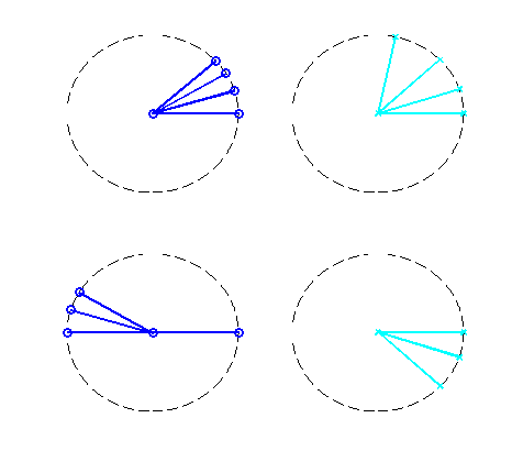
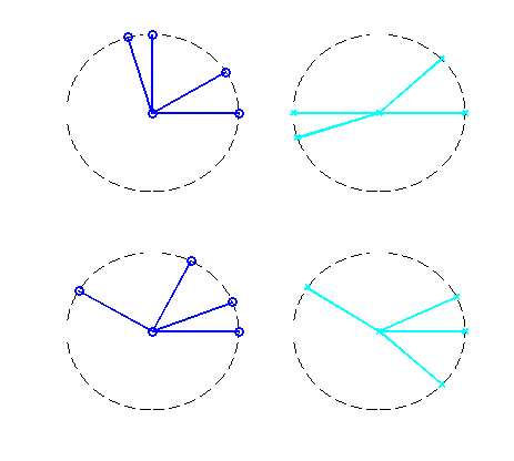
We make the following observation about the first alternative of Lemma 2.8. If $\{A_{k}\}_{k=1}^{M}\subset\mathbb{R}^{N}$ represents the column vectors of $A$, then there exists of a vector $0\neq x=(x_{k})_{k=1}^{M}$ with $x_{k}\geq 0$ such that $Ax=0$ is equivalent to saying that

Without loss of generality we may assume that $\sum_{k=1}^{M}x_{k}=1$, in which case the condition is equivalent to $0$ being a convex combination of the column vectors of $A$. Thus, having a nontrivial nonnegative vector in the null space of $A$ is a statement about the convex hull of the columns of $A$.

Motivated by the geometric intuition we gained from the two-dimensional setting and to effectively use Farkas’s lemma, we introduce a few notions from convex geometry, especially the theory of convex polytopes, and we refer to [68, 80] for more details on these concepts. For a finite set $X=\{x_{i}\}_{k=1}^{M}\subset\mathbb{R}^{N}$, the polytope generated by $X$ is the convex hull of $X$, which is a compact convex subset of $\mathbb{R}^{N}$. In particular, we denote this set by $P_{X}$ (or $\operatorname{co}(X)$), and we have

The affine hull generated by $X$ is defined by

We have $\operatorname{co}(X)\subset\operatorname{aff}(X)$. The relative interior of the polytope $\operatorname{co}(X)$ denoted by $ri\operatorname{co}(X)$, is the interior of $\operatorname{co}(X)$ in the topology induced by $\operatorname{aff}(X)$. We have that $ri\operatorname{co}(X)\neq\emptyset$ as long as $\#X\geq 2$, and

The polyhedral cone generated by $X$ is the closed convex cone $C(X)$ defined by

The polar cone of $C(X)$ is the closed convex cone $C^{\circ}(X)$ defined by

The cone $C(X)$ is said to be pointed if $C(X)\cap(-C(X))=\{0\},$ and blunt if the linear space generated by $C(X)$ is $\mathbb{R}^{N}$, i.e., $\linspan C(X)=\mathbb{R}^{N}$.

Using Proposition 2.7, we see that $\Phi$ is ($m-$)scalable if there exists $\{\lambda_{k}\}_{k\in I}\subset[0,\infty)$ , $\#I=m$ such that

This is equivalent to saying that $0$ belongs to the polyhedral cone generated by $F(\Phi_{I})=\{F(\varphi_{k})\}_{k\in I}.$ Without loss of generality we can assume that $\sum_{k\in I}\lambda_{k}=1$ which implies that $0$ belongs to the polytope generated by $F(\Phi_{I})=\{F(\varphi_{k})\}_{k\in I}.$ Putting these observations together with Lemma 2.8 the following results were established in [53, theorem 3.9]. In the sequel, we shall denote by $[K]$ the set of integers $\{1,2,\ldots,K\}$ where $K\in\mathbb{N}$.

The details of the proof of this result can be found in [53, Theorem 3.9]. We point out however, that the equivalence of (i) and (ii) follows from considering $\operatorname{co}(F(\Phi_{I}))$ which is the polytope in $\mathbb{R}^{N}$ generated by the vectors $\{F(\varphi_{k})\}_{k\in I}$.

References

- [1] S. T. Ali, J. P. Antoine, and J. P. Gazeau, Continuous frames in Hilbert spaces, Ann. Physics, 222 (1993), 1–37.
- [2] L. Ambrosio, N. Gigli, G. Savaré, “Gradients Flows in Metric Spaces and in the Space of Probability Measures,” Lectures in Mathematics ETH Zürich. Birkhäuser Verlag, Basel 2005.
- [3] W. Bajwa, R. Calderbank, D. G. Mixon, Two are better than one: fundamental parameters of frame coherence, Appl. Comput. Harmon. Anal., 33 (2012), no. 1, 58�78.
- [4] K. Ball, Ellipsoids of maximal volume in convex bodies, Geom. Dedicata 41 (1992), no. 2, 241–250.
- [5] K. Ball, An elementary introduction to modern convex geometry, Flavors of geometry, 1–58, Math. Sci. Res. Inst. Publ., 31, Cambridge Univ. Press, Cambridge, 1997.
- [6] V. Balakrishnan and S. Boyd, Existence and Uniqueness of Optimal Matrix Scalings, SIAM J. Matrix Anal. Appl., 16 (1995), no. 1, 29–39.
- [7] J. J. Benedetto, M. Fickus, Finite normalized tight frames, Adv. Comput. Math., 18 (2003), no. 2–4, 357–385.
- [8] J. J. Benedetto, J. D. Kolesar, Geometric properties of Grassmannian frames for and , EURASIP J. Applied Signal Processing, 2006, pp. 1–17.
- [9] M. Benzi, Preconditioning techniques for large linear systems: a survey, J. Comput. Phys., 182 (2002), no. 2, 418–477.
- [10] G. Björck, Distributions of positive mass, which maximize a certain generalized energy integral, Arkiv für Matematik, 3 (1955), 255–269.
- [11] J. Bourgain,On high-dimensional maximal functions associated to convex bodies, Amer. J. Math., 108 (1986), no. 6, 1467–1476.
- [12] J. Cahill, M. Fickus, D. G. Mixon, M. J. Poteet, and N. Strawn, Constructing finite frames of a given spectrum and set of lengths, Appl. Comput. Harmon. Anal., 35 (2013), no., 1, 52–73.
- [13] J. Cahill, N. Strawn, Algebraic geometry and finite frames, in “Finite frames”, Applied and Numerical Harmonic Analysis, (2013), 141–170, Eds: P. Casazza and G. Kutyniok, Birkhaüser.
- [14] J. Cahill and X. Chen, A note on scalable frames, Proceedings of SampTA 2013.
- [15] P. G. Casazza and G. Kutyniok, “Finite Frame Theory,” Eds., Birkhaüser, Boston, 2012.
- [16] P. G. Casazza, M. Fickus, J. Kovačević, M. Leon, and J. Tremain, A physical interpretation of tight frames, Harmonic analysis and applications, 51–76, Appl. Numer. Harmon. Anal., Birkhäuser Boston, Boston, MA, 2006.
- [17] P. G. Casazza, M. Fickus, and D. G. Mixon, Auto-tuning unit norm frames, Appl. Comput. Harmon. Anal., 32 (2012), no. 1, 1–15.
- [18] P. G. Casazza, M. Fickus, D. G. Mixon, Y. Wang, and Z. Zhou, Constructing tight fusion frames, Appl. Comput. Harmon. Anal. 30 (2011), no. 2, 175–187.
- [19] P. Casazza, A. Heinecke, K. Kornelson, Y. Wang, and Z. Zhou, Necessary and sufficient conditions to perform Spectral Tetris, Linear Algebra Appl., 438 (2013), no. 5, 2239–2255.
- [20] P. G. Casazza and J. Kovačević, Equal-norm tight frames with erasures, Frames, Adv. Comput. Math., 18 (2003), no. 2-4, 387–430.
- [21] A. Z. -Y. Chan, M. S. Copenhaver, S. K. Narayan, L. Stokols, and A. Theobold, On structural decompositions of finite frames, arXiv:1411.6138, (2014).
- [22] X. Chen, G. Kutyniok, K. A. Okoudjou, F. Philipp, and R. Wang, Measures of scalability, IEEE Trans. Inf. Theory, 61 (2015), no. 8, 4410–4423.
- [23] C. A. Clark and K. A. Okoudjou, On Optimal Frame Conditioners, arXiv:1501.06494, (2015).
- [24] H. Cohn and A. Kumar, Universally optimal distribution of points on spheres, J. Amer. Math. Soc., 20 (2007), no. 1, 99–148.
- [25] M. S. Copenhaver, Y. H. Kim, C. Logan, K. Mayfield, S. K. Narayan, and J. Sheperd, Diagram vectors and tight frame scaling in finite dimensions, Operators and Matrices, 8, no.1 (2014), 73 – 88.
- [26] P. Delsarte, J. M. Goethals, and J. J. Seidel, Spherical codes and designs, Geom. Dedicata, 6 (1997), 363–388.
- [27] D. Donoho, M. Elad, Optimally sparse representation in general (nonorthogonal) dictionaries via minimization, Proc. Natl. Acad. Sci. USA 100 (2003), no. 5, 2197–2202
- [28] M. Elad and A. M. Bruckstein, A generalized uncertainty principle and sparse representation in pairs of bases, IEEE Trans. Inform. Theory, vol. 48, pp. 2558–2567, Sept. 2002.
- [29] M. Ehler and K. A. Okoudjou, Minimization of the probabilistic frame potential, J. Statist. Plann. Inference, 142 (2012), no. 3, 645–-659.
- [30] M. Ehler, Random tight frames, J. Fourier Anal. Appl., 32 (2012), no. 1, 1–15.
- [31] M. Ehler and J. Galanis, Frame theory in directional statistics, Stat. Probabil. Lett. 81 (2011), no. 8, 1046–1051.
- [32] M. Ehler and K. A. Okoudjou, Probabilistic frames: An overview , in: “Finite Frames,” Applied and Numerical Harmonic Analysis, (2013), 415–436, Eds: P. Casazza and G. Kutyniok, Birkhaüser.
- [33] M. Fickus, B. D. Johnson, K. Kornelson, and K. A. Okoudjou, Convolutional frames and the frame potential, Appl. Comput. Harmon. Anal., 19 (2005), no. 1, 77–91.
- [34] M. Fickus, D. G. Mixon, M. J. Poteet, N. Strawn, Constructing all self-adjoint matrices with prescribed spectrum and diagonal, Adv. Comput. Math., 39 (2013), no. 3–4, 585–609.
- [35] M. Fornasier and H. Rauhut, Continuous frames, function spaces, and the discretization problem, J. Fourier Anal. Appl., 11 (2005), no. 3, 245–287.
- [36] G. E. Forsythe and E. G. Straus, On best conditioned matrices, Proc. Amer. Math. Soc. 6 (1955), 340–345.
- [37] A. A. Giannopoulos, V. D. Milman, Extremal problems and isotropic positions of convex bodies, Israel J. Math. 117 (2000), 29–60.
- [38] A. C. Gilbert, M. Muthukrishnan, and M. J. Strauss, Approximation of functions over redundant dictionaries using coherence, in Proc. 14th Annu. ACM-SIAM Symp. Discrete Algorithms, Baltimore, MD, Jan. 2003, pp. 243–252.
- [39] V. K. Goyal, M. Vetterli, and N. T. Thao, Quantized overcomplete expansions in : analysis, synthesis, and algorithms, IEEE Trans. Inform. Theory 44 (1998), no. 1, 16–31.
- [40] O. Güler, Foundations of Optimization, Graduate Texts in Mathematics, 258 Springer, New York, 2010.
- [41] D. Han, K. Kornelson, D. Larson, and E. Weber, Frames for Undergraduates, American Mathematical Society, Providence, RI, 2007.
- [42] C. Heil, What is a frame?, Notices Amer. Math. Soc. 60 (2013), no. 6, 748–750.
- [43] N. Higham, “Accuracy and Stability of Numerical Algorithms,” Second edition. Society for Industrial and Applied Mathematics (SIAM), Philadelphia, PA, 2002.
- [44] Y. Hur and K. A. Okoudjou, Scaling Laplacian Pyramids, SIAM. J. Matrix Anal. Appl., 36(1), 348–365.
- [45] F. John, Extremum problems with inequalities as subsidiary conditions, Studies and Essays Presented to R. Courant on his Birthday, January 8, 1948, 187–204. Interscience Publishers, Inc., New York, N. Y., 1948.
- [46] B. D. Johnson, and K. A. Okoudjou, Frame potential and finite Abelian groups, Contemporary Math., AMS, Vol. 464 (2008), 137–148.
- [47] C. R. Johnson, and R. Reams, Scaling of symmetric matrices by positive diagonal congruence, Linear Multilinear Algebra 57 (2009), no. 2, 123–140.
- [48] L. Khachiyan, and B. Kalantari, Diagonal matrix scaling and linear programming, SIAM J. Optim. 2 (1992), no. 4, 668–672.
- [49] B. Klartag and G. Kozma, On the hyperplane conjecture for random convex sets, Israel J. Math., 170 (2009), 253–268.
- [50] J. Kovacevic and A. Chebira, Life Beyond Bases: The Advent of Frames (Part I), Signal Processing Magazine, IEEE Volume 24, Issue 4, July 2007, 86–104
- [51] J. Kovacevic and A. Chebira, Life Beyond Bases: The Advent of Frames (Part II), Signal Processing Magazine, IEEE Volume 24, Issue 5, Sept. 2007, 115–125.
- [52] G. Kutyniok, K. A. Okoudjou, F. Philipp, and K. E. Tuley, Scalable frames, Linear Algebra Appl., 438 (2013) 2225–2238.
- [53] G. Kutyniok, K. A. Okoudjou, and F. Philipp, Scalable frames and convex geometry, Contemp. Math. 626 (2014), 19–32.
- [54] G. Kutyniok, K. A. Okoudjou, and F. Philipp, Perfect preconditioning of frames by a diagonal operator, Proceedings of the 10th International Conference on Sampling Theory and Applications pp. 85-88.
- [55] J. Lemvig, C. Miller, and K. A. Okoudjou, Prime tight frames, Adv. Comput. Math., 40 (2014), no. 2, 315–334.
- [56] E. Levina, P. Bickel, The Earth Mover’s distance is the Mallows distance: some insights from statistics, Eighth IEEE International Conference on Computer Vision, 2 (2001), 251–256.
- [57] E. Levina, R. Vershynin, Partial estimation of covariance matrices, Probability Theory and Related Fields 153 (2012), 405–419.
- [58] K. V. Mardia, E. P. Jupp, “Directional Statistics,” John Wiley & Sons, Wiley Series in Probability and Statistics, 2008.
- [59] P. Massey and M. Ruiz, Minimization of convex functionals over frame operators, Adv. Comput. Math., 32 (2010), no. 2, 1302–1316.
- [60] J. Matoušek, Lectures on Discrete Geometry, Graduate Texts in Mathematics, 212 (2002), Springer-Verlag, New York.
- [61] V. Milman, A. Pajor, Isotropic position and inertia ellipsoids and zonoids of the unit ball of normed dimensional space, In Geometric aspects of functional analysis, Lecture Notes in Math., 64–104, Springer, Berlin, 1987-88.
- [62] O. Oktay. “ Frame quantization theory and equiangular tight frames,” Ph. D thesis, University of Maryland (2007).
- [63] J. M. Renes, R. Blume-Kohout, A. J. Scott, and C. Caves, Symmetric informationally complete quantum measurements, J. Math. Phys. 45 (2004), no. 6, 2171–2180.
- [64] M. Rudelson, Approximate John’s decompositions, Geometric aspects of functional analysis (Israel, 1992–1994), 245–249, Oper. Theory Adv. Appl., 77, Birkhäuser, Basel, 1995.
- [65] M. Rudelson, Contact points of convex bodies, Israel J. Math. 101 (1997), 93–124.
- [66] J. J. Seidel, Definitions for spherical designs, J. Statist. Plann. Inference, 95 (2001), no. 1–2, 307–313.
- [67] J. Stoer and C. Witzgall, Transformations by diagonal matrices in a normed space, Numer. Math. 4 (1962) 158–171.
- [68] J. Stoer, and C. Witzgall, Convexity and optimization in finite dimensions I., Die Grundlehren der mathematischen Wissenschaften, Band 163, Springer-Verlag, New York-Berlin, 1970.
- [69] N. Strawn, Finite frame varieties: nonsingular points, tangent spaces, and explicit local parameterizations, J. Fourier Anal. Appl., 17 (2011), no. 5, 821–853.
- [70] N. Strawn, Optimization over finite frame varieties and structured dictionary design, Appl. Comput. Harmon. Anal., 32 (2012), no. 3, 413–434.
- [71] T. Strohmer and R. W. Heath Jr.,Grassmannian frames with applications to coding and communication, Appl. Comput. Harmon. Anal., 14 (2003), no. 3, 257–275.
- [72] N. Tomczak-Jaegermann, Banach-Mazur Distances and Finite-Dimensional Operator Ideals, Pitman Monographs and Surveys in Pure and Applied Mathematics, 38 Longman Scientific Technical, Harlow; copublished in the United States with John Wiley Sons, Inc., New York, 1989.
- [73] L. F. Tóth, Distribution of points in the elliptical plane, Acta Mathematica Academiae Scientiarum Hungaricae, vol. 16 (1965), 437–440.
- [74] J. A. Tropp, Greed is good: algorithmic results for sparse approximation, IEEE Trans. Inform. Theory 50 (2004), no. 10, 2231–2242.
- [75] B. Venkov, “Réseaux et designs sphériques,” In Réseaux Euclidiens, Designs Sphériques et Formes Modulaires, Monogr. Enseign. Math., 37, Enseignement Math., 10–86, Gèneve, 2001.
- [76] R. Vershynin, John’s decompositions: selecting a large part, Israel Journal of Mathematics 122 (2001), 253–277.
- [77] R. Vershynin, How close is the sample covariance matrix to the actual covariance matrix? Journal of Theoretical Probability 25 (2012), 655–686.
- [78] C. Villani, “Optimal transport: Old and new,” Grundlehren der Mathematischen Wissenschaften, 338, Springer-Verlag, Berlin 2009.
- [79] S. Waldron, Generalized Welch bound equality sequences are tight frames, IEEE Trans. Inform. Theory 49 (2003), no. 9, 2307–2309.
- [80] R. Webster, “Convexity,” Oxford Science Publications. The Clarendon Press, Oxford University Press, New York, 1994.
- [81] L. R. Welch, Lower bounds on the maximum cross correlation of signals, IEEE Trans. Inform. Theory, vol. IT-20 (1974), 397–399.
- [82] C. G. Wickman, “An optimal transport approach to some problems in frame theory,” Thesis (Ph.D.) University of Maryland, College Park, 2014, 129 pp.
- [83] C. Wickman Lau and K. A. Okoudjou, Scalable probabilistic frames, arXiv:1501.07321 (2015).
- [84] G. Zauner, “Quantum designs—Foundations of non-commutative theory of designs” (in German), Ph.D. thesis, University of Vienna, 1999. Available online at http://www.math.univie.ac.at/neum/papers.html.
- [85] MAPS-REU: http://www-math.umd.edu/maps-reu.html