A Functional and its Relaxation for Joint Motion Estimation and Image Sequence Recovery
Abstract
The estimation of motion in an image sequence is a fundamental task in image processing. Frequently, the image sequence is corrupted by noise and one simultaneously asks for the underlying motion field and a restored sequence. In smoothly shaded regions of the restored image sequence the brightness constancy assumption along motion paths leads to a pointwise differential condition on the motion field. At object boundaries which are edge discontinuities both for the image intensity and for the motion field this condition is no longer well defined. In this paper a total-variation type functional is discussed for joint image restoration and motion estimation. This functional turns out not to be lower semicontinuous, and in particular fine-scale oscillations may appear around edges. By the general theory of vector valued functionals its relaxation leads to the appearance of a singular part of the energy density, which can be determined by the solution of a local minimization problem at edges. Based on bounds for the singular part of the energy and under appropriate assumptions on the local intensity variation one can exclude the existence of microstructures and obtain a model well-suited for simultaneous image restoration and motion estimation. Indeed, the relaxed model incorporates a generalized variational formulation of the brightness constancy assumption. The analytical findings are related to ambiguity problems in motion estimation such as the proper distinction between foreground and background motion at object edges.
1 Introduction
In computer vision, the accurate computation of motion fields in image sequences—frequently called optimal flow estimation—is a long standing problem, which has been addressed extensively. For a general overview on optical flow estimation we refer to the survey by Fleet and Weiss [22]. We consider an image sequence given via a grey value map
on a space time domain , where is a bounded Lipschitz domain in for . To begin with, we suppose that motion is reflected by the image sequence and that image points move according to a velocity field . Hence, constancy of grey values along motion trajectories with leads to the transport equation
| (1.1) |
as a constraint equation for the unknown velocity field . This constraint equation is generally known as the brightness constancy constraint and for the space time motion field it can be rewritten as . Here and in what follows denotes the space time gradient. This condition gives us pointwise one constraint for unknown velocity components. Indeed, only the component of the velocity orthogonal to isolines of the grey value can be computed from equation (1.1), which leads to an illposed problem known as the aperture problem. Nagel and Otte [37] and Tristanelli [47] suggested to consider second derivatives, i.e. along motion trajectories leads to so that, if is invertible, can be computed. Similarly, in more geometric terms the motion field can be described via temporal variations of the shape operator on level sets as proposed by Guichard [26]. Since second derivatives are involved, these pointwise approaches are vulnerable to noise and hence of difficult practical usability. Based on the assumption that the image intensity varies on a finer scale than , one might assume to be locally constant and accumulate locally different constraint equations to estimate . This dates back to the early work by Lucas and Kanade [34, 49] or the structure tensor approach [8], which minimizes the local energy functional for a local window function .
This paper aims at consistently treating the general case with basically two different types of representations of motion in image sequences:
- -
mostly smooth motion visible via spatial variations of object shading and texture and their transport in time,
- -
motion represented by moving object edges, frequently characterized by discontinuities in the motion velocity apparent at edges of moving objects.
The local approaches mentioned above are able to estimate the first type of motion and offer relatively high robustness with respect to noise but in general they do not lead to dense flow fields and fail to identify motion information concentrated on edges. Global variational approaches were initiated by the work of Horn and Schunck [28]. They considered minimizers of the energy functional implicitly assuming the optical flow field to be smooth. A rigorous numerical analysis for a finite difference discretization of the Horn–Schunck approach was performed by Le Tarnec et al. [33]. Nagel and Enkelmann [36] proposed to use an anisotropic regularization term with a smaller penalization for variations of in normal direction across edges. With a focus on real world applications, Weickert et al. [49] proposed a combination of local flow estimation and global variational techniques to combine the benefits of robustness and dense field representation, respectively. For a detailed analysis of the occlusion problem associated with the estimation of object motion we refer to the joint approach for motion estimation and segmentation by Kanglin and Lorenz [30]. Ito [29] suggested to treat the optical flow estimation in terms of an optimal control formulation. Brune et al. [12] used the optimal control paradigm to estimate intensity and motion edges in image sequences.
Before discussing total variation type approaches for motion estimation —to which our method belongs— we
investigate a basic but already characteristic optical flow problem.
A simple model problem.
Suppose an object with a shading or texture intensity map is moving with spatially constant velocity on a background with shading and texture intensity map , which is itself moving with constant velocity . Thus, the observed image sequence is given by
| (1.2) |
where denotes the characteristic function of the object domain .
Trying to retrieve the object and the two velocities from the
image sequence one observes the following:
- (i)
If both image intensities and are constant the role of foreground and background can be flipped, i.e. either the object or its complement is moving with speed , whereas the background velocity obviously cannot be determined.
- (ii)
If both shading or texture intensity maps and are smooth and locally allow the computation of and from (1.1), the decision on foreground and background is associated with the consistency of one of the velocities with the motion of the interface. Thereby, consistency is expressed in terms of the singular counterpart of (1.1), where and denotes the space time normal on the interface, which coincides with the jump set of the image function from (1.2).
- (iii)
If neither nor is consistent with the motion of the jump set then the object is undergoing a more complex evolution than just a rigid motion, e.g., growth or shrinkage.
In the general case, beyond this simple model problem, at each point on the jump set of the space time intensity map one should compare the values of the velocity and on the two sides with the space time interface normal on to decide on the actual local motion pattern. Hence, we are interested in a variational approach which explicitly incorporates this local consistency test, where the motion data and on the two sides are determined either via local shading or texture data or from a global relaxation principle taking into account far field motion data.
The space of functions of bounded variation () allows to describe configurations with singularities of codimension one, i.e. edge-type jump sets. Total variation regularization was first introduced in image processing by Rudin, Osher, and Fatemi [45]. Cohen [15] proposed to replace the usual quadratic regularization in the above motion estimation approaches by a type regularization . A more general convex regularizer with linear growth was investigated by Schnörr and Weickert [50]. A broader comparison of different regularization techniques in imaging and a discussion of suitable quasi-convex functionals was given by Hinterberger et al. [27]. In particular they considered a - approximation of type functionals. Papenberg et al. [40] investigated a regularization of the motion field and an optical flow constraint involving higher order gradients. In their pioneering paper Chambolle and Pock [14] suggested a duality approach for nonsmooth convex optimization problems in and discussed as one application the motion estimation problem. An improvement of the original ansatz was suggested by Wedel et al. [48] and an efficient implementation of this primal dual optimization approach to optical flow estimation was presented recently by Sánchez et al. [46].
The approach by Aubert and Kornprobst [6] is closely related to ours. They considered for the energy functional
| (1.3) |
extended to the space of velocity fields of bounded variation, where is a fixed image intensity map in and a function with linear growth. They discussed the following fundamental problem. On the jump set of , representing the space time edge surfaces, the singular part of the gradient is only a Radon measure and in the generic case of moving objects one expects a significant overlap of with the jump set of the motion field . Thus, it is unclear how to define . This is indeed a recasting of the above observation (ii) in the context of the theory of functions with bounded variation. Aubert and Kornprobst considered a locally averaged evaluation of the motion field, and they finally studied the relaxation of the above functional in . In the case of Lipschitz continuous image sequences, Aubert et al. [5] considered the numerical approximation of the above total variation functional based on a duality approach and a suitable approximation of with a sequence of functionals of quadratic growth.
Frequently the image sequence is corrupted by noise that one wishes to remove. On the theoretical side, we cannot assume that the input image intensity is already in . We study here a approach for the joint reconstruction of non smooth space time intensity maps and the underlying non smooth optical flow fields . It differs from the ansatz by Aubert and Kornprobst [6] in that here both fields are reconstructed simultaneously. We investigate in particular the relation to the above-discussed fundamental observations (i)—(iii) on motion estimation and show that the approach naturally incorporates a local analysis of the motion pattern in the vicinity of the jump set . Depending on the data, minimizing sequences may develop undesirable small-scale oscillations around interfaces. Analytically this means that the functional is not lower semicontinuous. The theory of relaxation permits to replace the functional by its lower semicontinuous envelope, thereby eliminating the fine-scale oscillations from the kinematics, but still incorporating their averaged effect in the energetics. The key technical ingredient we use here is a general result on the relaxation of variational problems on vector-valued functions by Müller and Fonseca [23] and earlier work on relaxation on functions by Ambrosio and Dal Maso [4] and Aviles and Giga [7]. It leads to the relaxed functional presented in (2.3) below. The ambiguity close to the jump set is then resolved by minimizing locally a suitable microscopic problem, which in turn leads to a selection of the relevant local motion pattern, see (2.4) below. Using upper and lower bounds on the relaxed energy we can show that under suitable (implicit) assumptions on the image intensity map and the motion field such microscopic oscillations can be ruled out.
The advantages of the joint estimation of intensity and motion field are the following:
- -
A reliable segmentation of moving objects via the non smooth intensity map helps to estimate their motion.
- -
Given the motion field, the brightness constancy assumption along motion paths significantly improves the denoising of the image sequence or even the restoration of missing frames.
- -
Reliable motion detection also poses an important cue for object detection and recognition.
Thus, joint approaches which simultaneously estimate the motion field, segment objects and denoise the image sequence are particularly appealing. Advances in this direction were investigated in [51, 39, 13, 35, 41]. A first approach which relates optical flow estimation to Mumford–Shah image segmentation was presented by Nesi [38]. Cremers and Soatto [17, 18, 19] gave an extension of the Mumford-Shah functional from intensity segmentation to motion based segmentation in terms of a probabilistic framework.
Rathi et al. investigated active contours for joint segmentation and optical flow extraction [42]. Brox et al. [11] presented a Chan-Vese type model for piecewise smooth motion extraction. For given fixed image data the decomposition of image sequences into regions of homogeneous motion is encoded in a set of level set functions and the regularity of the motion fields in these distinct regions is controlled by a total variation functional. Indeed, Kornprobst et al. [31] already studied a joint approach for the segmentation of moving objects in front of a still background and the computation of the motion velocities.
The paper is organized as follows. In Section 2 we introduce the variational approach via the definition of a suitable energy on space time intensity maps and motion fields and retrieve the general relaxation result for this type of energies. The functional we propose to use is given in (2.3-2.4). On the jump sets of and the integrand of the relaxed functional involves a microscopic variational problem. The main contribution of this paper is to establish bounds for this microscopic energy and to give sufficient conditions for the non existence of microscopic oscillations. In Section 3 we discuss the consequences of our results for optical flow estimation. Then, in Section 4 we present the proofs of the results discussed in Section 2.
2 Variational approach and relaxation results
In this section we derive a joint functional for the restoration of a space time image sequence and the estimation of the underlying motion field. We start by fixing some notation. We denote by the image domain, a bounded Lipschitz-domain in with , and by the associated space time domain. For a spatial vector we write , while time-space vectors are denoted by with being the time coordinate. Correspondingly, the space time gradient reads as . We use for the Euclidean norm including all matrix spaces. We use standard notation and with for Lebesgue and Sobolev spaces, respectively. By the fundamental decomposition result [3, 21] the derivative of a function of bounded variation can be written as
where for and . Here is the jump set of , is the jump, are the approximate limits on , is the measure theoretic normal to and is the Cantor part of the measure , orthogonal to both and . The jump part of is denoted by .
Let represent the input data, a given grey valued image sequence, with . Our aim is to determine a restored image sequence and an underlying motion field . Throughout this paper we use the shortcut notation for the space time motion field. Since we expect that both the reconstructed image sequence and the reconstructed image velocities will jump on the boundaries of reconstructed moving objects, which are codimension surfaces in space time, we consider as the suitable space for intensity maps and as the suitable space for velocity fields.
We start by defining a functional measuring the quality of the restoration and the motion extraction for an image sequence and a motion field . The actual functional on will then be defined via relaxation. For fixed and we consider the following energy integrand
and define for a general Lipschitz domain the energy
| (2.1) |
This energy is then complemented with a fitting term with respect to the given image sequence to obtain the functional
The energy is finite for and with and measuring the regularity of the motion field and the image sequence , respectively. Furthermore,
quantifies the agreement of the pair with the brightness constancy constraint (1.1). We remark that for general input image sequences bounds on the energy do not imply a priori bounds on the motion field in , for example in the case that is spatially uniform. The constraint on has been included to avoid this technical difficulty.
At this point we are ready to define the actual functional of interest for as the relaxation of the functional with respect to convergence in :
| (2.2) |
As already mentioned in the introduction in the generic case of optical flow applications the jump set of the motion field (the union of boundaries of moving objects) is a subset of the jump set of the image intensity (the union of all image edges). Hence, is expected to jump on a subset of the support of the jump part of the measure , so that the term is ill-defined. A proper understanding of this term requires to select locally a microscopic profile for and and includes —but will not be restricted to— the proper choice between or for the pointwise value for in the term and thus the local selection between foreground and background (cf. the consistency issue (ii) in the simple model problem in Section 1). In fact, the theory of relaxation for problems with linear growth is more complex than the one with -growth, [20], because of the singular part of the gradient in the limit. Relaxation and lower semicontinuity with a convex integrand depending only on the gradient field were already obtained in the 60s [25, 43], the general case, with dependence of the integrand also on and was investigated in the early 90s [4, 7]. Here, we use the more general result by Fonseca and Müller in [23], which also includes the case of quasiconvex integrands, as the starting point of our investigation. Successive developments include [10, 9, 24, 32, 44].
These results show that the relaxation of with respect to the -topology, as defined in (2.2), is finite on the domain
and it equals
| (2.3) |
Since is one-homogeneous and convex in the second and third arguments, coincides with its regression function and the third term in (2.3) should be interpreted as
The key nonconvexity arises from the dependence of on the first variable in the jump part. Thereby, the function depending on the approximate limits and of and the measure theoretic normal on the jump set is the solution of a local minimizing problem in which the energy on the jump is optimized with respect to all possible microstructures. Precisely,
| (2.4) |
where is the rotated cube
with denoting an orthonormal basis of , and is the set of -functions which have traces on the two sides of normal to and are periodic in the - directions,
We remark that the term is continuous in with respect to the weak convergence in , since we chose . Furthermore, both and are coercive in , in the sense that for any given and for any sequence with bounded, the sequence of norms of and are also bounded. Therefore the above representation of the relaxation follows immediately from the more general statement of Fonseca and Müller [23, Theorem 2.16] and existence of minimizers for the relaxed functional follows easily by the direct method of the calculus of variations.
A practical usage of the functional requires knowledge of the effective surface energy , much as in the case of relaxation on spaces one needs to determine the quasiconvex envelope of the integrand [20]. A numerical computation is in principle feasible via the minimization in (2.4), but it is nevertheless useful to extract analytical information on as far as possible. In what follows we give lower and upper bounds for the singular term and compute it explicitly in special cases. Thereby, we show that the model favors locally simple (i.e. planar) profiles in the microscopic problem (2.4) under reasonable assumptions from the viewpoint of the practical optical flow application. This renders the functional well-suited for joint image sequence restoration and motion extraction. A detailed discussion of the consequences of the bounds for is postponed to Section 3.
Theorem 2.1.
Given , and for the following statements hold:
- (i)
If then
- (ii)
For and one has , where
with ,
- (iii)
For general one has , where
where and the minimum is taken over and the set of vectors and , subject to .
The proof is given in Section 4.3.
The upper bounds in Theorem 2.1 are based on suitable choices for the optimal microscopic solution , of (2.4). If the profile of these microscopic solutions depend only on , we call it simple. There are in particular two types of simple profiles when solving (2.4) for given data , , and . In the case we define the following piecewise constant functions and :
| (2.5) |
where is chosen in the line segment such that for . For suitable approximations in such as those obtained by convolution , we have that
| (2.6) |
where and . This profile corresponds to a microscopic consistency with a interpretation of the brightness constancy constraint (1.1). In the other case consistency of a simple and optimal microscopic profile is out of reach. Let us assume that . Then a feasible, simple profile for the minimization of is given by
Indeed, again using the same ansatz for the approximation as above, one obtains
| (2.7) |
Figure 1 shows sketches of the simple profiles in both cases. In the next theorem we establish sufficient conditions for the existence of minimizing profiles which are simple.
Theorem 2.2.
Let , and , then we have the following.
- (i)
If then the optimal profile for is simple and
- (ii)
If , , and then the minimizing profile for is simple and
(2.8) - (iii)
If , and then the minimizing profile for is simple and given by (2.8) .
- (iv)
If the profile is simple, then
3 Consequences for the motion estimation
In this section we discuss the practical implications of Theorem 2.2 on the actual optical flow estimation based on the proposed variational approach for the joint image sequence restoration and motion extraction. We will analyze implicit conditions on the approximate limits of and at jump sets under which the singular energy density defined in (2.4) is simple and there is no relevant microscopic scale arising in the variational model. Furthermore, we will give an example where microstructures actually appear and thus the singular energy density is not simple. As the only interesting cases appear where , in this section we always assume that .
We start observing that the condition for simple profiles in one space dimension in Theorem 2.2 (ii) includes in particular the case
| (3.1) |
as well as the case
| (3.2) |
Hence, for moderate speed of the intensity interface (associated with large ) and either moderate difference of the estimated motion on both sides of the interface or moderate intensity variation the condition in Theorem 2.2 (ii) is fulfilled (in particular for ( and ) or ( and )). For the case the condition in Theorem 2.2 (iii) can be rephrased as
Thus, if is small, this condition is fulfilled for a moderate speed of the intensity interface (associated with large spatial component of ) and for a direction of the jump with a significant component pointing in direction of the spatial interface normal .
In the practical application the velocities on the two sides of the discontinuity and are determined within the variational setting by shading or texture information on both sides of the edge set . Then, the singular energy density is associated with the proper identification of the type of object motion as described for the simple model problem in Section 1, in particular the decision on foreground or background and the identification of additional erosion or dilation. As we will see below, for simple the minimization of the joint functional is able to decide on the motion pattern. In the case that is not simple and that microstructures appear the variational model seems not to appropriately reflect the scope of possible motion patterns. On the other hand, under the reasonable implicit assumption that the data fulfills one of the conditions under which the singular energy density is simple the joint variational approach actually renders the coupled restoration and motion estimation problem meaningful including the proper identification of the local motion pattern at object edges.
In what follows we study the different local motion pattern at some point and the associated singular energy density in more detail.
Consistent interface motion.
Let us suppose that a light object with image intensity is moving with a speed on a dark background with speed and image intensity () (cf. left sketch in Fig. 2). The consistency of the interface motion of the space time edge set with the object motion is expressed in terms of the brightness constancy assumption at the point with denoting the space time normal on , i.e. . In this case Theorem 2.2 (i) applies and . Microscopically this is realized by the profile sketched in Fig. 1 (left) with . Due to noise the brightness constancy assumptions might only be approximately fulfilled with . Then, Theorem 2.2 (ii) shows that we obtain the corresponding approximate singular energy density .
Non consistent interface motion.
Let us suppose that in the same configuration (cf. middle sketch in Fig. 2). Hence, neither the object motion nor the motion (currently classified as background) is consistent with the motion of the interface . Indeed, we observe an erosion of the interface. Let us assume that is the actual speed of the interface with for , then is the effective erosion velocity and is the associated footprint in the singular energy density , which is in agreement with the findings of Theorem 2.2 (ii). Obviously, the energy functional considers this classification as favorable compared to the one obtained via flipping object and background and classifying a foreground object with intensity moving with speed and dilation speed and larger footprint in the singular energy density . Microscopically this is realized by the profile sketched in Fig. 1 (right). If (cf. right sketch in Fig. 2) the variational approach favors the classification of a dilation process on the interface with velocity for the velocity on the line segment with and thus smallest possible singular energy density . The associated microscopic solution profile coincides with that sketched in Fig. 1 (left).
Objects and background with constant intensity.
Objects and background with constant intensity. If there is no shading or texture information, the estimation of motion velocities can solely be based on the observed motion of interfaces. Examplarily, let us suppose that objects are moving with constant velocities in front of a immobile background as sketched in Figure 3. Furthermore, let us explicitly rule out interface dilation and erosion. For such a configuration the singular energy density compares the different foreground and background configurations in the local depth ordering. For a fixed depth ordering of the objects the estimation of a velocity for each object is based on the minimization of with
where is the visible part of and , are the velocity and the intensity opposite , respectively. The estimation of the depth ordering via the variational approach is then performed by a comparison of the minimal total energy obtained for the set of all possible depth configurations (In Figure 3 the color of the interfaces shows which is the relevant velocity of the singular energy density for the minimal total energy). An estimation of the background speed is obviously not possible.
Appearance of microstructures.
By the above discussion it is clear that we have to deal with large relative velocities and jumps in the intensities. The key idea is to find a case where the upper bound in Theorem 2.1(ii) and (iii) is lower than the energy of simple profiles given in Theorem 2.2(iv).
We discuss first the case . Let and let be the upper bound given in Theorem 2.1(ii). We assume that
Then the energy of a simple profile in Theorem 2.2(iv) coincides with . Indeed, if is between and then and ; if is outside that interval then, letting be the projection of on the interval, and . This proves that the minimum is attained at .
Therefore it suffices to construct a situation where is not a minimizer of the upper bound function . For a vector chosen later and a small we compute, assuming and writing for brevity ,
where
Therefore it suffices to show that can be chosen so that .
We choose a large velocity , set , , , so that , , . We choose a normal which corresponds to motion with a velocity close to but not identical with the velocity . Precisely, for some we set . Then it is easy to see that . Finally we set , so that . It remains to show that and can be chosen so that . To do this we compute
which is negative if and are chosen sufficiently large (cf. Fig. 4). A detailed computation shows that and any will do. In the case , however, the Taylor series above is not admissible (since ) and the profile becomes simple again, in agreement with Theorem 2.2(i).
The construction can be easily generalized to the case . From the lower bound in Theorem 2.2(iv) we know that the best interfacial energy which can be attained using simple profiles is given by
for some . We choose as above a large velocity , set , , , , and pick a normal which corresponds to motion with velocity , namely, , for some . The optimal is also parallel to , and a short computation shows that it equals , so that
The one-dimensional result shows that there is such that . This result can be immediately embedded in the higher- dimensional setting by taking , , , , in the upper bound of Theorem 2.1(iii). Therefore the same values, and , will do.
We refer to Section 4.4 for a visualization of a more general microscopic pattern in the case .
Potential impact on the numerical implementation of the motion estimation model.
The model studied here has a built–in consistency with respect to the local shading or texture information and to the global geometry of moving and deforming objects in space–time, and is therefore attractive for concrete applications to imaging, based on an appropriate numerical implementation. The possible appearance of microstructures is, however, a very problematic feature of the model. If microstructure appears the usability of the model in imaging is questionable.
The analysis presented in this paper shows that microscopic patterns appear only if the motion velocity encoded in the edge set is relatively large and the motion data and encoded in the shading or the texture on both sides of the edge are substantially inconsistent with . Thus, in imaging applications the criteria for simple profiles stated in Theorem 2.2 and discussed at the beginning of this section mostly rule out the appearance of microstructures and indicate that a one-scale method should be appropriate in normal situations. The criteria in Theorem 2.2 can be used in a numerical algorithm as an a-posteriori test for the appropriateness of the one-scale model based on upscaled versions of , , , , and . If this test fails, it may be advisable to modify the the parameters , and , in ways which are suggested by the conditions in Theorem 2.2. Failure of the test, if one does not appropriately modify the parameters of the problem, leads to microscopic patterns. In particular, one would expect to observe oscillations in the single–scale numerical approximation of and in the vicinity of the edge set , with a length scale given by the spatial discretization. In fact, the constructions used in the proofs of the upper bounds could be used to set up a reduced microscopic model in a two–scale discretization approach, which would include a local optimization over a small set of parameters describing the microstructure. Numerical two-scale methods of this type are of theoretical interest, but in this concrete application they are of no practical relevance.
For a practical implementation of the single–scale model it is useful to observe that the functional is not jointly convex in and . However, is separately convex in and in and thus classical primal-dual methods can be applied in an alternating minimization scheme.
4 Proofs of the main results
In this Section we prove Theorem 2.1 and Theorem 2.2. We start by discussing the symmetries of the function and reformulating its definition on a different space of test functions in Section 4.1. Moreover, we prove classical subadditivity and convexity properties for . Then, in Section 4.2 we discuss explicit constructions which lead to upper bounds of for and prove a lower bound of for . Based on the ingredients of Section 4.1 the proofs of the theorems are then given in Section 4.3. Finally, in Section 4.4 we illustrate the possible microscopic patterns which might arise in critical regimes complementing the discussion in Section 3.
4.1 Preliminaries
In order to simplify the following discussion we first list the symmetries which obeys.
Lemma 4.1.
has the following symmetries:
-
,
-
,
-
,
-
.
Proof.
They all follow immediately from the definition. For the first equality replace by . For the second item replace by . For the third equality replace and by and . The last invariance is simply a relabeling of the boundary conditions. ∎
One key observation is that we can replace the set of functions in the definition of by a simpler class of functions. In particular, the function can be assumed to take only two values, and the velocity field can be assumed to be smooth. This allows to give a classical sense to the term . We stress that existence of minimizers is not expected in this restricted class, indeed functions of this class are later interpreted as microstructures.
Lemma 4.2.
In the definition of in (2.4) the set can be replaced by
Proof.
We prove the claim in three steps. If then one immediately obtains from which the result follows easily by standard density results. Hence we only need to deal with the case .
Step 1. First we show that , where
To prove the inequality, we choose and can assume that . We extend and periodically to and constantly in the -direction and define . Then a straightforward computation shows that
For we define where is a standard mollifier. Since is constant on and , the functions satisfy .
To prove convergence of the energy we first observe that by the general properties of mollification of Sobolev functions we immediately obtain and in and , respectively. The more subtle term is , where . Since we can estimate
The first term on the right hand side can be estimated by
For the second term we observe that pointwise a.e. and that
Hence by Lebesgue’s dominated convergence theorem we derive
Therefore
concludes the proof of the first step.
Step 2. We show that . Let , assume for definiteness that . The coarea formula yields
Indeed, the first term is standard, the second one follows easily from [3, (3.33) in Th. 3.40] approximating uniformly with piecewise constant vector fields.
Thus there exists such that
We define and . Then
where on the right hand side has to be interpreted as a measure. Since the function is smooth, it is in particular continuous on the jump set , hence the integral is well defined. Furthermore by the trace theorem fulfills the boundary conditions. Therefore and .
Step 3. We prove that . As in Step 1 we choose , extend both functions periodically, scale them to , and mollify (but not ) to obtain . For the same reasons as in Step 1 we have and
It remains to show that , where as usual . To see this, we deduce from for the Radon measure that (cf. [3, Prop. 3.7])
Furthermore,
converges to zero because is uniformly continuous on . Hence
which proves the claim. ∎
Next we give an iterated relaxation formula.
Lemma 4.3.
For we have
where for with being the normal to .
Proof.
Next we prove two more general properties, namely, subadditivity and convexity of the surface energy , which are well known for example in the setting of variational problems on partitions [1, 2]. We start with subadditivity and its main consequence in the present setting.
Lemma 4.4 (Subadditivity).
Let , , . Then:
- (i)
For any , one has
- (ii)
For any one has
Proof.
(i): For we define
Clearly in and for all . Since is lower semicontinuous, we obtain
which concludes the proof.
We next show that is convex in the last argument, after having been extended to a positively one-homogeneous function. This will be linked to the possible development of oscillations of the interface.
Lemma 4.5 (Convexity).
For given , we define by
The function is positively one-homogeneous and convex, in particular,
| (4.1) |
Proof.
Positive one-homogeneity is obvious from the definition. It implies , hence convexity is equivalent to subadditivity; therefore it suffices to prove the inequality (4.1). Furthermore, it suffices to consider the case that with and linearly independent (the case that and are parallel, including the case that one vanishes, is immediate).
By the scaling argument used in the proof of Lemma 4.3 it suffices to construct functions which are periodic in the directions orthogonal to and with whenever , for some . We shall first construct a curve that can be interpreted as the jump set of a function satisfying the boundary conditions. The curve will consist of two subsets, one has normal and measure , the other has normal and measure . To make this precise, we define , where is a 90-degree rotation in the plane spanned by and . We define
so that ends at , with . We set , choose such that is an orthonormal basis of , and define , see Fig. 5 (notation: ). This is a -dimensional surface, corresponding to the constant extension in the directions of the curve obtained joining alternatively copies of the segments and . In particular, has exactly two connected components; one of them, call it , contains and the other, call it , contains , where , see Fig. 5. We set . Then the normal to the jump set is on a set of measure , and correspondingly for . We define by rescaling , so that in . Therefore, dropping the arguments for brevity,
∎
4.2 Upper and lower bounds for
Proposition 4.6 (Construction for ).
Let and , . Then for any we have
where and .
Proof.
The result follows by Lemma 4.5 and Lemma 4.4(ii), taking once and once . For the sake of illustration we give here a self-contained, explicit construction.
We start by replicating the construction of Lemma 4.5. Again, we first construct a curve that will be interpreted as the jump set of a function satisfying the boundary conditions, and which consists of two subsets, with the normals and . Precisely, we define as in the proof of Lemma 4.5
so that ends at . We set and . Then has exactly two connected components and for sufficiently large one of them, call it , contains and the other, call it , contains , see Figure 5. We set . Then fulfills the desired boundary conditions.
Ideally the function should equal on , and on . As an approximation we construct a function as follows (cf. Figure 8). Precisely, for , we set
and . It is easy to see that . Let now , where is a mollification kernel. Then (cf. Figure 8) there exists a constant , such that
- (i)
on ; ,
- (ii)
,
- (iii)
on .
Thus and a straightforward computation shows that
Finally, we can take arbitrarily small, which establishes the claim.
Figure 8: The picture shows the construction of and . On the dark part takes the value , on the grey part the value . The brown line is the part of the jump set of parallel to (), the blue line represents the part of with normal parallel to (). The black line indicates up to smoothing the jump set of . As can be seen this is in terms of length and normal essentially the jump set of .
∎
In order to prove the lower bound in Theorem 2.1 (ii) we need the following truncation lemma. As it is frequently the case in truncation, this can only be done if the relevant field (the velocity here) is scalar, and the result is therefore restricted to .
Lemma 4.7 (Truncation for ).
Let and be such that . Let , and be defined as
If , then we have
| (4.2) |
where and .
Proof.
Let , and be the outer normal to on , so that . We want to estimate the term
Since vanishes on and it is periodic in the direction we have that (here is the outer normal to ), and the same on . Therefore by the Gauss-Green formula
Estimating and averaging over the two sides of we obtain
where we used that locally either and , or . This concludes the proof. ∎
At this point we present the key lower bound in the one dimensional case. The main idea is to reduce the energy to an integral on the jump set of and separate it into different parts, in order to show that the optimal curve has a structure similar to the one used for the construction in the upper bound and illustrated in Figure 5. For this we start from the reduction to intensity maps which are characteristic functions, done in Lemma 4.2, and the truncation of , discussed in Lemma 4.7. Then we show that we can consider also functions which take only two values, and use this to subdivide into two subsets, a strategy similar to the one used in [16, Lemma 4.5] to obtain the relaxation of a line-tension model for dislocations in crystals.
Proposition 4.8 (Lower bound for ).
Let , , be such that . Then where
Remark. If then the minimizer belongs to the segment and makes the last term vanish, the bound reduces to .
Proof.
By Lemma 4.1 we can assume without loss of generality that . Let . By Lemma 4.7 we may further assume that . We write for a set of finite perimeter. Using the abbreviation and for the outer normal to on we have as in the proof of Lemma 4.7 and
We estimate
This is the key estimate to establish the lower bound, and it is sharp if the three integrands have a constant orientation on the respective domains.
We observe that the quantity on the right-hand side depends only on the value of on . Indeed, since is periodic in the direction orthogonal to and ,
and the same on . We therefore define by
so that (we recall that is the time component, the space component)
Existence of a minimizer in follows immediately from the convexity of the functional . Even more, the functional is weakly continuous on , and therefore for any there is such that . This permits us to reduce to the situation where also the velocity takes only two values.
We split into two subsets depending on the value of :
and define
These quantities characterize the effective orientation of and , corresponding to the two normals in Proposition 4.6 and Lemma 4.5. Since is constant in each of the two subsets of , by convexity one could assume that is also constant on each of them, and then rearrange so that is composed of two segments. This illustrates the idea behind the energy bound, however it is not needed to conclude the proof.
It suffices indeed to separate the integrals in the definition of into a and a part, then a short computation gives
where . Since and by periodicity this gives
for all and , which concludes the proof. ∎
4.3 Proofs of Theorem 2.1 and 2.2
At first we prove a lower bound in the higher dimensional case.
Proposition 4.9 (Lower bound for ).
For let us define and with denoting the outer normal of on . Then
where
Proof.
Now we proceed with the proofs of the main theorems.
Proof of Theorem 2.1.
First we treat the case (i), where the optical flow constraint can be satisfied locally.
To prove the upper bound we first choose such that . The upper bound follows then from Lemma 4.4(ii), taking . For the sake of illustration we give also an explicit construction here. Let be a smooth monotone function such that , and . We set
| (4.3) |
and observe that . A simple computation shows that .
To prove the lower bound we choose and verify using convexity and periodicity
This concludes the proof of (i).
Proof of Theorem 2.2.
(ii): By Proposition 4.8 we have , where
We first show that if then is a minimizer of . Since is convex, it lies above its tangent, . Using for the last term we obtain
Using the fact that is positive we obtain
where
Since by assumption we have
therefore .
Recalling the upper bound we have , and since we conclude that in the case one has , with a simple profile since we have set in the construction of the upper bound. The same result still holds if , as a simple inspection of the lower bound shows.
Swapping with and using Lemma 4.1 we obtain that if then again with a simple profile. For the two assertions coincide. Since for our assumption is only satisfied in the trivial case and , we have shown that if and are nonzero and have the same sign the profile is simple and the interfacial energy is either or ; since they are both admissible the energy necessarily is the minimum of the two.
(iii): At first we observe that Lemma 4.4 (ii) implies that is an upper bound. Swapping with we can assume that and are strictly positive, swapping with we can assume that
From Proposition 4.9 we know that with
Notice that
As it suffices to show that has a minimum at . Since is convex this is the case if and only if is a subgradient at . It can be easily seen that the set of subgradients of at is
Hence if and only if
(we recall that we are using the Euclidean norm on ). Squaring the left hand side shows that this is equivalent to
which in turn is the same as
This holds since we are in the case and by assumption .
We finally prove (iv). The upper bound follows from Theorem 2.1(iii) with . To prove the lower bound, we observe that the construction in Lemma 4.2 does not modify the property of being one-dimensional, hence we can assume that are of the form , , for some set of finite perimeter and some function . Then, setting ,
With the assertion follows. ∎
4.4 Illustration of expected microstructures for

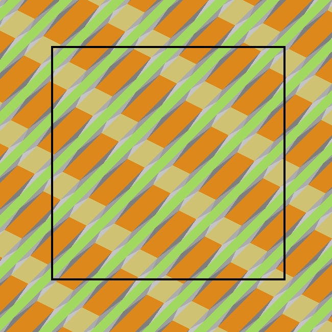
In the higher dimensional case () the upper bound in Theorem 2.1 (iii) refers to a set of vectors (). In the case the corresponding vectors and explicitly appear in a geometric construction of a microscopic pattern in the proof of Proposition 4.6. Using the convexity of the microscopic energy stated in Lemma 4.5 this explicit construction is not required in the proof of Theorem 2.1 (iii). Nevertheless, explicit microscopic patterns can be constructed, where the vectors are weighted normals with being the normal on a set of interface facets of total area . Figure 9 sketches for such a microscopic pattern with three weighted normals
where is a suitable rotation in . The resulting effective interface normal is the macroscopic normal on the jump set . The underlying pattern is based on nested lamination, i.e. a lamination pattern of facets perpendicular to and (plotted in light and dark orange) is altered with facets perpendicular to (plotted in green). To compensate the lack of rank- consistency a thin transition pattern is introduced in between (plotted in grey).
References
- [1] L. Ambrosio and A. Braides. Functionals defined on partitions in sets of finite perimeter. I. Integral representation and -convergence. J. Math. Pures Appl. (9), 69:285–305, 1990.
- [2] L. Ambrosio and A. Braides. Functionals defined on partitions in sets of finite perimeter. II. Semicontinuity, relaxation and homogenization. J. Math. Pures Appl. (9), 69:307–333, 1990.
- [3] L. Ambrosio, N. Fusco, and D. Pallara. Functions of bounded variation and free discontinuity problems. Oxford Mathematical Monographs. Oxford University Press, New York, 2000.
- [4] L. Ambrosio and G. Dal Maso. On the relaxation in of quasi-convex integrals. J. Funct. Anal., 109(1):76–97, 1992.
- [5] G. Aubert, R. Deriche, and P. Kornprobst. Computing optical flow via variational techniques. SIAM J. Appl. Math., 60:156–182, 1999.
- [6] G. Aubert and P. Kornprobst. A mathematical study of the relaxed optical flow problem in the space . Siam J. Math. Anal., 30:1282–1308, 1999.
- [7] P. Aviles and Y. Giga. Variational integrals on mappings of bounded variation and their lower semicontinuity. Arch. Rational Mech. Anal., 115(3):201–255, 1991.
- [8] J. Bigun and G. H. Granlund. Optical flow based on the inertia matrix of the frequency domain. In Proceedings from SSAB Symposium on Picture Processing : Lund University, Sweden, pages 132–135, 1988.
- [9] G. Bouchitté, I. Fonseca, G. Leoni, and L. Mascarenhas. A global method for relaxation in and . Arch. Ration. Mech. Anal., 165:187–242, 2002.
- [10] G. Bouchitté, I. Fonseca, and L. Mascarenhas. A global method for relaxation. Arch. Ration. Mech. Anal., 145:51–98, 1998.
- [11] T. Brox, A. Bruhn, and J. Weickert. Variational motion segmentation with level sets. In A. Pinz H. Bischof, A. Leonardis, editor, Computer Vision – ECCV 2006., volume 3951 of Lecture Notes in Computer Science, pages 471–483. Springer, 2005.
- [12] C. Brune, H. Maurer, and M. Wagner. Detection of intensity and motion edges within optical flow via multidimensional control. SIAM J. Img. Sci., 2(4):1190–1210, 2009.
- [13] V. Caselles and B. Coll. Snakes in movement. SIAM Journal on Numerical Analysis, 33:2445–2456, 1996.
- [14] A. Chambolle and T. Pock. A first-order primal-dual algorithm for convex problems with an applications to imaging. Journal of Mathematical Imaging and Vision, 40(1):120–145, 2011.
- [15] Isaac Cohen. Nonlinear variational method for optical flow computation. In Proceedings of the 8th SCIA, June 93, pages 523–530, 1993.
- [16] S. Conti, A. Garroni, and A. Massaccesi. Modeling of dislocations and relaxation of functionals on 1-currents with discrete multiplicity. Calc. Var. PDE, DOI 10.1007/s00526-015-0846-x, 2015.
- [17] D. Cremers and C. Schnörr. Motion competition: Variational integration of motion segmentation and shape regularization. In L. Van Gool, editor, Pattern Recognition - Proc. of the DAGM, volume 2449 of Lecture Notes in Computer Science, pages 472–480, 2002.
- [18] D. Cremers and C. Schnörr. Statistical shape knowledge in variational motion segmentation. Image and Vision Computing, 21:77–86, 2003.
- [19] D. Cremers and S. Soatto. Motion competition: A variational framework for piecewise parametric motion segmentation. International Journal of Computer Vision, 62(3):249–265, 2005.
- [20] B. Dacorogna. Direct methods in the calculus of variations. Springer-Verlag, New York, 1989.
- [21] L.C. Evans and R.F. Gariepy. Measure Theory and Fine Properties of Functions. CRC Press, 1992.
- [22] D. Fleet and Y. Weiss. Optical flow estimation. In Handbook of mathematical models in computer vision, pages 239–257. Springer, New York, 2006.
- [23] I. Fonseca and S. Müller. Relaxation of quasiconvex functionals in for integrands . Archive for Rational Mechanics and Analysis, 123:1–49, 1993.
- [24] N. Fusco, M. Gori, and F. Maggi. A remark on Serrin’s theorem. NoDEA Nonlinear Differential Equations Appl., 13(4):425–433, 2006.
- [25] C. Goffman and J. Serrin. Sublinear functions of measures and variational integrals. Duke Math. J., 31:159–178, 1964.
- [26] F. Guichard. A morphological, affine, and galilean invariant scale–space for movies. IEEE Transactions on Image Processing, 7(3):444–456, 1998.
- [27] W. Hinterberger, O. Scherzer, C. Schnörr, and J. Weickert. Analysis of optical flow models in the framework of calculus of variations. Technical Report No. 8, University of Mannheim, Germany, 2001.
- [28] B. K. P. Horn and B. G. Schunck. Determining optical flow. Artificial Intelligence, 17:185–203, 1981.
- [29] K. Ito. An optimal optical flow. SIAM J. Control Optim., 44(2):728–742, 2005.
- [30] C. Kanglin and D. A. Lorenz. Image sequence interpolation based on optical flow, segmentation, and optimal control. Image Processing, IEEE Transactions on, 21(3):1020–1030, 2012.
- [31] P. Kornprobst, R. Deriche, and G. Aubert. Image sequence analysis via partial differential equations. Journal of Mathematical Imaging and Vision, 11:5–26, 1999.
- [32] J. Kristensen and F. Rindler. Relaxation of signed integral functionals in BV. Calc. Var. Partial Differential Equations, 37(1-2):29–62, 2010.
- [33] L. Le Tarnec, F. Destrempes, G. Cloutier, and D. Garcia. A proof of convergence of the Horn–Schunck optical flow algorithm in arbitrary dimension. SIAM J. Imaging Sci., 7(1):277–293, 2014.
- [34] B. D. Lucas and T. Kanade. An iterative image registration technique with an application to stereo vision. In Proc. Seventh International Joint Conference on Artificial Intelligence, pages 674–679, Vancouver, Canada, 1981.
- [35] E. Memin and P. Perez. A multigrid approach for hierarchical motion estimation. In ICCV, pages 933–938, 1998.
- [36] H. H. Nagel and W. Enkelmann. An investigation of smoothness constraints for the estimation of displacement vector fields from image sequences. IEEE Trans. Pattern Anal. Mach. Intell., 8(5):565–593, 1986.
- [37] H.H. Nagel and M. Otte. Optical flow estimation: Advances and comparisons. In Jan-Olof Eklundh, editor, Proceedings of the 3rd European Conference on Computer Vision, Lecture Notes in Comput. Sci. 800, pages 51–70. Springer, 1994.
- [38] P. Nesi. Variational approach to optical flow estimation managing discontinuities. Image and Vision Computing, 11 (7):419–439, 1993.
- [39] J.-M. Odobez and P. Bouthemy. Direct incremental model-based image motion segmentation for video analysis. Signal Processing, 66(2):143 – 155, 1998.
- [40] N. Papenberg, A. Bruhn, T. Brox, S. Didas, and J. Weickert. Highly accurate optic flow computation with theoretically justified warping. International Journal of Computer Vision, 67(2):141–158, 2006.
- [41] N. Paragios and R. Deriche. Geodesic active contours and level sets for the detection and tracking of moving objects. IEEE Transaction on Pattern Analysis and Machine Intelligence, 22(3):266–280, 2000.
- [42] Y. Rathi, N. Vaswani, A. Tannenbaum, and A. Yezzi. Particle filtering for geometric active contours with application to tracking moving and deforming objects. In CVPR, pages 1–8, 2005.
- [43] Ju. G. Rešetnjak. General theorems on semicontinuity and convergence with functionals. Sibirsk. Mat. Ž., 8:1051–1069, 1967.
- [44] F. Rindler. Lower semicontinuity and Young measures in BV without Alberti’s rank-one theorem. Adv. Calc. Var., 5(2):127–159, 2012.
- [45] L. Rudin, S. Osher, and E. Fatemi. Nonlinear total variation based noise removal algorithms. Physica D, 60:259–268, 1992.
- [46] Javier Sanchez Perez, Enric Meinhardt-Llopis, and Gabriele Facciolo. TV-L1 Optical Flow Estimation. Image Processing On Line, 2013:137–150, 2013.
- [47] M. Tristarelli. Computation of coherent optical flow by using multiple constraints. In Proceedings International Conference on Computer Vision, pages 263–268. IEEE Computer Society Press, 1995.
- [48] A. Wedel, T. Pock, C. Zach, H. Bischof, and D. Cremers. An improved algorithm for TV-L1 optical flow. In Daniel Cremers, Bodo Rosenhahn, AlanL. Yuille, and FrankR. Schmidt, editors, Statistical and Geometrical Approaches to Visual Motion Analysis, volume 5604 of Lecture Notes in Computer Science, pages 23–45. Springer Berlin Heidelberg, 2009.
- [49] J. Weickert, A. Bruhn, and C. Schnörr. Lucas/Kanade meets Horn/Schunck: Combining local and global optic flow methods. International Journal of Computer Vision, 61(3):211–231, 2005.
- [50] J. Weickert and Ch. Schnörr. Variational optic flow computation with a spatio-temporal smoothness constraint. Journal of Mathematical Imaging and Vision, 14:245–255, 2001.
- [51] J. Yuan, C. Schnörr, and G. Steidl. Simultaneous higher-order optical flow estimation and decomposition. SIAM J. Sci. Comput., 29(6):2283–2304, 2007.