A dispersion minimizing scheme for the 3-D Helmholtz equation based on ray theory
Abstract.
We develop a new dispersion minimizing compact finite difference scheme for the Helmholtz equation in 2 and 3 dimensions. The scheme is based on a newly developed ray theory for difference equations. A discrete Helmholtz operator and a discrete operator to be applied to the source and the wavefields are constructed. Their coefficients are piecewise polynomial functions of , chosen such that phase and amplitude errors are minimal. The phase errors of the scheme are very small, approximately as small as those of the 2-D quasi-stabilized FEM method and substantially smaller than those of alternatives in 3-D, assuming the same number of gridpoints per wavelength is used. In numerical experiments, accurate solutions are obtained in constant and smoothly varying media using meshes with only five to six points per wavelength and wave propagation over hundreds of wavelengths. When used as a coarse level discretization in a multigrid method the scheme can even be used with downto three points per wavelength. Tests on 3-D examples with up to degrees of freedom show that with a recently developed hybrid solver, the use of coarser meshes can lead to corresponding savings in computation time, resulting in good simulation times compared to the literature.
1. Introduction
We consider the discretization on regular meshes of the Helmholtz equation
| (1) |
with large and variable . These methods are widely used for simulations on unbounded domains, for example in exploration geophysics, using domain sizes, in three dimensions, of up to hundreds of wavelengths [23, 5, 22, 25].
A key issue for such discretizations are the dispersion (phase) errors, that are closely related to pollution errors [3]. Typically, the propagating wave solutions to the discrete and continuous equations have slightly different wavelengths. These wavelength errors are also referred to as phase velocity or phase slowness errors, in which case they are differently normalized. They lead to phase errors in the solution that grow with the distance from the source. A second important consideration is solver cost. The discretized Helmholtz operator should of course be cheap to apply and/or invert.
A class of discretizations, that performs relatively well on these criteria, is given by so called compact finite difference methods, that use a square or cubic stencil in two resp. three dimensions. The corresponding discrete Helmholtz operators can be efficiently applied and inverted compared for example to standard finite difference or finite element methods. Many authors have studied such discretizations and obtained formulae for the coefficients as a function of and the grid spacing [3, 13, 16, 21, 27, 6, 29, 26]. We will discuss these schemes more in detail below, and compare their phase slowness errors with those of standard finite differences and Lagrange finite element methods on regular meshes.
To design such methods, several strategies have been followed. One approach is too construct schemes of higher order, for example order four order six, see [13, 27, 29] and the references in [27]. Another approach is to stay with second order schemes but minimize the dispersion errors, because these are the dominant errors for long distance wave propagation [3, 16, 21, 6, 26]. From the point of view of phase slowness errors, the sixth order schemes of [27] and [29] and the quasi-stabilized FEM (QS-FEM) scheme of [3] are the best, see the results below. The latter has the smallest phase slowness errors by a substantial margin, but is only available in 2-D.
Alternative methods include higher order finite elements. An advantage of these methods is the better theory for the behavior of the errors in the limit that the grid spacing goes to zero, see for example [15, 20].
In this paper we introduce a new second order dispersion minimizing scheme in 2 and 3 dimensions with phase slowness errors comparable to those of QS-FEM. Accurate amplitudes are obtained as well using new amplitude correction operators. A theoretical justification is given using a newly developed ray theory for Helmholtz-like difference equations. This theory is remarkably similar to the continuous theory, when both are formulated in terms of the symbols associated with the operators. With numerical examples we show the potential for accurate and fast simulation on relatively coarse meshes. In addition we show applications where the method is used as a coarse level discretization in multigrid solvers
We will briefly describe the methodology and the results. It is known that the second order, compact finite difference discretizations of the Helmholtz operator form a 3 or 5 parameter family, in 2 and 3 dimensions respectively, and that by choosing parameters in a certain way, the phase slowness errors can be reduced compared to standard schemes [16, 21]. When coefficients are allowed to depend on in a piecewise constant [6] or piecewise linear fashion [26], they can be further reduced. In this paper we let the parameters depend in a fashion on through third order Hermite interpolation and obtain a further reduction of the phase slowness errors.
Dispersion minimizing schemes are typically intended for use on quite coarse meshes, and a theoretical understanding that does not involve the limit is therefore of considerable interest. For this reason we consider ray theory for Helmholtz-like difference equations.
Ray theory for continuous Helmholtz equations is well known [10]. Solutions are sought in the form . If is smooth, satisfies a certain eikonal equation and a certain transport equation, than such solutions approximate the true solutions increasingly well in the limit . Here we develop a similar theory for Helmholtz-like difference equations. We can then choose the discrete scheme such that the phase and amplitude functions associated with the discrete operator approximate match those of the continuous operator well. As can be expected, schemes with small phase slowness errors have accurate phase functions. By introducing amplitude correction operators, accurate amplitude of the ray-theoretic solutions are obtained.
We are interested in two ways of applying the discretized Helmholtz operators. The first is simply as a discretization of (1), where the criterion is that the discrete solutions should approximate the true solutions well. Here we are particularly interested in the use of coarse meshes, say downto five or six points per wavelength, which are for example applied in exploration geophysics [16, 21, 18]. The second application is internally in multigrid based solvers. In a multigrid method, the original mesh is coarsened by a factor two one or more times. On each of the new meshes a discretization of the operator is required. In this application the main criterion for a good discretization is that the multigrid method converges rapidly. The results concerning the application in multigrid methods are also of interest for recently developed two-grid or multigrid methods with inexact coarse level inverses [5, 25], which are currently some of the fastest solvers in the literature. (The method of [25] will actually be tested here.) Below we will write sometimes the fine level mesh for the original, uncoarsened mesh.
The small phase slowness errors for IOFD suggest that accurate solutions are possible even when quite coarse meshes are used, say downto five or six points per wavelength. We will show that this is indeed the case using numerical examples with constant, and smoothly varying velocity models (recall that with the medium velocity).
We then consider the application of the IOFD discretization as coarse level discretization in multigrid based solvers. We will show that in this case IOFD can be used with very coarse meshes with downto three points per wavelength. With such meshes, solutions are generally not accurate enough for direct use, but the approximate solutions can still be used fruitfully in a multigrid method, where they are refined and iteratively improved. This is established using a set of two-dimensional examples, in which a two-grid method with IOFD at both levels converges rapidly (see also the results discussed in the next paragraph). As explained in [26], for the good convergence it is necessary to have very small phase slowness errors at these very coarse meshes. The IOFD method (in two and three dimensions) and the QS-FEM method (in two dimensions) are the only discretizations that have this property to our knowledge, and appear to be uniquely suitable for this application.
In 3-D, the fact that a coarser mesh is used does not necessarily imply lower simulation cost. That depends also on the behavior of the solver. To investigate this aspect we present tests with a recently developed solver described in [25]. The solver uses a two-grid method with an inexact coarse level inverse, given by a double sweep domain decomposition preconditioner. As described in the previous paragraph, IOFD will also be used as coarse level discretization. Using the SEG-EAGE Salt Model with up to degrees of freedom as example, we find that for downto six points per wavelength the cost per degree of freedom changes little when the frequency is increased. Computation time compare favorably to some of the results in the literature.
The outline of this work is as follows. In section 2 the theory for finite difference discretizations of the Helmholtz equation with constant is developed. The symbols and phase slownesses are defined and the discrete Green’s function is studied. In section 3 we consider the case of variable and describe ray theory for discrete Helmholtz equations. In section 4 we compute the phase slowness errors of various existing schemes, as a reference for the new method. In section 5 we introduce our new interpolated optimized finite difference method. Section 6 contains some numerical simulations illustrating the accuracy of the solutions when using the IOFD discretization. Section 7 discusses the use of IOFD in multigrid based solvers. Finally, section 8 contains a brief discussion of some further aspects.
2. Theory of discrete Helmholtz equations with constant
In this section we study finite difference discretizations of Helmholtz equation
| (2) |
in case is constant. We will assume the grid is given by . In this and the next section it is convenient to write for multi-indices associated with grid points, such that with is associated the grid point . A difference operator will be viewed as an operator on functions of . In this and the next section the dimension can be any positive integer.
For constant , a finite difference discretization of the Helmholtz operator is a translation invariant difference operator with coefficients depending on the grid spacing and on . By dimensional analysis we may assume that the matrix elements of such a difference operator are defined in terms of a finite set of functions by
| (3) |
where is only nonzero for in some finite set .
We will first consider the action of such an operator in the Fourier domain and define the associated symbol and phase slownesses. We next define a “dimensionally reduced” symbol. Then we consider the discrete Green’s function, i.e. solutions to the equation
| (4) |
where the function on is defined by . We obtain the general solution of this equation in the Fourier domain and the asymptotics in the spatial domain, and determine the same information for the unique outgoing solutions.
In the last part of this section we consider a modification of (4) where first a function is determined that satisfies
| (5) |
and then is set equal to
| (6) |
In this case we assume and are difference operators of order zero. Based on translation invariance and dimensional reduction, we assume that their matrix elements and are given by
| (7) |
where the , are smooth functions that are only nonzero for in finite sets , . A solution to such a system will be called a modified Green’s function. Our discretization of the Helmholtz equation will be a system of the form (5) and (6), where is replaced by the right hand side .
2.1. Symbol and phase slownesses
To define the symbol, we first define the forward and inverse Fourier transforms of a function , . They are given by
| (8) | ||||
| (9) |
where the domain of is . For constant the finite difference operator acts like a multiplication in the Fourier domain
| (10) |
where the function , called the symbol, is given by
| (11) |
This is similar to the continuous case, where the Helmholtz operator acts by multiplication with in the Fourier domain.
The Helmholtz equation has propagating plane wave solutions. These are functions that satisfy the homogeneous Helmholtz equation
| (12) |
They are exactly the plane waves for which is in the zeroset of the symbol of (This is of course the set of vectors of length for as defined, but the concept applies more generally.) If is a translation invariant discretization of on we can similarly look for vectors such that
| (13) |
These are the vectors in the zero set of .
If is a discretization of the Helmholtz operator then typically the set is close to, but not identical to . In other words, there are small differences in the wave vectors of the propagating waves, . If and can be parameterized by angle, i.e.
| (14) |
and similar for (for this is of course the case), we define the relative wave number error as a function of by
| (15) |
Closely related quantities are the phase slowness and phase velocity errors. If , , there are associated phase slowness and phase velocity vectors given by
| (16) |
see e.g. [8]. The quantity defined in (15) may hence also be called the relative phase slowness error, or simply phase slowness error.
The actual phase error between a numerical and an exact solution is given by (see also subsection 2.3)
| (17) |
where is the distance between source and observation point, is the wavelength and is the phase slowness error associated with the particular angle of propagation. Because it is proportional to the phase error easily may become dominant if is not careful in the choice of discretization in the high-frequency regime.
2.2. Dimensional reduction and Helmholtz-like symbols
In case of coefficients, the symbol for arbitrary can be expressed in terms of that for
| (18) |
where
| (19) |
By dimensional reduction the symbol , can be written as
| (20) |
where
| (21) |
and similar for .
To obtain the results below, we assume that the symbol is Helmholtz-like as defined in the following
Definition 1.
A symbol is said to be Helmholtz-like if the zero set can be parameterized as in (14), is contained in , is negative, at all points in , and the map
| (22) |
that maps a point in to the unit normal to the surface is a diffeomorphism.
It follows that is Helmholtz-like if is Helmholtz like.
2.3. The discrete Green’s function
A Green’s function for the discrete equation will be defined as a solution of (4). If is constant the equivalent equation for the Fourier transform reads
| (23) |
We will first describe the general solution to this equation in the Fourier domain. Then we will consider the asymptotics in the spatial domain. Using the results obtained, we can then derive a unique outgoing Green’s function in the Fourier domain, and state its asymptotics.
Due to the zeros of , problem (23) has non-unique, distributional solutions. To explain their nature, we recall the closely related one dimensional problem to determine all such that
| (24) |
We also write this as , where is the multiplication operator by the function . The solutions to (24) are the distributions of the form [12]
| (25) |
where is a free constant. Here the distribution is defined by
| (26) |
In other words is in the kernel of , while is a particular solution to (24).
In case of (23) we similarly have a nonzero kernel of , with elements , where denotes the singular function of , which is the distribution given by
| (27) |
and is any distribution on . For functions on with zero set such that for all , the principal value can be defined as follows. Let , then
| (28) |
We obtain
Proposition 1.
The freedom in the choice of is related to the fact that in the spatial domain one can add any linear combination of plane waves with and still have a solution.
Let be the inverse Fourier transform of a solution for some smooth
| (30) |
We will study the asymptotic behavior of this integral for large using the method of stationary phase. For , we define a certain curvature-like quantity as follows. After rotating the coordinates, we may assume that is parallel to the -th coordinate axis and that is locally a graph
| (31) |
By the assumptions has a nondegenerate local maximum at . Let denote the eigenvalues of the second derivative matrix . We define
| (32) |
For this is the Gaussian curvature of the surface. In the following proposition denotes the inverse function of the map defined in (22). The result and its proof have some similarity with results of Lighthill [19].
Proposition 2.
Let be the inverse Fourier transform of a distribution as in (29) such that is a function on . Let and . The function satisfies
| (33) | ||||
Proof.
We start with the first integral in (30). For the domain is really a torus and the integrand is as a function on the torus. It is convenient to replace the integral on the torus by an integral over a bounded subset of . Let be a smooth, positive function supported in , that is one on and satisfies for , and let
| (34) |
Then we can write
| (35) |
for , where is the periodic extension of , and this formula may also be considered for . We assume is sufficiently small such that is supported in .
We will write , and consider the limit . We assume coordinates are rotated such that , using the same notation for the new coordinates as used so far for the old coordinates.
The integral on the right hand side of (35) will be written as a sum of integrals over subsets using a partition of unity. For some smooth cutoff function , denote
| (36) |
We may assume there are four different types of
- (i)
is one on a neighborhood of
- (ii)
is one on a neighborhood of
- (iii)
on we can write as a graph
- (iv)
We consider these four cases in the limit using the method of stationary phase [10]. In case (iv) the integral for any by the lemma of non-stationary phase and we don’t need to consider this case further. In case (iii) we can write
| (37) |
for some smooth function and perform the integral over . This yields a smooth function of . By the lemma of non-stationary phase it follows that again .
In case (i) we can write locally as a graph . For brevity denote We observe that we can write
| (38) |
where are smooth, compactly supported functions and around and . Then for the first term the lemma of non-stationary phase can be invoked. Hence this term is for any . For the third term, the same result can be obtained using integration by parts. For the second part we recall the standard Fourier transform , it follows that
| (39) |
As a consequence, we obtain
| (40) |
any . We can now apply the stationary phase lemma. The function has its maximum at and can be expanded as, possibly after a further rotation of coordinates
| (41) |
see the discussion preceding (32). This yields
| (42) |
The contribution in case (ii) can be computed similarly, resulting in
| (43) |
For the surface integral
| (44) |
we again assume and consider the limit . A partition of unity is applied and, by the method of stationary phase, the only contributions that are not for any come from neighborhoods of . To determine the contribution from a neighborhood of , we assume that is parallel to the -th coordinate axis so that is locally given by a graph , . The method of stationary phase can be applied directly. The only contributions come from neighborhoods of , and can be computed similarly as for the integral (40).
The contribution , and the two contributions from the integral (44) together give the result. ∎
It is straightforward to obtain the outgoing solutions to (4) and (23). In (33) the term with phase factor must vanish, and we obtain the equation
| (45) |
We state this as a theorem and include the asymptotic expression for the solution in the result.
Theorem 3.
The above analysis can be repeated for continuous, Helmholtz like operators with the same result (see also [19]). For the usual Helmholtz operator in dimensions we have that given by , , and
| (48) |
so that the highest order asymptotic expansion actually equals the well known outgoing Green’s function.
2.4. The modified discrete Green’s function
Let
| (49) |
It follows from theorem 3 that if and have the same zero sets, i.e. identical phase slownesses, then the solutions to and have asymptotically the same phase. The amplitudes however will differ by a factor evaluated at the zero set. In this subsection we consider therefore the solutions to the equations (5) and (6), which, as we will see, obtain different amplitudes.
The Fourier transformed solution to (5) and (6) is given by the product of the solution given in proposition 1 and a factor . Using this, we can formulate a result similar to Theorem 3. In this case the adjective outgoing refers to the solution of (5). The result can be proven by similar arguments as used to prove proposition 2 and theorem 3.
Theorem 4.
3. Theory of discrete Helmholtz equations with variable
In this section we define a class of discrete approximations to the Helmholtz operator with variable , together with the associated symbols. This is the topic of subsection 3.1. We then study ray-theoretic solutions to the equation (4) and to the set of equations (5), (6), where and are now variable coefficient operators.
We assume that , where is smooth and we consider the limit . In the discrete case we assume that . Ray-theoretic solutions are then based on the ansatz
| (53) |
for some smoothly varying and . For the continuous Helmholtz equation, such solutions are well known and are constructed in two steps. First the ansatz (53) is inserted in the PDE, and an expansion in is performed. Requiring that the highest order terms vanish leads to the eikonal equation for and the transport equation for . Secondly, initial/boundary conditions for these equations are obtained from the asymptotic behavior of the constant coefficient solutions. In this way, the solution modulo an error of lower order in is obtained.
For our class of difference equations we follow the same program. The constant coefficient solutions were already analyzed in subsection 2.3. In subsection 3.2 we find a nonlinear first order PDE for and a transport equation for . Remarkably, we obtain the same equations in the continuous and discrete case when formulated in terms of the symbols (which are defined for both continuous and discrete problems). See [19] and [10] for the continuous case and methods used in that case as well as here.
In the last part of this section we consider the ray-theoretic solutions to (5) and (6). The conditions (i) and (ii) from subsection 2.4 for and to obtain accurate solutions, need to be modified and extended to have the same ray-theoretic phase and amplitude in the continuous and discrete case. The operator should be discretized using a symmetric discretization (with , see below) and we should have . This is the topic of subsection 3.3.
3.1. Symbols and operators for variable
In case depends on , finite difference discretizations of the Helmholtz operator may depend in different ways on the function . For example, the coefficients may depend on and its derivatives at , but they may also depend on at different points, for example on and . We will consider a class of difference operators , where the matrix elements depend only on the value of at , where is a fixed constant. In other words we consider operators with matrix elements of the form
| (54) |
Note that the operator is symmetric if and . This will turn out to be an appropriate choice for a discrete Helmholtz operator. We will assume that is defined for all , not only those in the grid. Similar we assume that for we have
| (55) |
and similar for .
For such operators it is not obvious how to define the symbol. To find an appropriate definition, we first consider how to define an operator from a symbol in the continuous case. This is the subject of pseudodifferential operator theory, and can be done with the formula [1, 14]
| (56) |
A map from a function to an operator such as is called a quantization. For , the previous formula is the standard left-quantization, is the right quantization and is the Weyl quantization. If , then , independently of which of these quantizations is used.
To obtain a symbol associated with the operator defined in (54) we rewrite the expression for as follows
| (57) | ||||
Using the Fourier domain representation this can be rewritten as
| (58) |
This can be written in similar form as (56), namely as
| (59) |
where
| (60) |
Thus, associated with defined in (54) is associated the symbol given in (60). The parameter corresponds to the type of quantization, left, right or Weyl quantization.
With these definitions, the symbol (60) for variable coefficients may also be expressed entirely in terms of
| (61) |
A symbol is called Helmholtz like if it satisfies the definition for each fixed .
3.2. Ray-theoretic equations for amplitude and phase
In this section we consider the high-frequency limit . We assume that , and recall that , where is . The operator and the symbol become -dependent. By we denote the symbol for .
| (62) |
For other values of we find that
| (63) |
We consider the action of on functions of the form
| (64) |
where and are functions. From the symbol and the phase function one can derive naturally a vector field, which we call (cf. [10, section 4.3])
| (65) |
This vector field is determined by as follows
| (66) |
Proposition 5.
We have
| (67) | ||||
Proof.
The proof uses a Taylor expansion of the phase function to second order
| (68) |
a Taylor expansion of the amplitude to first order
| (69) |
and a Taylor expansion of the matrix coefficients to first order
| (70) |
The exponent is then written as a product of three factors
| (71) |
These expansions are inserted in the sum
| (72) |
The factor can be put in front of the expression outside the summation
| (73) | ||||
We next use the expression for the symbol , the following expressions for the derivatives of
| (74) | ||||
| (75) | ||||
| (76) |
and an expression for the derivatives of
| (77) |
This yields
| (78) | ||||
The result is similar to the result in Proposition 4.3.2 of [10]. To find and such that
| (79) |
the phase function must satisfy the equation
| (80) |
which is a nonlinear first order equation like an eikonal equation, and the amplitude must satisfy a transport equation
| (81) |
For , this equation conserves .
Ray theoretic solutions to equation (4) can now be constructed just as in the continuous case. By a rescaling, theorem 3 can be used to obtain the asymptotics of a solution for and . The amplitude and phase from formula (47) can hence be used as initial/boundary values for the eikonal equation for and the transport equation for , and these and can be determined from these equations, where we note that the eikonal equation may not have globally defined solutions, just as in the continuous case.
We briefly recall the continuous equivalent of Proposition 5. The following is basically a reformulation of proposition 4.3.2 of [10] and can be proven using the method of stationary phase found in the same text.
Proposition 6.
Let be a continuous Helmholtz like symbol. For the action of on we have the asymptotic development
| (82) | ||||
3.3. Amplitude correction
In this section we consider ray-theoretic approximations and for the solutions and to (5) and (6). Assume we have reference ray-theoretic solutions associated with Helmholtz equation where , i.e. satisfies the eikonal equation and the transport equation with appropriate initial conditions. In the following we let , .
Assume that
- (i)
and have the same zero sets
- (ii)
and are identical and satisfies
(83) for all such that ;
- (iii)
and are derived from their respective symbols using quantization .
We argue that in this case, to highest order has the same ray-theoretic approximation as . We omit a formal proof, because the arguments are similar as those used above.
The construction of the phase and amplitude functions and proceeds almost in the same way as for solutions to (4). Eikonal and transport equations are as follows from Proposition 5. The constant coefficient solutions differ by a factor and have the same phase, resulting in different initial/boundary conditions, such that on a small sphere around 0, where we impose the initial/boundary conditions for the eikonal and transport equations, we have
| (84) | ||||
As a result, everywhere. While we have different transport equations the operators and are scaled versions of each other
| (85) |
It follows from this fact and the transport equation for , that
| (86) |
This and (84) shows that
| (87) |
everywhere.
The function is given by applying to . The action of on is to highest order equal to a multiplication by , so that
| (88) | ||||
concluding the argument.
4. Phase slowness errors for existing discretizations
In this section we will describe three types of discretizations of the Helmholtz equation (1), namely standard finite differences, compact finite differences and Lagrange finite elements on regular meshes. We then compute phase slowness errors to compare the performance of the different methods in this respect, and to obtain reference values for our new method constructed below.
We modify the notation compared to the previous two section. In this section the degrees of freedom for all three types of methods are denoted by (in three dimensions) and associated with a regular mesh with grid spacing . For finite element methods of order the cells are of size , and cell boundaries are located at . Occasionally we will use or to denote the dimension of space.
4.1. Standard finite differences
In a standard finite difference discretization of the operator each of the one-dimensional second derivatives in the Laplacian is approximated by a central difference approximation of the given order. These are given by
| (89) |
where the are as in the following table for
|
The discrete approximation to the term in (1) is simply given by . The two-dimensional case can be done similarly.
4.2. Compact finite difference discretizations
For constant , compact finite difference discretizations take the form
| (90) |
Because of symmetry, there are four different coefficients , and
| (91) |
In 2-D we have
| (92) |
and there are three different coefficients , and
| (93) |
The choice of coefficients is done in different ways in [3, 13, 16, 21, 27, 6, 29, 26]. The QS-FEM method [3] is a two-dimensional method, for which the coefficients are given modulo an overall normalization by
| (94) | ||||
where and the auxiliary functions are defined by
| (95) | ||||||
We will not discuss the fourth order method of [13] because it contains still a free parameter and one of the authors has later published a sixth order method in [29]. In the latter method variations of are taken into account. In case of constant , the coefficients are given in three dimensions by
| (96) | ||||
and in two dimensions by
| (97) | ||||
again modulo an overall constant. For the method of Sutmann [27] we have (this method is only for 3-D)
| (98) | ||||
In [16, 21, 6, 26] the contributions to are split in a contribution from and a contribution from . We define a three dimensional, symmetric discretization of the identity depending on three parameters by
| (99) | ||||
where now , , , . For constant the discrete form of the term is given by . Before defining the negative Laplacian we define a two-dimensional weighting operator, discretizing the identity, depending on two additional parameters
| (100) | ||||
with , , . Each of the second deratives in the Helmholtz operator will be discretized using the tensor product of a two-dimensional weighting operator that discretizes the identity and the standard second order discrete second derivative , where or indicates along which axis the second derivative operators. The resulting matrix is
| (101) |
In the two-dimensional case there are in total three parameters , with , , , and , . The coefficients for the 3-D case are given in terms of the (modulo an overall constant by
| (102) | ||||||
For the 2-D case we have
| (103) |
An advantage of this formulation using tensor products is that in case of PML layers aligned with the coordinate axes, the second order operator can simply be replaced by its PML-modified version11 1 In a PML layer, say a layer associated with , the derivative is replaced by a where and the function indicates the local amount of damping [17, 4, 7]. We choose quadratically increasing. The discrete second derivative in the first coordinate in this PML layer becomes By rescaling the equations with a factor the symmetry of the system is restored..
In this way we have derived a family of second order accurate discretizations. In [16] and [21] the same family of discretizations is considered in two resp. three dimensions (but differently parameterized), and coefficients are chosen such that the maximum phase slowness error is minimized, where the maximum is taken over all angles and a range of corresponding to at least four points per wavelength. This leads to the choices
| (104) | ||||||||
for the method of [21] and
| (105) |
for the method of [16].
In [6] and [26] it is observed that smaller phase slowness errors are obtained when the parameters are allowed to vary. In [6] a set of 7 parameters (in three dimensions) is chosen piecewise constant. We will not describe this method in detail but refer to the paper for resulting phase errors. In [26] the above described set of 5 parameters are chosen as piecewise linear functions. However, in this work, the aim is different, because the phase slowness differences with a fine scale operator are minimized, not with the exact operator, so that the values of the phase slowness errors cannot be compared.
4.3. Lagrange finite elements on regular meshes
For the description of Lagrange finite elements on regular meshes, which will also be used in some of the numerical examples, we start with the one-dimensional case. In this case the finite element cells are the intervals , , each containing interior points and two boundary points. The reference cell is , and shape functions on this reference cell are given by standard Lagrange polynomials, which we will denote by , and which are one at and zero at and defined to be 0 outside . Letting and , the one-dimensional trial and test functions are given by
| (106) |
The two and three-dimensional trial and testfunctions are given by tensor products of the . The finite element discretizion is of course derived from the weak form
| (107) |
The elements of the matrix in the discretization are given by
| (108) |
The contribution from the term can be called the stiffness matrix and the contribution from can be called the mass matrix. If is constant (or cellwise constant) , the stiffness and mass matrices can be computed exactly. If is variable, then only the stiffness matrix can be computed exactly, and for the mass matrix some sort of quadrature must be used. For constant these computations are standard and easily done using a computer algebra system, and we will not write down the resulting coefficients.
For constant , the finite difference methods are obviously translationally symmetric, i.e. if we denote by the matrix elements we have
| (109) |
For the finite elements there is a symmetry under a subset of translations given by the that are multiples of .
4.4. Phase slowness errors
For finite difference methods, finding the phase velocities or slownesses comes down to determining the zeros of the symbol associated with a difference operator , see subsection 2.1. The symbol is not difficult to obtain, for example, for compact finite difference discretizations, the symbol is
| (110) | ||||
To compute the zeros numerically, the standard numerical solver fsolve from Matlab was used, as well as the more accurate version vpasolve.
For finite element methods the elements of the kernel of the operator are no longer simple plane waves, but Bloch waves. In the appendix is described how we compute the phase slowness errors in this case.
Phase slowness errors are directionally dependent, i.e. they depend on as explained in section 2.1. They also depend on or equivalently on the number of points per wavelength . We have computed the maximum relative phase slowness errors over for a number of schemes as a function of . In two and three dimensions these schemes are the finite element schemes of order and , the standard finite difference discretizations of order and and the sixth order compact method of [29]. In the graphs below these results will be indicated by the letter FE1, FE2 etc., FD2, FD4, etc. and CHO6. In two dimensions we also included results for the QS-FEM method of [3] and the method of Jo, Shin and Suh [16], denoted by JSS. In three dimensions we also have the method of Operto Et Al [21], indicated by OPT4 and the method of Sutmann [27], indicated by SUT. We have not included results on the method of [6], these are given in Figure 2(c) in that work. The phase slowness errors as a function of are plotted in Figure 1 and 2. At the end of section 5 we will briefly discuss these results.
5. A dispersion minimizing scheme with amplitude corrections
In this section we will define our new discretization of the Helmholtz equation. In this scheme, the approximate solution to the Helmholtz equation , is found by solving a discrete system
| (111) |
and then setting
| (112) |
where and are compact finite difference operators defined momentarily.
In section 3 we studied ray-theoretic solutions to difference equations of the type (111) and (112) with , and we observed that the ray-theoretic solution to these equation would be identical to those of the Helmholtz equation
| (113) |
if the requirements (i) to (iii) of subsection 3.3 are satisfied. It follows from the derivations that if these properties are not satisfied exactly, but there are small differences between the zero set of and that of and between the values of and then there will be small errors in the phase and amplitude of the ray-theoretic solutions. The operators and will be chosen such that these differences are minimal. We will first construct in subsection 5.1. Then will be constructed in subsection 5.2. In subsection we will discuss the phase errors of the new method.
5.1. IOFD discretization of the Helmholtz operator
In sections 2 and 3 a general form for was given in terms of functions of , see (3), (54). For the or dimensional operator family of subsection 4.2 (in 3 and 2 dimensions respectively), these are given by
| (114) |
in 3-D and by
| (115) |
in 2-D. Here and we used equations (102) and (103). We let depend on , where is the number of points per wavelength used in the discretization
| (116) |
Next we will choose a parameterization for these function and we will describe how, by minimizing the phase slowness errors in a least-squares sense, we obtain suitable choices of the functions , .
In [26] the where chosen to depend piecewise linearly on . Here we let depend piecewise polynomially on , using Hermite interpolation. We will specify a number of control nodes, and at each node the value of and its first derivative are prescribed. We will assume that the coefficients vary slowly, so that we can indeed define the four coefficient of the stencil using five parameters depending on . If denotes the number of control nodes, in this way the functions are parameterized by parameters. In total we have parameters, collectively denoted by .
Next we specify the objective functional. The first contribution to the objective functional is the square integrated phase slowness error, integrated over angle and . Because of the symmetries, the phase slowness error need not be integrated over all , but can be integrated over a subset of the sphere. In 2 dimensions, the angle variable can be chosen in . In 3 dimensions, using spherical coordinates , the domain is . The second contribution to the objective functional is a regularization term involving . In summary, we have
| (117) |
This integral is discretized, using a weighted sum of regularly sampled contributions. By we denote the number of angles to discretize the integration over the sphere and by the number of choices for the parameter . In two dimensions we chose , in three dimensions . The axis was discretized in steps of in the integral (117). The value of was used and control nodes where chosen in the interval with distance .
The objective functional was minimized using the Matlab function lsqnonlin, aimed particularly at least-squares problems. We found that the optimization problem using the least squares objective functional converges better than other types of objective functionals, such as a sup-norm. This was done in three steps. First the control values for in were determined, then for in keep the values for equal to those already obtained, and then for in keeping those for already obtained. In this way somewhat better result were obtained than when minimization was done directly for . The parameters were determined heuristically, in such a way that increasing the number of discretization points would not yield substantial improvements. The phase slowness errors for were most sensitive to details of the method. As the phase speed errors are very small in this parameter range we have not explored this further.
The results of the optimization for the two- and three-dimensional case are given in Tables 1 and 2. The phase slowness errors as a function of (maximum over angle) are given in Figure 3, together with those of the IOFD and CHO6 methods.
| 0.00 | 0.702988 | 0.009776 | 0.260661 | -0.017374 | 0.833321 | -0.000611 |
|---|---|---|---|---|---|---|
| 0.05 | 0.705833 | -0.009915 | 0.253348 | -0.046566 | 0.832408 | -0.036116 |
| 0.10 | 0.704294 | -0.053006 | 0.251395 | -0.029803 | 0.829828 | -0.066179 |
| 0.15 | 0.700617 | -0.097783 | 0.250099 | -0.016222 | 0.825956 | -0.087744 |
| 0.20 | 0.694664 | -0.144215 | 0.249306 | -0.010052 | 0.821312 | -0.096545 |
| 0.25 | 0.686959 | -0.169986 | 0.247309 | -0.061204 | 0.817120 | -0.066627 |
| 0.30 | 0.677167 | -0.227359 | 0.243807 | -0.072388 | 0.815138 | -0.008931 |
| 0.35 | 0.664000 | -0.306018 | 0.239969 | -0.074632 | 0.816970 | 0.085964 |
| 0.40 | 0.645668 | -0.434744 | 0.237317 | -0.026502 | 0.823706 | 0.183724 |
| 0.0000 | 0.635413 | -0.000228 | 0.210638 | 0.016303 | 0.172254 | -0.014072 | 0.710633 | -0.006278 | 0.245303 | 0.019576 |
|---|---|---|---|---|---|---|---|---|---|---|
| 0.0500 | 0.635102 | -0.015578 | 0.210152 | -0.023424 | 0.171912 | -0.005802 | 0.709821 | -0.047764 | 0.245148 | 0.021398 |
| 0.1000 | 0.634166 | -0.034804 | 0.208167 | -0.043396 | 0.171146 | -0.012462 | 0.707374 | -0.070981 | 0.244762 | 0.007493 |
| 0.1500 | 0.632093 | -0.054496 | 0.205348 | -0.065935 | 0.170031 | -0.022145 | 0.703359 | -0.088202 | 0.245160 | 0.009937 |
| 0.2000 | 0.628341 | -0.103457 | 0.201605 | -0.069385 | 0.169740 | 0.001893 | 0.698813 | -0.092327 | 0.245687 | 0.012201 |
| 0.2500 | 0.622526 | -0.133896 | 0.197423 | -0.098212 | 0.169475 | -0.002559 | 0.694726 | -0.066617 | 0.246454 | 0.016791 |
| 0.3000 | 0.614611 | -0.183988 | 0.192414 | -0.115398 | 0.168690 | -0.005589 | 0.692615 | -0.011177 | 0.247743 | 0.029213 |
| 0.3500 | 0.603680 | -0.255991 | 0.186819 | -0.120930 | 0.167581 | -0.015564 | 0.694109 | 0.077605 | 0.250098 | 0.059733 |
| 0.4000 | 0.588498 | -0.356326 | 0.180737 | -0.132266 | 0.166640 | -0.001852 | 0.700902 | 0.199685 | 0.254352 | 0.106049 |
5.2. Amplitude correction operators
Here we will construct the difference operators . We will use the second order discretizations of the identity defined in (99). Here we will denote the coefficients of this family by , which will be functions of . Thus the functions associated with , see (7) are given by
| (118) |
in 3-D and by
| (119) |
in 2-D, where . The will be defined by Hermite interpolation from control values similarly as we did for the . The control values are chosen to minimize a discrete approximation of the integral
| (120) |
This integral is discretized in the same way as in the previous subsection. This results in a linearly constrained linear least squares problem which is easy to solve in Matlab. The resulting coefficients are given in Tables 3 and 4 below. The maximum over angle of the error varied between around for and for 1/G = 0.4.
| 0.00 | 0.872589 | -0.115476 | 0.088139 | 0.232493 |
|---|---|---|---|---|
| 0.05 | 0.870989 | -0.080799 | 0.089351 | 0.080994 |
| 0.10 | 0.866560 | -0.122182 | 0.092018 | 0.075452 |
| 0.15 | 0.858994 | -0.189920 | 0.096178 | 0.106183 |
| 0.20 | 0.847495 | -0.277477 | 0.102309 | 0.147420 |
| 0.25 | 0.830913 | -0.394429 | 0.110797 | 0.198380 |
| 0.30 | 0.807375 | -0.559277 | 0.122158 | 0.261263 |
| 0.35 | 0.773715 | -0.806746 | 0.137030 | 0.337561 |
| 0.40 | 0.724163 | -1.211119 | 0.155971 | 0.420753 |
| 0.0000 | 0.806683 | 0.002423 | 0.193113 | -0.002685 | -0.056266 | -0.002551 |
|---|---|---|---|---|---|---|
| 0.0500 | 0.832963 | -0.081724 | 0.114016 | 0.032813 | 0.020075 | 0.058590 |
| 0.1000 | 0.841034 | -0.130484 | 0.076623 | 0.029868 | 0.061360 | 0.078398 |
| 0.1500 | 0.833587 | -0.231333 | 0.076280 | 0.129614 | 0.067935 | 0.024410 |
| 0.2000 | 0.821230 | -0.304691 | 0.078943 | 0.086321 | 0.074389 | 0.130587 |
| 0.2500 | 0.803736 | -0.416375 | 0.081855 | 0.072002 | 0.084073 | 0.220607 |
| 0.3000 | 0.779384 | -0.573760 | 0.084646 | 0.054207 | 0.098065 | 0.329810 |
| 0.3500 | 0.745468 | -0.801027 | 0.086156 | 0.004734 | 0.118341 | 0.486328 |
| 0.4000 | 0.697405 | -1.148951 | 0.083351 | -0.136764 | 0.148391 | 0.732785 |
5.3. Comparison of phase slowness errors
The following conclusions can be drawn from the data in Figures 1, 2 and 3. First the QS-FEM method of [3] (in two dimensions) and the IOFD method developed here (in two and three dimensions) perform remarkably well considering their small stencils. They provides a substantial improvement, roughly a factor 20, in phase errors compared to the compact sixth order scheme SUT and CHO6 of [27] and [29], which in turn are better than other alternatives. For higher order FD and FE methods, as can be expected, the error becomes small if both the number of points per wavelength and the order become large, however this effect sets in quite late, e.g. at eight points per wavelength and the relative phase slowness errors of the finite element method are roughly equal to those of QS-FEM and IOFD.
Next we discuss how much accuracy might be needed, and in how far the improvements will make a difference in simulations. In view of (17) it is not unreasonable to require at least that . In a regime of wave propagation over several hundreds wavelengths, using a mesh with five points per wavelength, from the methods considered only QS-FEM and IOFD satisfy this. At six points per wavelength the CHO6 method is near this bound while FE8 (which is much more expensive) also qualifies. So in these situations the improved phase slowness accuracy obtained by using QS-FEM or IOFD can be expected to have some impact in terms of lower cost compared to FE8 and in terms of improved accuracy compared to CHO6 and other compact finite difference methods. The latter will be confirmed in the examples in the next section.
6. Numerical examples
In this section we present two numerical experiments, first in a constant medium, and then in a smoothly varying medium. We will present two-dimensional examples with large domain sizes on the order of hundreds of wavelengths.
As mentioned, phase slowness errors typically lead to phase shift errors in the solutions. Considering wave propagation over 500 wavelengths as an example, it follows from (17) and the surrounding discussion that these phase shifts errors for IOFD should be negligibly small for meshes with five or six points per wavelength, and still quite small for four and three points per wavelength. For other methods these errors should show up much stronger. In our first example we will verify this numerically, assuming a constant velocity model.
To simulate a point source at a given grid point, we will simply use a discrete -function. An unbounded domain is simulated by adding a damping layer around the domain of interest, with a nonzero imaginary contribution to that quadratically increases from the boundary of the domain of interest22 2 In a 1-D damped Helmholtz equation with constant, solutions decay as . If varies slowly the damping becomes proportional to . The quadratic profile is chosen such that is on the order of to . Reflected waves pass twice through the damping layer. Unfortunately reflections occur due to the medium variations. To make these small must increase slowly and these layers must be quite thick. In our experiments we used on the order of 5 to 10 wavelengths.. The discrete system of equations is formed using a Matlab code written for this purpose and then either solved directly or, for the larger examples, exported to disk. In the latter case, the resulting linear systems are then solved using the MUMPS parallel direct solver [2] on a few nodes of the Lisa cluster of surfsara (www.surfsara.nl). This system contains 32 parallel nodes with each two intel Xeon processors E5-2650 v2 running at 2.60 GHz and 64 GB memory, connected by Mellanox FDR Infiniband. In the examples in of section between 1 and 4 nodes were used in parallel.
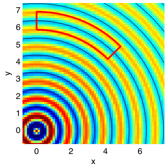
To easily observe the absence or presence of the phase shifts, we plot the resulting wave field on a 45 degree segment of an annulus, with the radial coordinate varying on an interval of about a wavelength. The location where the real part is minimal, according to the exact solution, is indicated by a line that is plotted. The transformation of the field to polar coordinates is done by using cubic interpolation from the numerical solution on a Cartesian mesh. Schematically this is displayed in Figure 4, where part (b) of the figure is a plot in polar coordinates of the indicated region of part (a).
(a)
(b)
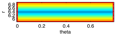
The results from the computations are displayed in Figure 5. Part (a) shows that for second order finite differences at 10 points per wavelength (ppw) a clearly visible phase shift already occurs after 20 wavelengths. In (b) we see that for the JSS method a clearly visible phase shift occurs after 50 wavelengths. In (c), (d) and (e) we investigate the sixth order method CHO6 of [29] at 6, 5 and 4 ppw. (We have chosen one of the higher order methods). At 6, 5 and ppw the maximum phase errors at 500 wavelengths are 0.27, 0.84 and radians respectively and the associated phase shifts are increasingly visible in the pictures. In parts (e) to (i) we plot results for the IOFD method at 6, 5, 4, 3 and 2.5 ppw. At 6, 5 and 4 ppw the maximum phase shifts are 0.0065, 0.020 and 0.089 radians respectively, i.e. considerably smaller than observed for CHO6. At 3 ppw the phase shift after 500 wavelengths is clearly visible, only at 2.5 points per wavelength does it become large and in this case the field is plotted at 100 instead of less than 500 wavelengths from the source.
In Figure 6 we plot the amplitude errors for IOFD at 3 and 4 ppw. For more than 4 ppw they were increasingly small.
(a)

(b)

(c)

(d)

(e)

(f)

(g)

(h)

(i)

(j)

(a)

(b)

In our second example is variable. To avoid that errors due to the discretization of the velocity model become dominant we use use a smoothly varying velocity model, namely a smoothed Marmousi model. In this example we will compare a solution with IOFD using a minimum of six points per wavelength with a fourth order finite element solution using twice as many grid points in each direction. In these examples the right hand side was a point source and the linear systems were again solved with MUMPS. In case of variable coefficients we assumed that is defined on the cell centers. The values of (see (54)) at other points were obtained using linear interpolation from the values of at the cell centers.
The velocity model is given in Figure 7. It is obtained from the Marmousi model by convolving along both of the axes with a cos square pulse of width 160 meter. We will give results for 50 and 100 Hz. A solution for the first case is given in Figure 8. Figure 9 contains four plots. The top plots are reference amplitudes for obtaining relative errors and the bottom two plots are relative errors with respect to the reference values. In both cases we give results for 50 and for 100 Hz. The reference value is a local average of the absolute value of the solution over a square of about 2 by 2 wavelengths. This is done because the solutions themselves contain nodal points from interfering waves, where the amplitude is very small, and are hence not directly suitable as reference value. Very small relative errors are obtained (except directly at the source point), ranging from less than 0.01 over most of the domain to 0.05 or 0.08 at isolated spots where the absolute amplitude is small.


(a) (b)


(c) (d)


7. Application in multigrid based solvers
The last few years there have been several interesting developments in multigrid methods for Helmholtz equations. Different two-grid methods with inexact coarse level solvers have been studied in [5] and [25]. In [5] a number of iterations of shifted Laplacian preconditioned Krylov solver [11] is used as coarse level solver. The method of [25] is based on the multigrid method in [26] with a double sweep domain decomposition preconditioner [24] as coarse level solver. The multigrid method with exact coarse level solver was studied in [26]. There it was shown that the convergence can be strongly improved when phase slowness differences between the fine and coarse scale operators are minimized. For this purpose, optimized finite differences were used at the coarse level, and good convergence was obtained for meshes with downto three points per wavelength at the coarse level. For standard choices of the coarse level discretization it was found that about 10 points per wavelength at the coarse level were needed to have good convergence.
In [26] standard second order finite differences were used as the fine level. Because of the relatively large phase slowness errors of this method, the coarse level optimized finite difference method had to be constructed specifically to match the phase slownesss of second order finite differences, instead of matching the true phase slowness. A better choice is to use method with small phase slowness errors at the fine level and at the coarse levels. Here we will use IOFD at all levels. These experiments do not involve the operator . The operator is used directly as coarse level discretization and at the fine level we are only interested in solving equation (111).
In the first set of computational results of this section we will show that this results in good convergence of the multigrid method with exact coarse level solver. In a second example we will study the multigrid method with inexact coarse level solver of [25].
In our study of the convergence when using the exact coarse level solver we are again interested in examples with wave propagation over hundreds of wavelengths. Therefore, these experiments are done in two dimensions. For background on multigrid methods, see [28]. As in [26] most of the components of the multigrid method are standard. Full weighting restriction and prolongation operators are used. As smoother, an -Jacobi method is used. We found that and (the number of pre- and postsmoothing parameters) are good choices of parameters. In these experiments we used a conventional absorbing boundary layer to simulate an unbounded domain.
We studied the convergence as a function of the number of points per wavelength for three velocity models: A constant model, the Marmousi model and a slice of the 3-D SEG-EAGE salt model. The latter two models are displayed in Figure 10. The parameters of the examples and the observed number of iterations to reduce the residual by are given in 5. At downto three points per wavelength the method behaved well. At 2.5 ppw coarse level the method still converged, but the number of iterations increased substantially, and also became more sensitive to the problem size (which was apparent from smaller scale experiments not included in the table).
Note that the application in multigrid methods is quite different from the application as fine level discretization. The method is used at coarser meshes (at three points per wavelength the direct application will in general lead to too large errors). Also, multigrid solvers using IOFD at coarse levels may be developed for other types of fine level discretizations, as long as they use a regular mesh.
(a)

(b)

| constant | Marmousi | salt model | ||||
| ppw | freq | its | freq | its | freq | its |
| 5 | 480 | 29 | 150 | 23 | 60 | 18 |
| 6 | 400 | 8 | 125 | 11 | 50 | 8 |
| 7 | 342.9 | 6 | 107.1 | 9 | 42.9 | 7 |
| 8 | 300 | 5 | 93.8 | 8 | 37.5 | 6 |
| 9 | 266.7 | 5 | 83.3 | 7 | 33.3 | 6 |
| 10 | 240 | 4 | 75 | 6 | 30 | 5 |
We now turn to a multigrid method with an inexact coarse level solver. Such methods are used because in three dimensions it is often too expensive to compute the exact solution. These methods are currently some of the fastest solvers for large problems that are in the literature [5, 25].
Because we are interested in coarse meshes, such as six points per wavelength based on the previous examples, it is a priori not clear that the above mentioned solvers perform well. Like many solvers in the literature, they were tested for problems with at least ten mesh points per wavelength. They cannot be assumed to converge as well for larger frequencies, because multigrid convergence depends on frequency, and the same is true for the shifted Laplacian preconditioner [9]. For the double sweep domain decomposition it is unclear how the frequency affects the convergence, but a priori it also cannot be assumed to be independent of the frequency.
This raises the question whether we can actually obtain a gain in efficiency by going to coarser meshes. The purpose of the next example is to show that this indeed the case, and to generally show that IOFD can perform well with the solver of [25].
In the following example we will test the method of [25], which is a two-grid method using an inexact coarse level solver given by a double sweep domain decomposition preconditioner (see [24]). The method is modified to use IOFD at both the fine and the coarse levels of the two-grid method. We will take the SEG-EAGE Salt Model as an example, similarly as in [25]. In addition to changing the discretization method we will increase the frequency by a factor , so that a minimum of six points per wavelength is used, a regime which has not been tested before for this method. If convergence and cost per degree of freedom would stay constant, there would be an improvement in the cost by a factor of over (more than this because cost grows somewhat faster than linear with problem size).
The original SEG-EAGE salt model is of size 13500 x 13500 x 4200 meter, discretized with 20 m grid spacing. We apply the method just described to solve the Helmholtz equation with this velocity model and random or point sources as right hand sides at four different frequencies from to Hz. Slices of the model are displayed in Figure 11. Parameters in the two-grid method are for the number of pre- and postsmoothing steps and in the -Jacobi method. Computations were done on the Lisa cluster at Surfsara, described already in section 6, using the implementation described in [25]. A maximum of 16 nodes were used in parallel for these computations.
The algorithm is set up to solve for multiple right hand sides simultaneously. In the table of results, the computation time per right hand side is given. In Table 6 some parameters are given, together with the computation time and iteration count to reduce the residual by . As illustration, plots of a solution are given in Figure 12. It can be observed that the cost increases very little compared to the results of [25], even though frequencies are increased by a factor . Some increase in cost can be expected, because the discrete Helmholtz operator using second order finite differences is cheaper to apply than the one using a compact 27-point stencil. Hence reducing the number of points per wavelength in the mesh can indeed lead to corresponding savings in computation time.
As mentioned, the methods of [5] and [25] are some of the fastest currently in the literature. Comparing with these results we see a significant improvement. For example in [5] the SEG-EAGE salt model problem was solved at 10 Hz in 270 seconds on 256 cores of an IBM BG/P machine (with the residual reduced by a factor instead of in our case). Here we solve the problem at 9.91 Hz using 128 cores in 45 seconds per right hand sides (179 seconds for four right hand sides), a clear improvement33 3 On the other hand the method of [5] uses less memory and has been applied to larger examples than we have shown here. Furthermore no full comparison including accuracy was made..
(a) (b)


(a) (b)


| frequency | 6.25 | 7.87 | 9.91 | 12.5 |
|---|---|---|---|---|
| size | 338x338x106 | 426x426x132 | 536x536x166 | 676x676x210 |
| # dof | ||||
| cores | 32 | 64 | 128 | 256 |
| # of rhs. | 1 | 2 | 4 | 8 |
| iterations | 12 | 12 | 13 | 15 |
| computation time/rhs(s) | 26 | 35 | 45 | 73 |
8. Discussion
Here we summarize some of the conclusions and further discuss the results.
Using the results presented one can make a case for the use of coarse meshes using a minimum of five or six points per wavelength in time harmonic wave simulations in case is smooth. This idea is not new, in the exploration geophysics community it appears to be quite common. However, we found that the methods that have been proposed for this purpose in [16] and [21] can be expected to give substantial phase errors in simulations of large distance wave propagation. By using the new IOFD method (in two or three dimensions) or the QS-FEM method (in two dimensions only), phase errors can be made much smaller.
In has strong gradients, one can expect that, at least locally where is large, finer meshes and/or different discretizations are needed to obtain accurate solutions. Large gradients lead to reflections. Typically finer meshes are needed to model these accurately. For one reason this is because finer discretizations of are needed, since linearized scattering theory shows that reflected waves are associated with perturbations in the medium velocity with wave vectors of length up to (where here refers to the background velocity around which the linearization is applied). However, in this case the multigrid approach discussed in section 7 can still be useful. It has been applied in successfully in examples with discontinuities. This suggests to do further research on multigrid approaches with compact finite difference method at the coarse level and other discretizations at the fine level, including methods with local refinement. A similar argument can be held for the discretization of the right hand side in the equation . For rapidly varying functions , finer meshes may be needed at least locally where the rapid variations occur.
When applied in inversion algorithms IOFD and QS-FEM are somewhat more complicated than the methods of [16] and [21], because the operatore depends in a more complicated fashion on the coefficients, which means it is more complicated to compute the derivative of the finite difference operator with respect to the medium coefficients. Due to the use of Hermitian interpolation, these derivatives are however continuous for our IOFD method.
References
- [1] S. Alinhac and P. Gérard. Pseudo-differential operators and the Nash-Moser theorem, volume 82 of Graduate Studies in Mathematics. American Mathematical Society, Providence, RI, 2007. Translated from the 1991 French original by Stephen S. Wilson.
- [2] P. R. Amestoy, I. S. Duff, J. Koster, and J.-Y. L’Excellent. A fully asynchronous multifrontal solver using distributed dynamic scheduling. SIAM Journal on Matrix Analysis and Applications, 23(1):15–41, 2001.
- [3] I. Babuška, F. Ihlenburg, E. T. Paik, and S. A. Sauter. A generalized finite element method for solving the Helmholtz equation in two dimensions with minimal pollution. Comput. Methods Appl. Mech. Engrg., 128(3-4):325–359, 1995.
- [4] J.-P. Berenger. A perfectly matched layer for the absorption of electromagnetic waves. Journal of Computational Physics, 114(2):185–200, 1994.
- [5] H. Calandra, S. Gratton, X. Pinel, and X. Vasseur. An improved two-grid preconditioner for the solution of three-dimensional Helmholtz problems in heterogeneous media. Numer. Linear Algebra Appl., 20(4):663–688, 2013.
- [6] Z. Chen, D. Cheng, and T. Wu. A dispersion minimizing finite difference scheme and preconditioned solver for the 3D Helmholtz equation. Journal of Computational Physics, 231(24):8152 – 8175, 2012.
- [7] W. C. Chew and W. H. Weedon. A 3D perfectly matched medium from modified Maxwell’s equations with stretched coordinates. Microwave and optical technology letters, 7(13):599–604, 1994.
- [8] G. C. Cohen. Higher-order numerical methods for transient wave equations. Scientific Computation. Springer-Verlag, Berlin, 2002. With a foreword by R. Glowinski.
- [9] S. Cools and W. Vanroose. Local Fourier analysis of the complex shifted Laplacian preconditioner for Helmholtz problems. Numer. Linear Algebra Appl., 20(4):575–597, 2013.
- [10] J. J. Duistermaat. Fourier integral operators, volume 130 of Progress in Mathematics. Birkhäuser Boston, Inc., Boston, MA, 1996.
- [11] Y. A. Erlangga, C. W. Oosterlee, and C. Vuik. A novel multigrid based preconditioner for heterogeneous Helmholtz problems. SIAM J. Sci. Comput., 27(4):1471–1492 (electronic), 2006.
- [12] G. Grubb. Distributions and operators, volume 252 of Graduate Texts in Mathematics. Springer, New York, 2009.
- [13] I. Harari and E. Turkel. Accurate finite difference methods for time-harmonic wave propagation. J. Comput. Phys., 119(2):252–270, 1995.
- [14] L. Hörmander. The analysis of linear partial differential operators. III, volume 274 of Grundlehren der Mathematischen Wissenschaften [Fundamental Principles of Mathematical Sciences]. Springer-Verlag, Berlin, 1985. Pseudodifferential operators.
- [15] F. Ihlenburg. Finite element analysis of acoustic scattering, volume 132 of Applied Mathematical Sciences. Springer-Verlag, New York, 1998.
- [16] Jo, Churl-Hyun and Shin, Changsoo and Suh, Jung Hee. An optimal 9-point, finite-difference, frequency-space, 2-D scalar wave extrapolator. Geophysics, 61(2):529–537, 1996.
- [17] S. G. Johnson. Notes on perfectly matched layers. http://math.mit.edu/ stevenj/18.369/pml.pdf, 2010.
- [18] H. Knibbe, W. A. Mulder, C. W. Oosterlee, and C. Vuik. Closing the performance gap between an iterative frequency-domain solver and an explicit time-domain scheme for 3D migration on parallel architectures. GEOPHYSICS, 79(2):S47–S61, MAR-APR 2014.
- [19] M. J. Lighthill. Studies on magneto-hydrodynamic waves and other anisotropic wave motions. Philos. Trans. Roy. Soc. London Ser. A, 252:397–430, 1960.
- [20] J. M. Melenk and S. Sauter. Wavenumber explicit convergence analysis for galerkin discretizations of the helmholtz equation. SIAM J. Numer. Anal., 49(3):1210–1243, June 2011.
- [21] S. Operto, J. Virieux, P. Amestoy, J.-Y. L’Excellent, L. Giraud, and H. B. H. Ali. 3D finite-difference frequency-domain modeling of visco-acoustic wave propagation using a massively parallel direct solver: A feasibility study. Geophysics, 72(5, S):SM195–SM211, 2007.
- [22] J. Poulson, B. Engquist, S. Li, and L. Ying. A parallel sweeping preconditioner for heterogeneous 3D Helmholtz equations. SIAM J. Sci. Comput., 35(3):C194–C212, 2013.
- [23] C. D. Riyanti, A. Kononov, Y. A. Erlangga, C. Vuik, C. W. Oosterlee, R.-E. Plessix, and W. A. Mulder. A parallel multigrid-based preconditioner for the 3d heterogeneous high-frequency helmholtz equation. Journal of Computational Physics, 224(1):431 – 448, 2007. Special Issue Dedicated to Professor Piet Wesseling on the occasion of his retirement from Delft University of Technology.
- [24] C. C. Stolk. A rapidly converging domain decomposition method for the Helmholtz equation. J. Comput. Phys., 241:240–252, 2013.
- [25] C. C. Stolk. A two-grid accelerated sweeping preconditioner for the Helmholtz equation, 2014. Arxiv.org/abs/1412.0464.
- [26] C. C. Stolk, M. Ahmed, and S. K. Bhowmik. A multigrid method for the helmholtz equation with optimized coarse grid corrections. SIAM Journal on Scientific Computing, 36(6):A2819–A2841, 2014.
- [27] G. Sutmann. Compact finite difference schemes of sixth order for the Helmholtz equation. J. Comput. Appl. Math., 203(1):15–31, 2007.
- [28] U. Trottenberg, C. W. Oosterlee, and A. Schüller. Multigrid. Academic Press Inc., San Diego, CA, 2001. With contributions by A. Brandt, P. Oswald and K. Stüben.
- [29] E. Turkel, D. Gordon, R. Gordon, and S. Tsynkov. Compact 2D and 3D sixth order schemes for the Helmholtz equation with variable wave number. Journal of Computational Physics, 232(1):272 – 287, 2013.
Appendix A Phase slowness computations for finite element methods
In a periodically repeating setting, which is the case for finite elements with , the situation is somewhat more complicated. The symmetry property (109) only holds for divisible by . For such operators we consider the Bloch waves
| (121) |
where is periodic with shifts , integers. For given , the action of an operator with these symmetries is given by an matrix acting on the (in three dimensions) for . We need to find the vectors for which there is a zero eigenvalue. However not all zero eigenvectors correspond to plane waves with wave vectors , because of the presence of . In general can correspond to a linear combination of plane waves with wave vectors given by , where are integers. Assuming that some corresponds to a simple zero eigenvalue and that is close to a plane wave (which is often the case because the eigenfunctions of the continuous operator are plane waves and the operator is a good approximation of the continuous operator), these integers can be determined modulo , and the wave vector associated with an element of the zero set of can be determined.
In the computations we will take a somewhat different approach. We will compute all eigenvalues, and then only consider the one whose eigenvector is most closely correlated with (has the in absolute value largest inner product with) the constant function . We will say we have found a phase velocity vector at some if this eigenvalue is zero. This approach has some limitations, but a more extensive study of this topic falls outside the scope of this paper. For standard finite elements and such that the mesh has more than four points per wavelength this appeared to be sufficient.