A Complete Worst-Case Analysis of Heapsort with Experimental Verification of Its Results
A manuscript (MS) intended for future journal publication
Note: ©2015 Marek A. Suchenek.
Abstract
Main results. A rigorous proof that the number of comparisons of keys performed in the worst case by on any array of size is equal to:
where , given by:
is a function of with the minimum value 0 and and the supremum value
is the sum of all digits of the binary representation of , is the exponent of in the prime factorization of , and is a binary function on the set of integers defined by:
is presented.
An algorithm that generates worst-case input arrays of any size for is offered. The algorithm has been implemented in Java, runs in time, and allows for precise experimental verification of the above formula.
Significance. The worst-case behavior of has escaped mathematically precise characterization for almost five decades now. This paper fills that important gap. The exactness of the derived number of comparisons of keys performed by in the worst case, as opposed to merely big-oh or asymptotic approximation or bound, allows for direct and definite experimental verification of its correctness.
Keywords:
Heap , heapsort , sorting , sum of digits , worst case.2010 MSC
68W40 Analysis of algorithms ,2010 MSC
11A63 Radix representationACM Computing Classification
Theory of computation: Design and analysis of algorithms: Data structures design and analysis: Sorting and searching
Mathematics of computing: Discrete mathematics: Graph theory: Trees
Mathematics of computing: Continuous mathematics: Calculus
Introduction
Many of those who could not figure it out exactly were quick to dismiss the importance of precisely knowing it. But there are some significant advantages of knowing the exact value as opposed to its approximation. For one, it can be conclusively verified by means of a direct experiment.
Some researchers tend to believe that undergraduate Computer Science is not an area for intellectually challenging and interesting problems. Some even go as far as to dismiss pursuit of their solutions as pedagogy. But such a prejudice appears, well, prejudice, as there do exist questions that belong to undergraduate CS, yet they have been declared difficult to answer even by some renowned scholars. Although the deceitful simplicity of some of the solutions of problems that were once considered hard might prompt a skeptic to entrench himself in his dismissiveness, it should not puzzle those sympathetic to the conjecture, one of the consequences of which stipulates the existence of hard to solve problems whose solutions are straightforward to verify as soon as their witnesses have been found.
Take, for instance, invented by Williams [11] and enhanced by Floyd [4]. This specimen of elegance and simplicity, and a classic that has been taught across curricula of virtually every ABET-accredited Computer Science program, does belong to to undergraduate CS, yet it apparently has resisted attempts of some seasoned researchers to accurately characterize its worst-case performance. In this article, I will use rather elementary mathematics to bring the worst-case analysis of to the point that one could consider complete.
The analysis I present here is not particularly short11 1 The rigorous proof of the main result is rather lengthy, particularly when compared to the short and elegant algebraic derivation in [10] of a similar result for the Floyd’s heap-construction program that constitutes the first (and faster) half of the .. This does not come as a total surprise, taking into account almost five decades that passed without its completion. Although Shaffer and Sedgewick declared long time ago that their paper [9] “essentially complete[d] the analysis of [],” they also admitted that “there [was] another quantity that contribute[d] to the leading term of the running time that require[d] more intricate arguments,” for which they had “little specific information about the distribution beyond what [was] implied by [their] asymptotic results.” Clearly, they did not attempt to derive the exact formula for the number of comparisons of keys that performs, which remained unknown for 49 years.
So, here it is: for every natural number , the number of comparisons of keys performed in the worst case by the on any array of size is equal to:
where , given by:
is a continuous function (visualized on Figure 32 page 32) of on the set of reals , with the minimum value 0 and and the maximum (supremum, if is restricted to integers) value
is the sum of all digits of the binary representation of , is the exponent of in the prime factorization of , and is a binary function22 2 Algebraically, . (visualized on Figure 23 page 23) on the set of integers defined by:
Moreover, if then the above formula simplifies to:
The method I chose for my derivation the above formula could be characterized mostly as a brute force approach, with some subtler inductive arguments without which the brute force alone would not accomplish much. Nevertheless, the elementary algebra involved in it seems well-worth studying in its own right as it also applies to other problems that are related to sorting and to finite binary trees.
1 An overview
The main subject of my analysis is the number of comparisons of keys that Williams’ vanilla with Floyd’s improvement performs in the worst case while sorting an -element array of distinct integers. It consists of three major parts. The goal of the first part is to show that the said worst case number of comparisons is the sum of the respective numbers and for the heap-construction phase and the heap-deconstruction phase . The goals of the second and the third part are to derive the formulas for and . Those three, once completed, yield the formula for .
The first part turned up the easiest of the three. Running backwards on any given heap resulted, and provably so, in an array that would turn onto while performing the maximal possible number of comparisons for any array of that size.
The second part was somewhat harder; however, it has been recently nailed down with a simple closed-form formula for that had a succinct and elegant algebraic proof33 3 See [10] for such a proof..
The third part was considerably more complicated than the other two. A fairly simple strategy for generating bad cases for by running it backwards led to a straightforward44 4 At least for those fluent with the kind of math that I am using in this paper., if a bit tedious, derivation of a closed-form formula for a lower bound of , but that lower bound was less than the ‘‘easy’’ upper bound55 5 . of I knew. It was the demonstration that the said strategy could not be beaten, which fact allowed me to conclude that the derived lower bound was also an upper bound and yielded a proof of the closed-form formula for , that was surprisingly66 6 It did look at the beginning as a simple exercise, only to turn out elusive as it kept evading my attempts to be formulated precisely. convoluted and resistant to simplifications.
Well, there must have been a reason why, to my best knowledge, a journal-quality proof of the worst-case formula had not been published despite the fact that it had been done, even if in a somewhat rough form, for the special case of inputs of the size some 36 years ago. After finishing the said proof I think I got a pretty good idea why all those who attempted it might have given up before bringing their efforts to a conclusive end.
Out of several factors that made such a proof not quite a routine exercise, a flaw in the structure of the worst-case heaps for deserves a special mention. It turns out that the number of hereditary77 7 A heap is a hereditary worst-case heap if, and only if, it is a worst-case heap and is either empty or is a hereditary worst-case heap. worst-case heaps for is finite88 8 The fact that not all worst-case heaps are hereditary worst-case heaps follows also from the fact that the number of comparisons of keys that the operation performs on a worst-case heap on nodes is not a function of . (1017 to be exact), which rules out the existence of any greedy scheme of generating worst-case heaps for of arbitrary size (greater than 22). As a result, the proof of the said formula hangs on a singularity of worst-case heaps which states that if and is a heap on nodes such that the execution of on performs the maximum , over all heaps on nodes, number of comparisons of keys then the heap produced by the execution of is not a worst-case heap99 9 It is a singular property, indeed, as for every , there is a worst-case heap on nodes with such that is a worst-case heap.. Laying down foundations for a demonstration of the above fact was perhaps the most tedious task in this study.
Here is a road map of the paper.
Section 2, page 2 and on, lays down basic definitions and algebraic facts related to the subject matter.
Section 3, page 3 and on, introduces notation that I use in this paper, some of which may differ from the notation used by other authors.
Section 4, page 4 and on, describes a basic technique for constructing worst cases for and its components by running them backwards. Methods , , and are introduced there.
Section 5, page 5 and on, presents a constructive proof that the exact characterization of the worst-case performance of may be computed as a sum of exact characterizations of the worst-case performances of its two phases: the heap-construction phase (for which a closed-form formula has been recently discovered) and the heap-deconstruction phase. This is accomplished by demonstrating that for any heap of nodes, method - a reverse of - constructs an -element array that constitutes a worst-case array for the heap-construction phase.
At this point, the only piece of information that is needed for the exact characterization of the worst-case performance of the entire is a formula for the worst-case performance of the heap-deconstruction phase.
Section 6, page 6 and on, introduces a solitaire game of Pull Downs a payoff of which is equal to the number of comparisons of keys that are needed to deconstruct a heap produced by the game. The said payoff is maximal if, and only if, the produced heap is a worst-case heap. The Section establishes some correspondences between heaps produced by the game and various generators of the game, which provides some notational convenience needed in the remainder of the paper and assures consistency of the derived results. The above facts reduce the problem of construction of a worst-case heap for the heap-deconstruction phase of to the problem of finding a generator of a suitable game that yields a maximal payoff.
Section 7, page 7 and on, contains definitions and technical details of computations of credits for moves in the game of Pull Downs. It provides characterization of moves that yield maximal credits and evaluates losses of credits for some sequences of moves.
Section 8, page 8 and on, is mostly notational. It introduces the concept of a strategy and defines various forms of payoffs, including the upper-bound payoff, and losses of credit related to it.
Section 9, page 9 and on, introduces some special strategies for the game of Pull Downs: a sub-optimal strategy and a family of strategies (one strategy for each ), each being optimal for given . Strategy is sub-optimal in that it loses 1 credit per level, relative to the upper-bound payoff, of the heap constructed, from the level 3 on, and is optimal for each complete1010 10 On nodes, that is. heap it constructs. It also maintains certain invariant property of the heaps it produces that is needed for the demonstration of optimality of its improvements. For each , the strategy improves upon (by the total of 1 credit) in that, unlike , it is greedy in the level of the heap constructed, so that it postpones the 1 credit loss in that level until no further postponement is possible1111 11 Until the move .. The payoffs for those strategies are derived there. They establish a lower bound for the worst-case behavior of the heap-deconstruction phase.
Section 10, page 10 and on, is devoted to proofs of optimalities of strategies and . The optimality of allows me to conclude that the lower bound derived in Section 9 and given by the formula for payoffs for is an upper bound, too, thus yielding the sought-after characterization of the worst-case behavior of the heap-deconstruction phase. The mostly case-driven proof uses, at some point, the fact that no strategy can gain relative to a strategy that is optimal for complete heaps (in particular, relative to and ) more than 1 credit an any level of the heaps that it produces. It allows strategies that are optimal for complete heaps and greedy in the levels of heaps they construct to collect the maximal payoffs and, therefore, be optimal. It also reduces considerably the number of cases that need to be tackled in the said proof.
Subsection 10.1, page 10.1 and on, attempts to explain why the optimality proof I present in this paper is more complicated than one could expect it to be.1212 12 The singularity of worst-case heaps of size , indicated on page 8, seems to be the culprit here. It derives some intuitively simple facts1313 13 The most basic of which is the Singularity Theorem 10.13, page 10.13, stating that no worst-case heap of size admits a lossless pull down. that entail the optimality of , and demonstrates that they are about as difficult to prove as those in Section 10.
The remainder of the paper easily follows from the above.
Section 11, page 11 and on, proves a closed-form formula for the worst-case number of comparisons of keys performed by the heap-deconstruction phase of .
Section 12, page 12 and on, proves two closed-form formulas for the worst-case number of comparisons of keys performed by the , one with function floor and one (mostly) without it.
Section 13, page 13 and on, analyses the behavior of the “jumpy” term in the mentioned above formulas and offers its tight upper bound expressed by a function that is continuous on the set of reals except for .
Section 14, page 14 and on, comments on the origins of this article, with Subection 14.1, page 14.1 and on, comparing the presented results to those published in an old report by Kruskal and Weixelbaum.
A offers illustrating examples. A.1, page A.1 and on, shows details of construction of a -element worst-case heap for the heap-deconstruction phase of in first 11 moves of strategy . A.2, page A.2 and on, shows details of construction of the last level of a -element worst-case heap for the heap-deconstruction phase of in moves 15 through 30 of strategy . A.3, page A.3 and on, shows program-generated examples of 500-element worst-case array for the heap-construction phase and 500-element worst-case heap for the heap-deconstruction phase of .
2 Heaps and Heapsort - a brief review
I am going to use extensively some standard undergraduate math of analysis of algorithms in this paper. Here is a quick reminder of some basics: is a logarithm base 2 of ; is the greatest integer not greater than ; is the least integer not less than ; thus is the greatest power of 2 not larger than and is the least power of 2 not less than ; and is the remainder modulo function defined for by .
Here is an ubiquitous formula that comes handy while dealing with this kind of math, true for every positive integer :
| (1) |
a special case of which yields, for every positive integer :
| (2) |
The rest of this Section contains some standard definitions and basic facts pertaining to heaps and that those familiar with the subject may wish to omit and go directly to the next section on page 3. Unlike many other presentations, this one is prevailingly algebraic.
A binary tree structure is a non-empty1414 14 Allowing empty trees and heaps does not add any benefits to the presentation of this paper. finite set of positive integers, referred to as the index set, that is closed under positive integer division by 1515 15 This coincides with the usual mathematical-logical definition of binary tree (cf. [7]) as a set of binary sequences of length (where is an ordinal number) for closed under truncation, taking into account that every finite binary sequence is equal to the binary representation of some integer with the leading 1 omitted; however, mine does not include the empty tree., under convention that positively-integerly divided by is equal to . A finite binary tree, to which I will simply refer to as binary tree, is a function whose domain is . The elements of (ordered pairs , that is) are called nodes. For the sake of simplicity of presentation, I will assert that the said function is , which in more humane terms means that the tree in question is duplicate-free. In particular, has the inverse function . Thus 1616 16 I use the square brackets in lieu of parentheses here because of popularity of an array representation of binary trees. is the value stored in at index and is the index of the value in tree . This -ness assertion will allow me to sometimes not distinguish between the nodes and their constituent indicies and values if it is clear from the context which of the three notions am I referring to. Since the sole purpose of this article is analysis of the worst-case number of comparisons of keys performed by the sorting algorithm and its components, the above assertion does not lead to a loss of generality. Moreover, since the operation is not used in , so is neither included nor discussed in this analysis, I may1717 17 And, usually, will. assume, without loss of generality, that is a permutation on 1818 18 Thus the inverse of is a permutation, too; for example, the inverse of is ., that is, that the range of coincides with .
The index set of a binary tree defines the parent-children relationship between its nodes. A node at index is a parent of a node at index , or - in other words - a node at index is a child of a node at index if, and only if,
| (3) |
An iterative application of (3), taking into account that , gives rise to the definition of the usual ancestry relation between nodes at indicies (an ancestor’s index) and (a descendant index) in terms of existence of for which the equality
| (4) |
is satisfied. The equation (4) yields the inequality
| (5) |
which implies
| (6) |
or
| (7) |
Thus, for any , is the index of an ancestor of a node at index if, and only if,
| (8) |
Plugging (7) into (5) yields another, equivalent to (8), characterization of the ancestry relation:
| (9) |
The equality (3) has two solutions:
| (10) |
The node is called the left child of at index if, and only if, its index is , and is called the right child of if, and only if, its index is .
The root is defined as the node with no parent; thus is the index of the root2020 20 Because and .. A leaf is defined as a node without children; thus its index satisfies the condition
| (11) |
where is the index set of the tree.
A path2121 21 From the root. in a binary tree is a sequence of indicies of defined by induction: is a path in , if is a path whose last element is and is an index in with then the concatenation is a path in , and nothing else is a path in .
It follows that binary representations of the indices of a binary tree provide the navigation information how to get to those nodes from the root, with 0 meaning “go to the left child” and 1 meaning “go to the right child”, except for the first 1 that means “go to the root”, as it has been visualized on Figure 1 page 1. In that sense, each of those indices encodes the path (from the root) to the node at that index. Naturally, the length of such path is one less than the number of digits in the binary representation of , that is, it is equal to
| (12) |
where is the index of the destination node (the last index in the said path). I will call the depth of the node at index . Moreover, I will call a level of the tree the set of all its nodes (or, sometimes, indicies thereof) that have depth . Thus every node belongs to the level , where is the index of that node.
In particular, the (binary representation of the) largest index in a binary tree encodes the path (from the root of the tree) to its last node. Because that path is a longest path in the tree, its length
| (13) |
also the depth of the node at index , is the depth of the entire tree. Thus the depth of the tree is the level number of the last non-empty level of that tree.
Given a binary tree , the path of the largest child is defined as the path (from the root) to a leaf such that each node in , except for the root, is the largest child of its parent. One can easily conclude from the -ness assertion that every binary tree has the unique path of the largest child. If may not go all the way down to a leaf then I will call it a path of the largest child.
Each node at index in a binary tree is the root of a subtree that consists of and all its descendants, and - when treated as a separate entity - has it own index set . It can be computed with a help of the formula (7) page 7 for the length of path from to as
| (14) |
where is the index set of and the ancestry relation between the respective indicies and is given by (8) page 8. 2222 22 If then is not necessarily a permutation on its index set .
The height of a node at index in a binary tree is defined as the depth of the subtree of .
I call a binary tree a convex binary tree if, and only if, its index set is a convex set of integers. Thus every convex binary tree on nodes has the index set equal to
| (15) |
One can conclude from (14) that any subtree of a convex tree is convex.
It follows from (12) and (14) that the depth of a subtree of a convex tree of nodes is equal to
[since (8) and (9) page 9 are equivalent]
| (16) |
Since the maximal that satisfies (9) must also satisfy
| (17) |
(or otherwise it would not be maximal that satisfies (9)), I conclude from (17) that
or
| (18) |
Applying (18) to (16), I obtain one of the fundamental formulas for the precise worst-case analysis of the heap construction phase of
| (19) |
If the convex binary tree in question has more than 1 node then the number of nodes in its last level is odd if, and only if, the number of nodes in the entire heap is even.
It follows from (11) and (15) that is an index of a leaf in a convex binary tree if, and only if,
| (20) |
where is the size of the index set.
The leftmost descendant of a node at index in a finite convex binary tree is the first (leftmost) node in the last nonempty level of subtree . By virtue of (9) page 9, (18), and (19), its index is given by this formula:
| (21) |
Every non-empty level in any convex binary tree, except, perhaps, the last non-empty level, is equal to , while the last non-empty level in such a tree is equal to .
Moreover, I call a complete binary tree a convex binary tree whose index set has the size , that is,
| (22) |
Naturally, any subtree of a complete binary tree is a complete binary tree. Of course, is the size of the index set of a complete heap if, and only if, is a power of two, that is, , or, by (1) page 1,
| (23) |
Also, the largest complete binary tree of no more than nodes has
| (24) |
nodes, since is the greatest power of 2 not greater than so that is the greatest power of 2 minus 1 not greater than . By (2) page 2 and (13) page 13, the depth of such largest complete binary tree of no more than nodes is
| (25) |
A heap is a convex2727 27 Some authors use adjective complete in this context, instead. A neat definition borrowed from mathematical logic allows one to identify the set of indicies of a countable -ary tree with a set of positive integers closed under positive integer division by , with assumed equal to if . In light of such a definition, a finite convex -ary tree has a set of indicies that comprises of the first positive integers, which one could describe as complete, although is in fact a convex set of integers so the adjective convex appears like a better descriptor of tree . I will reserve adjective to binary trees with nodes, where is a positive integer. It is worth noting that in mathematical logic trees were studied long before they were used in Computer Science, using a definition of a complete -ary tree that ours is compatible with; in particular, according to that definition (cf. [7], p. 381), a finite complete -ary tree of depth D has nodes., partially ordered binary tree. Partially ordered means that every sequence of values along any path in the tree is ordered in a decreasing order.
An example of a heap is visualized on Figure 1.

Quite obviously, any non-empty convex binary tree may be represented as a one-dimensional array whose indicies range over the index set of , that is, from to , the number of nodes of the tree.
| index | 1 | 2 | 3 | 4 | 5 | 6 | 7 | 8 | 9 | 10 | 11 | 12 |
|---|---|---|---|---|---|---|---|---|---|---|---|---|
| value | 12 | 11 | 7 | 9 | 10 | 2 | 3 | 6 | 8 | 4 | 5 | 1 |
The table in Figure 2 shows an array that represents the heap of Figure 1 with the indices of the array shown in the top row of the table.
If tree is partially ordered then its every subtree , where is in the index set of , is partially ordered as well, so a subtree of a heap is a heap2828 28 Except that it is not necessarily a permutation on its index set.. I will call a subheap of .
Heapsort (see, e.g., [5] for its description and partial analysis) consists of two phases: heap construction and a sequence of removals from the constructed heap that I call heap deconstruction.
Both phases use a subroutine FixHeap that inherits an almost heap, defined as a heap whose root, referred to in some contexts as a patch, may violate the partially ordered tree condition in the definition of heap, and turns it onto a heap by bubble-sorting its root into the path of the largest child. This is done by demoting the said patch down the heap while promoting the largest of its current children until the demotee reaches the level where it is not less than any of its current children, if it still has any at that level. Since each step in that process requires comparing, directly or indirectly, the demotee to its all children2929 29 Clearly, the demotee must have been compared to its largest child; knowing which child is the largest does require comparing children to each other, if there are two children, that is., the total number of comparisons of keys that FixHeap performs during one call is equal to the total number of children of elements of the path of demotion that it follows3030 30 Which is a path of the largest child.. Because FixHeap is the only part of Heapsort that performs comparisons of keys, the above characterization is the point of departure of the analysis presented in this paper.
The heap-construction phase, referred to as in this paper and credited to Floyd [4], inherits an array that represents a convex binary tree and rearranges it onto a heap by calling for its parts that represent subtrees of that have been already rearranged onto almost subheaps, beginning from the one that has the last non-leaf (stored at the index in the array) of as the root3131 31 MakeHeap could have begun calling FixHeap from the last node of , but this would produce the same sequence of comparisons of keys and demotions because FixHeap does not do anything to a one-node tree. and ending with the entire tree (the root of which is stored at index ). This is accomplished by the following Java statement:
| for (int i = N/2; i > 0; i--) FixHeap(i); | (26) |
The heap-deconstruction phase, referred to as RemoveAll in this paper, consists of calls to a subroutine RemoveMax. Each of these calls removes the current root of the heap, patches the resulting vacancy with the current last node of the heap, and calls in order to turn the resulting almost heap onto a heap after each removal. The removed nodes are then stored in the array from the last index up in the order they were removed, which process yields an array that is sorted in an increasing order. This is accomplished by the following Java statement:
| for (int i = N; i > 0; i--) heap[i] = RemoveMax(); | (27) |
A complete code of HeapSort may be easily found in about every standard text on Data Structures and Algorithms, or in [12].
3 Notation and basic facts
I am going to measure the running time of Heapsort and its components by the number of comparisons of keys that they perform, using the following notation.
For any operation , denotes the number of comparisons of keys that performs while executed on its input . For instance, , which I will also denote as , is the number of comparisons of keys that the FixHeap performs while turning the almost subheap rooted at node of a convex binary tree onto a heap.
Moreover, denotes the maximum number of comparisons of keys that performs while executed on its any valid input of size . It is given by this formula:
| (28) |
For instance,
| (29) |
Residue3232 32 Proper residue would be a more adequate but longer term. of a heap is either the heap that is the result of one applications of to , or a residue of a residue of .
is the set of all non-negative integers. is the set of all positive integers. A (non-empty) sequence is a function whose domain is a convex subset of that contains 1. If is a sequence and then is the result of restricting (of the domain of ) to N. is the concatenation of sequences and .
4 A useful trick: Running Heapsort backwards
It turns out that is invertible, and so are , , and . This fact allows for running the entire backwards in order to produce inputs that force it to follow predetermined paths of demotions within the heap. This is useful in construction of cases that establish lower bounds on its worst-case behavior. Although the transition relation for , a deterministic algorithm, is a function, its inverse relation is not a function. So, some extra information is required in order to execute it backwards.
The basic operation I will use to accomplish all the above is whose Java code is shown on Figure 3 on page 3. It takes a convex binary tree and two indicies in , and , with a presumed descendant of ,3333 33 It actually works fine even if is not e descendant of ; in such a case, it works as if were equal to 1. removes and returns node (instructions in lines 476 and 481 of the referenced above Java code), and demotes ’s all proper ancestors in that are descendants of (the -loop in lines 478 and 479 of the Java code).
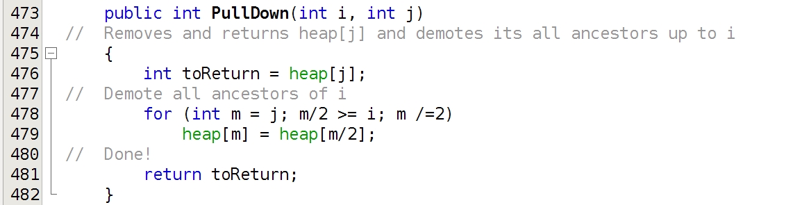
The following Subheap Repair Lemma provides a useful characterization of the implementation of the operation .
Subheap Repair Lemma 4.1
Let be a convex binary tree of nodes, be its index such that the subtree roted at is a heap, be a proper descendant index of in , and be the convex binary tree that is the result of executing the following Java instruction
| H.heap[j] = H.PullDown(i,j); | (30) |
on , where the Java code of method is visualized on Figure 3.
- (i)
The execution of on yields , that is,
(31) - (ii)
The number of comparisons of keys performed by the execution of on is given by this equality:
(32) where
(33) is the number of children of the node at index in a heap of elements.
- (iii)
If is the leftmost descendant of in , and, therefore, in , then the number of comparisons of keys performed by the execution of on is maximal, that is, it satisfies the equality
(34)
Proof Because is a heap and is a proper descendant of in and, therefore, in ,
| (35) |
Moreover, for every child of in and, therefore, in ,
| (36) |
Since, as an effect of instruction (30), , , inequality (35) implies
| (37) |
and inequality (36) implies, for every child of (unaffected by instruction (30)) in in and, therefore, in ,
| (38) |
Each node demoted as a result of in instruction (30) becomes the largest child after the demotion, so that the path of such demotions becomes a path of the largest child in the subtree of . This is a consequence of the fact that each demotee was the parent (before the demotion) of its sibling (after the demotion), except for the case when the demotee became a leaf in , thus it must be greater than its sibling (after the demotion), if it has any. Thus the demotions of done by the subsequent execution of will follow and terminate after is demoted to index since all children of are, by virtue of (38), less than the demotee . As a result, (31) holds. This completes the proof of (i).
The number of comparisons of keys performed by following a path of the largest child is equal to the total number of children of indicies in . Thus,
| (39) |
Since all elements of , except, perhaps, for and , have 2 children each, is equal to twice the number of levels between the level of and the level of (not including the latter), that is,
Thus,
| (40) |
Clearly, the path from to its leftmost descendant has the total number of children in the subtree of at least as large as any other path in has. Therefore, the equality (34) holds. This completes the proof of (iii) and the proof of the Lemma.
Note. Since performs the maximum number of comparisons if it demotes to the index of its leftmost descendant, it may be computed directly from the equality (32) page 32, substituting given by the equality (21) page 21 and using the equality (34) of part (iii) of the Subheap Repair Lemma 4.1 that
| (41) |
but since I already did it in [10], Corollary 5.2, I refrained from redoing it here. Also, substituting 1 for in the equality (41) yields
| (42) |
For running backwards the heap-construction phase , I will use an operation that takes a subheap rooted at node of a convex binary tree of nodes and turns it onto an almost subheap of the resulting convex binary tree , while leaving the remainder of unchanged, with the following two constrains satisfied:
| (43) |
and
| (44) |
where is the number of comparisons of keys that the FixHeap performs while turning the almost subheap rooted at node of a convex binary tree onto a heap, and is the maximum of over all convex binary trees of nodes whose subtrees rooted at index are almost heaps.
Operation is not unique. Any one that satisfies the constrains (43) and (44) will do. I am going to prove that the Java code shown on Figure 4 implements operation that satisfies those constrains.

Let be a convex binary tree of nodes whose subtree roted at index of is a heap, and let , given by (21) page 21 and computed by the instruction in line 489 of Java code shown on Figure 4, be the leftmost descendant of . Since is a leaf and is not, is a proper descendant of , so that Subheap Repair Lemma 4.1 does apply.
For running backwards the heap-deconstruction phase , I will use the operation , visualized on Figure 5,
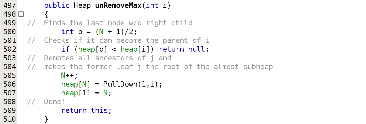
that undoes the effects of any given operation that produced a given heap . More specifically, takes a heap on nodes and an index of its node 3535 35 The presumed patch used by called by the that the presumably undoes. that satisfies the constrain
| (45) |
and produces a3636 36 The, as the Uniqueness Lemma 4.2 page 4.2 states. heap
| (46) |
on nodes that satisfies these two constrains:
| (47) |
and
| (48) |
The constrains (47) and (48) are self-explanatory. The constrain (45) is an input constrain for and needs a comment. It allows , line 506 of the Java code visualized on Figure 5, to make a child, in heap , of the first node of heap without the right child. This, for any and that satisfy the constrain (45), assures the existence of that satisfies constrains (47) and (48). If was produced by that used as the patch then, of course, (45) is satisfied. In the case of (the said node without the right child is the patch), this constrain reduces to a tautology . In the case (the left child of the said node without the right child is the patch), is even and the constrain reduces to , true for every heap on nodes. These, for any , assure the existence of index in that satisfies the constrain (45).
The and , whose existences have been demonstrated above, are unique, as the following Lemma states.
The Uniqueness Lemma 4.2
.
Proof. (i) The existence of such a heap follows form the foregoing discussion. Now, suppose that heaps on nodes and its substitute satisfy (46) and (48). Let be the path (from the root) to . Obviously, is a path in all three heaps, , , and . Since does not modify its explicit argument ( or ) except for the elements at indices along path , I infer that for every index in with ,
that is,
| (49) |
Also, by virtue of constrain (47)
| (50) |
Let , that is, be an ancestor of . We have:
| (51) |
Also
| (52) |
Thus the equality (49) is also satisfied for all . Therefore,
Hence the uniqueness of .
(ii) The existence of such an follows from the foregoing discussion. The uniqueness follows from part (i) of the Lemma (already proved) and constrain (47).3737 37 Recall that any heap is a 1-1 function.
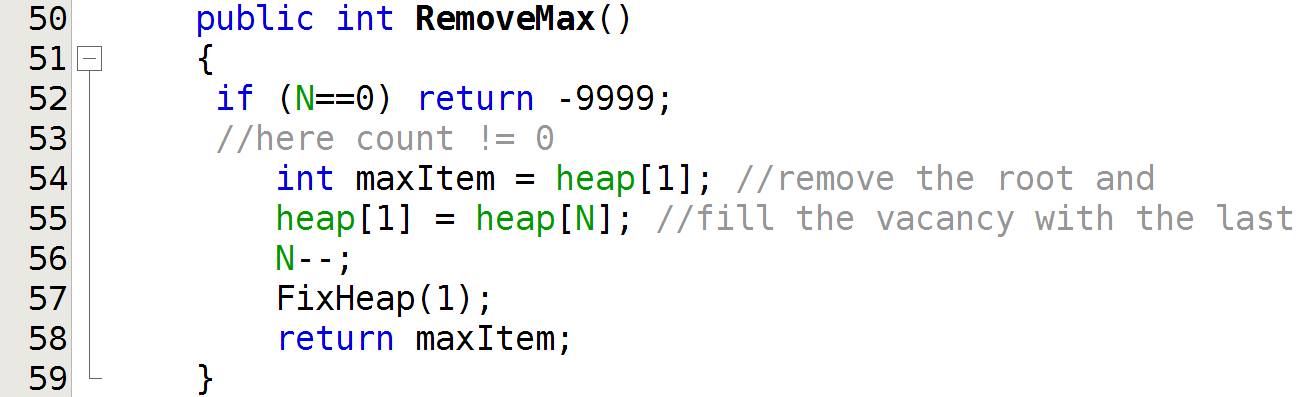
The above Uniqueness Lemma assures that the heap postulated by constrains (47) and (48) does exist and is unique. I am going to show that the Java code visualized on Figure 5 produces an -node heap out of given -node heap that satisfy constrains (47) and (48) if the constrain (45) is met; otherwise the move is invalid and returns the value as a result of execution of instructions in lines 500 and 502 of the Java code of Figure 5 page 5. Without loss of generality3838 38 Since for every heap , the result of execution of on is determined by , any two correct implementations of are functionally equivalent., I will use an example of implementation of whose Java code is visualized on Figure 6.
is a heap because is a heap, and instruction in line 507 of the Java code of Figure 5 page 5 makes its root larger than any other node of , and instruction in line 506 of that code attaches a new child to the node at index that, by asserted constrain (45), is less than , and the rest of that code does not affect the ordering of the paths in .
Constrain (47) is secured by instructions in lines 505 and 506 of the above referenced Java code. In order to show that constrain (48) is met, let us look into the implementation of operation of Figure 6.
Clearly, instructions in lines 55 and 56 of the Java code is shown on Figure 6 reverse the effects of the instructions in lines 505 and 503, as well as the effects of the assignment to in line 506 of the Java code is shown on Figure 5. At this point, the resulting tree is the same as if instruction
| H.heap[1] = H.PullDown(1,i); | (53) |
were applied to the original heap. Therefore, the Subheap Repair Lemma 4.1 applies (substituting 1 for and for ), and its part (i) implies that line 57 of the Java code is shown on Figure 6 restores the original heap. Thus constrain (48) is satisfied. As a result, and are inverses to one another, as the following Lemma states.
The Invertibility Lemma 4.3
.
Proof. (i) Let be a heap on nodes and be a heap defined by (46) page 46. Substituting (46) to (48) page 48 yields (54).
(ii) Let be a heap on nodes, be the heap defined by (48) and be the unique index whose existence is assured by the Uniqueness Lemma 4.2 (ii). Combining (46) and (48), both of which are satisfied, yields
| (56) |
or
| (57) |
The following Lemma will be useful while proving correctness of construction of worst-case heaps for .
The Cost Lemma 4.4
Proof. The only comparisons of keys within are performed by the call to in line 57 of the Java code visualized on Figure 6. Thus
| (59) |
where is the heap on nodes with for and . Since, as noted in the discussion above, performed actions that were comprised by (53), the Subheap Repair Lemma 4.1 applies (substituting 1 for and for ) and the equality (32) of its part (ii), taking into account equality (59), yields (58).
5 Decomposition of the worst-case analysis of
It is easy to generate worst-case input arrays of arbitrary size for . A Java code presented and proved correct in Appendix A of [10] does just that. However, efficiently3939 39 As opposed to, say, exhaustive search. generating worst-case heaps for and worst-case input arrays for the entire , except for some special sizes, have been, to my best knowledge, unknown. Moreover, although the sum of upper bounds of program’s components is an upper bound on the running time of the entire program, the converse is not necessarily true. For instance, for an upper bound on the number comparisons of keys performed by on an -element heap is less than the sum of any upper bounds on numbers of comparisons of keys performed by the sequence of es that comprise it. And this singularity4040 40 This singularity is characterized by Theorems 10.13 and 10.14 page 10.13. is one of the reasons why the worst-case analysis of is not totally a routine task.
Fortunately, the problem of generation of worst-case inputs for can be decomposed on two subproblems: how to, given any , generate a worst-case heap of size for , and how to, given a heap , generate a worst-case array for that converts onto . Clearly, solving those subproblems in that order will result in a worst-case array of size for . Careful evaluation of the number of comparison of keys performed on the resulting array will allow me to derive the exact formula for .
The mentioned above decomposition property implies that any upper bound on the number comparisons of keys performed by on an -element array is equal to the sum of upper bounds on numbers of comparisons of keys performed by that and on an -element array and an -element heap, respectively. In particular, the least upper bound is equal to such a sum, thus yielding
| (61) |
Based on the above observations, in order to prove (61) it suffices to demonstrate that, given a heap , the Java loop statement visualized on Figure 7 constructs a worst-case input array for the , that is, an array that the will convert onto while performing the maximum possible number of comparisons. The equalities (31) and (34) of the Subheap Repair Lemma 4.1 (i) and (iii), page 34, via constrains (43) and (44), page 43, they entail, make the latter a routine exercise.

Figure 8 shows an output generated by my Java program containing the above code.
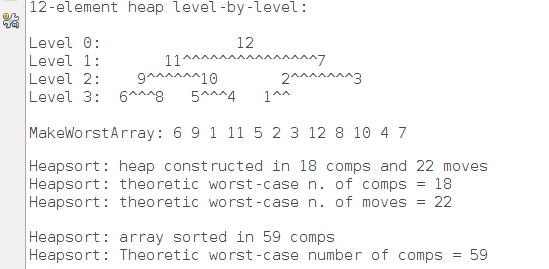
First, I will prove, by induction on , that for every , that the following program :
| for (int i = N/2; i <= K; i++) unFixHeap(i); | (62) | ||
| for (int i = K; i >= N/2; i--) FixHeap(i); | (63) |
leaves the heap , on which it is run, unchanged, that is,
| (64) |
where is the value of after the execution of on it, and that the line (63) in forces the to perform the total of
| (65) |
comparisons of keys.
If then program performs no actions, so that the invariant (64) is satisfied, and the numbers of comparisons done by the is 0, which is equal to the right-hand side of (65).
If then program is functionally equivalent to:
| for (int i = N/2; i <= K-1; i++) unFixHeap(i); | (66) | ||
| unFixHeap(K); | (67) | ||
| FixHeap(K); | (68) | ||
| for (int i = K-1; i >= N/2; i--) FixHeap(i); | (69) |
By (43) page 43, line (68) cancels out the effects of line (67), and by the invariant (64) of the inductive hypothesis, line (69) cancels out the effects of line (66). So, program leaves the heap it is run on unchanged and the invariant (64) is satisfied.
By (44) page 44, putting , the number of comparisons of keys performed by in line (68) is equal to
| (70) |
and by the inductive hypothesis, taking into account that line (68) cancels out the effects of line (67), the number of comparisons of keys performed by in line (69) is equal to
| (71) |
so that
or (65).
| (72) |
This completes the inductive proof of (65) and the invariant (64).
Since for every , is a lower bound on the number of comparisons that performs on any -element array and is an upper bound on , I conclude from (72), putting , that for every , is the least upper bound on , that is,
| (73) |
Thus, for every heap , the Java loop statement visualized on Figure 7 constructs a worst-case input array for the that converts onto 4141 41 In other words, every heap is a worst-case heap to build for the .. Hence, the equality (61) holds.
By virtue of Theorem 7.1 in [10],
| (74) |
where is the sum of all binary digits of and is the exponent of in the prime factorization of . Thus the array produced by the Java loop statement visualized on Figure 7 run on any heap of distinct elements, when given as the input to forces it to perform comparisons of keys and to yield the heap .
Note. The sequence of integers
given by the formula (74) and visualized on Figure 9 appears as the Sloan sequence A092054 in [1].
At this point it becomes clear that all that is needed for the completion of the worst-case analysis of is a derivation of a formula for the worst-case number of comparisons of keys performed by the RemoveAll. I will do just that in the sequel of this paper.
6 The game of Pull Downs
Both and have nice worst-case decomposition properties that allow to compute their worst-case numbers of comparisons of keys as sums of worst cases of their components. Unfortunately, the same cannot be said of . Although, for arrays of size less than or equal to 12, the worst-case number of comparisons of keys performed by is equal to the sum of the worst-case numbers of comparisons of keys of the ’s that make , it is not the case for arrays of more than 12 elements4242 42 As I have indicated at the begining of Section 5 page 5; see footnote 40.. In the latter case, the worst-case number of comparisons of keys is performed by is always less than the sum of the worst-case numbers of comparisons of keys of the ’s that make .
In order to construct worst-case heaps for and prove that they actually are worst-case heaps, I will resort to games and strategies.
Imagine the following solitaire game played by the Player.
A game is a sequence of heaps in which is the one-element heap whose only node is ,4343
43
Formally, , so the only node of is ; naturally, it is identified by its value 1 (the second element in the pair). and for every positive integer , heap is the result of a valid application of the operation , visualized on Figure 5 page 5, to heap . In particular, each is a heap on nodes.
Each application is an -th move, and I will refer to it in some contexts as a pull down4444
44
A call to method , visualized on Figure 3 page 3, is part of method ; hence the name pull down.,4545
45
The reason for using both moves and pull downs is to simplify notation. For instance, it allows using pull down (on a heap ) in lieu of move .
if it is a valid application, that is, if the instance
of the constrain (45) is satisfied.
The Player draws at random an integer and executes a sequence of consecutive4646 46 The adjective consecutive in this context means that each next pull down of the said sequence is applied to the heap produced by the foregoing pull down. pull downs on the 1-element heap . The result is an -element heap . Player’s goal is to maximize the payoff for the game defined as the number of comparisons of keys that the ’s reconstruction phase will perform while run on the heap .
Given a game , its every -th move is determined by the index , and the game itself is determined by the sequence of indices that are the arguments of respective ’s. Thus there is a function between the sequences of valid moves and games that is defined by:
| (75) |
Because of that, I will identify moves with their arguments . Also, since I assumed (on page 15) that any heap is a function, and as such has the inverse , any index in is unambiguously identified by the node that is stored at . Thus the game is also determined by the sequence
| (76) |
of patches where is the argument of respective , simply because the sequence in (75) is determined by
| (77) |
This fact allows me to identify pull downs with patches (the values that are being pulled down) rather than with their indices. For instance, given a heap , pull down 6 is the move .
I will also consider finite subgames of game that I define as finite sequences of heaps from . Clearly, any finite subgame is determined by the heap and the subsequence of of valid moves. This gives rise to function defined by
| (78) |
As before, given heap , any finite subgame is unambiguously determined by the corresponding subsequence
| (79) |
of pull downs applied consecutively46 to , simply because the sequence in (78) is determined by
| (80) |
For example, if the subsequence of pull downs is equal to then the corresponding subsequence of moves is equal to:
| (81) |
Given heap , each of these subsequences will serve as a definition of the last heap in the subgame . For instance, one can verify (a program can do it) that given the 1-element heap , the sequence of pull downs , and the sequence of moves , define the 7-element heap visualized on Figure 11.
Since is a function4949 49 is not a function since the range of its restriction to -element heaps has a lesser cardinality than its domain., pull downs of two different patches and (for instance, pull down 1 and pull down 2) produce different heaps regardless whether they were applied to the same heap or not. For if both pull down and pull down produce the same heap , then the heap that they were applied to is given by and, therefore, is unique, and so is the patch that was used to fill the vacancy after the largest element of was removed. Thus, . Hence, different sequences of consecutive pull downs are never coalescing5050 50 So that the graph of the game of Pull Downs is a tree. in that they always produce different heaps from their residua no matter what the heaps are5151 51 As long as all moves in the said sequences are valid.; a routine induction argument yields the proof. As a result, different games are never coalescing as well5252 52 Thus heaps and games form trees of sequences whose property of never coalescing implies the uniqueness of the path (from the root) to any given node..
In particular, every heap has the unique sequence of consecutive pull downs which produce it (, that is) from the heap .5353 53 The sequence can be constructed via the equality (79), where is the reversed sequence of consecutive residua of the heap .
Thus there is a correspondence between all heaps and sequences of valid applications of . In particular, the number of different heaps of size is equal to the number of different sequences of patches5454 54 Recall that not every node can serve as the th patch since its index must satisfy an instance of inequality (45) for ..
The above observations prove the following Theorem that will allow me to reduce the worst-case analysis of to analysis of some winning strategies for the game of Pull Downs.
The Mapping Theorem 6.1
For every heap of nodes and its residue of nodes, there is a unique sequence of consecutive pull downs that produce from ; in particular, there is a unique sequence of consecutive pull downs that produce from the 1-element heap.
Proof follows from the above discussion.
I will call the unique sequence of pull downs mentioned in Mapping Theorem 6.1 a creative sequence of relative to and denote it by . In the case of bring the 1-element heap , will I call it simply a creative sequence and use notation in lieu . By Mapping Theorem 6.1, for any , is a function of and, therefore, has the inverse . I will denote it by , or, in the case of , by .
Thus is the sequence of pull downs that result in heap when applied consecutively to heap , and is the heap created by application of the sequence of consecutive pull downs to the heap .
It follows from the above definitions that is a residue of if, and only if, is an initial proper subsequence of 5555 55 Formally, if and .
7 Credits for moves
I define credit for a move applied to a heap on nodes to be equal to the number of comparisons of keys that application of operation to a heap produced by will perform. By the RemoveMax Cost Lemma 4.4 page 4.4, it is given by the equality (58) page 58. It is a function of and the number of nodes of .
The equation (58) page 58 can be rewritten to a human-readable form as follows, substituting for and for .
If is an index of a leaf with a sibling then
| (82) |
and, by (32),
| (83) |
One can verify by means of direct inspection that in this case the right-hand side of the equation (83) also yields the credit for pulling down the parent of the node at index , that is,
| (84) |
If is an index of a leaf with no sibling then then
and, by (32),
| (85) |
As before, the right-hand side of the equation (85) also yields the credit for pulling down the parent of the node at index in this case, so
| (86) |
Also,
| (87) |
Since , defined by
| (88) |
is, by virtue of the definition of at the beginning of this Section, equal to the maximum number of comparisons of keys that the may perform on any heap on nodes5656 56 In particular, the heap produced by a pull down applied to a heap on nodes., application of the equality (60) page 60 yields
| (89) |
The loss of credit relative to the said maximum for a move in a heap on nodes is defined as:
| (90) |
If then the move and the pull down that yielded the credit are called lossless; otherwise, they are called lossy.
The following Lemma characterizes lossless moves.
Credit Loss Characterization Lemma 7.1
Let be a heap of nodes and let be a valid move (that is, one that satisfies the inequality (45) page 45). Move is lossless if, and only if, one or more of the following conditions are true:
- (i)
, or
- (ii)
, or
- (iii)
is a sibling node5757 57 Formally, . in the last level 5858 58 Formally, . of , or
- (iv)
is the parent of a sibling node5959 59 Formally, . of the last level 6060 60 Formally, . of .
Proof First, I will prove the if part of the Lemma.
(iii) Since belongs to the last level of , . Thus, by equality (83) page 83,
[by equality (89)]
Thus,
Hence, by the equality (90),
(iv) has a similar proof except that it begins with the equality (84) page 84 rather than with (83).
(i) Since , belongs to the last level of , therefore is a leaf in that level. If has a sibling then the case (iii) applies, which completes the proof of this case. If has no sibling then its parent has one child only, that is
Thus
Hence,
that is,
| (91) |
[by equality (91)]
Thus,
Hence, by the equality (90),
(iv) follows from (i) by virtue of equality (84), in the case has no sibling, or equality (84), otherwise. This completes the proof of the if part of the Lemma.
If is neither a leaf nor the parent of a leaf, which means that , then, by the equality (33) page 33,
| (92) |
By virtue of equality (32) page 32,
| (93) |
and
Thus
| (94) |
Subtracting (93) from (94), we get
Hence, by (92),
and, therefore,
thus making a lossy move.
If is a leaf but not in the last level of then , so, by virtue of equality (32) page 32,
Thus
and, therefore,
thus making a lossy move.
If is a parent thereof then, by virtue of equality (84), in the case has no sibling, or equality (84), otherwise,
and the same conclusion as for the previous case follows.
Since there are no other cases, this completes the prof of the only if part, which completes the proof of the Lemma.
One can immediately conclude from the above Credit Loss Characterization Lemma 7.1 (i) that for every , there is a heap of nodes and an index such that pull down yields the maximum credit 6161 61 For instance, pull down 1 in a heap of nodes that satisfies the equality yields the maximal credit ., turning the inequality (88) into equality for such , , and , and, therefore, making that inequality tight for every .
Function will allow me for easy evaluation of payoffs for some strategies.
Let’s consider for example a sequence of alternating pull downs applied consecutively to a complete heap on nodes. If then both moves are valid and lossless. For , since nodes 1 and 2 are the smallest nodes in any heap on N nodes, all these moves are valid as well, that is, the inequality (45) page 45 is satisfied for every and . It turns out that in the latter case, all these moves are also lossless, except, perhaps, for the second move that may lose 1 credit to , as one can conclude from the following Lemma.
The pq Lemma 7.2
Let be a complete heap on nodes, let , with , be its leaves, and let , where , be a sequence of pull downs of and , applied consecutively to , that is given by this regular expression
| (95) |
- (i)
All moves of , except, perhaps, for move , are lossless.
- (ii)
If then move is lossless.
- (iii)
If then move loses credit relative to the maximum for that move.
Proof. Let 6262 62 Function was defined by (78) page 78. be the sequence of heaps produced by pull downs applied to .
Move (the first move in the described sequence) pulls down , which resides in the last level of as a leaf with a sibling, down to index in . By the Credit Loss Characterization Lemma 7.1 (iii), move is lossless, with
| (96) |
Move pulls down , which either resides in at index as the parent of (that has been pulled down to index by move ) or as a leaf with a sibling. In the latter case, it scores the same credit as move did, that is,
[since and, therefore, ]
Thus,
| (97) |
This, by (89) and by inequality (88) on page 88, yields one less than the maximum of credit for any , thus making move lossy, with
| (98) |
This completes the proof of case (iii).
In the former case ( resides in at index as the parent of its only child ), move pulls down . By the Credit Loss Characterization Lemma 7.1 (ii), move is lossless, with
This completes the proof of case (ii).
Moves and , where pull down and , which reside in level of heaps and as leafs with siblings. By the Credit Loss Characterization Lemma 7.1 (iii), each of those moves is lossless, with
I will use special cases of sequences , namely, , in establishing some important constrains on optimal strategies, and later in Section 10, , in design of an optimal strategy for the game of pull downs.
8 Strategies and their payoffs
A strategy is an infinite sequence of valid moves consecutively applied to the 1-element heap . Given a strategy , I will call the sum of the the credits, defined in Section 7 page 7, for all moves of between -th and -th move6363 63 Racall that move of any strategy produces an -element heap out of an -element heap, inclusively, where , the the payoff . It is given by this formula:
| (99) |
The following lemma shows that the payoff for the game, defined on page 6, that the Player plays with a strategy is equal to the payoff for the strategy .
The Cost Lemma 8.1
Let be a heap of nodes and be its creative sequence.
| (100) |
Proof by induction on . For , both sides of (100) are 0, which observation completes the basis step.
Let (100) be true for some , be a heap of nodes, be its creative sequence, be the heap produced by execution of , and be the creative sequence for . By the above definition of ,
| (101) |
By the definition of creative sequence at the end of Section 6 on page 6, . Since has nodes, by the inductive hypothesis we get
| (102) |
Substituting (102) to (102), we obtain
[by the definition of credit at the beginning of Section 7 page 7]
which yields (100), thus completing the inductive step.
If and then all moves between -th and -th move, inclusively, construct the level of the output heap. In such a case, both the argument of the -th move and the result of the -th move of are consecutive6464 64 The difference between their depths is equal to 1. complete heaps; I will call the payoff , given by the equality (99), a level payoff and denote it by . Formally,
| (103) |
Informally, it is the sum of credits of moves of that added the next level to the complete heap 6565 65 Function has been defined on page 6. on nodes created by the first moves of consecutively applied to the 1-element heap .
Similarly, I will call the sum of the the losses for all moves of between -th and -th move, inclusively, where , the the accumulated loss . It is given by this formula:
| (104) |
where
| (105) |
with abbreviated notation
| (106) |
that yields
| (107) |
If then I call the sequences of moves and of pull downs of lossless; otherwise, I call those sequences lossy.
The level loss at level is given by this formula:
| (108) |
If then I call the level lossless; otherwise, I call it lossy.
It follows directly from the definition (108) that for any natural number :
| (109) |
If is the size of the largest complete heap of no more than nodes and is the depth of that heap then
[by (109), taking into account that ]
[by virtue of equalities (24) and (25) page 25]
Thus, for any
| (110) |
If, moreover, then and , so that , and (110) reduces to
| (111) |
If is a residue of heap then the payoff earned by the creative sequence 6666 66 Function defined on page 6. is given by:
| (112) |
where and are the sizes of heaps and respectively. If is the 1-element heap then I will use as an abbreviation of . By the equality (100) in the RemoveAll Cost Lemma 8.1 page 8.1,
| (113) |
where is the number of comparisons of keys performed by the execution of on heap . Thus,
| (114) |
where is any strategy whose st move produces heap and -st move produces heap .
Under the same assumptions as above, the accumulated loss (of credits) for the creative sequence is given by:
| (115) |
If is the 1-element heap then I will use as an abbreviation of . on heap . Thus, by (104), it satisfies this equality:
| (116) |
where is any strategy whose st move produces heap and -st move produces heap .
I will call the payoff yielded by the sum of credits that match the maximum given by (89) page 89 for all moves of between and , inclusively, where , the upper-bound payoff. It is given by this formula:
| (117) |
For any heap on nodes and its residue on nodes we have:
As a special case of (117), we have:
| (119) |
which, by virtue of equality (20) in [10], yields:
| (120) |
Thus is and upper bound for .
| (121) |
Equation (121) will allow me for easy derivation of the value of payoff from its upper bound , given by a known closed-form formula, once I have computed the loss of credit .
Thus the Player draws at random an integer , choses any strategy , and plays the first moves of it. By the definition of Player’s payoff on page 6, his total payoff is equal to the number of comparisons that will perform while run on the heap 6969 69 The function has been defined on page 6. produced by the st move of the strategy . This, by virtue of the definition (99) page 99 of and the Cost Lemma 8.1 page 8.1 is equal to
| (123) |
His total loss of credit, defined as
| (124) |
determines whether the strategy he choose is optimal, according to the following Lemma.
Lemma 8.2
A strategy is optimal for if, and only if, for every strategy ,
| (125) |

The Player wins if the payoff for the strategy he choose is optimal, that is, cannot be beaten by any strategy for the same .
Theorem 8.3
A strategy is optimal for if, and only if, its first moves produce a heap 69 that forces to perform the worst-case number of comparisons of keys.
Proof. Suppose that is an optimal strategy for but the heap is not a worst-case heap for . In such a case, Player can pick up an -element worst-case heap for , run on it while recording a sequence of patches that were used to fill the vacancies left by the removed maximal elements, and then play any strategy whose first moves are given by the reversed sequence . Since the payoff for the Player , by the definition (32) of page 32, is equal to the number of comparisons performed by , and the payoff for the Player is, equal to the number of comparisons performed by , the payoff for the Player is larger than the payoff of the Player , and so the Player wins, contrary to the assumption that the Player had an optimal strategy for .
The player could try to apply a brute force and devise a greedy strategy that maximizes credits for its all moves. This could be done relatively easily with a program that attempts to generate a greedy substrategy for any given size of a worst-case heap. Unfortunately, as I illustrate in B page B, any such greedy substrategy must fail to produce any worst-case heap of more than 22 nodes.
In the next Section, I will use a bit subtler approach to generation of worst cases for .
9 Strategies and , and the lower bounds they establish

Given an integer , I will construct an optimal strategy for that . For , one can take any worst-case heap of nodes7070 70 Beginning with a worst-case heap on nodes and using heaps of nodes as benchmarks, instead, would be, perhaps, more rational but it would also make the their illustration on Figures 11 and 12 less neat. (for example, the heap visualized on Figure 11) and extract its creative sequence of the first pull downs (for example, the creative sequence for the heap , given by the first 6 moves of the sequence shown in A.1 page A.1) of a strategy from it; we will see in a moment that (e.g., ), where is an infinite7171 71 Just to make the entire sequence infinite. sequence of pull downs, for instance, , is an optimal strategy for every . Some straightforward experimentations with different sequences of pull downs allow one to find optimal strategies for (for example, is such an optimal strategy the first 11 moves of which produce a 12-node worst-case heap visualized on Figures 1, 2, and 8 pages 1 and 8; see A.1, page A.1 for details of construction of such a heap).
For , such a construction of is easy if the sought-after worst-case heap is complete, that is, if ; the mentioned above sequence followed by any infinite sequence of pull downs that makes their concatenation ’s level loss for every (for instance, followed by the infinite sequence of alternating pull downs of 1 and 2) will do. However, showing that such a construction results in an optimal strategy for any is nothing but a routine exercise due to the number of cases to consider in order to carry on the proof of it7272 72 See [6] for an example of such a proof..
If then the construction of an optimal strategy, although still relatively simple7373 73 FIX THIS A combination of the strategies and , is, perhaps, a bit harder to discover; its detailed proof7474 74 At least the one I know. is definitely convoluted.
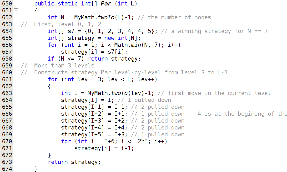
I begin with constructing the base strategy , whose Java code is shown on Figure 13, that is an optimal strategy for every (in particular, for ), but not for any other .
The 7th heap in the game carried on with strategy is visualized on Figure 11. As I have indicated, the creative sequence for is . Thus, by (81) page 81, the first six moves of are .

One can easily verify (a program or an argument will do) that application of operation to performs 14 comparisons of keys, which number happens to be equal to the known7575 75 See, for instance, [10] for a proof of the formula for any heap on (not just on ) nodes. upper bound
on the number of comparisons of keys that the performs on any heap of 7 nodes. Thus 14 is the worst-case number of comparisons of keys that the performs on any heap of 7 nodes, and, therefore, is a worst-case heap for .
The heaps through of are defined as the residua of successive applications of to . The creative sequences of those residua are the beginning subsequences of the creative sequence for . Because
| (126) |
where is the maximum number of comparisons of keys that the performs on any heap of nodes, those creative sequences are lossless. As a result all the residua of , that is, the heaps through , are automatically worst-case heaps for and, therefore, for .
After the 7th move, the strategy is defined inductively level-by-level. For any with,
| (127) |
it takes the heap on nodes, whose scheme is visualized on Figure 12 (for instance, heap of Figure 11 falls under that scheme), that it has constructed so far, and adds to it the next level by performing on a sequence of consecutive moves such that the resulting heap on nodes falls under the scheme of Figure 12 and all these moves are lossless except for one move (the second move in the described sequence) that scores a credit that is one less than the maximal score.
More specifically, move (the first move in the described sequence), implemented by the statement at line 664 in the method shown on Figure 13, pulls down 1 that resides at index of heap . That move, among other effects, brings node 3 to the last index in the level of and makes node 1 the child of node 4 at index . Nodes 2 and 4 maintain their indicies and , respectively, in heap .
Move , implemented by the statement at line 665 in the method shown on Figure 13, pulls down 2 that resides at index of heap . Nodes 3 and 4 are not affected because they reside at the same level as 2 did in .
Move , implemented by the statement at line 666 in the method shown on Figure 13, pulls down 1 that resides at index of heap . That move, among other effects, brings its parent 4 to the first index of the last level of of . Nodes 2 and 3 are not affected.
After that, the remainder moves , implemented by the statements at lines 667 through 672 in the method shown on Figure 13, keep pulling down 1 and 2 that reside as leaves in heaps , making sure that they always pull down a node with a sibling, and that the two last moves are pulling down 2 and then 1. Nodes 3 and 4 are not affected by any of those moves, except that node 3 becomes the parent of node 2 in and the parent of nodes 1 and 2 in .
Obviously, all the moves are valid because no other node of any heap is smaller than 2 and 1.
The resulting heap falls under the scheme of Figure 12; the first node in the last level of is 4, the last two nodes and in the last level of are 2 and 1 in that order, and the parent of 1 and 2 in is 3. Moreover, by the pq Lemma 7.2 (i) and (iii) page 7.2 substituting 1 for and 2 for , taking into account that , all the moves were lossless, except for the th move (the second move in the sequence of the pq Lemma 7.2) that scored a credit one less than the maximal credit for the st move.
This way we proved the following two theorems.
Theorem 9.1
Every heap on nodes, where , produced by strategy satisfies the invariant visualized on Figure 12.
Proof follows from the above discussion.
Theorem 9.2
For every ,
| (128) |
Proof. If then because the first 6 moves of strategy are lossless. If then, by (126), for all except in the above discussion, that is, , for which .
Figure 14 shows a graph of .
A Java code that implements strategy is shown on Figure 13, and an example of a heap produced by strategy is shown on Figure 15. The subsequence of the first 14 moves of that produced it is:
and the sequence of corresponding pull downs is:
The sequence of 14 heaps created by these moves is shown in the A.1 page A.1.

Let for every , the delayed loss function be defined by:
| (129) |
I will show in Section 10 that function establishes a lower bound on accumulated loss of credit for moves through for any strategy. The following Lemma provides a closed-form formula for that lower bound.
Lemma 9.3
For every ,
| (130) |
Proof. By virtue of definition (129), is equal to the number of ’s that are less than or equal , with , or . Since is a function, that number is the same as the number of different values of between 4 and , which is equal to for (same as ) or otherwise.
Graphs of functions and are visualized on Figure 16.
Lemma 9.4
For every , the following equality holds:
| (131) |
Proof. The least solution of the equation
| (132) |
that occurs in (129) is , so for . Thus for . Since, by (128), for , also [by the equation (108) page 108] for . Hence (131) holds for .
For each , the equation (132) has exactly one solution that satisfies , namely, , and so does the equation that occurs in (128), namely, . Thus both , that by (108) is equal to , and are equal 1. Hence, by (108), the equation (131) holds for each .
Lemma 9.5
For every , the following equality holds:
| (133) |
Proof. By the equality (109) page 109,
[by the equation (131) in Lemma 9.4]
[since ]
Hence, (133) holds.
Figure 17 visualizes graph of function .
Not surprisingly, it coincides with function for some , as the following Lemma states.
Lemma 9.6
For every , the following equality holds:
| (134) |
Proof. If then the equation (134) follows from (134) since
If and then
| (135) |
and
| (136) |
Thus
[by (135)]
[by (136) and the already proven case of (134) for ]
Hence, (134) holds.
The about facts about strategy is all I need to derive and prove the main results of this paper. Below is its more definitive characteristics that I quote here for an illustration.
The payoff after moves of the strategy for is given by this formula:
| (137) |
Figure 18 shows a graph of the total payoff function for . Of course, , given by (137), is a lower bound for the number of comparisons of keys that performs in the worst case on an -element heap.
The strategy loses 1 credit per level, beginning with level 3, and in the very second move of each such level. Thus switching to a greedy strategy in the last level of the produced heap (moves through , provided that ) may help one to avoid the loss of credit in the last level and, therefore, result in a set of strategies that are better than for infinitely many .
It turns out that, given , a strategy that is a combination of the strategy , played for all levels from 0 to , and a greedy7878 78 One that does not admit any delayed gratification, that is, takes a loss only if no lossless move is valid at the moment. strategy for the level if , is an optimal strategy for , that is, it produces a worst-case heap in its first moves. I am going to show that for every , the above arrangement allows to postpone the loss at the move , that the strategy would have to incur, up until the move of if , or avoiding that loss altogether, otherwise. In the latter case, for all , strategy will beat by 1 credit after completion of their first moves. This fact and the formula (137) for will yield the formula for payoff for strategy .
I define the greedy strategy that in the case of
| (138) |
is played in the last level [by (138)] of the constructed heap as follows:
- (i)
It pulls down 1 (the last element of the heap of nodes that is shown on Figure 12).
- (ii)
It pulls down 4 (the new parent of 1).
- (iii)
- (iv)
It pulls down 1.
- (v)
It pulls down 1 and 2.
- (vi)
After that, it keeps executing pull downs of 1 indefinitely (just to make an infinite sequence)
More specifically, is defined inductively level-by-level, from level 3 up. For any that satisfies inequality (138), it takes the largest complete heap of no more than nodes, which by (24), happens to have
| (139) |
nodes, that was created by the first moves of and, therefore, by virtue of Theorem 9.1, falls under the scheme visualized on Figure 12, and performs on it a sequence of consecutive moves as follows.
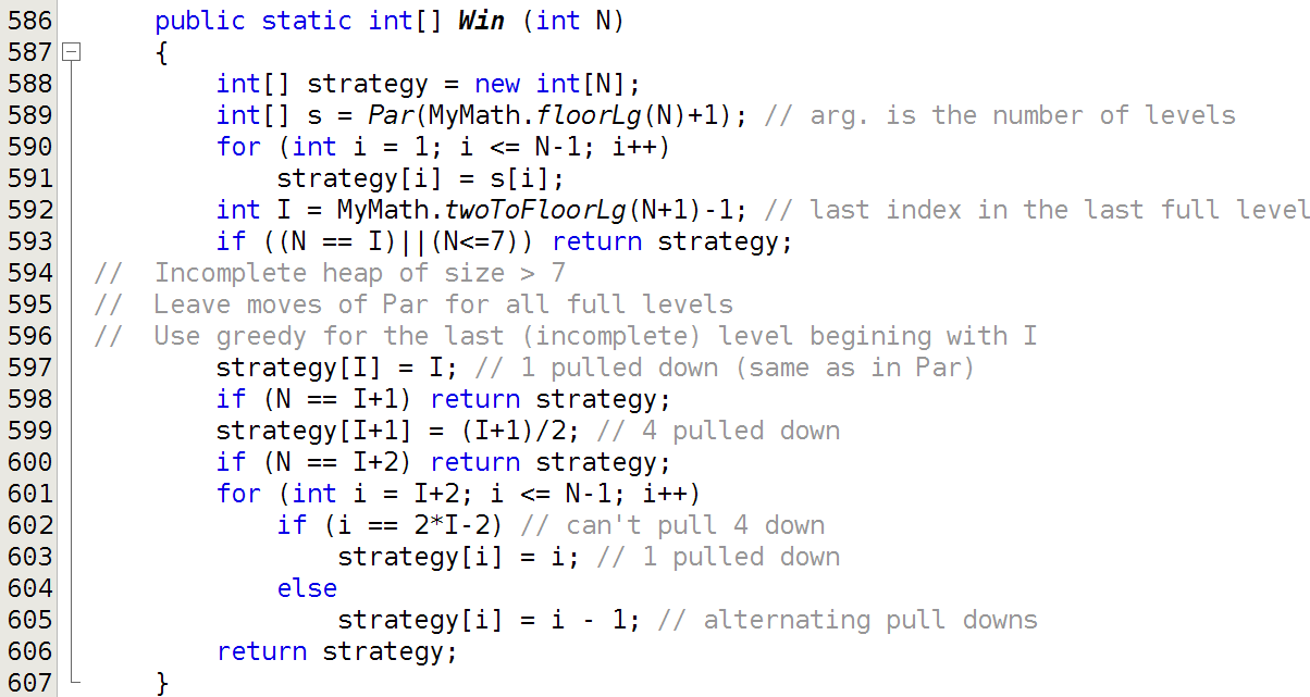
The move (the first move in the described sequence), implemented by the statement at line 597, with computed by the statement at line 592, in the method shown on Figure 19, pulls down 1. That move, among other effects, brings node 3 to the last position in the level of and makes 1 the only child of 4.
The move (or ), implemented by the statement at line 599 in the method shown on Figure 19, pulls down 4.
After that, the moves , implemented by the first part of the -loop where (the statements at lines 601 through 606) in the method shown on Figure 19, keep pulling down 1 and 4 that reside as leaves in heaps , making sure that they always pull down a node with a sibling. All those are valid moves since 1 is the least node in any heap and the only two nodes 2 and 3 that are less than 4 reside at the last two indicies and of level in heaps .
If is not done at this point, that is, if , then the move , implemented by the statement at line 603 in the method shown on Figure 19, pulls down 1, which resides in as the parent of 1 that is a leaf at index and has no sibling. So, it scores the same credit as move that pulled down 4 for the first time did, that is,
[by virtue of (127)]
This, by (89) and the inequality (88) on page 88, yields one less than the maximum of credit for any , thus making move lossy, with
| (140) |
After that, if is still not done, that is, if , then the reminder move , implemented by the statement at line 605 in the method shown on Figure 19, pulls down 2 that resides as a leaf with siblings in heap . By the Credit Loss Characterization Lemma 7.1 (iii) page (iii), move is lossless, with
At this point, , that computes only the first moves of , terminates because , so the next move after the move would fall beyond that range.
Obviously, the last two moves are valid because no other node of any heap is smaller than 1 and 2. Moreover, by The pq Lemma 7.2 (ii) and (iii) page 7.2 substituting 1 for and 4 for , taking into account that , all the moves up to and including the move were lossless. Thus, since , all the moves between and were lossless, except for move that scored a credit one less than the maximal credit for st move.
This way I proved the following theorem.
Theorem 9.7
For every ,
| (141) |

N = 14
 N = 30
N = 62
N = 30
N = 62
Proof Follows from the above discussion. In particular, the equality (141) can be easily extracted from the code of Java program shown on Figure 19 page 19.
Since for , is an optimal strategy for . Thus the heaps created by the first 11 moves of are all lossless and, therefore, worst-case heaps. Hence, all worst-case heaps of 12 nodes or less are lossless, too.
I am going to prove in Section 10 that for every (not just for ), is optimal for .
Lemma 9.8
Proof. By (129) page 129, for , if, and only if, , the latter of which, by (141) page 141, holds for if, and only if, . Thus,
so that
Therefore, since
in order to prove (142) it suffices to show that
| (143) |
Since by (141) page 141, for all , ,
[by the equality (133) in Lemma 9.5 page 9.5, substituting for ]
This completes the proof.
A Java code that implements the strategy is shown on Figure 19. A worst-case heap on nodes produced by the strategy and the sequence of the first pull downs of , which is the same as the sequence of the first pull downs of , is shown on Figure 21. The sequence of 14 heaps created by the last 14 of these moves is shown in the A.2 page A.2.
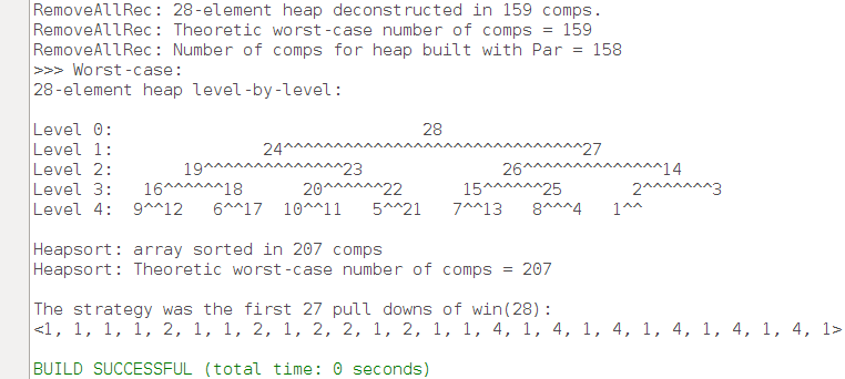
Now, we are ready to compute the accumulated loss for each strategy .
Lemma 9.9
For every ,
| (144) |
Proof. By the equality (142) in Lemma 9.8 page 142, . Application of Lemma 9.3 page 9.3 completes the proof.
A graph of function is shown on Figure 22.
The Lower Bound Theorem 9.10
The payoff after moves of the strategy for is given by this formula:
| (145) |
where is a binary function on the set of integers defined by:
| (146) |
Function is visualized on Figure 23. It raises from 0 to 1 when the strategy performs a lossy move in the level , and drops from 1 to 0 when the strategy performs a lossy move in that level.
Proof. Since, by (121) page 121, , by virtue of (144), it suffices to prove that for any , (145) is equal to
| (147) |
Once we pinpointed correct formulas, verification of that equality is easy.
If then , , and so that (145) reduces to:
and so does (148). Thus (145) and (148) are equal in this case.
If then , and , so that (145) reduces to:
| (149) |
and (148) reduces to
| (150) |
Thus, in order to show that (145) is equal to (148) it suffices to show that (149) is equal to (150), or, subtracting the common term from (149) and (150), to show that
that is,
or, incorporating the definition (146) of ,
| (151) |
I will show that for every , (151) holds.
Indeed, if then . So, , that is, . Thus . Hence, since is a non-decreasing function, and , thus proving (151) in this case.
If, however, then and . Thus . Hence, and, since for , , , thus proving (151) in this case, too.
Since there are no other cases, this completes the proof of (151).
10 The proof of the winning
Granted the optimality of for each , all heaps produced by are worst-case heaps as long as the corresponding pull downs are lossless. If no greedy strategy exists that would perform more consecutive lossless pull downs on any worst-case heap on nodes than does on the worst-case heap then, taking into account that, by virtue of the equality (141) page 141, loses no more than 1 credit relative to in the entire th level, all heaps produced by are worst-case heaps, thus making the combination an optimal strategy for .
So, the basic question that needs to be answered in order to decide the optimality of for is how many consecutive lossless pull downs a worst-case heap on nodes may admit. I am going to show that no more than , that is the same as does admit on the heap . From that the optimality of for will follow.
If then pulling down 1 yields credit, which is maximal, so it implements the desired lossless strategy for the level .
If then pulling down 1 twice or pulling down 1 and then pulling down its new parent yields credit, which is maximal, so it implements the desired lossless strategy for the level .
If then the first two pull downs in the last level determine the maximum credit that the best greedy strategy in that level can collect.
Let and be the first two nodes that ended up in the last level as a result of the first two pull downs. (In the example of strategy for , it would be 1 and the first node in level after the strategy was executed.)
Consider heap that was produced after these two pull downs.

How far any strategy could proceed without a loss of credit relative to the upper-bound payoff ? It turns out that the index of the first node in the level of heap that is less than the maximum of and (see Figure 25) puts the limit on the number of consecutive lossless pull downs that the strategy in question can make. This intuitively obvious fact has a surprisingly unobvious proof, quite a typical sample of the fine-grain complexity of this subject matter.
Lemma 10.1
Let be a heap on nodes, where , and let and be its last two nodes. If is the index of a node in the level of heap with then heap does not admit a sequence of more than consecutive lossless pull downs.
Proof. Since , is not a parent of and , the only nodes in the last level of . So, is not a parent of or . Thus is a leaf in , and so
| (152) |
Because , the level number of , equals to ,
| (153) |
Let’s assert that the lemma is false. Let be a sequence of consecutive lossless pull downs executed on . By (152), . Let , let be the heap on nodes produced by the first pull downs of , and let be the set of all ancestors (proper and improper) of the nodes in the last level of heap , with convention . By virtue of (153),
| (154) |
Since the number of nodes of is odd, the number of nodes in the level of is even. In particular, every element of level in has a sibling in , also an element of that level.
First, I am going to show that a pair of lossless pull downs may only pull down elements of . Let , be the nodes pulled down by , respectively. For the pull down to be lossless, by the Credit Loss Characterization Lemma 7.1 page 7.1, taking into account that the last level of each heap in question has at least 2 nodes so that each of the conditions (i) and (ii) of that lemma entails the disjunction of conditions (iii) and (iv), must be a sibling of a node in the level of heap or a parent thereof. In particular, it must be an element of . For the pull down to be lossless, by the Credit Loss Characterization Lemma 7.1, must be a sibling of a node in the level of heap or a parent thereof. The only such node that can possibly be not in is the (new) parent of in , which, however, has one child only (, that is) because has an even number of elements and so its last level has an odd number of nodes, so that the last element (, that is) of the last level of cannot have a sibling. Therefore, by , by the Credit Loss Characterization Lemma 7.1, the (new) parent of in cannot be pulled down or otherwise would be lossy.
Second, I prove by induction on that for every with , the two smallest elements of are . Indeed, and are the only nodes in the last level of the heap , so , where is the set of proper ancestors of in the heap . Since no element in is less than , the two smallest elements of are . For , we have , where is the set of proper ancestors of the nodes in the last level of heap , because moves pulled down elements of . Since no element in is less than , the two smallest elements of are the same as the two smallest elements of , that is, .

Because , for any . Therefore, none of the moves of the sequence pulls down , which stays put during the execution of . Thus the last two moves and the of sequence result in attaching the (new) children , to node (see Figure 26). They must both pull down elements from the set . Since there is at most one element of that is less than and qualifies as its child, such a case is clearly impossible. This contradicts the assertion that the lemma is false.
The following technical lemma uses function of accumulated loss of credit given by the equation (115) page 115. It derives properties of some heaps and their residua from properties of virtually unrelated heaps and their residua of the same sizes as and , respectively. Although the facts spelled out by this lemma may seem inconsequential and intuitively obvious, and have elementarily-algebraic and straightforward proofs, they have allowed me to cut the lengths7979 79 By about a factor of four or so. of some of the lengthiest proofs of some fundamental results in this Section.
Diagram Lemma 10.2
Let and be heaps on nodes, and and be their respective residua on nodes. If is a worst-case heap then the following are true:
- (i)
If then .
- (ii)
If is a worst-case heap and then and are a worst-case heaps and .
- (iii)
If is a worst-case heap but is not, and then is a worst-case heap.
- (iv)
If is a worst-case heap but is not, and then is a worst-case heap and .
Proof.
Consider a differential diagram (a weighted directed graph) , an example of which is shown on Figure 27, whose nodes , , …, are heaps and weights of edges are differences
| (155) |
where is the number of comparisons of keys performed by the execution of on heap . Obviously, any differential diagram commutes, that is, any two paths in with the same source and destination have equal weights.
In particular, the diagram with heaps , on nodes each, and their respective residua and on nodes each, visualized on Figure 28, commutes.
Here is the upper bound on credit for the sequence of pull downs that produces an -element heap from and -element heap, and and are accumulated losses of credits given by the equation (115) page 115, so that
and
Let’s assume that is a worst-case heap. In such a case,
| (157) |
If then and, by (156),
that is
| (158) |
This proves (i).
If
| (159) |
then by (156)
[by (157)]
that is,
Thus if is a worst-case heap then is a worst-case heap, too. Hence,
| (160) |
By (i), inequality (158), and inequality (159)
| (161) |
By virtue of (156) and (160) and (161),
If is a worst-case heap but is not then
| (162) |
Therefore, if then (156) yields:
Since is a worst-case heap, so is . This proves (iii).
If is a worst-case heap but is not, and then, by (iii), is a worst-case heap, and so
| (163) |
Also, since is a worst-case heap,
| (164) |
that is,
[by (164)]
Hence,
that is,
This proves (iv).
The following lemma imposes rather rigid limits on how far one optimal strategy can fall behind another. It is a consequence of the existence of strategies that are lossless up until level 3 and, like the substrategy of alternating pull downs of 1 an 2, lose only one credit per level relative to their respective upper bounds 8080 80 One can directly compute for any as . Intuitively speaking, there are pull downs between and , each collecting maximal credit of , except for the first one that loses 2 credits relative to and for the second one that that loses 1. for each level , with which optimal strategies must compete in order to win.
Competition Lemma 10.3
For every worst-case heap on nodes,
- (i)
the last level of can lose no more than 1 credit, and
- (ii)
if the last level of is lossy than heap ’s complete residue on nodes is a worst-case heap.
Proof. Let be a worst-case heap on nodes, be the ’s complete residue on nodes, and be the loss of credit, relative to the upper bound , incurred by the sequence of consecutive pull downs that produce out of . Since , we have:
that is
| (165) |
Consider a sequence of alternating pull downs of s and s consecutively applied to a heap on nodes. Let be the heap on nodes that is a result of that application and be the loss of credit, relative to the upper bound , incurred by that sequence. By virtue of the pq Lemma 7.2 (i) page (i), applicable because of the inequality (165),
| (166) |
(i) Let be equal to . Application of Diagram Lemma 10.2 (i) yields
that is, by virtue of (166),
This completes the proof of (i).
Let be a worst-case heap. By virtue of Diagram Lemma 10.2 (ii), applicable because of (167) is a worst-case heap. This completes the proof of (ii).
Lemma 10.4
Heap on nodes, where , admits lossless sequence of of consecutive pull downs if, and only if, its last node is and its parent is .
Proof. () The sequence of consecutive alternating pull downs is an example of the said lossless sequence.
() If is not in the level of heap then it has to be pulled down at certain point before completion of any sequence of consecutive pull downs. Because has no children, that pulling down cannot be lossless except in a heap on nodes, which is not the case here. So, . The only lossless pull downs that can be applied to in this case is pulling down or its parent . Each of those will move the parent of from level down to level . If the parent of in heap is not then resides somewhere else as a leaf in the level of heap after the index , and will terminate any lossless sequence of pull downs right after became the left child of . So the said parent must be in order for the said sequence of of consecutive lossless pull downs to exist.
Lemma 10.5
If heap on nodes, where , admits sequence of consecutive lossless pull downs then in any such sequence has to be pulled down at least once and has to be either pulled down at least twice or demoted at least once and pulled down at least once.
Proof. By Lemma 10.4, the last node is and its parent is . The only lossless pull down that heap admits is pulling down or its parent , any of which creates a heap on nodes whose last two nodes (the only two nodes in the last level of heap ) are and . The parent of in heap is the same as the parent of in heap as it got demoted with the demotion of caused by the pull down of or with the pull down of . Since and are siblings in heap , is also the parent of in heap . The right sibling of in heap is not because is the left child of in heap . So, the right sibling of in heap is greater than and, therefore, the parent of in heap is greater than . Thus is not the parent of or in heap , so must be a leaf in heap and as such it must belong to the level in that heap. As a leaf in heap , it cannot be pulled down without a loss. So it will remain in the level , acquiring, eventually and as its children since no other node can be a child of and all nodes in the level of any heap on nodes produced from by any sequence of pull downs has two children each. So, in order for the sequence of to be lossless, both and must be pulled down or otherwise they won’t become the children of .
Whatever was the case in the sequence described above, is pulled down at least once (while making it a child of ), and is either demoted once (if is pulled in the first move) and pulled down once (while making it a child of ) or pulled down twice (in the first move and while making it a child of ).
Lemma 10.6
If heap on nodes, where , admits lossless sequence of of consecutive pull downs then any such lossless sequence produces a complete heap on nodes whose first node of its last level is greater than or equal to .
Proof. By Lemma 10.4, and . Therefore, neither nor are children of node in heap ( is the child of in and sibling of in is greater than ) nor its descendants.
By Lemma 10.5, node cannot maintain its index because it is pulled down from that index. Node can only be moved at index as a result of its demotion. It cannot maintain its index because is pulled down from that index. So the first node of its last level of heap is neither nor .
Node gets never moved at index , because it is not an ancestor of nodes and . So, it cannot be there in heap . (An analysis of the part of the proof of Lemma 10.5 regarding position of in heap could yield a more refined argument.)
So, the said first node in the last level of heap is neither , , nor . Hence, it is greater than or equal to .
Lemma 10.7
If heap on nodes, where , admits a sequence of consecutive lossless pull downs then any such lossless sequence produces a complete heap on nodes whose first node of its last level is greater than or equal to .
Proof. If admits a sequence of consecutive lossless pull downs then the heap that is produced by the first of those pull down admits consecutive lossless pull downs. Since the size of is and , Lemma 10.6 applies, a consequence of which yields the thesis of this lemma.
The following seemingly inconsequential Lemma is critical for my proof that is an optimal strategy for .
Worst-case Heap Characterization Lemma 10.8
The first node of the last level of any complete worst-case heap on more than three nodes is greater or equal to .
Proof Let be a complete worst-case heap on nodes, where . I will prove by induction on that the first element of the last level of satisfies this inequality:
| (168) |
There are only four worst-case heaps on nodes, and for each of them or . (One way of showing it is to inspect the results of all possible 6-elements sequences of lossless pull downs.) Thus the lemma’s thesis (168) is true for .
For the inductive step, let’s assert that is the smallest number greater than for which the lemma’s thesis (168) is false. Let be a strategy that produces in its nd move , and be the sequence of heaps produced by . We have . By the above assertion, we have:
| (169) |
By Lemma 10.7, if the last level of heap were lossless, that is, if all pull downs through earned maximal credits, then the first element of level would have to be at least , which, by (169), is not the case. So, the last level of heap is lossy and, by Competition Lemma 10.3 (ii), the previous complete heap must be a worst-case heap. By the induction hypothesis, the first node of the last level of heap must satisfy this inequality:
| (170) |
Because of that, the only scenario under which the inequality (169) is satisfied is that the node of heap was pulled down there by the move executed on heap and never pulled down thereafter. The heap (not to be confused with heap ) produced by move has only one node in its last level , which by (169), satisfies . Its parent, , satisfies by virtue of (170).

Let and be the elements of the set . (For algebraists, one can put and .) An example of such an arrangement is shown on Figure 29. Neither nor is the parent of in heap since . So, none of them can have more than one child, which means that they must belong to level of heap since all nodes above that level have two children each. Because the only element of level of heap is , and neither nor is the parent of , both nodes and are leaves in the level of heap and are less than any other node of heap that is pulled down in moves (recall that node is not to be moved from its index ). Therefore, neither of them can acquire two children. Since all nodes in level of heap have two children each, they both must be pulled down, eventually, from the level to the level by some moves in , as shown on Figure 30,

each of those pull downs, by virtue of (83) and (85) page 85, earning at most credit8181 81 Each of them will earn only credit if the larger of the two gets pulled down before the smaller of the two., that is, each causing a loss of credit to the maximum of credit . Thus the sequence of pull downs must lose more than one credit and, therefore, the sequence of pull downs must lose more than one credit. Hence, by Competition Lemma 10.3 (i) and (ii), the resulting heap is not a worst-case heap, contrary to the assertion made at the beginning of this proof.
At this point I am ready to conclude a fundamental fact that comes handy while proving the optimality of strategies and .
Theorem 10.9
Let be a complete worst-case heap on nodes, where . does not admit a sequence of more than consecutive lossless pull downs.
Proof. Let and be a complete worst-case heap on nodes, where . By the Worst-case Heap Characterization Lemma 10.8, the first element of the last level of is or larger. Let be a sequence of consecutive lossless pull downs that heap can admit, and let be the length of . Since the first two pull downs on a complete heap can clearly be lossless, I may assume without a loss of generality that . Let for any , be the heap on nodes produced by the first pull downs of , with convention . In particular, is the heap produced by pull down executed on , and is the heap produced by pull down executed on .
Move can pull down, and losslessly so, any node of the last level of heap . In particular, it can pull down , in which case will become one of the two nodes of the last level of heap . If pulls down a node different than then the second move , in order to be lossless, must either pull down the parent of in heap , or pull down , which will case a demotion of its parent in heap . In either case, will end up in the level of heap . So, let and be the nodes of level of heap . Since , we have . Let’s see where the nodes and can reside in heap .
Each element of level of heap and above that level has two children, so neither node nor node can be there since none of them can have two children. So, nodes and reside somewhere in levels and of heap .
If node does reside above level of heap then must have two children. These can only be and , and if so then and must be siblings and, therefore, must not reside in different levels of heap . Level of heap consists of two nodes and , one of which, , is larger than or equal to , so both and reside in level of heap in such a case.
If node does not reside above level of heap then it resides in level or of . In this case, all three nodes, , , and reside in levels and of heap . Level of heap consists of two nodes and , one of which, , is larger than or equal to , so at least two of the nodes , and reside in level heap in such a case.
Whatever the case, at least two of the nodes , and reside in level of the heap . Let be the minimum of the indices of those nodes , and that reside in level of the heap . Because the maximum index in level of is and there are at least two such nodes, .
We have: . In particular, . Heap has nodes so, by Lemma 10.1, it does not admit a sequence of more than consecutive lossless pull downs. Now, . Therefore, the sequence of consecutive pull downs has the length . Thus heap does not admit a sequence of more than consecutive pull downs.
It may seem that the preceding technical lemmas, particularly, Lemma 10.9, actually nailed the proof that is an optimal strategy for , but such an idea is a bit deceitful as it is tacitly based on an unpronounced assertion that only a quasi-greedy strategy whose nd move produces a worst-case heap , which is an instance of, can be an optimal one. Unfortunately, there exist other strategies that are optimal for , for instance, strategies that lose to in nd move but are lossless afterwards so that, if , they can catch on with at the end of the last level of the worst-case heaps that they produce. Here is an example of such an optimal strategy.
Example 10.10
The heap is a worst-case heap and is not a residue of any complete worst-case heap. However, it can be pulled down onto a worst-case heap of arbitrary large size via, for instance, that, of course, is not a worst-case heap. The following very simple strategy , optimal for and , where ,8282 82 is not optimal for any other . may be constructed from . Beginning with move 7, play a version of the strategy on , that is, in any level beyond level 2, except for the last level if it is not full, play a version of the strategy 8383 83 Just keep pulling down 1 and 2 indefinitely. that would assure that 3 resides at the first index of the last level of any complete heap created this way, and 1 and 2 reside at the last two indices of that level. If the last level of is not full then play the strategy in that level. No complete heap produced with beginning from its 7th move on heap is a worst-case heap, simply because is not and loses 1 credit in every level beyond level 2. However, the restriction imposed by the Theorem 10.9 does not apply, and, as it turns out, all complete heaps , where , produced by , admit more than lossless pull downs each8484 84 , to be exact; 1 and 3 can be pulled down repeatedly without a loss of credit until 1 becomes the first child of 2 and 3 cannot be pulled down.. This allows to catch on with in move and recover the 1 lost credit from its move 6 (that created heap ). For example the following heaps created by in its 12th and 13th moves are worst-case8585 85 But not hereditary worst-case heaps. heaps: and ; their only worst-case residua are heap and the residua of .8686 86 Similar restriction applies to all heaps on nodes produced by ; in particular, no has more than 7 worst-case residua.
Below I prove, by neat induction, an optimality criterion for strategy , from which I am going to conclude the optimality of for any given .
The 1st Optimality Theorem 10.11
Strategy is optimal for if, and only if,
| (171) |
Proof. The only if part follows from the fact that strategy beats at 8787 87 In first moves, that is. for all .
I will prove the if part the by induction on .
Since, by Theorem 9.2 page 9.2, the first 7 moves of are lossless, is an optimal strategy for , that is for .
Let . The inductive hypothesis implies that is an optimal strategy for 8888 88 Because for , and .. Let . If the heap created by ’s first moves is a worst-case heap then, since by Theorem 9.2 page 9.2 all the moves of are lossless, in particular, moves , and are, the heaps , and created by ’s first , and moves (respectively) are worst-case heaps, too. In such a case, is an optimal strategy for all with as long as 8989 89 Because for , and are true if, and only if, ., which observation completes the inductive step. So, all I have to prove at this point is that is a worst-case heap.
Let us suppose to the contrary that is not a worst-case heap. Let be ’s residue on nodes. Obviously, is created by the first moves of . Also,
| (172) |
Since is optimal for , is a worst-case heap. Let be a worst-case heap on nodes and be its residue on nodes. By the Diagram Lemma 10.2 (iv) page (iv), is a worst-case heap and
| (173) |
Thus is a complete worst-case heap on nodes that admits
consecutive lossless pull downs, contradicting Theorem 10.9. Therefore, is a worst-case heap.
Since coincides with for and beats at for , the fact that never loses more than 1 credit to an optimal strategy allows me to easily conclude an optimality of .
The 2nd Optimality Theorem 10.12
For every , is an optimal strategy for .
Proof. The first moves of coincide with the first moves of if , thus for every , is an optimal strategy for .
Let
| (174) |
and let be a heap on nodes produced by the first moves of . Since is also a heap produced by the first moves of , by The 1st Optimality Theorem 10.11, is a worst-case heap. Now, by the equality (141) in Theorem 9.7 page 9.7, all moves through of are lossless. Therefore, the heap that is produced by those moves is a worst-case heap, too. Since is a heap produced by produced by the first moves of , by virtue of Theorem 8.3 page 8.3, is a winning strategy for .
10.1 A comment on the proof of optimality
Basically, all the trouble that we went through in this Section9090 90 Now, after I am done with all the details of my analysis, I can sense a trace of frustration, to which I can relate, in the comment that Donald Knuth wrote in [5]: “Algorithm H is rather complicated, so it probably will never submit to a complete mathematical analysis […].”. was to prove the following deceitfully simple fact that entails the optimality of strategy for any .
Singularity Theorem 10.13
No worst-case heap on nodes admits a lossless pull down.9191 91 The following stronger version of the Lemma 10.13 can be proved: No worst-case heap on nodes admits a lossless pull down if, and only if, .
Proof. Assume to the contrary that and is a worst-case heap on nodes that admits a lossless pull down. Let be a residue of on nodes, be the heap on nodes created by the first moves of strategy and be the heap on nodes created by the first moves of strategy . By The 1st Optimality Theorem 10.11, is a worst-case heap. By the Diagram Lemma 10.2 (ii) page (ii), all the pull downs that reconstruct heap from its residue are lossless, thus admits lossless moves, contrary to Theorem 10.9 page 10.9.
Note. The Singularity Theorem 10.13 can be expressed in the following equivalent form without any reference to pull down.
Theorem 10.14
For every 9292 92 That equality is equivalent to this slightly longer condition: and . and every heap on nodes, the heap is not a worst-case heap or
Proof of the equivalence of Theorems 10.13 and 10.14. If is a worst-case heap on nodes that admits a lossless pull down then the heap that is the result of application of to is a worst-case heap on nodes with . This would make Theorem 10.14 false.
If is a heap on nodes and is a worst-case heap with then is a worst-case heap on nodes that admits a lossless pull down. This would make Theorem 10.13 false.
One could try to find a strategy that makes a move with a loss of 1 credit only when the Singularity Theorem 10.13 mandates a loss; such a strategy would automatically be optimal. Its loss of credit function would be defined by the equality (129) page 129 and visualized on Figure 16 Unfortunately, such a strategy does not exist or otherwise, as a winning strategy for all , it would produce infinitely many hereditary worst-case heaps while there are only 1017 of them, as it has been demonstrated in B. However, the Singularity Theorem 10.13 dictates that is a lower bound on the accumulated loss for the first moves of any strategy . This fact, taking into account that, by virtue of Lemma 9.8 page 9.8, the strategy actually reaches the said lower bound, leads to a weaker criterion of optimality of a strategy, from which the optimality of for follows.
Lower Bound Lemma 10.15
For every strategy and every ,
| (175) |
Proof by induction on . For , thus the inequality (175) holds. This completes the basis step.
For the inductive step, let us assume that the inequality (175) holds for some and every strategy . I am going to show that for every strategy ,
| (176) |
If then, by (129), . In such a case, let us assume to the contrary that there exists a strategy such that
| (177) |
From (177) and (175) I infer , which implies that
or
| (178) |
and, by virtue of the Singularity Theorem 10.13, that the heap 9393 93 The function has been defined on page 6. on nodes that has been created by ’s first moves is not a worst-case heap. Thus, by Theorem 8.3 page 8.3, is not optimal for and, therefore, for some strategy ,
| (179) |
This, by virtue of (178), yields
and, therefore, contradicts the inductive hypothesis.
The Lower Bound Lemma yields the following.
Optimality Criterion 10.16
A strategy is optimal for if, and only if,
| (180) |
Proof. By the Lemma 8.2 page 8.2, is optimal for if, and only if, for every strategy ,
Thus if (180) holds then, by the Lower Bound Lemma 10.15, is optimal.
The Optimality Criterion 10.16 may be used to prove the Singularity Theorem 10.13. Indeed, if is a worst-case heap on nodes that admits a lossless pull down, is the heap produced from by that lossless pull down, and is a strategy that produces in its first moves then, by the Optimality Criterion,
| (181) |
Since and , (181) implies that
thus contradicting the Optimality Criterion.
11 The worst-case number of comparisons for
At this point, I have all the facts needed to conclude the fundamental result of this paper: a formula that gives the exact number of comparisons of keys performed in the worst case by the , visualized on Figure 24 page 24.
Theorem 11.1
For every natural number , the number of comparisons of keys performed in the worst case by the on any heap of size is equal to:
| (182) |
where is a binary function on the set of integers defined by:
| (183) |
Proof. By The 2nd Optimality Theorem 10.12 page 10.12, is an optimal strategy for , so, by Theorem 8.3 page 8.3, the payoff , given by the formula (145) in the Theorem 9.10 page 9.10, for its first moves is equal to the number of comparisons of keys performed in the worst case by the on any heap of size . Since the formulas (182) and (145) are identical, the thesis of this theorem follows.
12 The worst-case number of comparisons for
Adding the formulas for the exact numbers of comparisons of keys performed in the worst case by the and yields the exact numbers of comparisons of keys performed in the worst case by the visualized on Figure 31.
Theorem 12.1
For every ,
| (184) |
where is a binary function on the set of integers defined by:
Moreover, if then the formula (184) simplifies to
| (185) |
Proof of (184) is a direct application of Theorem 11.1 page 11.1 to the equalities (61) page 61 and (74) page 74.
If then , , , and , so that (184) simplifies to
or to
If, moreover, then . Hence, in such a case, (184) is equal to (185).
The following theorem uses a version of (184) that reduces the impact of the non-continuous function ceiling in the formula (184) to a small and continuous term . It allows for easier evaluation of the exact rate of growth of its terms as well as comparisons with some other sorting-related formulas that are expressible with . 9696 96 For instance, as indicated in [5], p. 192, the minimum external path length in a finite binary tree with leaves (treated as external nodes) is given by: , where is the function visualized on Figure 32 and defined in the proof of Theorem 12.2, thus yielding this information-theoretic lower bound on the average number of comparisons of keys performed by any decision-tree-sorting algorithm: and this average number of comparisons of keys performed by successful binary search: .
The Main Theorem 12.2
For every natural number , the number of comparisons of keys performed in the worst case by the on any array of size is equal to:
| (186) |
where , given by:
is a continuous function of on the set of reals , with the minimum value 0 and and the maximum (supremum if is restricted to integers) value
is the sum of all digits of the binary representation of , is the exponent of in the prime factorization of , and is a binary function on the set of integers defined by:
| (187) |
Moreover, if then the formula (186) simplifies to:
| (188) |
A graph of function is visualized on Figure 23 page 23, while a graph of function is visualized on Figure 32.
Proof, given Theorem 12.1, is elementarily algebraic and most of its components had been analyzed in works of others, for instance in [5]. I present it here in its entirety for the sake of completeness and reader’s convenience.
First, I am going to show that for every ,
| (189) |
where is given by:
Now, putting , one gets
Observation that
| (190) |
[if then and both sides of the equality (190) reduce to , while if then and the equality (190) is obviously true] allows one to derive:
Example of a 500-node worst-case array for , created by my Java program, is included in A.3 page A.3.
Note. Function visualized on Figure 32 has been briefly analyzed in [5]. It assumes the maximum for and any integer , that is, for . Since and, therefore, are irrational numbers9898 98 Here, I only use the fact that does not have finite binary representation., so is . Therefore, function restricted to integers never reaches the value . However, one can easily show that ,9999 99 Indeed, , while and is a continuous function differentiable on its domain minus the countable set of and , so that the . Thus . which makes the supremum of restricted to integers.
13 Logarithm-based tight upper bounds on
A jumpy function that appears in formulas (184) and (186) oscillates between and as ranges between and , assuming for and for . This yields:
| (191) |
Using recurrence relations for
and
one can derive a recurrence relation for
| (192) |
This leads to another (tighter than (191), if , and continuous except for ) upper bound on shown on Figure 33.
If then .
Let . For , (192) may be further expanded to yield even tighter than (193) upper bound
| (195) |
on , visualized on Figure 34.
The size of the set of exceptions less than is small relative to . It is clear that for every , . The number of numbers with is between and , and the number of numbers with is between and , so that the number of numbers with or is between and . Thus the size of is . In particular, the function given by (195) is an upper bound on for almost all .100100 100 As .
14 A note about the roots of this work
Ever since I learned , I have always regretted that I had not been given a chance to invent it. I thought that a person commemorated with the epitaph
“Here rests He who invented heaps”
should consider himself lucky. But, at last, I got my chance to precisely characterize the worst-case behavior of it, and I couldn’t let it pass. And I didn’t.
I begun looking for a textbook on Analysis of Algorithms with an exact closed-form formula for the worst-case number of comparisons done by sometime in late 2000s, only to discover that no one seemed to know it. For instance, Cormen et al. [3] had some close estimate of that number but not the exact formula. I was able to derive such a formula for in the Fall 2010. The paper with my derivation took a long path to print and appeared in the Summer 2012, more than a year after the same result (albeit with a totally different derivation) was published by Paparrizos [8]. I spent parts of the Summers 2012 and 2013 on pinpointing the formula for the entire 101101 101 It took me part of Spring and the Summer 2014 to clean up its derivation and simplify the optimality proof., and “discovered” a readable copy of Kruskal and Weixelbaum’s old report with somewhat sketchy proof of a worst-case formula for a special case of in mid-July 2013 while waiting at a service station for a repair of my car and killing time by surfing the Internet, after I had finished all the details of my early proofs of the said formula.
I was amazed by striking similarities between their work and mine. Although we all learned from Knuth’s writings or from writings of those who learned from Knuth’s, so any similarities here are not totally coincidental even though my knowledge of The Art of Programming is rather spotty and often (like in the case the idea of running backwards) ex post facto, the degree of the said similarities made me wonder if anyone of us who takes on certain kind of problems is destined to end up, eventually, on a similar path leading to similar results. It does feel, indeed, as if the proof of the formula for the worst-case number of comparisons done by was out there, somehow independently of our intellectual inquiries, like the gravity and the Sun storms, just waiting for somebody to discover it.
14.1 Comparison with Kruskal-Weixelbaum formulas
Below are comparisons of my results with formulas published in [6] that gave the actual worst-case numbers of comparisons for the special case of compete heaps (of size , that is). As one can see, Kruskal-Weixelbaum’s formulas, if extended over all ,102102 102 Which was not the intention of their authors. happen to give a lower bound for the number of comparisons done in the worst case by also for other cases of (Figure 36, left), but not by (Figure 37, left).
The difference between the actual worst case for and the Kruskal-Weixelbaum’s lower bound diverges and its limit superior is , as Figure 37 (right) illustrates it.
The Kruskal-Weixelbaum’s worst-case formula for coincides with (182) on page 182 (the exact value) for and for some , where .
Interestingly, Kruskal-Weixelbaum’s formulas also give a lower bound for the number of comparisons in the worst case for the entire (Figure 38, left) although they overestimate that number for for some , for instance, for , and even if , for instance, for . One could speculate that this was a reason why they stopped short of deriving the formulas for arbitrary , not just for .
The difference between the actual worst case for and the Kruskal-Weixelbaum’s lower bound diverges and its limit superior is , as Figure 38 (right) illustrates it.
Moreover, Kruskal-Weixelbaum proof of decomposition of the worst-cases of (Theorem 2 and Remark 1 in [6]) works only for . Unlike my program on Figure 4 page 4, the worst-case input generator for presented in [6] works for input sizes but not for other sizes, except, incidentally. For instance, it doesn’t work for as their algorithm (Figure 2 in [6]) does not generate a worst-case array (e.g., one visualized on Figure 8 page 8) for the worst-case heap visualized on Figure 1 page 1. As the first step, their algorithm will “unsift” the root 12 at index 1 of the said heap all the way down to the index 12 of the leaf 1, which happens to be the only node of the last level without a sibling. As a result, the corresponding “sift” will, by the equality (85) page 85, perform comparisons while the maximum, given by (89) and the right-hand side of the inequality (88) page 88 is . Hence the “reverse heap” created of the said heap by their algorithm is not a worst-case array for the .
The of their algorithm is functionally very close to Java method of Fig. 3 on page 3, substituting for and for . Should they use “the leftmost leaf in the tree rooted by P” rather than “node containing smallest value in the tree rooted by P”, their algorithm would be functionally equivalent to my program and would correctly generate worst-case arrays for any for .
So, how close were they to discovering the general formulas for any ?
The formula for the worst-case number of comparisons for that they derived in [6] (Theorem 3) for is equivalent to this one:
Should they try to derive a formula for , instead103103 103 Another possibility would be playing with the strategy of Example 10.10 for ., they would obtain a formula equivalent to this one:
| (196) |
Interpolating the first part of (196) between the points , as it is visualized on Figure 39, they could “guess” the exact value of the first part of the payoff for the first moves of the strategy , that is,
“Guessing” that in in (196) should really be would allow them to arrive at the correct formula for . After that, the only missing part of the actual formula for is the function defined by the equation (183) on page 183, which does not seem like an obvious “guess”. In order to compute , control of the index of node 4, which Kruskal-Weixelbaum did not do, in construction of a general worst-case heap, as indicated by the Worst-case Heap Characterization Lemma 10.8 page 10.8, seems critical. And, of course, the proof that all the above are correct guesses would be nedded, too, and that would be, perhaps, the hardest part.
Any “guessing” of the formula (74) on page 74
for from (formula derived in [6], correct for ) or from (correct for ) by interpolation or otherwise, seems out of the question if one takes into account the jumpy behavior of as analyzed in Section 13 and visualized on Figure 33 page 33.
For , Kruskal-Weixelbaum’s 35-years old104104 104 At the time of publication of this paper. formula gives a lesser (better, that is) value than one that I somewhat hastily105105 105 After “exhaustively” testing it for all permutations of up to 10 first positive integers; the test for all permutations of 13 would let me realize my mistake just in four months or so of running it on my laptop computer. called, in the Abstract and in the opening sentence of Section 9 of [10], the “best-known upper bound” on the number of comparisons of .
APPENDIX
Appendix A Examples
A.1 Example of construction of a worst-case 12-element heap using strategy
The following is a compilation of excerpts from an output of my Java program that (among other things) visualizes construction of a worst-case heap of 12 elements of Figures 1, 2, and 8 on pages 1 through 8 using the strategy . It shows a sequence of 12 heaps (a game), each printed level-by-level, and the first 11 pull downs of that are applied to the the first 11 of these heaps. All the pull downs are lossless. There is no lossless pull down after the last one in this sequence. The only two valid moves that are applicable to the last heap are pull down 1, which pulls down a leaf without a sibling, and pull down 2, which pulls down the parent of the former. They both are lossy because, by the equality (85) on page 85, they yield a credit
and this is less than the maximum credit
given by (89) and the right-hand side of the inequality (88) on page 88 for pulling down a node in a 12-element heap. (After all, by virtue of Theorem 10.9 on page 10.9, substituting 3 for , every sequence of more than 11 consecutive pull downs the first of which is applied to the 1-element heap must be lossy.)
Level 0: 1

H[1] -> H[2]

Level 0:  2
Level 1: 1^

H[2] -> H[3]

Level 0:  3
Level 1: 2^1

H[3] -> H[4]

Level 0:    4
Level 1:  2^^^3
Level 2: 1^

H[4] -> H[5]

Level 0:    5
Level 1:  4^^^3
Level 2: 2^1

H[4] -> H[6]

Level 0:    6
Level 1:  5^^^3
Level 2: 4^1 2^

H[5] -> H[7]

Level 0:    7
Level 1:  6^^^3
Level 2: 4^5 2^1

H[7] -> H[8]

Level 0:        8
Level 1:    6^^^^^^^7
Level 2:  4^^^5   2^^^3
Level 3: 1^

H[4] -> H[9]

Level 0:        9
Level 1:    8^^^^^^^7
Level 2:  6^^^5   2^^^3
Level 3: 1^4

H[8] -> H[10]

Level 0:               10
Level 1:        9^^^^^^^^^^^^^^^7
Level 2:    8^^^^^^^5       2^^^^^^^3
Level 3:  6^^^4   1^^

H[9] -> H[11]

Level 0:               11
Level 1:       10^^^^^^^^^^^^^^^7
Level 2:    9^^^^^^^5       2^^^^^^^3
Level 3:  6^^^8   1^^^4

H[10] -> H[12]

Level 0:               12
Level 1:       11^^^^^^^^^^^^^^^7
Level 2:    9^^^^^^10       2^^^^^^^3
Level 3:  6^^^8   5^^^4   1^^

The strategy was the first 11 pull downs of win(12):
<1, 1, 1, 1, 2, 1, 1, 4, 1, 4, 1>

BUILD SUCCESSFUL (total time: 0 seconds)}
A.2 Example of construction of the last level a worst-case 30-element heap using strategy
The following is an annotated compilation of excerpts from an output of my Java program that visualizes construction of the last level of a worst-case heap of 30 elements. It shows a sequence of 16 heaps (a subgame), each printed level-by-level, and the first 15 pull downs of that are applied to the the first 15 of these heaps. All the pull downs, except for 14th pull down that incurs a loss of 1 credit, are lossless.
Win(30) - annotated excerpt from the output of my Java program

Level 0:               15
Level 1:       12^^^^^^^^^^^^^^14
Level 2:    9^^^^^^11      13^^^^^^^3
Level 3:  4^^^6  10^^^5   7^^^8   2^^^1

Par ended. Greedy begins here.

Level 0:                               16
Level 1:               12^^^^^^^^^^^^^^^^^^^^^^^^^^^^^^15
Level 2:        9^^^^^^^^^^^^^^11              13^^^^^^^^^^^^^^14
Level 3:    4^^^^^^^6      10^^^^^^^5       7^^^^^^^8       2^^^^^^^3
Level 4:  1^^

Level 0:                               17
Level 1:               16^^^^^^^^^^^^^^^^^^^^^^^^^^^^^^15
Level 2:       12^^^^^^^^^^^^^^11              13^^^^^^^^^^^^^^14
Level 3:    9^^^^^^^6      10^^^^^^^5       7^^^^^^^8       2^^^^^^^3
Level 4:  1^^^4

Level 0:                               18
Level 1:               17^^^^^^^^^^^^^^^^^^^^^^^^^^^^^^15
Level 2:       16^^^^^^^^^^^^^^11              13^^^^^^^^^^^^^^14
Level 3:   12^^^^^^^6      10^^^^^^^5       7^^^^^^^8       2^^^^^^^3
Level 4:  9^^^4   1^^

Level 0:                               19
Level 1:               18^^^^^^^^^^^^^^^^^^^^^^^^^^^^^^15
Level 2:       17^^^^^^^^^^^^^^11              13^^^^^^^^^^^^^^14
Level 3:   16^^^^^^^6      10^^^^^^^5       7^^^^^^^8       2^^^^^^^3
Level 4:  9^^12   1^^^4

Level 0:                               20
Level 1:               19^^^^^^^^^^^^^^^^^^^^^^^^^^^^^^15
Level 2:       18^^^^^^^^^^^^^^11              13^^^^^^^^^^^^^^14
Level 3:   16^^^^^^17      10^^^^^^^5       7^^^^^^^8       2^^^^^^^3
Level 4:  9^^12   6^^^4   1^^

Level 0:                               21
Level 1:               20^^^^^^^^^^^^^^^^^^^^^^^^^^^^^^15
Level 2:       19^^^^^^^^^^^^^^11              13^^^^^^^^^^^^^^14
Level 3:   16^^^^^^18      10^^^^^^^5       7^^^^^^^8       2^^^^^^^3
Level 4:  9^^12   6^^17   1^^^4

Level 0:                               22
Level 1:               21^^^^^^^^^^^^^^^^^^^^^^^^^^^^^^15
Level 2:       19^^^^^^^^^^^^^^20              13^^^^^^^^^^^^^^14
Level 3:   16^^^^^^18      11^^^^^^^5       7^^^^^^^8       2^^^^^^^3
Level 4:  9^^12   6^^17  10^^^4   1^^

Level 0:                               23
Level 1:               22^^^^^^^^^^^^^^^^^^^^^^^^^^^^^^15
Level 2:       19^^^^^^^^^^^^^^21              13^^^^^^^^^^^^^^14
Level 3:   16^^^^^^18      20^^^^^^^5       7^^^^^^^8       2^^^^^^^3
Level 4:  9^^12   6^^17  10^^11   1^^^4

Level 0:                               24
Level 1:               23^^^^^^^^^^^^^^^^^^^^^^^^^^^^^^15
Level 2:       19^^^^^^^^^^^^^^22              13^^^^^^^^^^^^^^14
Level 3:   16^^^^^^18      20^^^^^^21       7^^^^^^^8       2^^^^^^^3
Level 4:  9^^12   6^^17  10^^11   5^^^4   1^^

Level 0:                               25
Level 1:               24^^^^^^^^^^^^^^^^^^^^^^^^^^^^^^15
Level 2:       19^^^^^^^^^^^^^^23              13^^^^^^^^^^^^^^14
Level 3:   16^^^^^^18      20^^^^^^22       7^^^^^^^8       2^^^^^^^3
Level 4:  9^^12   6^^17  10^^11   5^^21   1^^^4

Level 0:                               26
Level 1:               24^^^^^^^^^^^^^^^^^^^^^^^^^^^^^^25
Level 2:       19^^^^^^^^^^^^^^23              15^^^^^^^^^^^^^^14
Level 3:   16^^^^^^18      20^^^^^^22      13^^^^^^^8       2^^^^^^^3
Level 4:  9^^12   6^^17  10^^11   5^^21   7^^^4   1^^

Level 0:                               27
Level 1:               24^^^^^^^^^^^^^^^^^^^^^^^^^^^^^^26
Level 2:       19^^^^^^^^^^^^^^23              25^^^^^^^^^^^^^^14
Level 3:   16^^^^^^18      20^^^^^^22      15^^^^^^^8       2^^^^^^^3
Level 4:  9^^12   6^^17  10^^11   5^^21   7^^13   1^^^4

Level 0:                               28
Level 1:               24^^^^^^^^^^^^^^^^^^^^^^^^^^^^^^27
Level 2:       19^^^^^^^^^^^^^^23              26^^^^^^^^^^^^^^14
Level 3:   16^^^^^^18      20^^^^^^22      15^^^^^^25       2^^^^^^^3
Level 4:  9^^12   6^^17  10^^11   5^^21   7^^13   8^^^4   1^^

No lossless pull down is possible at this point

Level 0:                               29
Level 1:               24^^^^^^^^^^^^^^^^^^^^^^^^^^^^^^28
Level 2:       19^^^^^^^^^^^^^^23              26^^^^^^^^^^^^^^27
Level 3:   16^^^^^^18      20^^^^^^22      15^^^^^^25      14^^^^^^^3
Level 4:  9^^12   6^^17  10^^11   5^^21   7^^13   8^^^4   2^^^1

Level 0:                               30
Level 1:               24^^^^^^^^^^^^^^^^^^^^^^^^^^^^^^29
Level 2:       19^^^^^^^^^^^^^^23              26^^^^^^^^^^^^^^28
Level 3:   16^^^^^^18      20^^^^^^22      15^^^^^^25      27^^^^^^^3
Level 4:  9^^12   6^^17  10^^11   5^^21   7^^13   8^^^4  14^^^1   2^^
A.3 Example of a 500-element worst-case input for and heap for
Below is a 500-element worst-case input array for the generated by my Java program run on the worst-case heap for . had been created by my Java implementation of , and is shown below, after .
65, 133, 7, 192, 10, 128, 14, 260, 17, 160, 5, 223, 8, 224, 29, 269, 24, 144, 6, 191, 11, 176, 21, 388, 13, 208, 25, 254, 15, 240, 60, 286, 39, 136, 9, 287, 18, 152, 36, 324, 20, 168, 40, 351, 22, 184, 44, 397, 16, 200, 32, 415, 26, 216, 52, 452, 28, 232, 56, 479, 30, 248, 123, 319, 70, 132, 12, 271, 33, 140, 67, 292, 35, 148, 71, 303, 37, 156, 75, 333, 23, 164, 47, 335, 41, 172, 83, 356, 43, 180, 87, 367, 45, 188, 91, 414, 27, 196, 55, 399, 49, 204, 99, 420, 51, 212, 103, 431, 53, 220, 107, 461, 31, 228, 63, 463, 57, 236, 115, 484, 59, 244, 119, 494, 1, 249, 2, 384, 34, 256, 19, 263, 48, 264, 130, 276, 66, 272, 134, 279, 68, 280, 138, 301, 38, 288, 78, 295, 72, 296, 146, 308, 74, 304, 150, 311, 76, 312, 154, 350, 42, 320, 86, 327, 80, 328, 162, 340, 82, 336, 166, 343, 84, 344, 170, 365, 46, 352, 94, 359, 88, 360, 178, 372, 90, 368, 182, 375, 92, 376, 186, 447, 50, 255, 102, 391, 64, 392, 194, 404, 98, 400, 198, 407, 100, 408, 202, 429, 54, 416, 110, 423, 104, 424, 210, 436, 106, 432, 214, 439, 108, 440, 218, 478, 58, 448, 118, 455, 112, 456, 226, 468, 114, 464, 230, 471, 116, 472, 234, 493, 62, 480, 126, 487, 120, 488, 242, 495, 122, 61, 246, 251, 124, 250, 3, 500, 96, 159, 142, 259, 79, 258, 257, 268, 129, 262, 261, 267, 131, 266, 265, 285, 69, 270, 141, 275, 135, 274, 273, 284, 137, 278, 277, 283, 139, 282, 281, 318, 73, 158, 149, 291, 143, 290, 289, 300, 145, 294, 293, 299, 147, 298, 297, 317, 77, 302, 157, 307, 151, 306, 305, 316, 153, 310, 309, 315, 155, 314, 313, 383, 81, 174, 165, 323, 95, 322, 321, 332, 161, 326, 325, 331, 163, 330, 329, 349, 85, 334, 173, 339, 167, 338, 337, 348, 169, 342, 341, 347, 171, 346, 345, 382, 89, 190, 181, 355, 175, 354, 353, 364, 177, 358, 357, 363, 179, 362, 361, 381, 93, 366, 189, 371, 183, 370, 369, 380, 185, 374, 373, 379, 187, 378, 377, 499, 97, 206, 197, 387, 111, 386, 385, 396, 193, 390, 389, 395, 195, 394, 393, 413, 101, 398, 205, 403, 199, 402, 401, 412, 201, 406, 405, 411, 203, 410, 409, 446, 105, 222, 213, 419, 207, 418, 417, 428, 209, 422, 421, 427, 211, 426, 425, 445, 109, 430, 221, 435, 215, 434, 433, 444, 217, 438, 437, 443, 219, 442, 441, 498, 113, 238, 229, 451, 127, 450, 449, 460, 225, 454, 453, 459, 227, 458, 457, 477, 117, 462, 237, 467, 231, 466, 465, 476, 233, 470, 469, 475, 235, 474, 473, 497, 121, 253, 245, 483, 239, 482, 481, 492, 241, 486, 485, 491, 243, 490, 489, 496, 125, 252, 4, 247.
Below is a 500-nodes worst-case heap , shown in the left-to-right level-by-level order, for . It was created by the first 499 moves of (my Java implementation) of . is equal to the heap constructed by run on the input array visualized above.
500, 384, 499, 319, 383, 447, 498, 286, 318, 350, 382, 414, 446, 478, 497, 269, 285, 301, 317, 333, 349, 365, 381, 397, 413, 429, 445, 461, 477, 493, 496, 260, 268, 276, 284, 292, 300, 308, 316, 324, 332, 340, 348, 356, 364, 372, 380, 388, 396, 404, 412, 420, 428, 436, 444, 452, 460, 468, 476, 484, 492, 495, 251, 192, 259, 263, 267, 271, 275, 279, 283, 287, 291, 295, 299, 303, 307, 311, 315, 191, 323, 327, 331, 335, 339, 343, 347, 351, 355, 359, 363, 367, 371, 375, 379, 223, 387, 391, 395, 399, 403, 407, 411, 415, 419, 423, 427, 431, 435, 439, 443, 254, 451, 455, 459, 463, 467, 471, 475, 479, 483, 487, 491, 494, 247, 249, 250, 133, 159, 256, 258, 132, 262, 264, 266, 136, 270, 272, 274, 140, 278, 280, 282, 144, 158, 288, 290, 148, 294, 296, 298, 152, 302, 304, 306, 156, 310, 312, 314, 160, 174, 320, 322, 164, 326, 328, 330, 168, 334, 336, 338, 172, 342, 344, 346, 176, 190, 352, 354, 180, 358, 360, 362, 184, 366, 368, 370, 188, 374, 376, 378, 128, 206, 255, 386, 196, 390, 392, 394, 200, 398, 400, 402, 204, 406, 408, 410, 208, 222, 416, 418, 212, 422, 424, 426, 216, 430, 432, 434, 220, 438, 440, 442, 224, 238, 448, 450, 228, 454, 456, 458, 232, 462, 464, 466, 236, 470, 472, 474, 240, 253, 480, 482, 244, 486, 488, 490, 248, 252, 61, 246, 123, 124, 2, 3, 65, 96, 34, 142, 70, 79, 19, 257, 39, 129, 48, 261, 12, 131, 130, 265, 24, 69, 66, 141, 33, 135, 134, 273, 9, 137, 68, 277, 67, 139, 138, 281, 17, 73, 38, 149, 35, 143, 78, 289, 18, 145, 72, 293, 71, 147, 146, 297, 6, 77, 74, 157, 37, 151, 150, 305, 36, 153, 76, 309, 75, 155, 154, 313, 10, 81, 42, 165, 23, 95, 86, 321, 20, 161, 80, 325, 47, 163, 162, 329, 11, 85, 82, 173, 41, 167, 166, 337, 40, 169, 84, 341, 83, 171, 170, 345, 5, 89, 46, 181, 43, 175, 94, 353, 22, 177, 88, 357, 87, 179, 178, 361, 21, 93, 90, 189, 45, 183, 182, 369, 44, 185, 92, 373, 91, 187, 186, 377, 7, 97, 50, 197, 27, 111, 102, 385, 16, 193, 64, 389, 55, 195, 194, 393, 13, 101, 98, 205, 49, 199, 198, 401, 32, 201, 100, 405, 99, 203, 202, 409, 8, 105, 54, 213, 51, 207, 110, 417, 26, 209, 104, 421, 103, 211, 210, 425, 25, 109, 106, 221, 53, 215, 214, 433, 52, 217, 108, 437, 107, 219, 218, 441, 14, 113, 58, 229, 31, 127, 118, 449, 28, 225, 112, 453, 63, 227, 226, 457, 15, 117, 114, 237, 57, 231, 230, 465, 56, 233, 116, 469, 115, 235, 234, 473, 29, 121, 62, 245, 59, 239, 126, 481, 30, 241, 120, 485, 119, 243, 242, 489, 60, 125, 122, 4, 1.
The 499 pull downs that produced the above heap were:
1, 1, 1, 1, 2, 1, 1, 2, 1, 2, 2, 1, 2, 1, 1, 2, 1, 2, 2, 1, 2, 1, 2, 1, 2, 1, 2, 1, 2, 1, 1, 2, 1, 2, 2, 1, 2, 1, 2, 1, 2, 1, 2, 1, 2, 1, 2, 1, 2, 1, 2, 1, 2, 1, 2, 1, 2, 1, 2, 1, 2, 1, 1, 2, 1, 2, 2, 1, 2, 1, 2, 1, 2, 1, 2, 1, 2, 1, 2, 1, 2, 1, 2, 1, 2, 1, 2, 1, 2, 1, 2, 1, 2, 1, 2, 1, 2, 1, 2, 1, 2, 1, 2, 1, 2, 1, 2, 1, 2, 1, 2, 1, 2, 1, 2, 1, 2, 1, 2, 1, 2, 1, 2, 1, 2, 1, 1, 2, 1, 2, 2, 1, 2, 1, 2, 1, 2, 1, 2, 1, 2, 1, 2, 1, 2, 1, 2, 1, 2, 1, 2, 1, 2, 1, 2, 1, 2, 1, 2, 1, 2, 1, 2, 1, 2, 1, 2, 1, 2, 1, 2, 1, 2, 1, 2, 1, 2, 1, 2, 1, 2, 1, 2, 1, 2, 1, 2, 1, 2, 1, 2, 1, 2, 1, 2, 1, 2, 1, 2, 1, 2, 1, 2, 1, 2, 1, 2, 1, 2, 1, 2, 1, 2, 1, 2, 1, 2, 1, 2, 1, 2, 1, 2, 1, 2, 1, 2, 1, 2, 1, 2, 1, 2, 1, 2, 1, 2, 1, 2, 1, 2, 1, 2, 1, 2, 1, 2, 1, 2, 1, 2, 1, 2, 1, 1, 4, 1, 4, 1, 4, 1, 4, 1, 4, 1, 4, 1, 4, 1, 4, 1, 4, 1, 4, 1, 4, 1, 4, 1, 4, 1, 4, 1, 4, 1, 4, 1, 4, 1, 4, 1, 4, 1, 4, 1, 4, 1, 4, 1, 4, 1, 4, 1, 4, 1, 4, 1, 4, 1, 4, 1, 4, 1, 4, 1, 4, 1, 4, 1, 4, 1, 4, 1, 4, 1, 4, 1, 4, 1, 4, 1, 4, 1, 4, 1, 4, 1, 4, 1, 4, 1, 4, 1, 4, 1, 4, 1, 4, 1, 4, 1, 4, 1, 4, 1, 4, 1, 4, 1, 4, 1, 4, 1, 4, 1, 4, 1, 4, 1, 4, 1, 4, 1, 4, 1, 4, 1, 4, 1, 4, 1, 4, 1, 4, 1, 4, 1, 4, 1, 4, 1, 4, 1, 4, 1, 4, 1, 4, 1, 4, 1, 4, 1, 4, 1, 4, 1, 4, 1, 4, 1, 4, 1, 4, 1, 4, 1, 4, 1, 4, 1, 4, 1, 4, 1, 4, 1, 4, 1, 4, 1, 4, 1, 4, 1, 4, 1, 4, 1, 4, 1, 4, 1, 4, 1, 4, 1, 4, 1, 4, 1, 4, 1, 4, 1, 4, 1, 4, 1, 4, 1, 4, 1, 4, 1, 4, 1, 4, 1, 4, 1, 4, 1, 4, 1, 4, 1, 4, 1, 4, 1, 4, 1, 4, 1, 4, 1, 4, 1, 4, 1, 4, 1, 4, 1, 4, 1, 4, 1
It took 986 comparisons to construct from the worst-case array shown above, and 6,967 comparisons to deconstruct it, for a total of 7,953 comparisons to the input array . The total time my Java program took for creation of the input array , which included creation of heap , and sorting it, was less than 1 second under Netbeans IDE 6.9 on a Dell Lattitude E5510 laptop computer with Intel Core i5 2.40GHz processor, running Ubuntu 10.10 operating system. With all the diagnostics, dumping all the subheaps fixed and constructed (the time spent on which was ), and ornamental overhead, the total time was 24 seconds
Appendix B Hereditary worst-case heaps
Hereditary worst-case heaps for are defined as worst-case heaps whose all residua are also worst-case. For example, every worst-case heap on 12 or less nodes is hereditary worst-case.

For any hereditary worst-case heap of size , its creative sequence yields a substrategy that is optimal for any with (not just for ). The loss of credit function for its moves coincides with the delayed loss function defined by (129) page 129 for all , and, therefore, is minimal for every move. Thus the creative sequence of any hereditary worst-case heap yields a greedy substrategy.
For example, one can take any 12-element worst-case heap (one created by will do) and apply to it any greedy strategy of pull-downs. With relatively straightforward experimentations, one can find this way a 20-element worst-case heap created with a greedy substrategy whose 12th move looses 1 credit to the upper bound and all other moves are lossless.
Unfortunately, one can only go so far playing greedy as the largest hereditary worst-case heap has only 22 nodes. For instance, a hereditary worst-case heap of 22 nodes is visualized on Figure 40. Given the function credit defined by (32) page 32 and the discussion of cases of maximal credit on the following pages, one can write a simple Java program (as I did) that generates all greedy substrategies and, by the Mapping Theorem 6.1 page 6.1, finds all 1017 hereditary worst-case heaps by means of pre-order traversal of a tree of their creative sequences106106
106
For instance,
the above mentioned 20-node hereditary worst-case heap appears as 698 on the list generated by my Java program.. An excerpt of an output of such a program is shown on
Figure 41. The complete output has been posted at:
http://csc.csudh.edu/suchenek/Papers/Hereditary_worst-case_heaps.pdf

References
- [1] The On-Line Encyclopedia of Integer Sequences. Published electronically at http://oeis.org, 2013.
- [2] J. Barwise, ed., Handbook of Mathematical Logic, North-Holland, Amsterdam, second ed., 1978.
- [3] T. H. Cormen, C. E. Leiserson, R. L. Rivest, and C. Stein, Introduction to Algorithms, MIT Press and McGraw-Hill, 3rd ed., 2009.
- [4] R. W. Floyd, Algorithm 245: Treesort 3., Communications of the A.C.M., 7 (1964), p. 701.
- [5] D. E. Knuth, The Art of Computer Programming, vol. 3, Addison-Wesley Publishing, 2nd ed., 1997.
- [6] C. P. Kruskal and E. Weixelbaum, A worst case analysis of heap-sort, Technical Report 018, Department of Computer Science, Courant Institute of Mathematical Sciences, New York University, November 1979.
- [7] K. Kunen, Combinatorics, in [2], 1978, ch. B.3, pp. 371–401.
- [8] I. K. Paparrizos, A tight bound on the worst-case number of comparisons for Floyd’s heap construction algorithm, in 37th International Conference on Current Trends in Theory and Practice of Computer Science (SOFSEM2011), Novy Smokovec, Slovakia, 2011, pp. 22–28. arXiv:1012.0956v3 [cs.DS] 18 Apr 2011.
- [9] R. Schaffer and R. Sedgewick, The analysis of heapsort, Journal of Algorithms, 15 (1993), pp. 76 – 100.
- [10] M. A. Suchenek, Elementary yet precise worst-case analysis of Floyd’s heap-construction program, Fundam. Inform., 120 (2012), pp. 75–92. doi 10.3233/FI-2012-751.
- [11] J. W. J. Williams, Algorithm 232: Heapsort, Communications of the A.C.M., 7 (1964), pp. 347–348.
- [12]
WWW, Heapsort in Java: http://csc.csudh.edu/suchenek/MakeHeap.html.
![[Uncaptioned image]](1504.01459v1/MakeHeapQRcode.png) .
.
©2015 Marek A. Suchenek. All rights reserved by the author.
A non-exclusive license to distribute this article is granted to arXiv.org.