Inferring transition rates on networks with incomplete knowledge

Any discrete time Markov process with $\{p_{a}\}$ as the stationary distribution and $k_{ab}$ as transition probabilities satisfies two sets of linear constraints (normalization and stationarity). These constraints are understood as follows: First, from state $i$ at time $t$, the system has to land at one of the states $j$ at time $t+\delta t$. Second, at stationary state, a system in state $j$ at time $t+\delta t$ comes from one of the state $i$. We have,

Another important constraint is detailed balance, $p_{a}k_{ab}=p_{b}k_{ba}$. Below, we will see how detailed balanced constrained can be applied explicitly (9).

We introduce a node-connectivity variable $N$ such that $N_{aa}=0$, $N_{ab}=1$ if $(a,b)\in E$. The path ensemble average of $N$ over all trajectories $\Gamma$ is given by (9, 8)

$\langle N\rangle$ is the mean number of transitions in a single time step $\delta t$. Below we use $\langle N\rangle$ to take the desired limit $\delta t\rightarrow 0$ in order to convert the discrete time Markov chain to a continuous time Markov process.

Also, we constrain the ensemble average $\langle r^{i}_{ab}\rangle$ of arbitrary dynamical rate variables $r^{i}_{ab}$. Examples of dynamical constraints include the average distance travelled by a particle diffusing on an energy landscape per unit time, the number of spin flips per unit time in a spin glass model, the average number of reactions per unit time, etc. We assume $r^{i}_{aa}=0$ and $r^{i}_{ab}=0$ if $(a,b)\notin E$. $r^{i}_{aa}=0$ is a mere convenience and not a strict requirement of our development (see supplementary materials for details). Given that the network is directed, in general we have $N_{ab}\neq N_{ba}$ and $r^{i}_{ab}\neq r^{i}_{ba}$.

We now maximize the path entropy $\mathcal{S}$ (Eq. 2) with respect to transition probabilities $k_{ab}$ subject to constraints imposed by Eq. 3 and Eq. 4. Using the method of Lagrange multipliers, we write the unconstrained Caliber $\mathcal{C}$ (11, 6)

We maximize the Caliber with respect to $k_{ab}$ and derive a closed form expression for the transition probabilities (see supplementary materials for a detailed derivation)

and $k_{aa}=1-\sum_{b}k_{ab}$. Here $\mu\delta t=e^{-\gamma}$ and ${\bf\Delta}_{ab}=e^{-\sum_{i}\rho_{i}r^{i}_{ab}}$ if $(a,b)\in E$ and zero otherwise. Constants $f_{a}$ and $g_{a}$ are determined from self-consistent equations

Since ${\bf k}={\bf I}+{\bf\Omega}\delta t$ as $\delta t\rightarrow 0$. We take the limit and get

and $\omega_{aa}=-\sum_{b}\omega_{ab}$. Eqs. 8 is the most general result of this work. Since constants $f_{a}$ and $g_{a}$ are determined from global self-consistent equations Eq. 7, the transition rate $\omega_{ab}$ between any two states $a$ and $b$ depends on the structure of the entire network.

Detailed balance constraint requires $p_{a}\omega_{ab}=p_{b}\omega_{ba}$. Thus, if both $(a,b)$ and $(b,a)$ are not in $E$, $\omega_{ba}=\omega_{ab}=0$ and the connection between $(a,b)$ can be removed. Consequently, we assume that the network $G$ is undirected i.e. $(a,b)\in E\Rightarrow(b,a)\in E$ and vice versa. Imposing detailed balance constraints on transition probabilities $k_{ab}$ is equivalent to constraining symmetrized forms of the dynamical variables $r^{i{\dagger}}_{ab}=\frac{1}{2}\left(r^{i}_{ab}+r^{i}_{ba}\right)$ (see  (9) for a proof). In this case, we have ${\bf\Delta}={\bf\Delta}^{\rm T}$ and $\bar{f}=\bar{g}$. Thus

It is easy to check that Eq. 9 satisfies detailed balance. Interestingly, the transition rates of a detailed balanced Markov process are determined entirely locally from the properties of states $a$ and $b$ alone and does not depend on the global structure of the network. In contrast, the same transition rate depends on the structure of the entire network when detailed balance is not satisfied (see Eq. 8).

When we constrain only the mean jump rate (${\bf\Delta}_{ab}=1~{\it if}~(a,b)\in E$ and zero otherwise), the transition rates are given by the simple expression:

This result should be contrasted with other popular functional forms of the transition rates that satisfy a prescribed stationary distribution, e.g. Glauber dynamics (12) and Metropolis dynamics (13). For example, historically, Glauber developed his dynamics to study magnetic spins (12). The particular form of the transition rates was motivated by “a desire for simplicity” (12). The derivation of square root dynamics presented here, while not resorting to a ad hoc prescription for transition rates, follows the same intuitive principle i.e. finding the simplest model that is consistent with a given set stationary and dynamical constraints and surprisingly predicts a dynamics that is qualitatively different from Glauber and Metropolis dynamics.

Our predicted square-root dynamics has an interesting interpretation in theories of chemical reaction rates. In organic chemistry, so-called extra-thermodynamic relationships express empirical observations about how the rates and mechanisms of certain types of chemical reactions are related to their equilibria. These go by the name of the Bronsted relation (often applied to acid-base catalysis) (14), the Polanyi relationship for surface catalysis (15), Marcus theory for electron transfer reactions in solution (16), or $\Phi$-value analysis for protein folding (17). In short, these approaches express that rates are related to equilibrium constants in the form of

where $x$ is a variable representing a systematic change, such as a series of different acids of different $pK_{a}$’s, $K(x)$ is the equilibrium constants for that series, and $\omega(x)$ are the rates of reaction. $\alpha$ is a value that usually ranges from 0 to 1, expressing the degree of resemblance of the transition state to the products of the reaction.

Now consider a two state system where state $a$ are reactants and state $b$ are products such that $p_{b}>p_{a}$. We have neglected the population in the transition state since it is much smaller than the state populations at equilibrium. We have equilibrium constant $K=p_{b}/p_{a}>1$. If no dynamical constraints are imposed, the transition rate $\omega_{ab}$ of the $a\rightarrow b$ reaction according to the MaxCal process is given by $\omega_{ab}=\mu\sqrt{\frac{p_{b}}{p_{a}}}=\mu K^{1/2}$. In short, our MaxCal approach predicts that $\alpha=1/2$ in Eq. 11 is the most parsimonious assumption for the reaction mechanism prior to any knowledge of global rate information, implying that the transition state is halfway between reactants and products.

It is difficult to infer the underlying regulatory architecture of large biochemical networks from stationary populations of the components such as mRNAs and proteins. Here, we show how Eq. 8 can accurately predict the full chemical master equation (CME) from stationary distributions and overall rate parameters. Consider a biochemical circuit where two genes are adjacent to a constitutively expressing promoter region. We assume that the genes are either transcribed individually or simultaneously and that they are degraded individually. In this toy example, two stochastic variables are correlated, namely the copy numbers of the two mRNA molecules. We first construct a CME to mimic the biochemical circuit in silico (Fig. 1). There are 5 rate parameters in the CME: 3 synthesis rates $\alpha_{1}$, $\alpha_{2}$, and $\alpha$ and two degradation rates $\beta_{1}$ and $\beta_{2}$. If $n_{1}$ and $n_{2}$ are the number of molecules of the first and the second mRNA, the chemical master equation describing the system has the following form

Here, $p(n_{1},n_{2};t)$ is the instantaneous probability of having $n_{1}$ and $n_{2}$ molecules of mRNA 1 and 2 respectively at time $t$. The terms correspond to individual synthesis of mRNA 1 and mRNA 2, the simultaneous synthesis of both mRNAs, and the degradation of mRNA 1 and mRNA 2.

We assume that we can experimentally estimate the joint probability distribution $p_{ss}(n_{1},n_{2})$ of the mRNA copy numbers at steady state. Additionally, we also assume that we have two reporters that count the total number of expression events and the total number of degradation events respectively. Note that the reporters are agnostic to which of the two RNAs has been synthesized or degraded. With only these three pieces of information, can we estimate the transition rate matrix of the system?

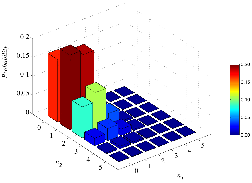
We choose the following parameters for the CME: $\left(\alpha_{1},\alpha_{2},\alpha,\beta_{1},\beta_{2}\right)=(1,0.5,2.5,5,10)$. The choice ensures that the number of any of the two mRNA molecules is limited to $<6$. This results in a small system size in this proof of principle work where the total number of states is $6\times 6=36$. In Fig. 2 panels A and B, we show the numerically observed joint distribution $p_{ss}(n_{1},n_{2})$. The correlated pattern of expression is apparent in panel B; the probability $p_{ss}(n_{2}|n_{1})$ depends on $n_{1}$. The higher the value of $n_{1}$, the higher $n_{2}$ values become more probable as a result of the correlated expression.

In the CME, while there are only 5 rate parameters, there are 145 possible transitions. There are 30 + 30 transitions that correspond to synthesis of mRNA 1 or 2. There are 30 + 30 transitions that correspond to degradation of mRNA 1 or 2 and there are 25 transitions that correspond to simultaneous synthesis of both mRNAs. Each transition has its own rate constant but not all rate constants are independent of each other. For example, the transition $(2,3)\rightarrow(2,2)$ has a rate constant $3\beta_{2}$ and the transition $(2,4)\rightarrow(2,3)$ has a rate constant $4\beta_{2}$. Moreover, many other transition rates are equal to each other, for example, the rates for transitions that increase the first mRNA copy number such as $(1,2)\rightarrow(2,2)$ and $(3,1)\rightarrow(4,1)$ are equal to $\alpha_{1}$ and so on.

We find that Eq. 8 accurately gives the full 145 rate parameters, without the knowledge of the differential rates of synthesis and degradation of the two mRNAs (see supplementary materials for details of the fitting procedure) (see Fig. 3). Taken to larger scale, it implies that using steady state data on cell-to-cell variability in gene expression and a few overall kinetic measurements, we can a full set of chemical master equations and infer regulatory details. This infered model is optimal in the Maximum Caliber sense.

Second, we study the equilibrium dynamics of metastable states of a small peptide comprising 7 alanine amino-acid residues. A metastable state is an ensemble of geometrically and dynamically proximal microstructures that have a significant net population. Classifying protein structures into their metastable states is an active area of research (18, 19, 5, 20).

As a test, we compare to previous extensive MD simulations of this peptide (21), which led to the identification of 32 metastable conformations (20) (see Fig. 4). From that MD simulation, we took the states as defined by Jain and Stock and estimated the relative probability $p_{a}$ of each metastable state $a$ as the fraction of time points in the full trajectory when the peptide was in that state. We also estimated the transition probabilities $k_{ab}$ as the fraction of the events in the trajectory when the peptide was in state $a$ at time $t$ and transitioned into state $b$ at time $t+\delta t$ ($\delta t=1$ ps in a MD simulation of total duration $T=800$ ns).

To predict the transition probabilities $k_{ab}$, we first need to estimate the transition rate matrix ${\bf\Omega}$ using Eq. 9. In order to guess the functional form of the transition rate matrix, we need to identify a dynamical constraint. The accuracy of our predictions depends on how well the dynamical constraint captures the diffusion of the peptide on the free energy landscape. Unfortunately, there is no systematic procedure to guess a ‘good’ constraint variable. This is a common aspect of Maximum-Entropy methods. See (22, 23, 24) for a discussion on the role of constraints in maximum entropy methods.

To guess the dynamical constraint, we make two observations: the transition rate decreases when 1) when the average conformational separation between states is increased, keeping the stationary probabilities and the free energy barrier constant and 2) when the free energy barrier is increased, keeping the average conformational distance and the stationary state probabilities constant. As a first guess, we only model the effect of geometric separation and neglect the free energy barrier. We choose a simple geometric constraint $r_{ab}$: for any two metastable states $a$ and $b$ and microstates $x$ and $y$ such that $x\in a$ and $y\in b$, $r_{ab}=\left(\int_{x\in a,y\in b}||x-y||_{2}dxdy\right)^{\frac{1}{2}}$. $r_{ab}$ is the mean distance between a randomly chosen microstate point $x$ in metastable state $a$ and randomly chosen microstate point $y$ in metastable state $b$. Similarly, $r_{aa}$ is the average distance between any two microstates $x$ and $y$ within a macrostate $a$; it represents the ‘volume’ of macrostate $a$. The distance between any two microstates $x$ and $y$ is defined as the Euclidean distance between their internal coordinate representation (20). The dynamical average $\langle r_{ab}\rangle$ represents the average distance travelled by the microstates of the peptide per unit time.

Using Eq. 9, the numerically estimated stationary probabilities, and the chosen geometric constraint, we arrive at the functional form of the transition rate matrix ${\bf\Omega}$. The transition matrix had two free parameters, $\mu$ the time scale and $\rho$ the Lagrange multiplier associated with $\langle r_{ab}\rangle$. In order to estimate the transition probability matrix ${\bf k}$ from the predicted matrix of transition rates ${\bf\Omega}$, we need the discretization time scale $\delta t$, a third parameter. Since $\mu$ and $\delta t$ can be combined together, we only needed to determine 2 parameters, $\rho$ and $\mu\delta t$. Note that the Maximum Caliber approach guesses the parametric form of the transition probabilities, one can use any suitable numerical technique and experimental information to estimate the parameters. Since we have access to microscopic data, in this proof of principle study, we used the entire transition probability matrix to fit the two free parameters. Using multiple simulated annealing runs to minimize the total error between known and predicted transition probabilities, we found that the best fits were at $\mu\delta t=45\pm 5$ and $\rho=4.8\pm 0.6$. Fig. 5 shows that the rates predicted by the Max Cal approach quite accurately capture the correct values obtained from the full MD simulation, over 5 orders of magnitudes of rates.

For notational simplicity, we derive Eq. 8 for one dynamical constraints $r_{ab}$. Differentiating the Caliber in Eq.  with respect to $k_{ab}$ and setting the derivative to zero,

where $\frac{\beta_{a}}{p_{a}}=e^{m_{a}-1}$, $\lambda_{b}=e^{l_{b}}$, and ${\bf W}_{ab}=e^{-\gamma N_{ab}-\rho r_{ab}}$.

For a given value of $\gamma$ and $\rho$, the Lagrange multipliers $\beta$s and $\lambda$s are determined by self consistently solving Eqs. 3. We have

To further simplify Eqs. 14, let usidentify $\bar{\lambda}$ and $\bar{\beta}$ as the vectors of Lagrange multipliers and define $\mathcal{D}[\bar{x}]_{a}=\frac{p_{a}}{x_{a}}$, a non-linear operator on vectors $\bar{x}$. We have

Now, we write ${\bf W}={\bf I}+\mu\delta t{\bf\Delta}$ where $e^{-\gamma}=\mu\delta t$, ${\bf\Delta}_{ab}=0$ if $(a,b)\notin E$, and ${\bf\Delta}_{ab}=e^{-\rho r_{ab}}$ when $(a,b)\in E$. We have

where

We solve these two equations algebraicly recognizing that $f_{a}$ and $g_{a}$ do not directly depend on $\lambda_{a}$ and $\beta_{a}$. The positive roots are

Given that we’re only interested in transition probabilities $k_{ab}$ up to orders of $\delta t$ and $k_{ab}=\mu\delta t\frac{\beta_{a}}{p_{a}}\lambda_{b}\Delta_{ab}$ already has a $\delta t$ term, we only need to the zeroth order terms for $\bar{\lambda}$ and $\bar{\beta}$ as $\delta t\rightarrow 0$. We solve the algebraic equations 16 simultaneously for $\lambda_{a}$ and $\beta_{a}$ in terms of $f_{a}$, $g_{a}$, $p_{a}$, and $dt$. We then take only the zeroth order terms in $\delta t$ (see supplementary materials for details). We have

Eq. 20 and Eq. 17 can be self-consistently solved for $\bar{\lambda}$ and $\bar{\beta}$ and we can obtain $\bar{f}={\bf\Delta}\bar{\lambda}$ and $\bar{g}={\bf\Delta^{\rm T}}\bar{\beta}$.

As mentioned in the main text, we have assumed for convenience that the dynamical constraints $r_{ab}$ is such that $r_{aa}=0$. Here, we show that when $r_{aa}\neq 0$, the maximum entropy problem is equivalent to constraining a modified constraints $r^{{\dagger}}_{ab}=r_{ab}-\frac{1}{2}\left(r_{aa}+r_{bb}\right)$.

We start with recognizing ${\bf W}={\bf J}+\mu\delta t{\bf\Delta}$ as above where ${\bf J}$ is a diagonal matrix such that ${\bf J}_{aa}=e^{-\rho r_{aa}}$. We have

where $j_{a}={\bf J}_{aa}$ and $\bar{f}={\bf\Delta}\bar{\lambda}~{\rm and}~\bar{g}={\bf\Delta}^{\rm T}\bar{\beta}$. Again solving to zeroth order in $\delta t$, we get

Finally, the transition probability $k_{ab}$ is given by

where $r^{{\dagger}}_{ab}=r_{ab}-\frac{1}{2}\left(r_{aa}+r_{bb}\right)$. Comparing Eq. 23 to Eq. 8, it is clear that the problem of constraining a dynamical constraint $r_{ab}$ such that $r_{aa}$ is non-zero is equivalent to constraining a modified dynamical constraint $r^{{\dagger}}_{ab}=r_{ab}-\frac{1}{2}\left(r_{aa}+r_{bb}\right)$. Note that by definition, $r^{{\dagger}}_{aa}=0$. Thus, for convenience, we assume that this transformation is already performed and $r_{aa}=0$.

From the numerical experiments, we obtain accurate estimate of the stationary state probability distribution $p_{ss}(n_{1},n_{2})$. Let $a\equiv(n_{1},n_{2})$ and $b\equiv(n_{1}^{\dagger},n_{2}^{\dagger})$ be any two states of the system. We know that there is a directed edge from state $a$ to state $b$ iff

1. 1.

   Synthesis or degradation of mRNA 1: $n_{1}=n_{1}^{\dagger}\pm 1$ and $n_{2}=n_{2}$

2. 2.

   Synthesis or degradation of mRNA 2: $n_{1}=n_{1}^{\dagger}$ and $n_{2}=n_{2}^{\dagger}\pm 1$

3. 3.

   Simultaneous synthesis: $n_{1}^{\dagger}=n_{1}+1$ and $n_{2}^{\dagger}=n_{2}+1$

As mentioned in the main text, the ‘experiments’ tell us the total number of degradation and synthesis events per unit time but do not have the ability to distinguish between the two mRNAs. We constrain two quantities, the number of degradation events per unit time and the number of synthesis events per unit time. Accordignly, we set ${\bf\Delta}$ in Eq. 8 as follows

1. 1.

   No edge between nodes $a$ and $b$: ${\bf\Delta}_{ab}=0~{\rm if}~(a,b)\not\in E$

2. 2.

   Synthesis events: ${\bf\Delta}_{ab}=\eta~{\rm if}~n_{1}=n_{1}^{\dagger}~{\rm and}~n_{2}+1=n_{2}^{\dagger}~{\rm or}~n_{1}+1=n_{1}^{\dagger}~{\rm and}~n_{2}=n_{2}^{\dagger}~{\rm or}~~n_{1}+1=n_{1}^{\dagger}~{\rm and}~n_{2}+1=n_{2}^{\dagger}$

3. 3.

   Degradation of mRNA 1: ${\bf\Delta}_{ab}=n_{1}\zeta~{\rm if}~n_{1}=n_{1}^{\dagger}+1~{\rm and}~n_{2}=n_{2}^{\dagger}$

4. 4.

   Degradation of mRNA2: ${\bf\Delta}_{ab}=n_{2}\zeta~{\rm if}~n_{1}=n_{1}^{\dagger}~{\rm and}~n_{2}=n_{2}^{\dagger}+1$

Here, $\eta\geq 0$ and $\zeta\geq 0$ are exponentials of Lagrange multipliers similar to those used in the main text. The Lagrange rate constant $\mu$ in Eq. 8 is assumed to be absorbed in the Lagrange multipliers. The next step is to determine $\bar{f}$, $\bar{g}$, $\bar{\lambda}$, and $\bar{\beta}$ using numerically estimated $p_{ss}(n_{1},n_{2})$ and ${\bf\Delta}$. In order to determine the transition rate matrix ${\bf\Omega}$ for any value of $\eta$ and $\zeta$, we solve Eq. 17 and Eq. 20 self consistently.

Given that we have access to all rate constants in this proof of principles work, we minimize the error between the known rate constants of Eq.  and those predicted by Eq. 8 by varying $\eta$ and $\zeta$ using a simulated annealing protocol. We find that $\eta\approx 0.4$ and $\zeta\approx 26.5$ resulted in the best agreement between the known and the predicted rate constants. Multiple simulated annealing runs predicted rates that were identical to the ones shown in the main text. Note that although we used the entire transition matrix to learn the Lagrange multipliers, it is equally possible to learn them from global dynamical constraints.

References

- (1) Schneidman, E., M. J. Berry, R. Segev, and W. Bialek, 2006. Weak pairwise correlations imply strongly correlated network states in a neural population. Nature 440:1007–1012.
- (2) Shekhar, K., C. F. Ruberman, A. L. Ferguson, J. P. Barton, M. Kardar, and A. K. Chakraborty, 2013. Spin models inferred from patient-derived viral sequence data faithfully describe HIV fitness landscapes. Physical review E 88:062705.
- (3) Han, Y., Y. Shokef, A. M. Alsayed, P. Yunker, T. C. Lubensky, and A. G. Yodh, 2008. Geometric frustration in buckled colloidal monolayers. Nature 456:898–903.
- (4) Orth, J. D., I. Thiele, and B. Ø. Palsson, 2010. What is flux balance analysis? Nature biotechnology 28:245–248.
- (5) Chodera, J. D., and F. Noé, 2014. Markov state models of biomolecular conformational dynamics. Current opinion in structural biology 25:135–144.
- (6) Pressé, S., K. Ghosh, J. Lee, and K. A. Dill, 2013. The principles of Maximum Entropy and Maximum Caliber in statistical physics. Rev. Mod. Phys. 85:1115–1141.
- (7) Peterson, J., P. D. Dixit, and K. A. Dill, 2013. A maximum entropy framework for nonexponential distributions. Proc. Natl. Acad. Sci. 110:20380–20385.
- (8) Filyukov, A., and V. Y. Karpov, 1967. Method of the most probable path of evolution in the theory of stationary irreversible processes. J. Engg. Phys. Thermophys. 13:416–419.
- (9) Dixit, P. D., and K. A. Dill, 2014. Inferring microscopic kinetic rates from stationary state distributions. Journal of chemical theory and computation 10:3002–3005.
- (10) Cover, T. M., and J. A. Thomas, 2012. Elements of information theory. John Wiley & Sons.
- (11) Stock, G., K. Ghosh, and K. A. Dill, 2008. Maximum Caliber: A variational approach applied to two-state dynamics. J. Chem. Phys. 128:194102.
- (12) Glauber, R. J., 1963. Time-dependent statistics of the Ising model. Journal of mathematical physics 4:294.
- (13) Mariz, A., H. Herrmann, and L. de Arcangelis, 1990. Comparative study of damage spreading in the Ising model using heat-bath, glauber, and metropolis dynamics. Journal of Statistical Physics 59:1043–1050.
- (14) Leffler, J. E., and E. Grunwald, 2013. Rates and equilibria of organic reactions: as treated by statistical, thermodynamic and extrathermodynamic methods. Courier Corporation.
- (15) Michaelides, A., Z.-P. Liu, C. Zhang, A. Alavi, D. A. King, and P. Hu, 2003. Identification of general linear relationships between activation energies and enthalpy changes for dissociation reactions at surfaces. Journal of the American Chemical Society 125:3704–3705.
- (16) Marcus, R. A., 1968. Theoretical relations among rate constants, barriers, and Brønsted slopes of chemical reactions. The Journal of Physical Chemistry 72:891–899.
- (17) Matouschek, A., and A. R. Fersht, 1993. Application of physical organic chemistry to engineered mutants of proteins: Hammond postulate behavior in the transition state of protein folding. Proceedings of the National Academy of Sciences 90:7814–7818.
- (18) Lane, T. J., G. R. Bowman, K. Beauchamp, V. A. Voelz, and V. S. Pande, 2011. Markov state model reveals folding and functional dynamics in ultra-long MD trajectories. Journal of the American Chemical Society 133:18413–18419.
- (19) Prinz, J.-H., H. Wu, M. Sarich, B. Keller, M. Senne, M. Held, J. D. Chodera, C. Schütte, and F. Noé, 2011. Markov models of molecular kinetics: Generation and validation. The Journal of chemical physics 134:174105.
- (20) Jain, A., and G. Stock, 2012. Identifying metastable states of folding proteins. Journal of Chemical Theory and Computation 8:3810–3819.
- (21) Altis, A., M. Otten, P. H. Nguyen, R. Hegger, and G. Stock, 2008. Construction of the free energy landscape of biomolecules via dihedral angle principal component analysis. The Journal of chemical physics 128:245102.
- (22) Caticha, A., and R. Preuss, 2004. Maximum entropy and Bayesian data analysis: Entropic prior distributions. Phys. Rev. E 70:046127.
- (23) Caticha, A., 2012. Entropic Inference: some pitfalls and paradoxes we can avoid. arXiv preprint arXiv:1212.6967 .
- (24) Dixit, P. D., 2013. Quantifying Extrinsic Noise in Gene Expression Using the Maximum Entropy Framework. Biophys. J. 104:2743–2750.
- (25) Mora, T., A. M. Walczak, W. Bialek, and C. G. Callan, 2010. Maximum entropy models for antibody diversity. Proceedings of the National Academy of Sciences 107:5405–5410.
- (26) Paulsson, J., 2004. Summing up the noise in gene networks. Nature 427:415–418.
- (27) Baldi, P., P. Frasconi, and P. Smyth, 2003. Modeling the Internet and the Web. Probabilistic methods and algorithms .
V Supplementary materials
V.1 Deriving the maximum Caliber transition rates