跳到论文正文
W Papers独立论文阅读器 arXiv:1504.01204 论文正文 计算阅读时间 · 0%
引用这篇论文根据当前论文元数据生成,正式投稿前建议核对。


License: arXiv.org perpetual non-exclusive license
arXiv:1504.01204v2 [hep-ph] 26 Mar 2016

Radiative Seesaw in Minimal 3-3-1 Model

Preprint: KIAS-P15017
Hiroshi Okada Email: hokada@kias.re.kr Affiliation: School of Physics, KIAS, Seoul 130-722, Korea    Nobuchika Okada Email: okadan@ua.edu Affiliation: Department of Physics and Astronomy, University of Alabama, Tuscaloosa, AL35487, USA    Yuta Orikasa Email: orikasa@kias.re.kr Affiliation: School of Physics, KIAS, Seoul 130-722, Korea Affiliation: Department of Physics and Astronomy, Seoul National University, Seoul 151-742, Korea
August 24, 2026
Abstract

We study the neutrino sector in a minimal S​U​(3)L×U​(1)XSU(3)_{L}\times U(1)_{X} model, in which its mass is generated at one-loop level with the charged lepton mass, and hence there exists a strong correlation between the charged-lepton mass and the neutrino mass. We identify the parameter region of this model to satisfy the current neutrino oscillation data as well as the constraints on lepton flavor violating processes. We also discuss a possibility to explain the muon anomalous magnetic moment.

Keywords: 
3-3-1, radiative neutrino masses, lepton flavor violations

I Introduction

The flavor problem can be one of the biggest challenging issues to be resolved, since the standard model (SM) does not have any theoretical sources (especially) why the number of family for each fermion sector (quarks and leptons) is three. One of the reasonable interpretations is to extend the gauge sector S​U​(2)L×U​(1)YSU(2)_{L}\times U(1)_{Y} to S​U​(3)L×U​(1)XSU(3)_{L}\times U(1)_{X}, so called 3-3-1 model, in which the origin of three family is coming from the number of S​U​(3)SU(3) color of quarks (that has three) due to the gauge anomaly cancellation [1, 2]. Because of larger gauge group comparing to the SM one, there are several variations of models extending the Higgs sector  [3, 4, 5, 6, 7] and revisited models to reanalyze with current experimental data [8, 9, 10, 11, 12, 13, 14, 15, 16, 17, 18, 19, 20, 21, 22, 23, 24, 25, 26, 27, 28, 29].

On the other hand, explaining the current neutrino oscillation data and dark matter (DM) candidate might be done by physics beyond SM. It is known that in recent radiative seesaw models they can be only explained simultaneously but also correlated each other. It means that neutrinos do not directly interact with the SM Higgs field but with a DM candidate. As a result, minuscule neutrino masses can be naturally realized. This is because a vast literature has recently arisen along thought of this subject [30, 31, 32, 33, 34, 35, 36, 37, 38, 39, 40, 41].

In this paper, we combine the 3-3-1 model and radiative seesaw model based on a minimal model in Ref. [5], in which we do not impose any additional discrete symmetry. Then we can generate the neutrino mass at one-loop level. Moreover since our model has a strong correlation between the charged lepton sector and the neutrino sector due to the same origin of these masses, it may be worth analyzing the neutrino oscillation data as well as lepton flavor violating processes and so on.

This paper is organized as follows. In Sec. II, we show our model including Higgs potential. In Sec. III, we analyze lepton sector and show how to correlate the charged-lepton masses and neutrino masses. Then we also show to compute lepton flavor violating processes and muon anomalous magnetic moment. In Sec. IV, we perform parameter scan to identify allowed parameter regions. We conclude in Sec. V.

Lepton Fields Scalar Fields
 LL=(νL,eL,eRc)L_{L}=(\nu_{L},e_{L},e^{c}_{R})  SS  η\eta  ρ\rho  χ\chi
S​U​(3)LSU(3)_{L} 𝟑\bm{3} 𝟔\bm{6} 𝟑\bm{3} 𝟑\bm{3} 𝟑\bm{3}
U​(1)XU(1)_{X} 00 00 00 11 −1-1
Table 1: Contents of lepton and scalar fields and their charge assignment under S​U​(3)L×U​(1)XSU(3)_{L}\times U(1)_{X}, where the index of the generation are abbreviated.

II Model setup

We discuss a possibility of a one-loop induced radiative seesaw model in the context of 3-3-1 model in [5]. The particle contents are shown in Tab. 1. We introduce a gauge triplet fermion LL=(νL,eL,eRc)L_{L}=(\nu_{L},e_{L},e^{c}_{R}) with U​(1)XU(1)_{X}=0. For new bosons, we introduce S​U​(3)LSU(3)_{L} sextet scalars SS with U​(1)XU(1)_{X}=0, S​U​(3)LSU(3)_{L} triplet scalars (η,ρ,χ\eta,\rho,\chi) with U​(1)X=(0,1,−1)U(1)_{X}=(0,1,-1), respectively. The renormalizable Lagrangian for Lepton Yukawa sector, and the scalar potential under these assignments are given by

ℒY\displaystyle\mathcal{L}_{Y} =yℓ1​∑i,j,k=1−3L¯L​i​(LL)jc​ηk∗​ϵi​j​k+yℓ2​Tr​[L¯L​S​(LL)c]+h.c.\displaystyle=y_{\ell_{1}}\sum_{i,j,k=1-3}\bar{L}_{Li}(L_{L})^{c}_{j}\eta^{*}_{k}\epsilon^{ijk}+y_{\ell_{2}}{\rm Tr}[\bar{L}_{L}S(L_{L})^{c}]+\rm{h.c.} (II.1)
𝒱\displaystyle\mathcal{V} =mη2​|η|2+mρ2​|ρ|2+mχ2​|χ|2+mS2​Tr​[|S|2]\displaystyle=m_{\eta}^{2}|\eta|^{2}+m_{\rho}^{2}|\rho|^{2}+m_{\chi}^{2}|\chi|^{2}+m_{S}^{2}{\rm Tr}[|S|^{2}]
+λ1​|η|4+λ2​|ρ|4+λ3​|χ|4+λ4​[Tr⁡[|S|]]4+λ5​Tr​[|S|4]+λ6​|η|2​|ρ|2+λ7​|η|2​|χ|2+λ8​|χ|2​|ρ|2\displaystyle+\lambda_{1}|\eta|^{4}+\lambda_{2}|\rho|^{4}+\lambda_{3}|\chi|^{4}+\lambda_{4}[{\rm Tr}[|S|]]^{4}+\lambda_{5}{\rm Tr}[|S|^{4}]+\lambda_{6}|\eta|^{2}|\rho|^{2}+\lambda_{7}|\eta|^{2}|\chi|^{2}+\lambda_{8}|\chi|^{2}|\rho|^{2}
+λ9​|η|2​Tr​[|S|2]+λ10​|ρ|2​Tr​[|S|2]+λ11​|χ|2​Tr​[|S|2]+λ12​|ρ†​η|2+λ13​|χ†​η|2+λ14​|ρ†​χ|2\displaystyle+\lambda_{9}|\eta|^{2}{\rm Tr}[|S|^{2}]+\lambda_{10}|\rho|^{2}{\rm Tr}[|S|^{2}]+\lambda_{11}|\chi|^{2}{\rm Tr}[|S|^{2}]+\lambda_{12}|\rho^{\dagger}\eta|^{2}+\lambda_{13}|\chi^{\dagger}\eta|^{2}+\lambda_{14}|\rho^{\dagger}\chi|^{2}
+(m1∑i,j,k=1−3ϵi​j​kηiρjχk+h.c.)+(m2ρTS†χ+h.c.)+(m3ηTSη+h.c.)\displaystyle+(m_{1}\sum_{i,j,k=1-3}\epsilon^{ijk}\eta_{i}\rho_{j}\chi_{k}+{\rm h.c.})+(m_{2}\rho^{T}S^{\dagger}\chi+{\rm h.c.})+(m_{3}\eta^{T}S\eta+{\rm h.c.})
+(m4∑i,j,k1−3∑l,m,n1−3ϵi​j​kϵl​m​nSi​lSj​mSk​n+h.c.)+(f5(η†ρ)(η†χ)+h.c.)+(f6∑i,j,k1−3ϵi​j​kSl​iρjχkηl∗+h.c.)\displaystyle+(m_{4}\sum_{i,j,k}^{1-3}\sum_{l,m,n}^{1-3}\epsilon^{ijk}\epsilon^{lmn}S_{il}S_{jm}S_{kn}+{\rm h.c.})+(f_{5}(\eta^{\dagger}\rho)(\eta^{\dagger}\chi)+{\rm h.c.})+(f_{6}\sum_{i,j,k}^{1-3}\epsilon^{ijk}S_{li}\rho_{j}\chi_{k}\eta^{*}_{l}+{\rm h.c.})
+f7Tr[S†Sη∗ηT]+f8Tr[S†Sρ∗ρT]+f9Tr[S†Sχ∗χT]+(f10∑i,j,k1−3∑l,m,n1−3ϵi​j​kϵl​m​nSi​lSj​mηkηn+h.c.),\displaystyle+f_{7}{\rm Tr}[S^{\dagger}S\eta^{*}\eta^{T}]+f_{8}{\rm Tr}[S^{\dagger}S\rho^{*}\rho^{T}]+f_{9}{\rm Tr}[S^{\dagger}S\chi^{*}\chi^{T}]+(f_{10}\sum_{i,j,k}^{1-3}\sum_{l,m,n}^{1-3}\epsilon^{ijk}\epsilon^{lmn}S_{il}S_{jm}\eta_{k}\eta_{n}+{\rm h.c.}), (II.2)

where yℓ1y_{\ell_{1}} is an anti-symmetric 3 by 3 matrix and yℓ2y_{\ell_{2}} is a symmetric one. Here the scalar fields can be parameterized as

S\displaystyle S =[σ10h2−h1+h2−H1−⁣−σ20h1+σ20H2+⁣+],η=[η0η1−η2+],ρ=[ρ+ρ0η+⁣+],χ=[χ−χ−⁣−χ0],σ10=σ1​R+i​σ1​I2,\displaystyle=\left[\begin{array}[]{ccc}\sigma_{1}^{0}&h_{2}^{-}&h_{1}^{+}\\ h_{2}^{-}&H_{1}^{--}&\sigma_{2}^{0}\\ h_{1}^{+}&\sigma_{2}^{0}&H_{2}^{++}\end{array}\right],\quad\eta=\left[\begin{array}[]{c}\eta^{0}\\ \eta^{-}_{1}\\ \eta^{+}_{2}\end{array}\right],\quad\rho=\left[\begin{array}[]{c}\rho^{+}\\ \rho^{0}\\ \eta^{++}\end{array}\right],\quad\chi=\left[\begin{array}[]{c}\chi^{-}\\ \chi^{--}\\ \chi^{0}\end{array}\right],\sigma_{1}^{0}=\frac{\sigma_{1R}+i\sigma_{1I}}{\sqrt{2}},\quad
σ20\displaystyle\sigma_{2}^{0} =vσ+σ2​R+i​σ2​I2,η0=vη+ηR+i​ηI2,ρ0=vρ+ρR+i​ρI2,χ0=vχ+χR+i​χI2.\displaystyle=\frac{v_{\sigma}+\sigma_{2R}+i\sigma_{2I}}{\sqrt{2}},\quad\eta^{0}=\frac{v_{\eta}+\eta_{R}+i\eta_{I}}{\sqrt{2}},\quad\rho^{0}=\frac{v_{\rho}+\rho_{R}+i\rho_{I}}{\sqrt{2}},\quad\chi^{0}=\frac{v_{\chi}+\chi_{R}+i\chi_{I}}{\sqrt{2}}. (II.15)

Here v=vσ2+vη2+vρ2=246v=\sqrt{v_{\sigma}^{2}+v_{\eta}^{2}+v_{\rho}^{2}}=246 GeV is the vacuum expectation value (vev), and we have assumed that the vev of σ10\sigma_{1}^{0} is zero, which is unlike the original model discussed in [5]. The scale of vχv_{\chi}, which breaks S​U​(3)LSU(3)_{L} symmetry, is assumed to be of 𝒪{\cal O}(1) TeV, while the other three vevs (vσ,vρ,vηv_{\sigma},v_{\rho},v_{\eta}) are assumed to be 𝒪{\cal O}(1-100) GeV.

III Lepton sector

III.1 Charged lepton sector

The charged lepton masses can be generated by the terms yℓ1​∑i,j,k=1−3L¯L​i​(LL)jc​ηk∗​ϵi​j​ky_{\ell_{1}}\sum_{i,j,k=1-3}\bar{L}_{Li}(L_{L})^{c}_{j}\eta^{*}_{k}\epsilon^{ijk} and yℓ2​Tr​[L¯L​S​(LL)c]y_{\ell_{2}}{\rm Tr}[\bar{L}_{L}S(L_{L})^{c}] after the electroweak symmetry breaking, as can be seen in Eq. (II.1). The resulting mass matrix can be written and diagonalized by

(e¯L)a​(mℓ)a​b​(eR)b≡(e¯L)a​[(yℓ1)​vη2+(yℓ2)​vσ2]a​b​(eR)b=(e¯L)a​(Ve​L†)a​i​(mℓd​i​a​g)i​(Ve​R)i​b​(eR)b,\displaystyle(\bar{e}_{L})_{a}(m_{\ell})_{ab}(e_{R})_{b}\equiv(\bar{e}_{L})_{a}\left[\frac{(y_{\ell_{1}})v_{\eta}}{\sqrt{2}}+\frac{(y_{\ell_{2}})v_{\sigma}}{\sqrt{2}}\right]_{ab}(e_{R})_{b}=(\bar{e}_{L})_{a}(V^{\dagger}_{eL})_{ai}(m^{diag}_{\ell})_{i}(V_{eR})_{ib}(e_{R})_{b}, (III.1)
∑k=13[(yℓ1)​vη2+(yℓ2)​vσ2]a​k​[(yℓ1)​vη2+(yℓ2)​vσ2]b​k∗=(Ve​L†)a​i​|mℓd​i​a​g|i2​(Ve​L)i​b,\displaystyle\sum_{k=1}^{3}\left[\frac{(y_{\ell_{1}})v_{\eta}}{\sqrt{2}}+\frac{(y_{\ell_{2}})v_{\sigma}}{\sqrt{2}}\right]_{ak}\left[\frac{(y_{\ell_{1}})v_{\eta}}{\sqrt{2}}+\frac{(y_{\ell_{2}})v_{\sigma}}{\sqrt{2}}\right]^{*}_{bk}=(V^{\dagger}_{eL})_{ai}|m^{diag}_{\ell}|^{2}_{i}(V_{eL})_{ib}, (III.2)

where yℓ1y_{\ell_{1}} is the ant-symmetric matrix and yℓ2y_{\ell_{2}} is the symmetric matrix. |mℓd​i​a​g|=(|me|,|mμ|,|mτ|)=(0.5​MeV,105.6​MeV,1777​MeV)|m^{diag}_{\ell}|=(|m_{e}|,|m_{\mu}|,|m_{\tau}|)=(0.5\ {\rm MeV},105.6\ {\rm MeV},1777\ {\rm MeV}). Each of Ve​LV_{eL} and Ve​RV_{eR} is the unitary matrix to diagonalize the charged leptons. From Eq. (III.1) and the properties of anti-symmetric yℓ1y_{\ell_{1}} and of symmetric yℓ2y_{\ell_{2}}, the charged lepton Yukawa couplings yℓ1​(2)y_{\ell_{1(2)}} can explicitly be rewritten in terms of the charged lepton mass matrix as

(yℓ1)a​b=(mℓ)a​b+(mℓ)a​bT2​vη,(yℓ2)a​b=(mℓ)a​b−(mℓ)a​bT2​vσ.\displaystyle(y_{\ell_{1}})_{ab}=\frac{(m_{\ell})_{ab}+(m_{\ell})_{ab}^{T}}{\sqrt{2}v_{\eta}},\quad(y_{\ell_{2}})_{ab}=\frac{(m_{\ell})_{ab}-(m_{\ell})_{ab}^{T}}{\sqrt{2}v_{\sigma}}. (III.3)

Therefore, these Yukawa couplings can be taken as the output parameters, once the charged lepton masses and their mixings are fixed as inputs in the following numerical analysis.

III.2 Neutrino sector
Refer to caption
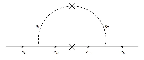
Figure 1: An example of one-loop diagrams contributing to neutrino mass.

Through the following Yukawa interactions,

ℒ\displaystyle{\cal L} ⊃\displaystyle\supset yℓ1​(ν¯L​eLc−e¯L​νLc)​η2−+yℓ1​(−ν¯L​eR+e¯Rc​νLc)​η1+\displaystyle y_{\ell_{1}}(\bar{\nu}_{L}e^{c}_{L}-\bar{e}_{L}\nu^{c}_{L})\eta^{-}_{2}+y_{\ell_{1}}(-\bar{\nu}_{L}e_{R}+\bar{e}^{c}_{R}\nu^{c}_{L})\eta^{+}_{1} (III.4)
+\displaystyle+ yℓ2​(ν¯L​eLc+e¯L​νLc)​h2−+yℓ2​(ν¯L​eR+e¯Rc​νLc)​h1+,\displaystyle y_{\ell_{2}}(\bar{\nu}_{L}e^{c}_{L}+\bar{e}_{L}\nu^{c}_{L})h^{-}_{2}+y_{\ell_{2}}(\bar{\nu}_{L}e_{R}+\bar{e}^{c}_{R}\nu^{c}_{L})h^{+}_{1},

the active neutrino mass matrix mνm_{\nu} is induced at one-loop level (see Fig. 1 for an example diagram), which is given by

−(ℳνth)a​b\displaystyle-({\cal M}_{\nu}^{\rm th})_{ab} ≈[yℓ1​(mℓ†+mℓ∗)​yℓ1T]a​b(4​π)2​[δ​mη1​η2+2mη1+2−mη2+2]​ln⁡[mη1+2mη2+2]\displaystyle\approx\frac{\left[y_{\ell_{1}}\left(m^{\dagger}_{\ell}+m^{*}_{\ell}\right)y^{T}_{\ell_{1}}\right]_{ab}}{(4\pi)^{2}}\left[\frac{\delta m^{+2}_{\eta_{1}\eta_{2}}}{m_{\eta^{+}_{1}}^{2}-m_{\eta^{+}_{2}}^{2}}\right]{\ln\left[\frac{m_{\eta^{+}_{1}}^{2}}{m_{\eta^{+}_{2}}^{2}}\right]}
−[yℓ2​(mℓ†+mℓ∗)​yℓ2T]a​b(4​π)2​[δ​mh1​η2+2mh1+2−mh2+2]​ln⁡[mh1+2mh2+2]\displaystyle-\frac{\left[y_{\ell_{2}}\left(m^{\dagger}_{\ell}+m^{*}_{\ell}\right)y^{T}_{\ell_{2}}\right]_{ab}}{(4\pi)^{2}}\left[\frac{\delta m^{+2}_{h_{1}\eta_{2}}}{m_{h^{+}_{1}}^{2}-m_{h^{+}_{2}}^{2}}\right]{\ln\left[\frac{m_{h^{+}_{1}}^{2}}{m_{h^{+}_{2}}^{2}}\right]}
−(yℓ1​mℓ∗​yℓ2T+yℓ2​mℓ†​yℓ1T)a​b2​(4​π)2​[δ​mη2​h1+2mη2+2−mh1+2]​ln⁡[mη2+2mh1+2]\displaystyle-\frac{\left(y_{\ell_{1}}m^{*}_{\ell}y^{T}_{\ell_{2}}+y_{\ell_{2}}m^{{\dagger}}_{\ell}y^{T}_{\ell_{1}}\right)_{ab}}{2(4\pi)^{2}}\left[\frac{\delta m^{+2}_{\eta_{2}h_{1}}}{m_{\eta^{+}_{2}}^{2}-m_{h^{+}_{1}}^{2}}\right]{\ln\left[\frac{m_{\eta^{+}_{2}}^{2}}{m_{h^{+}_{1}}^{2}}\right]}
−(yℓ2​mℓ∗​yℓ1T+yℓ1​mℓ†​yℓ2T)a​b2​(4​π)2​[δ​mη1​h2+2mη1+2−mh2+2]​ln⁡[mη1+2mh2+2].\displaystyle-\frac{\left(y_{\ell_{2}}m^{*}_{\ell}y^{T}_{\ell_{1}}+y_{\ell_{1}}m^{{\dagger}}_{\ell}y^{T}_{\ell_{2}}\right)_{ab}}{2(4\pi)^{2}}\left[\frac{\delta m^{+2}_{\eta_{1}h_{2}}}{m_{\eta^{+}_{1}}^{2}-m_{h^{+}_{2}}^{2}}\right]{\ln\left[\frac{m_{\eta^{+}_{1}}^{2}}{m_{h^{+}_{2}}^{2}}\right]}. (III.5)

Note here that the mass insertion approximation has been used, that is, (M+)2=(M+)diag2+(M+)off−diag2(M_{+})^{2}=(M_{+})^{2}_{\rm diag}+(M_{+})^{2}_{\rm off-diag} with (M+)diag2≫(M+)off−diag2≡δ​mfi​fj′+2,(fi,fj′=ηi,hj)(M_{+})^{2}_{\rm diag}\gg(M_{+})^{2}_{\rm off-diag}\equiv\delta m^{+2}_{f_{i}f^{\prime}_{j}},\ (f_{i},f^{\prime}_{j}=\eta_{i},h_{j}), where M+M_{+} is the singly charged boson mass matrix, and

mh1+2≈f9​vχ2,mh2+2≈m2​vχ​vρvσ,mη1+2≈m1​vχ​vρvη,mη2+2≈λ13​vχ2,\displaystyle m^{2}_{h_{1}^{+}}\approx f_{9}v^{2}_{\chi},\quad m^{2}_{h_{2}^{+}}\approx\frac{m_{2}v_{\chi}v_{\rho}}{v_{\sigma}},\quad m^{2}_{\eta_{1}^{+}}\approx\frac{m_{1}v_{\chi}v_{\rho}}{v_{\eta}},\quad m^{2}_{\eta_{2}^{+}}\approx{\lambda_{13}v_{\chi}^{2}},
δ​mη1​η2+2=2​m3​vη+(f5​vρ​vχ)/2,δ​mh1​h2+2=3​2​m4​vσ,\displaystyle\delta m^{+2}_{\eta_{1}\eta_{2}}=\sqrt{2}m_{3}v_{\eta}+(f_{5}v_{\rho}v_{\chi})/2,\;\delta m^{+2}_{h_{1}h_{2}}=3\sqrt{2}m_{4}v_{\sigma},
δ​mη1​h1+2=(4​f10+f7)​vσ​vη/(2​2),δ​mη2​h1+2=m3​vη+(f6​vρ​vχ)/(2​2),\displaystyle\delta m^{+2}_{\eta_{1}h_{1}}=(4f_{10}+f_{7})v_{\sigma}v_{\eta}/(2\sqrt{2}),\;\delta m^{+2}_{\eta_{2}h_{1}}=m_{3}v_{\eta}+(f_{6}v_{\rho}v_{\chi})/(2\sqrt{2}),
δ​mη1​h2+2=m3​vη+(f6​vρ​vχ)/(2​2),δ​mη2​h2+2=(4​f10+f7)​vσ​vη/(2​2).\displaystyle\delta m^{+2}_{\eta_{1}h_{2}}=m_{3}v_{\eta}+(f_{6}v_{\rho}v_{\chi})/(2\sqrt{2}),\;\delta m^{+2}_{\eta_{2}h_{2}}=(4f_{10}+f_{7})v_{\sigma}v_{\eta}/(2\sqrt{2}). (III.6)

It suggests m1,m2≫m3,m4m_{1},m_{2}\gg m_{3},m_{4} and f9,λ13≫f5,f6,f7,f10f_{9},\lambda_{13}\gg f_{5},f_{6},f_{7},f_{10}.

Neutrino mass matrix can be diagonalized by a unitary matrix UνU_{\nu} as mν=Uν​mνd​i​a​g​UνTm_{\nu}=U_{\nu}m_{\nu}^{diag}U^{T}_{\nu}, and hence the MNS matrix UMNSU_{\rm MNS} is defined as

UMNS=Ve​L†​Uν.\displaystyle U_{\rm MNS}=V^{\dagger}_{eL}U_{\nu}. (III.7)

III.3 Lepton Flavor Violations

Here we discuss the lepton flavor violating processes in our model, which can be induced through the mixings among singly charged bosons in Eq. (III.4). The branching ratio of the lepton flavor violating decays are given by

BR⁡(ℓi→ℓj​γ)\displaystyle{\rm BR}(\ell_{i}\to\ell_{j}\gamma) =12​π2mi2​GF2​[|AL​j​i|2+|AR​j​i|2],\displaystyle=\frac{12\pi^{2}}{m_{i}^{2}{\rm G_{F}}^{2}}\left[|A_{Lji}|^{2}+|A_{Rji}|^{2}\right], (III.8)

where

AL​j​i\displaystyle A_{Lji} =mj​[GL(i​i)​(η2,h2)+GL(i​i​i+v)​(η2,h2)]j​i+mi​[GL(i)​(η1,h1)+GL(i​v+v​i)​(η1,h1)]j​i,\displaystyle=m_{j}\left[G^{(ii)}_{L}(\eta_{2},h_{2})+G^{(iii+v)}_{L}(\eta_{2},h_{2})\right]_{ji}+m_{i}\left[G^{(i)}_{L}(\eta_{1},h_{1})+G^{(iv+vi)}_{L}(\eta_{1},h_{1})\right]_{ji}, (III.9)
AR​j​i\displaystyle A_{Rji} =mj​[GR(i)​(η1,h1)+GR(i​v+v​i)​(η1,h1)]j​i+mi​[GR(i​i)​(η2,h2)+GR(i​i​i+v)​(η2,h2)]j​i,\displaystyle=m_{j}\left[G^{(i)}_{R}(\eta_{1},h_{1})+G^{(iv+vi)}_{R}(\eta_{1},h_{1})\right]_{ji}+m_{i}\left[G^{(ii)}_{R}(\eta_{2},h_{2})+G^{(iii+v)}_{R}(\eta_{2},h_{2})\right]_{ji}, (III.10)
GL⁡(R)(i)​(η1,h1)≈δ​mη1​h1+2​[(yℓ2†​yℓ1)′+(yℓ1†​yℓ2)′]12​(4​π)2​mη12​mh12,\displaystyle G^{(i)}_{L(R)}(\eta_{1},h_{1})\approx\frac{\delta m^{+2}_{\eta_{1}h_{1}}[(y_{\ell_{2}}^{\dagger}y_{\ell_{1}})^{\prime}+(y_{\ell_{1}}^{\dagger}y_{\ell_{2}})^{\prime}]}{12(4\pi)^{2}m_{\eta_{1}}^{2}m_{h_{1}}^{2}}, (III.11)
GL⁡(R)(i​i)​(η2,h2)≈δ​mη2​h2+2​[(yℓ1​yℓ2†)′+(yℓ2​yℓ1†)′]12​(4​π)2​mη22​mh22,\displaystyle G^{(ii)}_{L(R)}(\eta_{2},h_{2})\approx\frac{\delta m^{+2}_{\eta_{2}h_{2}}[(y_{\ell_{1}}y_{\ell_{2}}^{\dagger})^{\prime}+(y_{\ell_{2}}y_{\ell_{1}}^{\dagger})^{\prime}]}{12(4\pi)^{2}m_{\eta_{2}}^{2}m_{h_{2}}^{2}}, (III.12)
GL⁡(R)(i​i​i+v)​(η1,h1)≈GL⁡(R)(i​v+v​i)​(η2,h2)≈112​(4​π)2​[(yℓ1​yℓ1†)′mη22+(yℓ2​yℓ2†)′mh22],\displaystyle G^{(iii+v)}_{L(R)}(\eta_{1},h_{1})\approx G^{(iv+vi)}_{L(R)}(\eta_{2},h_{2})\approx\frac{1}{12(4\pi)^{2}}\left[\frac{(y_{\ell_{1}}y_{\ell_{1}}^{\dagger})^{\prime}}{m_{\eta_{2}}^{2}}+\frac{(y_{\ell_{2}}y_{\ell_{2}}^{\dagger})^{\prime}}{m_{h_{2}}^{2}}\right], (III.13)

with (yℓa†​yℓb)′≡Ve​R​yℓa†​yℓb​Ve​R†(y_{\ell_{a}}^{\dagger}y_{\ell_{b}})^{\prime}\equiv V_{eR}y_{\ell_{a}}^{\dagger}y_{\ell_{b}}V_{eR}^{\dagger}, and (yℓa​yℓb†)′≡Ve​L​yℓa​yℓb†​Ve​L†(y_{\ell_{a}}y_{\ell_{b}}^{\dagger})^{\prime}\equiv V_{eL}y_{\ell_{a}}y_{\ell_{b}}^{\dagger}V_{eL}^{\dagger}, with (a,b)=1,2(a,b)=1,2. The upper indices of GG, respectively, represent a difference among the singly charged bosons exchanging processes. Therefore, (i)(i) is the η1+\eta_{1}^{+} and h1+h_{1}^{+} mixing process, (i​i)(ii) is the η2+\eta_{2}^{+} and h2+h_{2}^{+} mixing one, (i​i​i)(iii) is the η1+\eta_{1}^{+} no mixing one, (i​v)(iv) is the η2+\eta_{2}^{+} no mixing one, (v)(v) is the h1+h_{1}^{+} no mixing one, and (v​i)(vi) is the h2+h_{2}^{+} no mixing one.

There are box types of LFV precesses ℓa−→ℓb−​ℓc+​ℓd−\ell_{a}^{-}\to\ell_{b}^{-}\ell_{c}^{+}\ell_{d}^{-} through yℓ1,2y_{\ell_{1,2}} in general, however we expect such processes are negligibly small when our mass insertion approximation is reliable. The penguin types of these LFV processes are also negligible, comparing to the ℓi→ℓj​γ\ell_{i}\to\ell_{j}\gamma one-loop induced processes [42].

III.4 Muon Anomalous Magnetic Moment

The muon anomalous magnetic moment, so-called the muon g−2g-2, has been measured at Brookhaven National Laboratory. The current average of the experimental results is given by [43]

aμexp=11659208.0​(6.3)×10−10.\displaystyle a^{\rm exp}_{\mu}=11659208.0(6.3)\times 10^{-10}. (III.14)

It has been known that there is a discrepancy from the SM prediction by 3.2​σ3.2\sigma [44] to 4.1​σ4.1\sigma [45]:

Δ​aμ=aμexp−aμSM=(29.0±9.0​to​ 33.5±8.2)×10−10.\displaystyle\Delta a_{\mu}=a^{\rm exp}_{\mu}-a^{\rm SM}_{\mu}=(29.0\pm 9.0\ {\rm to}\ 33.5\pm 8.2)\times 10^{-10}. (III.15)

The contribution by the singly charged bosons is evaluated as

Δaμ=−mμ22[GL(i)(η1,h1)+GR(i)(η1,h1)+GL(i​i)(η2,h2)+GR(i​i)(η2,h2)\displaystyle\Delta a_{\mu}=-\frac{m_{\mu}^{2}}{2}\left[G^{(i)}_{L}(\eta_{1},h_{1})+G^{(i)}_{R}(\eta_{1},h_{1})+G^{(ii)}_{L}(\eta_{2},h_{2})+G^{(ii)}_{R}(\eta_{2},h_{2})\right.
+2GL(i​i​i+v)(η1,h1)+2GL(i​v+v​i)(η2,h2)]i=j=μ.\displaystyle\left.+2G^{(iii+v)}_{L}(\eta_{1},h_{1})+2G^{(iv+vi)}_{L}(\eta_{2},h_{2})\right]_{i=j=\mu}. (III.16)

IV Numerical Analysis

For simplicity, we assume the hierarchical neutrino mass spectrum and set the lightest eigenvalue to be zero. Then we parametrize the neutrino mass matrix as

ℳνexp\displaystyle\mathcal{M}_{\nu}^{\rm exp} =UMNS​diag​(mν1,mν2,mν3)​UMNST,\displaystyle=U_{\text{MNS}}\,{\rm diag}(m_{\nu_{1}},m_{\nu_{2}},m_{\nu_{3}})\,U_{\text{MNS}}^{T}, (IV.1)

with the (real) standard form of the MNS matrix,

UMNS≡[1000c23s230−s23c23]​[c130s13010−s130c13]​[c12s120−s12c120001],\displaystyle U_{\text{MNS}}\equiv\left[\begin{array}[]{ccc}1&0&0\\ 0&c_{23}&s_{23}\\ 0&-s_{23}&c_{23}\end{array}\right]\left[\begin{array}[]{ccc}c_{13}&0&s_{13}\\ 0&1&0\\ -s_{13}&0&c_{13}\end{array}\right]\left[\begin{array}[]{ccc}c_{12}&s_{12}&0\\ -s_{12}&c_{12}&0\\ 0&0&1\end{array}\right],

with si​j=sin⁡θi​js_{ij}=\sin\theta_{ij} and ci​j=cos⁡θi​jc_{ij}=\cos\theta_{ij}. Then, one finds a relation between ℳνth\mathcal{M}_{\nu}^{\rm th} and ℳνexp\mathcal{M}_{\nu}^{\rm exp} given by

ℳνexp=Ve​L†​ℳνth​Ve​L,\displaystyle\mathcal{M}_{\nu}^{\rm exp}=V_{eL}^{\dagger}\mathcal{M}_{\nu}^{\rm th}V_{eL}, (IV.11)

where we also define Ve​L​(R)V_{eL(R)} as the standard parametrization as analogy to the MNS matrix,

Ve​L​(R)≡[1000ce​L​(R)​23se​L​(R)​230−se​L​(R)​23ce​L​(R)​23]​[ce​L​(R)​130se​L​(R)​13010−se​L​(R)​130c13e​L​(R)]​[ce​L​(R)​12se​L​(R)​120−se​L​(R)​12ce​L​(R)​120001],\displaystyle V_{eL(R)}\equiv\left[\begin{array}[]{ccc}1&0&0\\ 0&c_{eL(R)23}&s_{eL(R)23}\\ 0&-s_{eL(R)23}&c_{eL(R)23}\end{array}\right]\left[\begin{array}[]{ccc}c_{eL(R)13}&0&s_{eL(R)13}\\ 0&1&0\\ -s_{eL(R)13}&0&c_{13}^{eL(R)}\end{array}\right]\left[\begin{array}[]{ccc}c_{eL(R)12}&s_{eL(R)12}&0\\ -s_{eL(R)12}&c_{eL(R)12}&0\\ 0&0&1\end{array}\right],

with se​L​(R)​i​j=sin⁡θe​L​(R)​i​js_{eL(R)ij}=\sin\theta_{eL(R)ij} and ce​L​(R)​i​j=cos⁡θe​L​(R)​i​jc_{eL(R)ij}=\cos\theta_{eL(R)ij}.

We perform parameter scan to reproduce the following neutrino oscillation data at 95% confidence level [46] in the next subsection;

0.2911≤s122≤0.3161, 0.5262≤s232≤0.5485, 0.0223≤s132≤0.0246,\displaystyle 0.2911\leq s_{12}^{2}\leq 0.3161,\;0.5262\leq s_{23}^{2}\leq 0.5485,\;0.0223\leq s_{13}^{2}\leq 0.0246, (IV.21)
|mν32−mν22|=(2.44±0.06)×10−3​eV2,mν22−mν12=(7.53±0.18)×10−5​eV2.\displaystyle\ |m_{\nu_{3}}^{2}-m_{\nu_{2}}^{2}|=(2.44\pm 0.06)\times 10^{-3}\ {\rm eV}^{2},\;\ m_{\nu_{2}}^{2}-m_{\nu_{1}}^{2}=(7.53\pm 0.18)\times 10^{-5}\ {\rm eV}^{2}.

We also impose the current experimental bounds on the lepton flavor violating processes [47, 48]:

BR⁡(μ→e​γ)<5.7×10⁻¹³,BR⁡(τ→μ​γ)<4.4×10⁻⁸,BR⁡(τ→e​γ)<3.3×10⁻⁸.\displaystyle{\rm BR}(\mu\to e\gamma)<5.7\times 10^{-13},\quad{\rm BR}(\tau\to\mu\gamma)<4.4\times 10^{-8},\quad{\rm BR}(\tau\to e\gamma)<3.3\times 10^{-8}. (IV.22)

IV.1 Normal ordering

In case of the normal ordering, (mν1,mν2,mν3)=(0,mν2,mν3)(m_{\nu_{1}},m_{\nu_{2}},m_{\nu_{3}})=(0,m_{\nu_{2}},m_{\nu_{3}}), the input parameters vary in the following ranges,

1​GeV≤(vη,vσ)≤100​GeV, 0.1​GeV2≤(δ​mη1​h1+2,δ​mη2​h1+2)≤10​GeV2,\displaystyle 1\ {\rm GeV}\leq(v_{\eta},v_{\sigma})\leq 100\ {\rm GeV},\ 0.1\ {\rm GeV^{2}}\leq(\delta m^{+2}_{\eta_{1}h_{1}},\delta m^{+2}_{\eta_{2}h_{1}})\leq 10\ {\rm GeV^{2}},
100​GeV≤mη1,2+≤1000​GeV,−1≤(se​L​(R)​i​j,se​L​(R)​i​j)≤1.\displaystyle 100\ {\rm GeV}\leq m_{\eta_{1,2}^{+}}\leq 1000\ {\rm GeV},\quad-1\leq(s_{eL(R)ij},{s}_{eL(R)ij})\leq 1. (IV.23)

The mass parameters mh1,2+m_{h_{1,2}^{+}}, δ​mη1​η2+2\delta m^{+2}_{\eta_{1}\eta_{2}}, and δ​mh1​h2+2\delta m^{+2}_{h_{1}h_{2}} can be written in terms of these input parameters from Eqs. (III.5) and (IV.1). And their mass scales are found to be mh1,2+≈𝒪m_{h_{1,2}^{+}}\approx{\cal O}(100) GeV, and δ​mh1​h2+2≈δ​mη1​η2+2≈𝒪⁡(1)​GeV2\delta m^{+2}_{h_{1}h_{2}}\approx\delta m^{+2}_{\eta_{1}\eta_{2}}\approx{\cal O}(1)\ {\rm GeV^{2}}. Totally we have twelve input parameters shown in Eq. (IV.23) to reproduce the three lepton masses (3 charged lepton masses and 2 neutrino mass differences) and three mixings (3 MNS mixings). Once these input parameters are determined, all the physical values are uniquely fixed as discussed in the previous subsections. Then we can compare the observable or upper constraints from each of the experimental result such as neutrino oscillation data and LFVs.

Here we show some representative figures of our results which simultaneously satisfy the neutrino oscillation data and the constraints from the LFV processes. Here we have examined 10710^{7} sampling points to search for our allowed parameters. The left panel of Fig. 2 shows the allowed points in terms of se​L​12s_{eL12} and se​L​23s_{eL23} to simultaneously satisfy the neutrino oscillation data and the LFV constraints, except the red points which predict too large LFV rates. We see that that LFV constraints are not so stringent. The left panel of Fig. 3 shows the allowed points to satisfy the current LFV bounds in terms of mη1+m_{\eta_{1}^{+}}, along with the future reach in Mu2e experiments [49] at around BR⁡(μ→e​γ)=(2.5−6)×10−17{\rm BR}(\mu\to e\gamma)=(2.5-6)\times 10^{-17} (horizontal lines). For the allowed point, we have also calculated the contribution to the muon g−2g-2 from charged bosons. The left panel of Fig. 4 shows the predictions in terms of mη1+m_{\eta_{1}^{+}}. We have found that the contribution is negative and cannot reconcile the discrepancy between the experimental result and the SM prediction. See [9] for the contribution from extra gauged bosons, which is found to be positive.

IV.2 Inverted ordering

In case of the Inverted ordering, (mν1,mν2,mν3)=(mν1,mν2,0)(m_{\nu_{1}},m_{\nu_{2}},m_{\nu_{3}})=(m_{\nu_{1}},m_{\nu_{2}},0), we have to fine-tune our free parameters to satisfy the neutrino oscillation data, since the neutrino mass matrix is nealy diagonal. Hence, the number of solution is very limited compared to the normal ordering case. However, the LFV constraints would be automatically satisfied, once we find solutions. Such a situation is often seen in supersymmetric models (see, for example) [50]. The input parameters vary in the following ranges,

33​GeV≤vη≤37​GeV, 44​GeV≤vσ≤48​GeV, 0.1​GeV2≤(δ​mη1​h1+2,δ​mη2​h1+2)≤1​GeV2,\displaystyle 33\ {\rm GeV}\leq v_{\eta}\leq 37\ {\rm GeV},\ 44\ {\rm GeV}\leq v_{\sigma}\leq 48\ {\rm GeV},\ 0.1\ {\rm GeV^{2}}\leq(\delta m^{+2}_{\eta_{1}h_{1}},\delta m^{+2}_{\eta_{2}h_{1}})\leq 1\ {\rm GeV^{2}},
100​GeV≤mη1,2+≤1000​GeV,−1≤se​L​12≤0, 0≤se​L​23≤0.5,−1≤se​L​13≤−0.7,\displaystyle 100\ {\rm GeV}\leq m_{\eta_{1,2}^{+}}\leq 1000\ {\rm GeV},\quad-1\leq s_{eL12}\leq 0,\ 0\leq s_{eL23}\leq 0.5,\ -1\leq s_{eL13}\leq-0.7,
−0.4≤se​R​12≤−0.1, 0≤se​R​23≤0.2, 0.4≤se​R​13≤0.7.\displaystyle-0.4\leq s_{eR12}\leq-0.1,\ 0\leq s_{eR23}\leq 0.2,\ 0.4\leq s_{eR13}\leq 0.7. (IV.24)

The mass parameters mh1,2+m_{h_{1,2}^{+}}, δ​mη1​η2+2\delta m^{+2}_{\eta_{1}\eta_{2}}, and δ​mh1​h2+2\delta m^{+2}_{h_{1}h_{2}} can be written in terms of those above parameters, and their mass scales are, respectively, mh1,2+≈𝒪m_{h_{1,2}^{+}}\approx{\cal O}(100) GeV, and δ​mh1​h2+2≈δ​mη1​η2+2≈𝒪⁡(1)​GeV2\delta m^{+2}_{h_{1}h_{2}}\approx\delta m^{+2}_{\eta_{1}\eta_{2}}\approx{\cal O}(1)\ {\rm GeV^{2}}. Then we show some representative figures of our results which simultaneously satisfy the neutrino oscillation data and the constraints from the LFV processes. Here we have examined 2×1072\times 10^{7} sampling points to search for our allowed parameters. The right panel of Fig. 2 shows the allowed points in terms of se​L​12s_{eL12} and se​L​23s_{eL23} to simultaneously satisfy the neutrino oscillation data and the LFV constraints. We see that that LFV constraints do not affect to our solutions as expected. The right panel of Fig. 3 shows the allowed points to satisfy the current LFV bounds in terms of mη1+m_{\eta_{1}^{+}}, along with the future reach in Mu2e experiments [49] at around BR⁡(μ→e​γ)=(2.5−6)×10−17{\rm BR}(\mu\to e\gamma)=(2.5-6)\times 10^{-17} (horizontal lines). Comparing to the normal case, the resulting BR⁡(μ→e​γ){\rm BR}(\mu\to e\gamma) is much smaller and more difficult to be detected even with the future experiments. For the allowed points, we have also calculated the contribution to the muon g−2g-2 from charged bosons. The right panel of Fig. 4 shows the predictions in terms of mη1+m_{\eta_{1}^{+}}. One finds that the result is similar to the case of normal ordering.

Refer to caption
Refer to caption
Figure 2: Parameter scan in terms of se​L​12s_{eL12} and se​L​23s_{eL23} to satisfy the LFV constraints and neutrino oscillation data. Here the left panel is for the normal ordering case, where the red points do not satisfy the LFV constraints. The right panel is for the inverted ordering case.
Refer to caption
Refer to caption
Figure 3: Allowed points to satisfy the μ→e​γ\mu\to e\gamma constraint in terms of mη1+m_{\eta_{1}^{+}}, where the horizontal lines denote the future reach by Mu2e experiments [49] at around BR⁡(μ→e​γ)=(2.5−6)×10−17{\rm BR}(\mu\to e\gamma)=(2.5-6)\times 10^{-17}. The left panel is for the normal ordering case, while the right panel is for the inverted ordering case.
Refer to caption
Refer to caption
Figure 4: Muon anomalous magnetic moment in terms of mη1+m_{\eta_{1}^{+}} to satisfy the LFV constraints and neutrino oscillation data, where the red points do not satisfy the LFV constraints. One can see that all the absolute values of data is less than 10−1010^{-10}. Since the observed deviation from the SM prediction is positive and of 𝒪⁡(10−9){\cal O}(10^{-9}), the other contributions such as extra gauged bosons could be expected [9]. Here the left panel is for the normal ordering case, while the right panel is for the inverted ordering case.

V Conclusions

We have proposed a radiative seesaw model with a S​U​(3)C×S​U​(3)L×U​(1)XSU(3)_{C}\times SU(3)_{L}\times U(1)_{X} gauge symmetry, in which the neutrino mass is induced through one-loop radiative corrections with the charged lepton mass. As a result, there is a strong correlation between the charged lepton and neutrino masses, and it is nontrivial if the current neutrino oscillation data are reproduced. In the model, the LFV processes are also induced via one-loop quantum corrections. We have performed general parameter scan for the normal and inverted mass ordering cases, and found that a large portion of parameter space can simultaneously satisfy the current neutrino oscillation data and the constraints on the LFV processes. The parameter region we have found can be partly tested by future Mu2e experiments. We have also calculated contributions to the muon anomalous magnetic moment from charged scalar particles in our model, and found that the contributions are not significant.

Acknowledgments: This work was supported in part by the United States Department of Energy (N.O.), and the Korea Neutrino Research Center which is established by the National Research Foundation of Korea (NRF) grant funded by the Korea government (MSIP) (No. 2009-0083526) (Y.O.).

References

  • [1] M. Singer, J. W. F. Valle and J. Schechter, Phys. Rev. D 22, 738 (1980).
  • [2] J. W. F. Valle and M. Singer, Phys. Rev. D 28, 540 (1983).
  • [3] F. Pisano and V. Pleitez, Phys. Rev. D 46, 410 (1992) [hep-ph/9206242].
  • [4] P. H. Frampton, Phys. Rev. Lett. 69, 2889 (1992).
  • [5] R. Foot, O. F. Hernandez, F. Pisano and V. Pleitez, Phys. Rev. D 47, 4158 (1993) [hep-ph/9207264].
  • [6] H. N. Long, Phys. Rev. D 53, 437 (1996) [hep-ph/9504274].
  • [7] P. H. Frampton, P. I. Krastev and J. T. Liu, Mod. Phys. Lett. A 9, 761 (1994) [hep-ph/9308275].
  • [8] S. M. Boucenna, S. Morisi and J. W. F. Valle, Phys. Rev. D 90, no. 1, 013005 (2014) [arXiv:1405.2332 [hep-ph]].
  • [9] C. Kelso, H. N. Long, R. Martinez and F. S. Queiroz, Phys. Rev. D 90, no. 11, 113011 (2014) [arXiv:1408.6203 [hep-ph]].
  • [10] P. S. Rodrigues da Silva, arXiv:1412.8633 [hep-ph].
  • [11] A. E. Carcamo Hernandez and R. Martinez, arXiv:1501.05937 [hep-ph].
  • [12] A. E. Carcamo Hernandez and R. Martinez, arXiv:1501.07261 [hep-ph].
  • [13] R. Martinez and F. Ochoa, Phys. Rev. D 90, no. 1, 015028 (2014) [arXiv:1405.4566 [hep-ph]].
  • [14] P. V. Dong, N. T. K. Ngan and D. V. Soa, Phys. Rev. D 90, no. 7, 075019 (2014) [arXiv:1407.3839 [hep-ph]].
  • [15] V. Q. Phong, H. N. Long, V. T. Van and N. C. Thanh, Phys. Rev. D 90, no. 8, 085019 (2014) [arXiv:1408.5657 [hep-ph]].
  • [16] J. E. C. Montalvo, C. A. M. Cruz, R. J. G. Ramirez, G. H. R. Ulloa, A. I. R. Mendoza and M. D. Tonasse, arXiv:1408.5944 [hep-ph].
  • [17] G. De Conto and V. Pleitez, Phys. Rev. D 91, 015006 (2015) [arXiv:1408.6551 [hep-ph]].
  • [18] V. Q. Phong, H. N. Long, V. T. Van and L. H. Minh, arXiv:1409.0750 [hep-ph].
  • [19] J. C. Montero and B. L. S?nchez?Vega, Phys. Rev. D 91, no. 3, 037302 (2015) [arXiv:1411.2580 [hep-ph]].
  • [20] P. V. Dong and D. T. Si, Phys. Rev. D 90, no. 11, 117703 (2014) [arXiv:1411.4400 [hep-ph]].
  • [21] C. A. d. S. Pires, arXiv:1412.1002 [hep-ph].
  • [22] P. V. Dong, C. S. Kim, D. V. Soa and N. T. Thuy, arXiv:1501.04385 [hep-ph].
  • [23] R. H. Benavides, L. N. Epele, H. Fanchiotti, C. G. Canal and W. A. Ponce, arXiv:1503.01686 [hep-ph].
  • [24] C. Salazar, R. H. Benavides, W. A. Ponce and E. Rojas, arXiv:1503.03519 [hep-ph].
  • [25] F. Queiroz, C. A. de S.Pires and P. S. R. da Silva, Phys. Rev. D 82, 065018 (2010) [arXiv:1003.1270 [hep-ph]].
  • [26] S. M. Boucenna, R. M. Fonseca, F. Gonzalez-Canales and J. W. F. Valle, Phys. Rev. D 91, no. 3, 031702 (2015) [arXiv:1411.0566 [hep-ph]].
  • [27] S. M. Boucenna, J. W. F. Valle and A. Vicente, arXiv:1502.07546 [hep-ph].
  • [28] H. N. Long, arXiv:1504.06908 [hep-ph].
  • [29] D. T. Binh, D. T. Huong and H. N. Long, arXiv:1504.03510 [hep-ph].
  • [30] A. Zee, Phys. Lett. B 93 (1980) 389 [Erratum-ibid. B 95 (1980) 461].
  • [31] A. Zee, Nucl. Phys. B 264 (1986) 99; K. S. Babu, Phys. Lett. B 203 (1988) 132; S. Baek, P. Ko, H. Okada and E. Senaha, JHEP 1409, 153 (2014) [arXiv:1209.1685 [hep-ph]]; D. Schmidt, T. Schwetz and H. Zhang, arXiv:1402.2251 [hep-ph]; H. Okada, T. Toma and K. Yagyu, Phys. Rev. D 90, no. 9, 095005 (2014) [arXiv:1408.0961 [hep-ph]].
  • [32] L. M. Krauss, S. Nasri and M. Trodden, Phys. Rev. D 67, 085002 (2003) [arXiv:hep-ph/0210389]; A. Ahriche, S. Nasri and R. Soualah, Phys. Rev. D 89, 095010 (2014) [arXiv:1403.5694 [hep-ph]]. A. Ahriche, K. L. McDonald and S. Nasri, JHEP 1410, 167 (2014) [arXiv:1404.5917 [hep-ph]].
  • [33] E. Ma, Phys. Rev. D 73, 077301 (2006) [hep-ph/0601225]; T. Hambye, K. Kannike, E. Ma and M. Raidal, Phys. Rev. D 75, 095003 (2007) [hep-ph/0609228]; R. Bouchand and A. Merle, JHEP 1207, 084 (2012) [arXiv:1205.0008 [hep-ph]]; E. Ma, Phys. Lett. B 717, 235 (2012) [arXiv:1206.1812 [hep-ph]]; D. Hehn and A. Ibarra, Phys. Lett. B 718, 988 (2013) [arXiv:1208.3162 [hep-ph]]; E. Ma, Phys. Lett. B 732, 167 (2014) [arXiv:1401.3284 [hep-ph]]; S. Fraser, E. Ma and O. Popov, Phys. Lett. B 737, 280 (2014) [arXiv:1408.4785 [hep-ph]].
  • [34] S. Kanemura, T. Matsui and H. Sugiyama, Phys. Lett. B 727, 151 (2013) [arXiv:1305.4521 [hep-ph]].
  • [35] M. Aoki, S. Kanemura and O. Seto, Phys. Rev. Lett. 102, 051805 (2009) [arXiv:0807.0361 [hep-ph]].
  • [36] S. Kanemura, T. Matsui and H. Sugiyama, Phys. Rev. D 90, 013001 (2014) [arXiv:1405.1935 [hep-ph]].
  • [37] S. Kanemura, T. Nabeshima and H. Sugiyama, Phys. Rev. D 85, 033004 (2012) [arXiv:1111.0599 [hep-ph]].
  • [38] Y. Kajiyama, H. Okada and K. Yagyu, Nucl. Phys. B 874, 198 (2013) [arXiv:1303.3463 [hep-ph]].
  • [39] M. Gustafsson, J. M. No and M. A. Rivera, Phys. Rev. Lett. 110, no. 21, 211802 (2013) [Erratum-ibid. 112, no. 25, 259902 (2014)] [arXiv:1212.4806 [hep-ph]].
  • [40] H. Hatanaka, K. Nishiwaki, H. Okada and Y. Orikasa, Nucl. Phys. B 894, 268 (2015) [arXiv:1412.8664 [hep-ph]].
  • [41] L. G. Jin, R. Tang and F. Zhang, Phys. Lett. B 741, 163 (2015) [arXiv:1501.02020 [hep-ph]].
  • [42] T. Toma and A. Vicente, JHEP 1401, 160 (2014) [arXiv:1312.2840, arXiv:1312.2840 [hep-ph]].
  • [43] G. W. Bennett et al. [Muon G-2 Collaboration], Phys. Rev. D 73, 072003 (2006) [hep-ex/0602035].
  • [44] F. Jegerlehner and A. Nyffeler, Phys. Rept. 477, 1 (2009).
  • [45] M. Benayoun, P. David, L. Delbuono and F. Jegerlehner, Eur. Phys. J. C 72, 1848 (2012).
  • [46] K.A. Olive et al. (Particle Data Group), Chin. Phys. C, 38, 090001 (2014).
  • [47] J. Adam et al. [MEG Collaboration], arXiv:1303.0754 [hep-ex].
  • [48] J. Beringer et al. [Particle Data Group Collaboration], Phys. Rev. D 86, 010001 (2012).
  • [49] L. Bartoszek et al. [Mu2e Collaboration], arXiv:1501.05241 [physics.ins-det].
  • [50] R. N. Mohapatra, N. Okada and H. B. Yu, Phys. Rev. D 78, 075011 (2008) [arXiv:0807.4524 [hep-ph]].