Stability Analysis of Matrix Wiener–Hopf Factorisation of Daniele–Khrapkov Class and Reliable Approximate Factorisation

Anastasia V. Kisil Address: Cambridge Centre of Analysis, University of Cambridge, Wilberforce Road, Cambridge, CB3 0WA, UK Email address: a.kisil@maths.cam.ac.uk

Abstract.

This paper presents new stability results for matrix Wiener–Hopf factorisation. The first part of the paper examines conditions for stability of Wiener-Hopf factorisation in Daniele–Khrapkov class. The second part of the paper concerns the class of matrix functions which can be exactly or approximately reduced to the factorisation of the Daniele–Khrapkov matrices. The results of the paper are demonstrated by numerical examples with partial indices $\{1,-1\}$ , $\{0,0\}$ and $\{-1,-1\}$ .

Key words and phrases:

Wiener-Hopf, Daniele–Khrapkov, Riemann-Hilbert, Rational Approximation

1. Introduction

This paper examines the stability of Wiener–Hopf matrix factorisation [13, 11, 19] in a certain class of matrices. In the essence, a factorisation of a scalar or matrix function $\mathbf{G}(t)$ is its decomposition into a product

(1.1)

\mathbf{G}(t)=\mathbf{G}_{+}(t)\mathbf{G}_{-}(t)

with the invertible factors $\mathbf{G}_{+}(t)$ and $\mathbf{G}_{-}(t)$ analytically extendable into the upper/lower half-plane (Section 2.1). We consider the class of Daniele–Khrapkov $2\times 2$ matrices [8, 15], which have the form

(1.2)

\mathbf{K}(t)=\mathbf{I}+f(t)\mathbf{J}(t),

where $f(t)$ is an arbitrary scalar function with algebraic growth at infinity, and $\mathbf{J}(t)$ is a polynomial matrix with

\mathbf{J}^{2}(t)=\Delta^{2}(t)\mathbf{I},

where $\Delta^{2}(t)$ is a polynomial in $t$ and $\mathbf{I}$ is the $2\times 2$ identity matrix. The Daniele–Khrapkov matrices can be factorised explicitly (Section 4).

Fundamentally, the scalar and the matrix Wiener–Hopf factorisations (1.1) are different: the former has a constructive solution in terms of a Cauchy type integral and the latter has no explicit solution in general. The existence of matrix factorisation under general assumptions has been proved by Gohberg and Krein [12]. Nevertheless, up to date constructive matrix factorisation remains a formidable challenge. Due to its complexity, different classes of matrix functions have to be treated separately (see the recent review article [11]). The class of Daniele–Khrapkov matrices is very important for applications and arise naturally in a number of interesting problems in acoustic, electromagnetics, etc., see for example [1, 27, 8].

The Wiener–Hopf factorisation (1.1) is said to be stable if small changes in the matrix function $\mathbf{G}(t)$ lead to small changes in the factors $\mathbf{G}_{+}(t)$ and $\mathbf{G}_{-}(t)$ (Section 4). Almost all implementations of Wiener–Hopf technique are performed numerically [18], therefore a careful analysis of stability is essential. Among popular approximate techniques are truncated pole removal [14] and rational approximations [26, 2]. There are also new asymptotic methods [21, 20, 7], which also rely on stability. Even in the rare cases when explicit factorisations are known, e.g. for Daniele–Khrapkov matrices, they still require numerical computations of scalar factorisations. Those computations introduce small errors, which can lead to large errors in the Wiener–Hopf factors (Section 3).

A landmark theorem of Gohberg and Krein [19]*§ 6.2 gives general conditions for stability of matrix Wiener–Hopf factorisation (Section 3). The difficulty of applying these results is that the stability conditions depend on the knowledge of Wiener–Hopf factorisation and hence are impractical to check. The aim of this paper is to provide direct criteria for stability of factorisation in a case of Daniele–Khrapkov matrices. The conditions are demonstrated by numerical examples.

This work is a continuation of the author’s paper [16], which demonstrated a novel method of approximately solving scalar Wiener–Hopf equations. In the scalar case the formula for the solution in terms of a Cauchy type integral was used to bound the error in the factors. In this paper the previous results are extended to the Daniele–Khrapkov matrices.

The first part of the paper establish stability of the Daniele–Khrapkov class under perturbations within the class. There are benefits to considering the ‘near’ matrices only within the class. It allows to answer the question if numerical implementation of the factorisation is stable. This also allowed to obtain explicit error bounds. The third advantage is that in a specific case stronger results can be obtained then in the general case.

The second part of the paper extends the class of matrix functions to these which can be approximately reduced to Daniele–Khrapkov matrices. The class of matrix functions considered by Abrahams in [3] is a special case of this construction. It is shown that the stability results could be applied to this meromorphic factorisation. This is then used to show stability in a interesting example.

2. Preliminaries

Throughout the paper we are using the subscripts $+$ and $-$ to denote functions which admit an analytic continuation into the the upper and lower half-planes respectively. The Wiener algebra $W(\mathbb{R})$ over the real line [13]*Ex. 2.2 consists of all complex valued functions $f$ in $\mathbb{R}$ that admit a representation of the form

f(\lambda)=d+\int\limits_{-\infty}^{\infty}e^{i\lambda t}k(t)\,dt\,,\quad\lambda\in\mathbb{R},

for some $d\in\mathbb{C}$ and $k\in L_{1}(\mathbb{R})$ .

2.1. Wiener–Hopf factorisation

This subsection recalls the different types of Wiener–Hopf factorisation, which have their own merits, see [13] for a detailed exposition. Let $\mathbf{G}(t)$ be in the matrix Wiener algebra $W_{2\times 2}(\mathbb{R})$ [19]*§ 5.2. If $\text{det }\mathbf{G}(t)\neq 0$ for all real $t$ then there exists the full factorisation

(2.1)

\mathbf{G}(t)=\mathbf{G}_{+}(t)\mathbf{D}(t)\mathbf{G}_{-}(t),\qquad t\in\mathbb{R},

where factors and their inverses belong to the subalgebras of analytically extendable functions to the respective half-planes

	$\displaystyle\mathbf{G}_{+}^{\pm 1}$	$\displaystyle\in W_{2\times 2}^{+}(\mathbb{R}),\quad\mathbf{G}_{-}^{\pm 1}\in W_{2\times 2}^{-}(\mathbb{R}),$
	$\displaystyle\text{ and }\mathbf{D}(t)$	$\displaystyle=\text{diag}\Big[\left(\frac{t-i}{t+i}\right)^{\kappa_{1}},\left(\frac{t-i}{t+i}\right)^{\kappa_{2}}\Big].$

The integer exponents $\kappa_{1}$ and $\kappa_{2}$ are called partial indices. Unlike factorisation, the partial indices are unique. But in contrast to the scalar case, they cannot be determined a priori in general.

A factorisation (1.1) with the invertible factors $\mathbf{G}_{+}(t)$ and $\mathbf{G}_{-}(t)$ analytically extendable into the respective half-planes and polynomilally bounded growth at infinity will be called function-theoretic factorisation. The function-theoretic factorisation is useful in applications since it retains most information and is easier to find.

Remark 2.1.

The partial indices are linked to the growth at infinity in function-theoretic factorisation, see [5].

It is also useful to consider a meromorphic factorisation, where the conditions are further relaxed to allow the presence of a finite number of poles and zeroes in the factors.

2.2. Scalar Error Estimates

The index of a continuous non-zero function $K(t)$ on the real line is:

(2.2)

\mathrm{ind}(K(t))=\frac{1}{2\pi}\big(\lim_{t\to+\infty}\arg K(t)-\lim_{t\to-\infty}\arg K(t)\big).

Note that $\mathrm{ind}\frac{t-i}{t+i}=1.$ Thus, given a function $K(t)$ with index $\kappa$ one can reduce it to zero index by considering

K(t)\left(\frac{t-i}{t+1}\right)^{-\kappa}.

For the rest of this subsection it will be assumed that all functions have zero index.

We also assume that $K(t)\to 1$ for $t\to\pm\infty$ , then we can normalise factors such that $K_{\pm}(t)\to 1$ for $t\to\pm\infty$ . A non-zero Hölder continuous function $K(t)$ on the real line with $K(t)-1$ in $L_{2}(\mathbb{R})$ possesses a factorisation [10]

K(t)=K_{+}(t)K_{-}(t),

where $K_{\pm}(t)$ are limiting values of functions analytic and non-zero in the respective half-planes.

The distinctive feature of the scalar factorisation is the ability to express the factors in terms of the Cauchy type integrals. It is the existence of such expressions and the bounds in $L_{p}$ on the Hilbert transform which allowed to obtain some useful estimation [16]. We adapt them here for $L_{2}$ case in the following form.

Theorem 2.2 (Additive Estimates in $L_{2}$ ).

Let $F(t)=F_{+}(t)+F_{-}(t)$ and $\tilde{F}(t)=\bar{F}_{+}(t)+\tilde{F}_{-}(t)$ with $\|F(t)-\tilde{F}(t)\|_{2}<\epsilon$ then

\|F_{\pm}(t)-\tilde{F}_{\pm}(t)\|_{2}\leq\epsilon.

Theorem 2.3 (Multiplicative Estimates in $L_{2}$ ).

Let $K(t)=K_{+}(t)K_{-}(t)$ and $\tilde{K}(t)=\tilde{K}_{+}(t)\tilde{K}_{-}(t)$ be two functions and $m<|K|<M$ . If $\|K(t)-\tilde{K}(t)\|_{2}<\epsilon$ then

\|K_{\pm}(t)-\tilde{K}_{\pm}(t)\|_{2}<\frac{5(M+\epsilon)^{1/2}}{(m-\epsilon)}\epsilon.

The above results are special cases of theorems from [16] with some more explicit constants calculated.

3. Stability of Matrix Wiener–Hopf

For a sake of completeness we review here the most general results on stability of matrix factorisation, since they are not widely known in the Wiener–Hopf community. The examples are adapted from a different context of a Riemann-Hilbert problem on a circle. There is a wealth of different classes of factorisations considered by different authors, for the purpose of clear exposition we consider here only factorisation in Wiener algebra (2.1).

The simplest example of instability is obtained by mapping an example [13] from the unit circle to the real line. Consider a diagonal matrix function with partial indices { $1$ , $-1$ }

(3.1)

\left(\begin{array}[]{cc}\frac{t-i}{t+i}&0\\ 0&\frac{t+i}{t-i}\end{array}\right)=\mathbf{I}\left(\begin{array}[]{cc}\frac{t-i}{t+i}&0\\ 0&\frac{t+i}{t-i}\end{array}\right)\mathbf{I}.

Perturbing the matrix we have

(3.2)

\left(\begin{array}[]{cc}\frac{t-i}{t+i}&0\\ \epsilon&\frac{t+i}{t-i}\end{array}\right)=\left(\begin{array}[]{cc}1&\frac{t-i}{t+i}\\ 0&\epsilon\end{array}\right)\mathbf{I}\left(\begin{array}[]{cc}0&-1/\epsilon\\ 1&\frac{t+i}{\epsilon(t-i)}\end{array}\right).

This example demonstrates that a small perturbations can not only change the factors by an arbitrary amount but can also change the partial indices (from $\{1$ , $-1\}$ to $\{0$ , $0\}$ ). This is significant because the partial indices are uniquely defined. Note that the sum of the partial indices remains the same. This is true in general, which can be demonstrated if we equate the determinants of both sides to reduced the problem to scalar factorisation. The partial indices add to give the index (2.2) of the determinant. In this case, the index of a function $f$ is the winding number of the curve $(\text{Re }f(t),\text{Im }f(t))$ , $t\in\mathbb{R}$ . Hence, $\mathrm{ind}(f)$ and, thus the sum of partial indices, are stable under small perturbations.

Remark 3.1.

It is possible to use the non-uniqueness of factorisation [13] to obtain a different factorisation of (3.1)

(3.3)

\left(\begin{array}[]{cc}\frac{t-i}{t+i}&0\\ 0&\frac{t+i}{t-i}\end{array}\right)=\left(\begin{array}[]{cc}1&\frac{t-i}{t+i}\\ 0&\epsilon\end{array}\right)\left(\begin{array}[]{cc}\frac{t-i}{t+i}&0\\ 0&\frac{t+i}{t-i}\end{array}\right)\left(\begin{array}[]{cc}1&-\frac{t+i}{\epsilon(t-i)}\\ 0&1/\epsilon\end{array}\right).

This is more similar to (3.1).

The following surprising theorem provides the necessary and sufficient conditions for the partial indecies to be invariant under sufficiently small perturbations.

Theorem 3.2 (Gohberg – Krein, [19]*§ 6.2).

The system $\kappa_{1}\geq\dots\geq\kappa_{n}$ of partial indices is stable if and only if

\kappa_{1}-\kappa_{n}\leq 1.

In fact, this condition is also sufficient for the stability of factors in the Wiener norm.

Theorem 3.3 (Shubin, [19]*§ 6.6).

Assume the matrix function $\mathbf{G}$ has a Wiener–Hopf factorisation and the tuple of its partial indices is stable. Then, for every $\epsilon>0$ there exists a $\delta>0$ such that, for $\|\mathbf{F}-\mathbf{G}\|<\delta$ , the matrix function $\mathbf{F}$ admits a factorisation in which $\|\mathbf{F}_{\pm}-\mathbf{G}_{\pm}\|<\epsilon$ .

An obstacle in using this result in applications is that one cannot in general determine the partial indices without constructing the factorisation. The next section presents new conditions for stability of factorisation for Daniele–Khrapkov matrices.

4. Error estimates in Daniele–Khrapkov Matrices

This section examines function-theoretic factorisation of matrices of Daniele–Khrapkov class (1.2). This class was first considered by Khrapkov in connection to static stress fields induced by notches in elastic wedges [15]. There are other numerous applications, e.g. related to wave propagation [24, 8, 1].

Due to this special form (1.2) $\mathbf{K}(t)$ can be re-expressed as

\mathbf{K}(t)=r(t)\big(\cosh[\Delta(t)\theta(t)]\mathbf{I}+\frac{1}{\Delta(t)}\sinh[\Delta(t)\theta(t)]\mathbf{J}(t)\big),

where:

(4.1)

r(t)=\sqrt{1-\Delta^{2}(t)f^{2}(t)},\qquad\theta(t)=\frac{1}{\Delta(t)}\ln\left(\frac{1+\Delta(t)f(t)}{1-\Delta(t)f(t)}\right).

Multiplication of the above matrices is commutative, moreover

\mathbf{K_{1}}(t)\mathbf{K_{2}}(t)=R(t)\big(\cosh[\Delta(t)\Theta(t)]\mathbf{I}+\frac{1}{\Delta(t)}\sinh[\Delta(t)\Theta(t)]\mathbf{J}(t)\big),

where:

R(t)=r_{1}(t)r_{2}(t),\quad\Theta(t)=\theta_{1}(t)+\theta_{2}(t).

This property is enough to obtain function-theoretical factorisation

(4.2)

\mathbf{K}_{\pm}(t)=r_{\pm}(t)\big(\cosh[\Delta(t)\theta_{\pm}(t)]\mathbf{I}+\frac{1}{\Delta(t)}\sinh[\Delta(t)\theta_{\pm}(t)]\mathbf{J}(t)\big),

where

r(t)=r_{-}(t)r_{+}(t),\quad\theta=\theta_{-}(t)+\theta_{+}(t).

The limitation is the degree of the polynomial $\Delta^{2}$ : if it is greater than two then $\cosh[\Delta(t)\theta_{\pm}(t)]$ and $\sinh[\Delta(t)\theta_{\pm}(t)]$ have exponential growth at infinity [3]. This is an obstacle to the use of the Wiener–Hopf technique.

We consider the question of stable factorisation for Daniele–Khrapkov matrices in the following sense. Let $K(t)$ and $\tilde{K}(t)$ be of Daniele–Khrapkov type and suppose $\|K(t)-\tilde{K}(t)\|_{2}$ is small. We provide an estimate on $\|K_{\pm}(t)-\tilde{K}_{\pm}(t)\|_{2}$ . This splits into three parts. The first part is to establish estimates for $\|r(t)-\tilde{r}(t)\|_{2}$ and $\|\theta(t)-\tilde{\theta}(t)\|_{2}$ defined by (4.1). The second is to apply the error estimates to parameters $r_{\pm}(t)$ and $\theta_{\pm}(t)$ of the factors. Lastly $\|K_{\pm}(t)-\tilde{K}_{\pm}(t)\|_{2}$ can be examined.

Consider the matrix function $\mathbf{K}(t)$ and its perturbation $\tilde{\mathbf{K}}(t)$

\mathbf{K}(t)=\mathbf{I}+f(t)\mathbf{J}(t),\qquad\tilde{\mathbf{K}}(t)=\mathbf{I}+\tilde{f}(t)\mathbf{J}(t),

such that $\|\Delta(t)f(t)-\Delta(t)\tilde{f}(t)\|_{2}<\epsilon$ . In this setup the perturbation of $r(t)$ can be estimated as follows.

Lemma 4.1.

Let $r=\sqrt{1-\Delta^{2}(t)f^{2}(t)}$ and $\tilde{r}=\sqrt{1-\Delta^{2}(t)\tilde{f}^{2}(t)}$ . Suppose that the winding number of $(1-\Delta^{2}(t)f^{2}(t))$ is zero, then for $\|\Delta(t)f(t)-\Delta(t)\tilde{f}(t)\|_{2}<\epsilon$ the following estimate holds

\|r-\tilde{r}\|_{2}<\frac{N}{m}\epsilon,

where $m=\min_{\mathbb{R}}\{|r(t)|,|\tilde{r}(t)|\}>0$ and $N=\max_{\mathbb{R}}\{|\Delta(t)f(t)|,|\Delta(t)\tilde{f}(t)|\}<\infty$ .

Remark 4.2.

The assumptions are natural since $|r(t)|^{2}$ is the determinant of the matrix $K$ which together with the determinant of its inverse is non-zero.

Proof.

Since winding number of $(1-\Delta^{2}(t)f^{2}(t))$ is zero and $\epsilon$ is small enough we have winding number of $(1-\Delta^{2}(t)\tilde{f}^{2}(t))$ is also zero. The square root for $r(t)$ in (4.1) can be taken single valued. In the inequality

|\sqrt{a}-\sqrt{b}|=\frac{|a-b|}{\sqrt{a}+\sqrt{b}}\leq\frac{|a-b|}{2\min(\sqrt{a},\sqrt{b})}.

we substitute $a=1-\Delta^{2}(t)f^{2}(t)$ and $b=1-\Delta^{2}(t)\tilde{f}^{2}(t)$ . We also replace $\min(\sqrt{a},\sqrt{b})$ by a smaller value $m=\min_{\mathbb{R}}\{|r(t)|,|\tilde{r}(t)|\}>0$ . Integrating squares of the both sides over the real line we obtain

$\displaystyle\\|r-\tilde{r}\\|_{2}$	$\displaystyle\leq$	$\displaystyle\frac{1}{2m}\\|\Delta^{2}(f^{2}-\tilde{f}^{2})\\|_{2}$
	$\displaystyle\leq$	$\displaystyle\frac{1}{2m}\\|(\Delta(f+\tilde{f}))(\Delta(f-\tilde{f}))\\|_{2}$
	$\displaystyle\leq$	$\displaystyle\frac{1}{2m}\left(\int_{\mathbb{R}}\|\Delta(t)(f(t)+\tilde{f}(t))\Delta(t)(f(t)-\tilde{f}(t))\|^{2}\,dt\right)^{1/2}$
	$\displaystyle\leq$	$\displaystyle\frac{2N}{2m}\left(\int_{\mathbb{R}}\|\Delta(t)(f(t)-\tilde{f}(t))\|^{2}\,dt\right)^{1/2}$
	$\displaystyle\leq$	$\displaystyle\frac{N}{m}\epsilon,$

since $|\Delta(t)f(t)|$ and $|\Delta(t)\tilde{f}(t)|$ are bounded by $N=\max_{\mathbb{R}}\{|\Delta(t)f(t)|,|\Delta(t)\tilde{f}(t)|\}$ . ∎

Similarly the behaviour of $\theta$ under perturbation is important.

Lemma 4.3.

Let

\theta(t)=\frac{1}{\Delta(t)}\ln\left(\frac{1-\Delta(t)f(t)}{1+\Delta(t)f(t)}\right),\quad\tilde{\theta}(t)=\frac{1}{\Delta(t)}\ln\left(\frac{1-\Delta(t)\tilde{f}(t)}{1+\Delta(t)\tilde{f}(t)}\right).

Suppose that the winding number of $\big(\frac{1-\Delta(t)f(t)}{1+\Delta(t)f(t)}\big)$ is zero, then for small $\|\Delta(t)f(t)-\Delta(t)\tilde{f}(t)\|_{2}<\epsilon$ the following estimate holds

\|\theta-\tilde{\theta}\|_{2}<\frac{2\epsilon}{cd^{2}L},

where $d=\min_{\mathbb{R}}\{|1+\Delta(t)f(t)|,|1+\Delta(t)\tilde{f}(t)|\}>0$ and $L=\max_{\mathbb{R}}\left|\frac{1-\Delta(t)f(t)}{1+\Delta(t)f(t)}\right|$ , $c=\min_{\mathbb{R}}|\Delta(t)|>0$ .

Remark 4.4.

Since $\Delta$ has no zeroes on the real line we can assume $\text{min}|\Delta|\geq c>0$ . Also note that $|1+\Delta(t)f(t)|$ and $|1-\Delta(t)f(t)|$ are non-zero and finite respectively since they are multiples of det $K$ .

Proof.

From the assumption on zero winding number, the logarithms in the definition $\theta(t)$ and $\tilde{\theta}(t)$ are single valued functions. The the mean value theorem applied to the logarithm function provides an inequality:

|\ln a-\ln b|\leq\frac{|a-b|}{\min(a,b)}.

We substitute $\ln a=\Delta(t)\theta(t)$ , $\ln b=\Delta(t)\tilde{\theta}(t)$ and replace $\min(a,b)$ by $L$ defined in the statement. Then, squaring both sides and integrating over the real line we obtain:

$\displaystyle\\|\theta-\tilde{\theta}\\|_{2}$	$\displaystyle\leq$	$\displaystyle\frac{1}{cL}\left\\|\frac{1-\Delta(t)f(t)}{1+\Delta(t)f(t)}-\frac{1-\Delta(t)\tilde{f}(t)}{1+\Delta(t)\tilde{f}(t)}\right\\|_{2}$
	$\displaystyle\leq$	$\displaystyle\frac{2}{cL}\left\\|\frac{\Delta(t)f(t)-\Delta(t)\tilde{f}(t)}{(1+\Delta(t)f(t))(1+\Delta(t)\tilde{f}(t))}\right\\|_{2}$
	$\displaystyle\leq$	$\displaystyle\frac{2}{cd^{2}L}\\|\Delta(t)f(t)-\Delta(t)\tilde{f}(t)\\|_{2},$

where $c$ and $d$ are defined in the statement. ∎

Now we are in the position to apply the scalar error estimates. Under the assumptions of the above Lemma 4.3 and using the additive error estimates Theorem 2.2 we obtain:

(4.3)

\|\theta_{\pm}-\tilde{\theta}_{\pm}\|_{2}<\frac{2}{cd^{2}L}\epsilon.

Using Lemma 4.1 and the multiplicative error estimates Theorem 2.3 it follows that

(4.4)

\|r_{\pm}-\tilde{r}_{\pm}\|_{2}<\frac{5MN}{m^{2}}\epsilon,

where $M=\max_{\mathbb{R}}\{|r(t)|,|\tilde{r}(t)|\}>0$ .

To simplify calculation in the next theorem, we will asssume that

\mathbf{J}=\left(\begin{array}[]{cc}0&k_{1}\\ k_{2}&0\end{array}\right),

is a constant matrix. Then, a sufficiently small $\|\Delta(t)f(t)-\Delta(t)\tilde{f}(t)\|_{2}$ guarantees that $\|\mathbf{K}-\tilde{\mathbf{K}}\|_{2}$ is small as well.

Theorem 4.5.

Let $\mathbf{K}$ and $\tilde{\mathbf{K}}$ be of the above form, $\|\Delta(t)f(t)-\Delta(t)\tilde{f}(t)\|_{2}<\epsilon$ and $\Delta(t)=C$ , satisfying the assumptions of Lemmas 4.1 and 4.3 . Then, the error $\|\mathbf{K}_{\pm}-\tilde{\mathbf{K}}_{\pm}\|_{2}$ is a linear function of $\epsilon$ and the exact estimates can be obtained using the above scalar estimates.

Proof.

Let $a_{11}$ and $\tilde{a}_{11}$ are the top-left elements of $\mathbf{K}$ and $\tilde{\mathbf{K}}$ respectively. Then

$\displaystyle\\|a_{11}-\tilde{a}_{11}\\|_{2}$	$\displaystyle=$	$\displaystyle\\|r_{\pm}(t)\cosh[\Delta(t)\theta_{\pm}(t)]-\tilde{r}_{\pm}(t)\cosh[\Delta(t)\tilde{\theta}_{\pm}(t)]\\|_{2}$
	$\displaystyle\leq$	$\displaystyle\\|r_{\pm}(\cosh[\Delta(t)\theta_{\pm}(t)]-\cosh[\Delta(t)\tilde{\theta}_{\pm}(t)])\\|_{2}$
		$\displaystyle+{}\\|\cosh[\Delta(t)\tilde{\theta}_{\pm}(t)](r_{\pm}-\tilde{r}_{\pm})\\|_{2},$

where the triangle inequality was used. Then, using the mean value theorem for $\cosh$ we obtain

	$\displaystyle\\|a_{11}-\tilde{a}_{11}\\|_{2}$	$\displaystyle\leq$	$\displaystyle\|r_{\pm}\|\text{ }\|\sinh[\Delta(t)\theta_{\pm}(t)]\|\text{ }\\|\Delta(t)\theta_{\pm}(t)-\Delta(t)\tilde{\theta}_{\pm}(t)\\|_{2}$
			$\displaystyle+{}\|\cosh[\Delta(t)\tilde{\theta}_{\pm}(t)]\|\text{ }\\|(r_{\pm}-\tilde{r}_{\pm})\\|_{2}.$

To complete the calculation it is enough to use the bound for $|r_{\pm}|$ , $|\sinh[\Delta(t)\theta_{\pm}(t)]|$ and $|\cosh[\Delta(t)\tilde{\theta}_{\pm}(t)]|$ . This follows from $r_{\pm}$ and $\theta_{\pm}$ , being bounded, having zero winding number and tending to a constant [16]. The calculations for other entries $\|a_{ij}-\tilde{a}_{ij}\|_{2}$ , $i,j=1,2$ are performed analogously. All the norms of $2\times 2$ matrices are equivalent so it does not matter which one is chosen. ∎

In the subsequent Sections we present several situations where our results may be applied. Numerical example will be presented in Section 6.

5. Approximate reducing to extended Daniele–Khrapkov

5.1. Exact reduction to Daniele–Khrapkov Matrices

The most general class of matrix functions which can be factored using the above technique is

(5.1)

\mathbf{K}=\mathbf{S_{+}}\big(g_{1}\mathbf{I}+g_{2}\mathbf{J}\big)\mathbf{S_{-}}.

with $\mathbf{S_{+}}$ and $\mathbf{S_{-}}$ analytic in the upper and lower half-plane respectively and $\mathrm{tr}\mathbf{J}=0$ .

This can be rearranged as

(5.2)

\mathbf{K}=g_{1}\mathbf{S_{1}}+g_{2}\mathbf{S_{2}},\qquad\text{ where }\quad\mathbf{S_{1}}=\mathbf{S_{+}}\mathbf{S_{-}}\text{ and }\mathbf{S_{2}}=\mathbf{S_{+}}\mathbf{J}\mathbf{S_{-}}.

The challenge is to work backwards from Equation (5.2) to (5.1). The first step is the factorisation of $\mathbf{S_{1}}=\mathbf{S_{+}}\mathbf{S_{-}}$ and second step is to ensure the second term satisfies the necessary conditions for $\mathbf{J}=\mathbf{S}_{+}^{-1}\mathbf{S}_{2}\mathbf{S}_{-}^{-1}$ . To satisfy these considerations one can take $\mathbf{S_{1}}$ and $\mathbf{S_{2}}$ to be rational, this class was studied in [23].

Now we will outline the procedure to reduce Equation 5.2 to 5.1. Initially one must rule out the case when $\mathbf{S_{1}}$ has a zero on the real line. Since the matrix $\mathbf{K}$ does not have any zeros, any zeros of $\mathbf{S}_{1}$ must be compensated either by multiplying by $f_{1}$ or by adding $f_{2}\mathbf{S_{2}}$ . So by constructing a different linear combination it can be assumed that $\mathbf{S_{1}}$ is non-zero on the real line. Then using the rational factorisation $\mathbf{S_{1}}=\mathbf{S_{+}}\mathbf{S_{-}}$ we obtain

\mathbf{K}=\mathbf{S_{+}}\big(g_{1}\mathbf{I}+g_{2}\mathbf{R}\big)\mathbf{S_{-}},

with $\mathbf{R}=\mathbf{S_{+}}^{-1}\mathbf{S_{2}}\mathbf{S_{-}}^{-1}$ .

This can it can be re-written as

\mathbf{K}=\mathbf{S_{1+}}\big(f_{1}\mathbf{I}+f_{2}\mathbf{J}\big)\mathbf{S_{1-}},

where $\mathbf{J}=\mathbf{R}-1/2\text{tr}(\mathbf{R})$ for some new functions $f_{1}$ and $f_{2}$ , see [23] for further details. We will call such matrices extended Daniele–Khrapkov class.

5.2. Approximate reduction to Daniele–Khrapkov

We give a description of a larger class of matrices which may approximately factorised through approximation by matrix functions from the extended Daniele–Khrapkov class (5.2). Those matrices have the property that every entry of the matrix has elements of the form:

f_{1}r_{ij}^{1}+f_{2}r_{ij}^{2},

with two fixed arbitrary functions $f_{1}$ and $f_{2}$ and rational functions $r_{ij}^{1}$ and $r_{ij}^{2}$ . In the whole generality it shall be discussed elsewhere. Here, we concentrate on a subclass, related to work [3] with interesting applications [1]. This subclass allows to overcome the problem of exponential growth of the factors in the Daniele–Khrapkov matrices for high degree of polynomial $\Delta(t)$ . This approximate procedure is simpler than the exact one provided by Daniele [8]*§ 4.8.5.

Let us begin with matrix

\mathbf{K}(t)=\mathbf{I}+f(t)\left(\begin{array}[]{cc}0&n(t)\\ p(t)&0\end{array}\right).

We can rearrange it into the form

\mathbf{K}(t)=\mathbf{I}+g(t)\mathbf{J}(t),

with:

\mathbf{J}(t)=\left(\begin{array}[]{cc}0&\big(\frac{n(t)}{p(t)}\big)^{1/2}\\ \big(\frac{p(t)}{n(t)}\big)^{1/2}&0\end{array}\right),

and $g(t)=f(t)\big(\frac{n(t)}{p(t)}\big)^{1/2}$ . The advantage of this rearrangement being,

\mathbf{J}^{2}(t)=\mathbf{I},

and the disadvantage is that now $\mathbf{J}$ has branch cut singularities. To overcome that Abrahams proposed to rationally approximate $\big(\frac{p(t)}{n(t)}\big)^{1/2}$ by $r_{N}(t)$ giving

\mathbf{J}_{N}(t)=\left(\begin{array}[]{cc}0&1/r_{N}(t)\\ r_{N}(t)&0\end{array}\right).

This procedure is exact when $n(t)$ and $p(t)$ have perfect squares as factors.

The approximate matrix can be decomposed as in (4.2)

\mathbf{K}_{N}(t)=\mathbf{I}+g(t)\mathbf{J}_{N}(t)=\mathbf{Q}_{N-}\mathbf{Q}_{N+},

but the factors $\mathbf{Q}_{N\pm}$ have poles. Hence, a meromorphic factorisation is obtained.

Remark 5.1.

Error bounds (4.3) and (4.4) on $\theta_{\pm}$ and $r_{\pm}$ still hold in this meromorphic factorisation.

To remove poles we can consider the factorisation

(5.3)

\mathbf{K}_{N}(t)=(\mathbf{Q}_{N-}\mathbf{M})(\mathbf{M^{-1}}\mathbf{Q}_{N+}),

where $\mathbf{M}$ is a rational matrix, which is chosen such that the resulting factorisation has no poles in the required half-planes, see [3] for further details. We are turning to illustrations of this method.

Example 1.

This example is concerned with the earlier example of instability (3.1). The aim is to show that although the indices are $1$ and $-1$ it is still possible to have a stable perturbation. The construction is based on the results from the previous sections.

	$\displaystyle\left(\begin{array}[]{cc}\frac{t-i}{t+i}&\epsilon f(t)\\ c\epsilon f(t)&\frac{t+i}{t-i}\end{array}\right)$	$\displaystyle=$	$\displaystyle\left(\begin{array}[]{cc}\frac{t-i}{t+i}&0\\ 0&\frac{t+i}{t-i}\end{array}\right)+\epsilon f(t)\left(\begin{array}[]{cc}0&1\\ c&0\end{array}\right),$
		$\displaystyle=$	$\displaystyle\left(\begin{array}[]{cc}t+i&0\\ 0&\frac{1}{t+i}\end{array}\right)\mathbf{K}\left(\begin{array}[]{cc}\frac{1}{t-i}&0\\ 0&t-i\end{array}\right).$

with

\mathbf{K}=\mathbf{I}+\epsilon f(t)\left(\begin{array}[]{cc}0&(t-i)^{-1}(t+i)^{-1}\\ c(t-i)(t+i)&0\end{array}\right).

The matrix $\mathbf{K}$ is of Abrahams type with the ratio of the off-diagonal elements being a square. Hence, there is no need for rational approximation and the procedure is exact in this case. One can construct the factors using the (4.2). Lemmas 4.1 and 4.3 can be applied when $f$ satisfies their assumptions. Hence, a meromorphic factorisation has been obtained which is stable for small $\epsilon$ . Then, the final step is to construct a matrix $\mathbf{M}$ as in (5.3). In the case when $f(t)\equiv k$ the matrix $\mathbf{M}$ takes the form

(5.6)

\mathbf{M}=\left(\begin{array}[]{cc}1+\frac{i/2}{t-i}+\frac{i/2k}{t+i}&\frac{i/2}{t-i}+\frac{i/2k}{t+i}\\ 1&1\end{array}\right),

with det $\mathbf{M}=1$ . This completes the factorisation of the perturbed matrix.

6. Numerical Results

This section presents two approximate scalar factorisations with different indices and these are used to construct two approximate Daniele–Khrapkov factorisations.

6.1. Rational approximation

Rational approximation of functions has its uses in Wiener–Hopf factorisation. One example was mentioned in previous section. Paper [16] applyies rational approximation to simplify the scalar factorisation and avoid calculations of a Cauchy type integral.

Rational approximation is useful for Daniele–Khrapkov factorisation because once the approximations for $K_{1}$ and $K_{2}$ are obtained algebraic expressions such as

K_{1}+c,\qquad K_{1}+K_{2},\qquad K_{1}K_{2},

can be factored easily. This is not true in general as can be seen from the next two examples.

Refer to caption — Figure 1. Contour lines for the real and imaginary parts of function $F$ (6.1) and its rational approximation $\tilde{F}$ . They are superimposed on a full colour image using a colour scheme developed by John Richardson. Red is real, blue is positive imaginary, green is negative imaginary, black is small magnitude and white is large magnitude. Branch cuts appear as colour discontinuities and coalescent contour lines. Produced using MATLAB package zviz.m.

Example 2.

Consider the function with zero index

(6.1)

F(t)=\sqrt{\frac{t^{2}+1}{t^{2}+k^{2}}},

and with finite branch cuts from $i$ to $ki$ and from $-i$ to $-ki$ . This function is closely associated with the matrix function factorisation from problems in acoustics and elasticity, see [4]. The factors can easily be seen by inspection

F_{\pm}(t)=\sqrt{\frac{(t\pm i)}{(t\pm ik)}},\qquad F_{+}(t)=F_{-}(-t).

However, the factorisation of $F(t)+1$ cannot be achieved by inspection. Rational approximation of $\sqrt{\frac{t^{2}+1}{t^{2}+4}}$ had been also extensively studied in [16]. The approximation was achieved by constructing an appropriate transformation from the whole real line to the unit interval. As a result, an approximate factorisation has a small global error ( $10^{-12}$ on the real line). Here, we produce Figure 1, which demonstrates the closedness of approximation on the whole complex plane.

Example 3.

Let us consider rational approximation of the function

(6.2)

K=\sqrt{\frac{(t+2i)(t+3i)}{(t-2i)(t-3i)}}

with the index $-1$ . Again, the function has been chosen to have the explicit exact factorisation

\sqrt{\frac{(t+2i)(t+ki)}{(t-2i)(t-ki)}}=\frac{\sqrt{(t+2i)(t+ki)}}{t+i}\left(\frac{t-i}{t+i}\right)^{-1}\frac{t-i}{\sqrt{(t-2i)(t-ki)}}.

The function-theoretic factorisation has growth at infinity, making it more difficult to approximate. Nevertheless, it can be rationally approximated and the error $|K-\tilde{K}|$ is presented in Figure 2. Importantly, the error of the factors $|K_{\pm}-\tilde{K}_{\pm}|$ is also small (Figure 3). For more details on rational approximation of complex valued functions see [25].

6.2. Numerical Matrix Factorisation

The stability result from Section 4 can be used in numerical computations. Two different examples are presented. For each example the Daniele–Khrapkov factorisation is computed in two different ways. The first method is the direct use of a Cauchy integral to calculate the scalar factorisation of $r_{\pm}$ and splitting $\theta_{\pm}$ . So the initial matrix is exact, the factors have errors due to computation of Cauchy integrals. In the second method the entries of the matrix are rationally approximated and for this matrix the exact Daniele–Khrapkov factorisation is obtained. The matrix is approximate but the factorisation of this matrix is exact. The first method will be referred as “exact” and the second one as “approximate” although the reader should note that both are approximate factorisations. The results of these two methods are then compared for each example.

The first example is

\mathbf{K}_{1}(t)=\mathbf{I}+\sqrt{\frac{t^{2}+1}{t^{2}+4}}\left(\begin{array}[]{cc}0&1\\ -2&0\end{array}\right).

The ideas is to rationally approximate $\sqrt{\frac{t^{2}+1}{t^{2}+4}}$ by $f_{N}$ . Then the factorisation of:

\left(\begin{array}[]{cc}1&f_{N}\\ cf_{N}&1\end{array}\right),

is computed and compared with the “exact” factorisation. The advantage of such an approximation is that there is no need to use the Cauchy formula to find $r_{\pm}$ and $\theta_{\pm}$ . Note that the approximate matrix has all rational entries and hence in theory factorisation can be achieved using methods for rational matrix functions. But in practice the implemented procedures are unstable, making it impossible. At present, very few implemented algorithms Wiener–Hopf exist. For example, there has been some attempts recently [6] to produce numerical factorisation algorithms for rational matrix functions and numerical algorithms for Riemann-Hilbert problems [22, 9, 17].

The second example is

\mathbf{K}_{2}(t)=\mathbf{I}+\sqrt{\frac{(t+2i)(t+i)}{(t-2i)(t-i)}}\left(\begin{array}[]{cc}0&1\\ -2&0\end{array}\right).

Similarly the approximate factorisation is considered by approximating $\sqrt{\frac{(t+2i)(t+i)}{(t-2i)(t-i)}}$ .

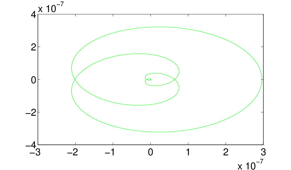
The difference in behaviour on the real line of the two examples can be seen in Figure 4. This is because their partial indices are different. The first example have partial indices $\{0$ , $0\}$ and the second $\{-1$ , $-1\}$ . These partial indices can be computed using the following identity

\left(\begin{array}[]{cc}1&f\\ cf&1\end{array}\right)=\left(\begin{array}[]{cc}1&1\\ c^{1/2}&-c^{1/2}\end{array}\right)\left(\begin{array}[]{cc}1+c^{1/2}f&0\\ 0&1-c^{1/2}f\end{array}\right)\left(\begin{array}[]{cc}\frac{1}{2}&\frac{c^{-1/2}}{2}\\ \frac{1}{2}&\frac{-c^{-1/2}}{2}\end{array}\right).

The errors are compared in Figure 5 and Figure 6. It should be noted that the calculation of “approximate” factors took significantly less computational time than the “exact” factors. Besides the natural difference in magnitude of errors (due to the difference in errors of rational approximations) the shape of the curves are dramatically different. It seems the error in Figure 5 is random and in Figure 6 is systemic. This suggests that in the first example the error in “exact” factorisation is greater than “approximate” factorisation. So the accumulated errors in computing Cauchy integrals is greater than the error in once approximating entries of the matrix function. The reverse is true in the second example.

7. Acknowledgements

I am grateful for support from Prof. Nigel Peake. I benefited from useful discussions with Dr Rogosin, Prof. Speck and Prof. Spitkovsky. Suggestions of the anonymous referees helped to improve this paper. This work was supported by the UK Engineering and Physical Sciences Research Council (EPSRC) grant EP/H023348/1 for the University of Cambridge Centre for Doctoral Training, the Cambridge Centre for Analysis.

References

[1] I. D. Abrahams (1996) Radiation and scattering of waves on an elastic half-space; a non-commutative matrix Wiener-Hopf problem. J. Mech. Phys. Solids 44 (12), pp. 2125–2154. External Links: ISSN 0022-5096, Link, Review MathReviews Cited by: §1, §4, §5.2.
[2] I. D. Abrahams, A. M. J. Davis, and S. G. Llewellyn Smith (2008) Matrix Wiener-Hopf approximation for a partially clamped plate. Quart. J. Mech. Appl. Math. 61 (2), pp. 241–265. External Links: ISSN 0033-5614, Link, Review MathReviews Cited by: §1.
[3] I. D. Abrahams (1997) On the solution of Wiener-Hopf problems involving noncommutative matrix kernel decompositions. SIAM J. Appl. Math. 57 (2), pp. 541–567. External Links: ISSN 0036-1399, Link, Review MathReviews Cited by: §1, §4, §5.2, §5.2.
[4] I. D. Abrahams (2000) The application of Padé approximations to Wiener-Hopf factorization. IMA J. Appl. Math. 65 (3), pp. 257–281. External Links: ISSN 0272-4960, Link, Review MathReviews Cited by: Example 2.
[5] M. C. Câmara, A. B. Lebre, and F.-O. Speck (1992) Meromorphic factorization, partial index estimates and elastodynamic diffraction problems. Math. Nachr. 157, pp. 291–317. External Links: ISSN 0025-584X, Link, Review MathReviews Cited by: Remark 2.1.
[6] A. C. Conceicao, V. G. Kravchenko, and J. C. Pereira (2012) Rational functions factorization algorithm: a symbolic computation for the scalar and matrix cases. Proceedings of CSEI. Cited by: §6.2.
[7] D. G. Crighton (2001) Asymptotic factorization of Wiener-Hopf kernels. Wave Motion 33 (1), pp. 51–65. External Links: ISSN 0165-2125, Link, Review MathReviews Cited by: §1.
[8] V.G. Daniele and R.S. Zich (2014) The Wiener–Hopf method in electromagnetics. Mario Boella Series on Electromagnetism in Information and Communication Series, Institution of Engineering and Technology. External Links: ISBN 9781613530016, Link Cited by: §1, §1, §4, §5.2.
[9] A. S. Fokas, A. R. Its, A. A. Kapaev, and V. Yu. Novokshenov (2006) Painlevé transcendents. Mathematical Surveys and Monographs, Vol. 128, American Mathematical Society, Providence, RI. Note: The Riemann-Hilbert approach External Links: ISBN 0-8218-3651-X, Link, Review MathReviews Cited by: §6.2.
[10] F. D. Gahov and Ju. I. Čerskiĭ Equations of convolution type (in russian). Cited by: §2.2.
[11] S. R. Gennady Mishuris Constructive methods for factorization of matrix-functions. Note: Submitted Cited by: §1, §1.
[12] I. C. Gohberg and M. G. Kreĭn (1960) Systems of integral equations on a half line with kernels depending on the difference of arguments. Amer. Math. Soc. Transl. (2) 14, pp. 217–287. External Links: ISSN 0065-9290, Review MathReviews Cited by: §1.
[13] I. Gohberg, M.A. Kaashoek, and I.M. Spitkovsky (2003) An overview of matrix factorization theory and operator applications. In Factorization and integrable systems, I. Gohberg, N. Manojlovic, and A. dos Santos (Eds.), Operator Theory: Advances and Applications, Vol. 141, pp. 1–102 (English). External Links: Link Cited by: §1, §2.1, §2, Remark 3.1, §3.
[14] C. J. Heaton and N. Peake (2005) Acoustic scattering in a duct with mean swirling flow. J. Fluid Mech. 540, pp. 189–220. External Links: ISSN 0022-1120, Link, Review MathReviews Cited by: §1.
[15] A. A. Khrapkov (1971) The first basic problem for a notch at the apex of an infinite wedge. Internat. J. Fracture Mech. 7, pp. 373–382. External Links: ISSN 0376-9429, Review MathReviews Cited by: §1, §4.
[16] A. V. Kisil (2013) A constructive method for an approximate solution to scalar Wiener–Hopf equations. Proc. R. Soc. Lond. Ser. A Math. Phys. Eng. Sci. 469 (2154), pp. 20120721, 17. External Links: ISSN 1364-5021, Link, Review MathReviews Cited by: §1, §2.2, §2.2, §4, §6.1, Example 2.
[17] A. V. Kisil (2014) On the relationship between a strip wiener-hopf problem and a riemann-hilbert problem. Accepted, IMA J. Appl. Math. Cited by: §6.2.
[18] J. B. Lawrie and I. D. Abrahams (2007) A brief historical perspective of the Wiener-Hopf technique. J. Engrg. Math. 59 (4), pp. 351–358. External Links: ISSN 0022-0833, Link, Review MathReviews Cited by: §1.
[19] G. S. Litvinchuk and I. M. Spitkovskii (1987) Factorization of measurable matrix functions. Operator Theory: Advances and Applications, Vol. 25, Birkhäuser Verlag, Basel. Note: Translated from the Russian by Bernd Luderer, With a foreword by Bernd Silbermann External Links: ISBN 3-7643-1883-X, Link, Review MathReviews Cited by: §1, §1, §2.1, Theorem 3.2, Theorem 3.3.
[20] G. Mishuris and S. Rogosin (2015) Factorization of a class of matrix-functions with stable partial indices. ArXiv e-prints. External Links: 1501.02692 Cited by: §1.
[21] G. Mishuris and S. Rogosin (2014) An asymptotic method of factorization of a class of matrix functions. Proceedings of the Royal Society A: Mathematical, Physical and Engineering Science 470 (2166). External Links: http://rspa.royalsocietypublishing.org/content/470/2166/20140109.full.pdf+html, Link Cited by: §1.
[22] S. Olver and T. Trogdon (2014) Nonlinear steepest descent and numerical solution of Riemann-Hilbert problems. Comm. Pure Appl. Math. 67 (8), pp. 1353–1389. External Links: ISSN 0010-3640, Link, Review MathReviews Cited by: §6.2.
[23] S. Prössdorf and F.-O. Speck (1990) A factorisation procedure for two by two matrix functions on the circle with two rationally independent entries. Proc. Roy. Soc. Edinburgh Sect. A 115 (1-2), pp. 119–138. External Links: ISSN 0308-2105, Link, Review MathReviews Cited by: §5.1, §5.1.
[24] A. D. Rawlins (1997) Two waveguide trifurcation problems. Math. Proc. Cambridge Philos. Soc. 121 (3), pp. 555–573. External Links: ISSN 0305-0041, Link, Review MathReviews Cited by: §4.
[25] L. N. Trefethen (1981) Rational chebyshev approximation on the unit disc. Numerische Mathematik. Cited by: Example 3.
[26] B. Veitch and N. Peake (2008) Acoustic propagation and scattering in the exhaust flow from coaxial cylinders. J. Fluid Mech. 613, pp. 275–307. External Links: ISSN 0022-1120, Link, Review MathReviews Cited by: §1.
[27] B. H. Veitch and I. D. Abrahams (2007) On the commutative factorization of $n\times n$ matrix Wiener-Hopf kernels with distinct eigenvalues. Proc. R. Soc. Lond. Ser. A Math. Phys. Eng. Sci. 463 (2078), pp. 613–639. External Links: ISSN 1364-5021, Link, Review MathReviews Cited by: §1.

$\displaystyle\\|\theta-\tilde{\theta}\\|_{2}$	$\displaystyle\leq$	$\displaystyle\frac{1}{cL}\left\\|\frac{1-\Delta(t)f(t)}{1+\Delta(t)f(t)}-\frac{1-\Delta(t)\tilde{f}(t)}{1+\Delta(t)\tilde{f}(t)}\right\\|_{2}$
	$\displaystyle\leq$	$\displaystyle\frac{2}{cL}\left\\|\frac{\Delta(t)f(t)-\Delta(t)\tilde{f}(t)}{(1+\Delta(t)f(t))(1+\Delta(t)\tilde{f}(t))}\right\\|_{2}$
	$\displaystyle\leq$	$\displaystyle\frac{2}{cd^{2}L}\\|\Delta(t)f(t)-\Delta(t)\tilde{f}(t)\\|_{2},$

$\displaystyle\\|a_{11}-\tilde{a}_{11}\\|_{2}$	$\displaystyle=$	$\displaystyle\\|r_{\pm}(t)\cosh[\Delta(t)\theta_{\pm}(t)]-\tilde{r}_{\pm}(t)\cosh[\Delta(t)\tilde{\theta}_{\pm}(t)]\\|_{2}$
	$\displaystyle\leq$	$\displaystyle\\|r_{\pm}(\cosh[\Delta(t)\theta_{\pm}(t)]-\cosh[\Delta(t)\tilde{\theta}_{\pm}(t)])\\|_{2}$
		$\displaystyle+{}\\|\cosh[\Delta(t)\tilde{\theta}_{\pm}(t)](r_{\pm}-\tilde{r}_{\pm})\\|_{2},$

	$\displaystyle\\|a_{11}-\tilde{a}_{11}\\|_{2}$	$\displaystyle\leq$	$\displaystyle\|r_{\pm}\|\text{ }\|\sinh[\Delta(t)\theta_{\pm}(t)]\|\text{ }\\|\Delta(t)\theta_{\pm}(t)-\Delta(t)\tilde{\theta}_{\pm}(t)\\|_{2}$
			$\displaystyle+{}\|\cosh[\Delta(t)\tilde{\theta}_{\pm}(t)]\|\text{ }\\|(r_{\pm}-\tilde{r}_{\pm})\\|_{2}.$

Stability Analysis of Matrix Wiener–Hopf Factorisation of Daniele–Khrapkov Class and Reliable Approximate Factorisation

Abstract.

Key words and phrases:

1. Introduction

2. Preliminaries

2.1. Wiener–Hopf factorisation

Remark 2.1.

2.2. Scalar Error Estimates

Theorem 2.2 (Additive Estimates in L2L_{2}).

Theorem 2.3 (Multiplicative Estimates in L2L_{2}).

3. Stability of Matrix Wiener–Hopf

Remark 3.1.

Theorem 3.2 (Gohberg – Krein, [19]*§ 6.2).

Theorem 3.3 (Shubin, [19]*§ 6.6).

4. Error estimates in Daniele–Khrapkov Matrices

Lemma 4.1.

Remark 4.2.

Proof.

Lemma 4.3.

Remark 4.4.

Proof.

Theorem 4.5.

Proof.

5. Approximate reducing to extended Daniele–Khrapkov

5.1. Exact reduction to Daniele–Khrapkov Matrices

5.2. Approximate reduction to Daniele–Khrapkov

Remark 5.1.

Example 1.

6. Numerical Results

6.1. Rational approximation

Example 2.

Example 3.

6.2. Numerical Matrix Factorisation

7. Acknowledgements

References

Theorem 2.2 (Additive Estimates in $L_{2}$ ).

Theorem 2.3 (Multiplicative Estimates in $L_{2}$ ).