Diversity-Weighted Portfolios with
Negative Parameter
Thanks: The authors are greatly indebted to Adrian Banner, Robert Fernholz, Thibaut Lienart, Michael Monoyios, Vassilios Papathanakos, Julen Rotaetxe, Johannes Ruf, and an anonymous referee for their very careful reading of the manuscript and their many, insightful, and helpful suggestions.
Abstract
We analyze a negative-parameter variant of the diversity-weighted portfolio studied by Fernholz, Karatzas, and Kardaras (2005, Finance Stoch 9(1):1–27,), which invests in each company a fraction of wealth inversely proportional to the company’s market weight (the ratio of its capitalization to that of the entire market). We show that this strategy outperforms the market with probability one over sufficiently long time-horizons, under a non-degeneracy assumption on the volatility structure and under the assumption that the market weights admit a positive lower bound. Several modifications of this portfolio are put forward, which outperform the market under milder versions of the latter no-failure condition, and one of which is rank-based. An empirical study suggests that such strategies as studied here have indeed the potential to outperform the market and to be preferable investment opportunities, even under realistic proportional transaction costs.
1 Introduction
Stochastic Portfolio Theory offers a relatively novel approach to portfolio selection in stock markets, aiming – among other things – to construct portfolios which outperform an index, or benchmark portfolio, over a given time-horizon with probability one, whenever this might be possible. The reader is referred to R. Fernholz’s monograph (Fernholz, 2002), and to the more recent overview by Fernholz and Karatzas (2009). In Fernholz et al. (2005) such outperforming portfolios have been shown to exist over sufficiently long time-horizons, in market models which satisfy certain assumptions; namely, those of weak diversity and non-degeneracy.
One such investment strategy is the so-called diversity-weighted portfolio. This re-calibrates the weights of the market portfolio, by raising them all to some given power and then re-normalizing; see Fernholz et al. (2005). We study here a variant of this strategy, namely, a diversity-weighted portfolio with negative parameter . This strategy invests in each company a proportion of wealth that is inversely proportional to the ratio of the company’s capitalization to the capitalization of the entire market (this ratio is called the company’s market weight). As a result, the strategy sells the company’s stock as its value increases, and buys it as its value decreases.
1.1 Preview
We set up the model and introduce the necessary definitions in Section 2. Our first main result is that this negative-parameter diversity-weighted portfolio also outperforms the market over long time-horizons, but now under a no-failure condition. This postulates that all market weights are uniformly bounded from below by a positive constant — see Section 3. The no-failure condition is stronger than diversity.
A rank-based modification of this portfolio, which only invests in small-capitalization stocks, is then shown in Section 4 to outperform the market, also under this assumption of “no-failure”. For certain positive parameters , this rank-based portfolio outperforms the market under a milder and more realistic condition, namely that of limited-failure. This condition posits a uniform lower bound on market weights only for the largest firms by capitalization, with the total number of equities in the market.
We present two additional results in Section 5. The first shows that the negative-parameter diversity-weighted portfolio outperforms its positive-para-meter version under an additional boundedness assumption on the covariation structure of the market; this posits that the eigenvalues of the covariance matrix in the underlying Itô model are bounded from above, uniformly in time. Our second result studies a composition of these two diversity-weighted portfolios and shows that, under the condition of diversity, this “mix” almost surely performs better than the market over sufficiently long time-horizons.
We carry out an empirical study of the constructed portfolios in Section 6, demonstrating that our adjustments of the diversity-weighted portfolio would have outperformed quite considerably the S&P 500 index, if implemented on the index constituents over the 25 year period between January 1, 1990 and December 31, 2014. In this study we incorporate 0.5% proportional transaction costs, delistings due to bankruptcies, mergers and acquisitions, and distributions such as dividends. We compute the relative returns of our portfolios over this period, as well as the Sharpe ratios relative to the market index. We discuss the results and possible future work in Section 7.
2 Preliminaries
2.1 The Model
Our market model is the standard one of Stochastic Portfolio Theory (Fernholz, 2002), where the stock capitalizations are modeled as Itô processes. Namely, the dynamics of the stock capitalization processes are given by
| (1) |
here are independent standard Brownian motions with , and are the initial capitalizations. We assume all processes to be defined on a probability space , and adapted to a filtration that satisfies the usual conditions and contains the filtration generated by the “driving” Brownian motions.
The processes of rates of return and of volatilities are -progressively measurable and assumed to satisfy the integrability condition
| (2) |
as well as the non-degeneracy condition
| (ND) |
2.2 Relative Arbitrage
We study investments in the equity market described by (1) using portfolios. These are -valued and -progressively measurable processes , where stands for the proportion of wealth invested in stock at time .
We restrict ourselves to long-only portfolios. These invest solely in the stocks, namely
| (3) |
in particular, there is no money market. The corresponding wealth process of an investor implementing is seen to evolve as follows (we normalize the initial wealth to 1):
| (4) |
We shall measure performance, for the most part, with respect to the market index. This is the wealth process that results from a buy-and-hold portfolio, given by the vector process of market weights
| (5) |
Definition 1.
A relative arbitrage with respect to a portfolio over the time-horizon , for a real number , is a portfolio such that
| (6) |
An equivalent way to express this notion, is to say that the portfolio outperforms portfolio over the time-horizon .
We call this relative arbitrage strong, if in fact ; and sometimes we express this by saying that the portfolio outperforms the portfolio strongly over the time-horizon . ∎
We introduce the -valued covariation process and, writing for the th unit vector in , the relative covariances
| (7) |
Finally, we define the excess growth rate of a portfolio as
| (8) |
We shall use the reverse-order-statistics notation, defined recursively by
| (9) | ||||
for any -valued process . Here ties are resolved lexicographically, always in favor of the lowest index . Thus we have
| (10) |
The non-degeneracy condition (ND) implies, on the strength of Lemma 3.4 in Fernholz and Karatzas (2009) (originally proved in the Appendix of Fernholz et al. (2005)), that for any long-only portfolio we have with probability one:
| (11) |
2.3 Functionally-Generated Portfolios
A particular class of portfolios, called functionally-generated portfolios, was introduced and studied by Fernholz (1999).
Consider a function , where is an open neighborhood of
| (12) |
and such that is bounded on for . Then is said to be the generating function of the portfolio given, for , by
| (13) |
Here and throughout the paper, we write for the partial derivative with respect to the variable, and for the second partial derivative with respect to the and variables. Theorem 3.1 of Fernholz (1999) asserts that the performance of the wealth process corresponding to , when measured relative to the market, satisfies the decomposition (often referred to as “Fernholz’s master equation”)
| (14) |
The quantity
| (15) |
is called the drift process of the portfolio .
2.4 Diversity-Weighted Portfolios
We consider now the diversity-weighted portfolio with parameter , defined as in (4.4) of Fernholz et al. (2005):
| (16) |
One condition that was shown to be sufficient for the existence of relative arbitrage in the model (1), under the condition (ND), is that of diversity (see Corollary 2.3.5 and Example 3.3.3 of Fernholz (2002)). This posits that no single company’s capitalization can take up more than a certain proportion of the entire market.
More formally, a market is said to be diverse over the time-horizon , for some real number , if
| (D) |
Models of the form (1), which satisfy the property (D) and admit local martingale deflators, were explicitly shown to exist in Remark 6.2 of Fernholz et al. (2005). Other constructions have been proposed by Osterrieder and Rheinländer (2006) and Sarantsev (2014). Fernholz et al. (2005, see Eq. (4.5)) showed that the portfolio (16) outperforms the market index strongly, in markets satisfying (ND) and (D), for any , and over time-horizons with
| (17) |
In Theorem 1 below, we show that a similar property holds for the diversity-weighted portfolio with negative parameter , in markets with the following no-failure condition:
| (NF) |
We note that this condition implies diversity with parameter
3 Main Result
Here is the main result of this paper.
Theorem 1.
Proof.
We apply the theory of functionally-generated portfolios as in Section 2.3. For any , it is checked that the portfolio (16) is generated by the function
| (20) |
We apply the method of Lagrange multipliers to maximize this function for subject to ; this gives We may therefore write that, under (NF), the generating function admits the lower and upper bounds
| (21) |
Hence, for any , we have the lower bound
| (22) |
a negative number. Using assumption (NF) and the lower bound from (21), we obtain
| (23) |
where the last (strict) inequality follows from (18). In conjunction with (23), the inequality (11) gives
| (24) |
Finally, straightforward computation shows that the drift process of the portfolio (16), as defined in (15), is equal for all to
| (25) |
We apply now (25), (22) and (24) to Fernholz’s master equation (14), and conclude that the relative performance of over , with respect to the market, is given by
| (26) | ||||
provided satisfies (19). Hence the portfolio outperforms the market strongly over sufficiently long time-horizons , as indicated in (19). ∎
4 Rank-Based Variants
Real markets typically do not satisfy the (NF) assumption (as stocks can crash), so it is desirable to weaken this condition of Theorem 1. One possible modification of (NF), is to posit that “no-failure” only holds for the stocks ranked highest by capitalization, for some fixed , namely
| (LF) |
We call this condition (LF) the limited-failure condition, as it postulates that no more than companies will “go bankrupt” by time . In this context, bankruptcy of company during the time-horizon is defined as the event such that . We also note that (LF) implies the diversity condition with parameter
Remark 1.
As was noted by V. Papathanakos (private communication), the diversity condition (D) with parameter in turn implies (LF) with parameters
| (27) |
with the largest integer less than or equal to . To see this, we note that, as long as , for , we have the implication
| (28) |
We identify the inequality on the right hand side of (28) as a version of (LF). The largest integer for which this lower bound is positive, is , giving (27). ∎
4.1 A Diversity-Weighted Portfolio of Large Stocks
Under the assumption (LF), one can attempt to construct a relative arbitrage using a variant (introduced in Example 4.2 of Fernholz (2001)) of the diversity-weighted portfolio with parameter which only invests in the highest-ranked stocks (and thus naturally avoids investing in “crashing” stocks), namely:
| (29) |
Here, is the index of the stock ranked th at time (with ties resolved “lexicographically” once again, by choosing the lowest index), so that .
We shall denote by the semimartingale local time accumulated at the origin, over the time-interval , by the continuous, non-negative semimartingale
| (30) |
Definition 2.
Let us consider the local times at the origin of all continuous, nonnegative semimartingales of the form
and call them “higher-order collision local times”. ∎
We shall assume throughout this section the following:
Assumption 1.
All higher-order collision local times vanish. ∎
The reader should consult Banner and Ghomrasni (2008) for general theory on ranked semimartingales, as well as Ichiba et al. (2011) for sufficient conditions that ensure the evanescence of such higher-order collision local times, as posited in Assumption 1.
When attempting to construct a relative arbitrage with the portfolio (29), one encounters a problem. To wit: an application of Theorem 3.1 of Fernholz (2001) asserts that the following master equation holds for this rank-based portfolio:
| (31) | ||||
with the generating function of ; compare with (26). Due to the unbounded nature of semimartingale local time, the final term in (31) (referred to as “leakage” by Fernholz (2001)) admits no obvious almost sure bound. Thus there is no lower bound on the market-relative performance of that holds under reasonable conditions.
Since in real markets this local time term is typically small, we do still expect this portfolio to have a good performance, and therefore include it in our empirical study — see Section 6.
4.2 A Diversity-Weighted Portfolio of Small Stocks
Let us then fix , and define a small-stock diversity-weighted portfolio by
| (32) |
With this new dispensation, the local time term in (31) changes sign for (see equation (38) below) and the problems mentioned in the previous subsection disappear. In fact, we can show that the new portfolio in (32) outperforms the market under the assumptions (ND), (LF), for certain positive values of the parameter ; as well as under the assumptions (ND), (NF), when is within an appropriate range of negative values.
Proposition 1.
We place ourselves in the context of the market model (1), and under Assumption 1 and the condition (ND).
(i) If the condition (LF) also holds, the small-stock diversity-weighted portfolio of (32) with parameter
| (33) |
is a strong relative arbitrage with respect to the market over the time-horizon , provided that
| (34) |
(ii) If (NF) also holds, the small-stock diversity-weighted portfolio of (32) with parameter
| (35) |
is a strong arbitrage relative to the market over the time-horizon , provided
| (36) |
Proof.
The portfolio (32) is generated by the function
| (37) |
a rank-based variant of (20). In a manner analogous to (31), Theorem 3.1 of Fernholz (2001) implies the following master equation for the performance of our small-stock portfolio:
| (38) | ||||
We note the change of sign for the last term, when juxtaposed with the analogue (31) of this equation for the large-stock portfolio in (29).
Case (i):
With as in (33), we have
| (39) |
Recalling (LF) and , we have the following bounds
| (40) | ||||
for the generating function , and lead to the lower bound
| (41) |
Note that, using the lower bound in (40) and , , we obtain
| (42) |
where the last bound follows from the inequalities in (39).
The non-degeneracy condition (ND) now gives
| (43) |
in conjunction with (11) and (42). Whereas the nonnegativity of coupled with the nondecrease of the local time shows that
| (44) |
We use this and apply (41) and (43) to the rank-based master equation (38), to obtain
| (45) | ||||
if and only if as defined in (34). We conclude that, under these conditions, strongly outperforms the market over the horizon .
Case (ii):
With and under the condition (NF), we have the following bounds
| (46) |
For the first inequality, we have used the simple fact that holds for . Whereas, from (35), we have
| (47) |
by analogy with (23). The inequalities (46) lead to the lower bound
| (48) |
and the non-degeneracy condition (ND), in conjunction with (11) and the upper bound (47) on the largest portfolio weight , give
| (49) |
Again, we use (44) and apply (48) and (49) to the master equation (38), to obtain
| (50) | ||||
provided as defined in (36).
Hence this small-stock, negative-parameter portfolio , outperforms the market over the horizon . ∎
5 Further Considerations
We present now some other results, the first of which shows that the diversity-weighted portfolio (16) with is outperformed by its negative-para-meter counterpart under sufficient conditions. We also study a particular combination of these two types of diversity-weighted portfolios, showing that it outperforms a non-degenerate diverse market — see Proposition 3 further below.
5.1 Negative vs. Positive Parameter
In the following Proposition 2, besides (ND) we will impose also an upper bound on the eigenvalues of the covariance matrix , in the form of the bounded variance assumption:
| (BV) |
By Lemma 3.5 of Fernholz and Karatzas (2009), the bounded variance condition (BV) implies that for long-only portfolios we have the almost sure inequality
| (51) |
Proposition 2.
The diversity-weighted portfolio with negative parameter
is then a strong arbitrage relative to the diversity-weighted portfolio with positive parameter
| (52) |
over any horizon of length
| (53) |
Here the positive constant is defined as
| (54) |
Proof.
To simplify notation a bit, we write and for and , respectively. Note that for the inequalities in (21) reverse, i.e.,
| (55) |
which again gives the lower bound of (22) for . Using (51) with the observation , we get that
| (56) |
Hence, recalling (25), we see that by virtue of (55) and (56) the master equation (14) for leads to the upper bound
| (57) |
Combining (26) and (57), we find that
| (58) | ||||
provided that
| (59) |
Here, the constant is given by (54). An easy calculation shows that (52) implies , whereas the last inequality in (59) comes from . It follows that the first inequality in (59) is equivalent to the condition posited in (53), and that in this case outperforms strongly over the time-horizon . ∎
Proposition 2 shows that, as long as the diversity-weighted portfolio is “sufficiently similar” to the market portfolio (and thus “far enough” from ), it is outperformed strongly, over sufficiently long time-horizons, by the diversity-weighted portfolio with negative parameter – provided, of course, that the aforementioned conditions on the volatility structure and non-failure of stocks hold.
Remark 2.
Compared to (D), the stronger (NF) assumption implies a possibly shorter minimal time horizon than that of (17), over which the diversity-weighted portfolio with parameter is guaranteed strongly to outperform the market. Namely, the fact that together with (55), implies that
| (60) |
Recall from the end of Section 2.4 that (NF) implies diversity (D) with parameter . It follows from (17), and using an argument similar to that in the proof of Theorem 1, that the positive-parameter diversity-weighted portfolio is a strong arbitrage relative to the market over horizons , with
| (61) |
This is an improvement of (17) if and only if . ∎
5.2 Mixing
Since the no-failure assumption (NF) does not hold in real markets, it is of interest to find variants of (16) which exhibit similar performance, but require weaker assumptions. The rank-based variant in Proposition 1 is one attempt at this; Proposition 3 right below is another.
Proposition 3.
Proof.
The portfolio (62) is generated by the function , with the generating functions of as in (20); let be their drift processes as in (25).
The drift process of the composite portfolio is then
| (65) |
the final step follows from (25). We note that
| (66) |
as this holds for any long-only portfolio by Lemma 3.3 of Fernholz and Karatzas (2009), which together with the observation that allows us to obtain the bound
| (67) |
We note the simple bounds
| (68) |
and that the lower bound in (21) holds even without (NF), so now
| (69) |
Using the lower bound from (68), and the upper bound from (69), we assert that
| (70) |
One can easily see that in the positive-parameter diversity-weighted portfolio, one’s proportion of wealth invested relative to the market portfolio is diminished for large-cap stocks, and increased for small-capitalization stocks; therefore
| (71) |
The non-degeneracy condition (ND) implies (11), which by (71) and the diversity assumption (D) leads to
| (72) |
We have shown that the long-only portfolio (62) outperforms strongly the market over sufficiently long time-horizons, under the assumptions of non-degeneracy and diversity. This is a property that the portfolio also has on its own, as proved in the Appendix of Fernholz et al. (2005).
We remark also that, since the “threshold” of (64) is strictly decreasing in , and the lower bound (73) is strictly increasing in for fixed , our result becomes stronger the closer the negative parameter gets to the origin. As we take , we recover the well-known result that is a strong arbitrage relative to the market.
Remark 3.
The statement of Proposition 3 can be strengthened, by weakening the diversity condition (D) to that of weak diversity over the horizon . This notion is defined in equation (4.2) of Fernholz et al. (2005) as
| (WD) |
Under this weaker assumption, it is straightforward to see that the following modification of (72) will hold, thus maintaining the validity of the proof:
| (74) |
∎
5.3 Arbitrary Time Horizons
We should note here that, since both the (NF) and (LF) conditions imply diversity, by Lemma 8.1 and Example 8.3 of Fernholz et al. (2005) it follows that short-term relative arbitrage exists. That is, using the “mirror portfolios” of Fernholz, Karatzas and Kardaras, one can construct a portfolio which outperforms the market over any time-horizon .
5.4 Two Portfolios with a Threshold
We mention briefly two other variants of the portfolio (16) with , which exhibit similar behavior for mid- and upper-range market weights (in the sense that they invest in stocks which decrease in value relative to the market, and sell stock when a company’s market weight increases), but start selling stock once a firm’s market weight falls below a certain threshold. The idea behind this threshold is that it represents a value below which the investor fears bankruptcy of the firm, and wishes to liquidate the position in the firm so as to minimize losses. The two portfolios we propose have weights
| (75) |
and
| (76) |
Here, and are all positive constants; the threshold values below which the portfolio weights become increasing functions of market weights are and , respectively. So far, our results regarding these portfolios remain restricted to empirical ones (see Section 6). A theoretical result for the portfolio might follow in a way similar to that of Proposition 1 in Banner and Fernholz (2008).
6 Empirical Results
We test the validity and applicability of our theoretical results by conducting an empirical study of the performance of our portfolios using historical market data. More precisely, we back-test by investing according to the portfolios studied here in the daily constituents of the S&P 500 index for consecutive trading days between 1 January 1990 and 31 December 2014. We obtain these data from the Compustat and CRSP data sets (these data sets are obtainable from the website http://wrds-web.wharton.upenn.edu/wrds/). We have incorporated dividends and delistings such as mergers, acquisitions and liquidations.
We aim to simulate as realistically as possible the wealth evolution of an investor implementing our portfolios without any additional information, and as such impose on each trade proportional transaction costs equal to 0.5% of the total absolute value traded. We rebalance the portfolio using a simple Total Variance criterion, that is, we only rebalance when the total variance “distance”
| (77) |
between the target portfolio and the portfolio becomes larger than a certain threshold, which we determine empirically by trial-and-error — that is, we simply try several threshold values for each portfolio, and select the one which gives the highest return over the entire holding period for that particular strategy. Here, is the vector of proportions of wealth invested in stocks obtained when the investor does not rebalance at time , that is
where is the portfolio that was actually implemented in the previous time step.
We use R to program our simulations — the code is available upon request. We summarize our findings in Table 1, which displays the average annual relative returns in excess of the market (denoted “Market-RR”), and the Sharpe ratios of our portfolios over the entire 25-year period that we use; the latter is computed as
| (78) |
Here, are the daily returns of the portfolio , with mean , namely
| (79) |
and the sample standard deviation StdDev is defined as follows for any sequence of numbers with average :
| (80) |
Moreover, we compute the following measure of performance for each portfolio:
| (81) |
that is, the total growth rate divided by the sample standard deviation. The former is estimated as
| (82) |
Figure 1 showcases the wealth processes corresponding to our portfolios.
| Portfolio | Threshold | Market-RR | Sharpe Ratio | |
|---|---|---|---|---|
| N/A | 0% | 0.60477 | 8.1678 | |
| 0.0005 | 2.2331% | 0.70428 | 9.7127 | |
| 0.0022 | 1.6125% | 0.76766 | 10.949 | |
| 0.0015 | 4.9655% | 0.78558 | 10.910 | |
| 0.0025 | 2.5778% | 0.76979 | 10.873 | |
| 0.0001 | 0.9578% | 0.64713 | 8.8215 | |
| 0.0100 | 1.7645% | 0.67412 | 9.2114 | |
| 0.0022 | 1.6125% | 0.76766 | 10.949 | |
| 0.0020 | 3.6336% | 0.68160 | 9.0796 | |
| 0.0002 | 1.8701% | 0.67919 | 9.2920 |
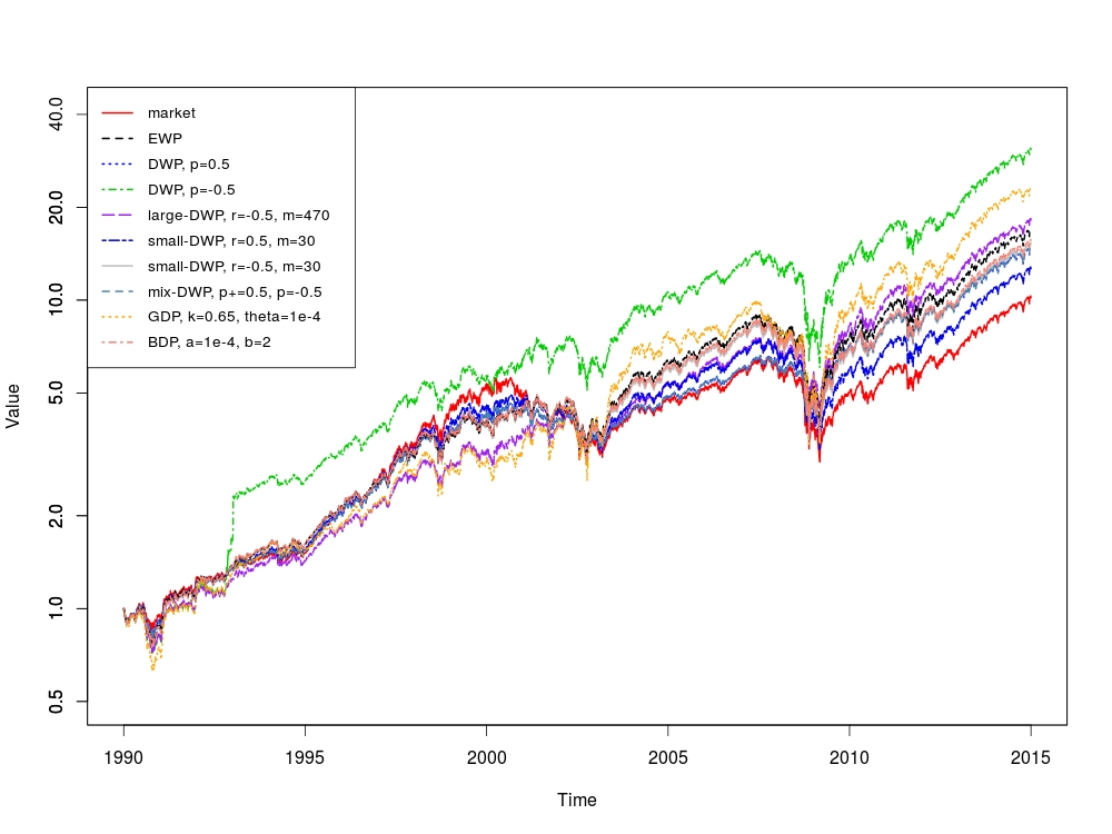
From Table 1 and Figure 1, we can see that all portfolios outperform the market by quite a margin (however, only after the year 2000), both in terms of the market-relative return, as well as the Sharpe Ratio. We also note that the simulated realizations of wealth processes are much more volatile than that of the market; the portfolios seem to exploit market growth much better, but also lose value more quickly when the market does poorly. Moreover, the negative-parameter portfolios we study appear to perform better than their positive-parameter versions over the period studied. The reader will notice that the positive-parameter portfolio with , and the mixing portfolio , give identical results, which is because the weight (63) of the positive-parameter diversity-weighted portfolio is always very near 1 (namely ). Finally, we wish to stress that the above portfolio and threshold parameters were optimized only heuristically, and therefore there is considerable room for improvement (that is, through more systematic optimization) — the performance of the portfolios is quite sensitive to these parameters, as well as the level of transaction costs. Our empirical study is therefore merely a demonstration of potential outperformance of the market with the portfolios studied for a small investor.
7 Discussion and Suggestions for Future Research
We wish to point out that all of our results require certain assumptions on the volatility structure of the market, as well as on the behavior of the market weights. The no-failure condition (NF) definitely does not hold in real markets, since typically some companies do crash. The weaker (LF) assumption is an improvement on this, and can be argued to hold for not too close to — although, to the authors’ knowledge, there is no mechanism holding this in place, as there is for the diversity assumption (D) which can be imposed by anti-trust regulation. In this regard, see Strong and Fouque (2011), as well as the recent paper by Karatzas and Sarantsev (2014) in which the number of companies is allowed to fluctuate – due to both splits and mergers of companies.
It has been raised by V. Papathanakos (private communication) that from a practitioner’s point of view, there are several restrictions on the implementation of negative-parameter diversity-weighted portfolios on a large scale. One of these is that one typically demands that no position owns more than, say, 1% of the outstanding shares of a security; our portfolios strongly invest in small stocks. Another constraint is related to liquidity: regular rebalancing in a predictable way (which is implied by all functionally-generated portfolios) incurs very high transaction costs. It would be useful to model these phenomena and their influence on portfolio performance.
More generally, it would be of great interest to develop a theory of transaction costs in the framework of Stochastic Portfolio Theory, which would allow one to improve upon, or even optimize over, rebalancing rules given a certain portfolio. A first attempt at this was made by (Fernholz, 2002, Section 6.3), where R. Fernholz estimates the turnover in a diversity-weighted portfolio.
Another idea is to replace the almost sure assumptions (D), (LF), and (NF), by probabilistic versions of these assumptions, where the corresponding bounds on market weights hold with a probability close to but smaller than 1. It would be interesting to see whether probabilistic relative arbitrages could be constructed, which have a certain “likelihood of outperforming” the market — see Bayraktar et al. (2012) for a first study in this direction.
One could also incorporate additional information on expected drifts and bankruptcies, to improve the simple portfolios set forth in this paper. The approach by Pal and Wong (2013) might be applied to achieve this. Moreover, it would be of interest to develop methods for finding the optimal relative arbitrage within the class of functionally-generated portfolios; an attempt at this was made in Pal and Wong (2014), and for more general strategies in Fernholz and Karatzas (2010) and Fernholz and Karatzas (2011). Limitations on the existence of relative arbitrages with respect to certain portfolios have been established in the recent paper Wong (2015).
Acknowledgements
Wharton Research Data Services (WRDS) was used in preparing the data for this paper. This service and the data available thereon constitute valuable intellectual property and trade secrets of WRDS and/or its third-party suppliers.
References
- Banner and Fernholz [2008] Adrian D. Banner and Daniel Fernholz. Short-term relative arbitrage in volatility-stabilized markets. Ann. Finance, 4:445–454, 2008.
- Banner and Ghomrasni [2008] Adrian D. Banner and Raouf Ghomrasni. Local times of ranked continuous semimartingales. Stochastic Processes and their Applications, 118(7):1244–1253, 2008.
- Bayraktar et al. [2012] Erhan Bayraktar, Yu-Jui Huang, and Qingshuo Song. Outperforming the market portfolio with a given probability. Ann. Appl. Probab., 22(4):1465–1494, 2012.
- Fernholz and Karatzas [2010] Daniel Fernholz and Ioannis Karatzas. On optimal arbitrage. Ann. Appl. Probab., 20(4):1179–1204, 2010.
- Fernholz and Karatzas [2011] Daniel Fernholz and Ioannis Karatzas. Optimal arbitrage under model uncertainty. Ann. Appl. Probab., 21(6):2191–2225, 2011.
- Fernholz [1999] Robert Fernholz. Portfolio generating functions. Quantitative Analysis in Financial Markets, River Edge, NJ. World Scientific, 1999.
- Fernholz [2001] Robert Fernholz. Equity portfolios generated by functions of ranked market weights. Finance Stoch., 5:469–486, 2001.
- Fernholz [2002] Robert Fernholz. Stochastic Portfolio Theory. Springer, 2002.
- Fernholz and Karatzas [2009] Robert Fernholz and Ioannis Karatzas. Stochastic portfolio theory: A survey. In Alain Bensoussan and Qiang Zhang, editors, Handbook of Numerical Analysis. Vol. XV. Special volume: mathematical modeling and numerical methods in finance, volume 15 of Handbook of Numerical Analysis. Elsevier/North-Holland, Amsterdam, 2009.
- Fernholz et al. [2005] Robert Fernholz, Ioannis Karatzas, and Constantinos Kardaras. Diversity and relative arbitrage in equity markets. Finance Stoch., 9(1):1–27, 2005.
- Ichiba et al. [2011] Tomoyuki Ichiba, Vassilios Papathanakos, Adrian Banner, Ioannis Karatzas, and Robert Fernholz. Hybrid Atlas models. Ann. Appl. Probab., 21(2):609–644, 2011.
- Karatzas and Sarantsev [2014] Ioannis Karatzas and Andrey Sarantsev. Diverse market models of competing Brownian particles with splits and mergers. arXiv preprint arXiv:1404.0748, 2014.
- Osterrieder and Rheinländer [2006] Jörg R. Osterrieder and Thorsten Rheinländer. Arbitrage opportunities in diverse markets via a non-equivalent measure change. Ann. Finance, 2:287–301, 2006.
- Pal and Wong [2013] Soumik Pal and Ting-Kam Leonard Wong. Energy, entropy, and arbitrage. arXiv preprint arXiv:1308.5376, 2013.
- Pal and Wong [2014] Soumik Pal and Ting-Kam Leonard Wong. The geometry of relative arbitrage. arXiv preprint arXiv:1402.3720, 2014.
- Sarantsev [2014] Andrey Sarantsev. On a class of diverse market models. Ann. Finance, 10(2):291–314, 2014.
- Strong and Fouque [2011] Winslow Strong and Jean-Pierre Fouque. Diversity and arbitrage in a regulatory breakup model. Ann. Finance, 7:349–374, 2011.
- Wong [2015] Ting-Kam Leonard Wong. Optimization of relative arbitrage. Ann. Finance, pages 1–38, 2015.