跳到论文正文
W Papers独立论文阅读器 arXiv:1504.00896 论文正文 计算阅读时间 · 0%
引用这篇论文根据当前论文元数据生成,正式投稿前建议核对。


License: arXiv.org perpetual non-exclusive license
arXiv:1504.00896v3 [math.AT] 27 Sep 2017

Rational homology and homotopy of
high dimensional string linksThanks: The second author is partially supported by the Simons Foundation “Collaboration grant for mathematicians”, award ID: 519474.

Paul Arnaud Songhafouo Tsopméné Affiliation: Victor Turchin
Abstract

Arone and the second author showed that when the dimensions are in the stable range, the rational homology and homotopy of the high dimensional anologues of spaces of long knots can be calculated as the homology of a direct sum of finite graph-complexes that they described explicitly. They also showed that these homology and homotopy groups can be interpreted as the higher order Hochschild homology also called Hochschild-Pirashvili homology. In this paper, we generalize all these results to high dimensional analogues of spaces of string links.

The methods of our paper are applicable in the range when the ambient dimension is at least twice the maximal dimension of a link component plus two, which in particular guarantees that the spaces under the study are connected. However, we conjecture that our homotopy graph-complex computes the rational homotopy groups of links spaces always when codimension is greater than two, i.e. always when the Goodwillie-Weiss calculus is applicable. Using Haefliger’s approach to calculate the groups of isotopy classes of higher dimensional links, we confirm our cojecture at the level of π0\pi_{0}.

0 Introduction

In this paper we further develop the connection between the study of embedding spaces, operad theory, and graph-complexes. Our results are partially influenced by Bar Natan’s work [4], where he describes the space dual to weight systems (counting Vassiliev invariants) of string links in ℝ3\mathbb{R}^{3} as a space of unitrivalent graphs modulo A​SAS and I​H​XIHX relations, with univalent vertices being colored by the components of the links, see also [8, Section 5.10] for more details. This space is built from the components of the modular envelop 𝐌𝐨𝐝⁡(ℒ​i​e)\mathbf{Mod}({{\mathcal{L}}ie}) of the operad of Lie algebras [28]. One of our main results says that the rational homotopy of the space of higher-dimensional string links is described as the homology of a graph-complex similarly built from the components of the modular envelop of ℒ∞{\mathcal{L}}_{\infty}. In particular Bar Natan’s space of unitrivalent graphs with colored univalent vertices appears as the bottom degree homology of our complexes. The approach that we use is from our previous works [2, 3, 45]. It is applicable only when codimension is high enough to guarantee that the spaces in question are connected. However, we conjecture that the same result holds requiring only codimension >2>2. To justify this conjecture we express the rational Haefliger groups of isotopy classes of higher-dimensional links [27] as spaces of unitravalent trees with leaves colored by the components of the links (similarly as Bar Natan’s space). We show that this is exactly the degree zero homology of the corresponding homotopy graph-complexes. In particular unitrivalent graphs of loop order ≥1\geq 1 are also present in the homology of these graph-complexes but they appear in positive degrees.

In this paper we produce two different graph-complexes computing the rational homotopy of spaces of string links. One of them is built from the components of 𝐌𝐨𝐝⁡(ℒ∞)\mathbf{Mod}({\mathcal{L}}_{\infty}) and another one has building blocks desrcibed in terms of the homology of configuration spaces of points in Euclidean spaces. Both complexes resemble those appearing in the Bott-Taubes type integration, see for example [7, 42, 43, 51]. The obtained complexes all split into a direct sum of finite complexes. In the follow up paper [46], we compute the generating function of the Euler characteristics of the summands of these complexes (both for the homology and homotopy). As a byproduct result in [46], we compute the supercharacter of the symmetric group action on the positive arity components of 𝐌𝐨𝐝⁡(ℒ∞)\mathbf{Mod}({\mathcal{L}}_{\infty}).

Let dd be the dimension of the ambient space. Let r≥1r\geq 1, and let m1,⋯,mr≥1m_{1},\cdots,m_{r}\geq 1 be rr integers. A high-dimensional string link of rr strands is a smooth embedding f:∐i=1rℝmi↪ℝdf\colon\coprod_{i=1}^{r}\mathbb{R}^{m_{i}}\hookrightarrow\mathbb{R}^{d} that coincides outside a compact set with a fixed embedding ι:∐i=1rℝmi↪ℝd\iota\colon\coprod_{i=1}^{r}\mathbb{R}^{m_{i}}\hookrightarrow\mathbb{R}^{d} affine on each component. When rr is understood we will just say high-dimensional string link. The space of high-dimensional string links, denoted Embc​(∐i=1rℝmi,ℝd)\mbox{Emb}_{c}(\coprod_{i=1}^{r}\mathbb{R}^{m_{i}},\mathbb{R}^{d}), is the collection of all high-dimensional string links endowed with the weak 𝒞∞\mathcal{C}^{\infty}-topology. Similarly, we define the space Immc​(∐i=1rℝmi,ℝd)\mbox{Imm}_{c}(\coprod_{i=1}^{r}\mathbb{R}^{m_{i}},\mathbb{R}^{d}) of smooth immersions ∐i=1rℝmi↬ℝd\coprod_{i=1}^{r}\mathbb{R}^{m_{i}}\looparrowright\mathbb{R}^{d} that coincide outside a compact set with ι\iota. By definition, there is an inclusion Embc​(∐i=1rℝmi,ℝd)↪Immc​(∐i=1rℝmi,ℝd)\mbox{Emb}_{c}(\coprod_{i=1}^{r}\mathbb{R}^{m_{i}},\mathbb{R}^{d})\hookrightarrow\mbox{Imm}_{c}(\coprod_{i=1}^{r}\mathbb{R}^{m_{i}},\mathbb{R}^{d}), and its homotopy fiber over ι\iota, denoted Emb¯c​(∐i=1rℝmi,ℝd)\overline{\mathrm{Emb}}_{c}(\coprod_{i=1}^{r}\mathbb{R}^{m_{i}},\mathbb{R}^{d}), is the space under our study in this paper. The case r=1r=1 was extensively studied in [2] and [3] by Arone and the second author. They obtain the Hodge decomposition in the rational homology H∗​(Emb¯c​(ℝm,ℝd),ℚ)H_{*}(\overline{\mbox{Emb}}_{c}(\mathbb{R}^{m},\mathbb{R}^{d}),\mathbb{Q}) and in the rational homotopy ℚ⊗π∗​Emb¯c​(ℝm,ℝd)\mathbb{Q}\otimes\pi_{*}\overline{\mbox{Emb}}_{c}(\mathbb{R}^{m},\mathbb{R}^{d}), d>2​m+1d>2m+1. Then they explicitly describe graph-complexes computing H∗​(Emb¯c​(ℝm,ℝd),ℚ)H_{*}(\overline{\mbox{Emb}}_{c}(\mathbb{R}^{m},\mathbb{R}^{d}),\mathbb{Q}) and ℚ⊗π∗​Emb¯c​(ℝm,ℝd)\mathbb{Q}\otimes\pi_{*}\overline{\mbox{Emb}}_{c}(\mathbb{R}^{m},\mathbb{R}^{d}).

Because of the high codimension, the space Emb¯c​(∐i=1rℝmi,ℝd)\overline{\mathrm{Emb}}_{c}(\coprod_{i=1}^{r}\mathbb{R}^{m_{i}},\mathbb{R}^{d}) is connected and moreover its homotopy type does not depend on the choice of the fixed affine embedding ι\iota. In particular we can choose ι\iota in a way that all connected components of the fixed unlink are parallel to a given line. Concatenation of links along the direction of this line defines an HH-space structure on Emb¯c​(∐i=1rℝmi,ℝd)\overline{\mathrm{Emb}}_{c}(\coprod_{i=1}^{r}\mathbb{R}^{m_{i}},\mathbb{R}^{d}), which implies that the rational homology of Emb¯c​(∐i=1rℝmi,ℝd)\overline{\mathrm{Emb}}_{c}(\coprod_{i=1}^{r}\mathbb{R}^{m_{i}},\mathbb{R}^{d}) is a cofree cocommutative coalgebra cogenerated by the rational homotopy. The same is true for the graph-complexes that we study.

In order to describe our graph-complexes, we need Theorem 0.1 below, which is a generalization of [2, Theorem 1.3]. Before stating Theorem 0.1, we will recall two notions. The first one is that of right Ω\Omega-modules. Let Ω\Omega be the category of finite unpointed sets whose morphisms are surjections. A right Ω\Omega-module is a contravariant functor from Ω\Omega to any given category. We denote by RmodΩ\underset{\Omega}{\mbox{Rmod}} the category of right Ω\Omega-modules of chain complexes over ℚ\mathbb{Q}. Abusing notation let i∈Ωi\in\Omega denote the set {1,…,i}\{1,\ldots,i\}. The category of right Ω\Omega-modules of ℚ\mathbb{Q}-vector spaces is an abelian category with the set of projective generators ℚ​[homΩ​(i,−)]\mathbb{Q}[\mathrm{hom}_{\Omega}(i,-)], i≥0i\geq 0. Using this fact we endow RmodΩ\underset{\Omega}{\mbox{Rmod}} with the structure of a (cofibrantly generated) model category, whose weak equivalences are quasi-isomorphisms, and fibrations are degreewise surjective maps [29]. (We call it projective model structure.) We denote by RmodΩ​(−,−)\underset{\Omega}{\mbox{Rmod}}(-,-) the space (chain complex) of maps between two Ω\Omega-modules, and by hRmodΩ​(−,−)\underset{\Omega}{\mbox{hRmod}}(-,-) the derived mapping space. For specific computations we will need to apply this construction only to Ω\Omega-modules with zero differential, in which case hRmodΩ​(−,−)\underset{\Omega}{\mbox{hRmod}}(-,-) can be expressed as a product of Ext\mathrm{Ext} groups.

As an example of a right Ω\Omega-module (the one that appears in Theorem 0.1), we have the following. Let XX be a pointed topological space. Define the functor X∧⁣∙X^{\wedge\bullet} that assigns to the set {1,2,…,k}\{1,2,\ldots,k\} the space X∧k=X∧⋯∧X⏟kX^{\wedge k}=\underbrace{X\wedge\cdots\wedge X}_{k} (here "∧\wedge" is the smash product operation). By X∧0X^{\wedge 0} we mean the two-point space – zero dimensional pointed sphere S0S^{0}. The morphisms are induced by the diagonal maps. This functor is a right Ω\Omega-module with values in topological spaces. Thus the functors C~∗​(X∧⁣∙)\widetilde{C}_{*}(X^{\wedge\bullet}) (here C~∗​(−)\widetilde{C}_{*}(-) denotes the reduced chain complex functor), H~∗​(X∧⁣∙)\widetilde{H}_{*}(X^{\wedge\bullet}) (with zero differential) are objects of RmodΩ\underset{\Omega}{\mbox{Rmod}}.

The second notion we need to recall is that of right Γ\Gamma-modules, which is the same as the previous one with the category Ω\Omega replaced by the category Γ\Gamma. Recall that objects in Γ\Gamma are finite pointed sets, while morphisms are pointed maps. As before we have the category RmodΓ\underset{\Gamma}{\mbox{Rmod}} (of right Γ\Gamma-modules in chain complexes). We similarly denote by RmodΓ​(−,−)\underset{\Gamma}{\mbox{Rmod}}(-,-) the mapping space and by hRmodΓ​(−,−)\underset{\Gamma}{\mbox{hRmod}}(-,-) the derived mapping space between two right Γ\Gamma-modules. The example of a right Γ\Gamma-module we look at is H∗​(C⁡(∙,ℝd),ℚ)H_{*}(C(\bullet,\mathbb{R}^{d}),\mathbb{Q}), d≥2d\geq 2, where C⁡(k,ℝd)C(k,\mathbb{R}^{d}) denotes the configuration space of kk labeled points in ℝd\mathbb{R}^{d}. A way to see that H∗​(C⁡(∙,ℝd),ℚ)H_{*}(C(\bullet,\mathbb{R}^{d}),\mathbb{Q}) is a right Γ\Gamma-module is the fact that it is an infinitesimal bimodule (see [2, Definition 3.8] or [47, Definition 4.1] for the definition of an infinitesimal bimodule) over 𝒞​o​m=H0​(C⁡(∙,ℝd),ℚ){{\mathcal{C}}om}=H_{0}(C(\bullet,\mathbb{R}^{d}),\mathbb{Q}) since there is an obvious morphism of operads 𝒞​o​m⟶H∗​(C⁡(∙,ℝd),ℚ){{\mathcal{C}}om}\longrightarrow H_{*}(C(\bullet,\mathbb{R}^{d}),\mathbb{Q}), the target H∗​(C⁡(∙,ℝd),ℚ)=H∗​(ℬd​(∙),ℚ)H_{*}(C(\bullet,\mathbb{R}^{d}),\mathbb{Q})=H_{*}({\mathcal{B}}_{d}(\bullet),\mathbb{Q}) is the homology of the little discs operad ℬd​(∙){\mathcal{B}}_{d}(\bullet), which is well known to be the graded Poisson algebras operad [9]. It is also well known that an infinitesimal bimodule over Com is the same thing as a right Γ\Gamma-module (see [2, Corollary 4.10] or [47, Lemma 4.3]). One can also show that the sequence ℚ⊗π∗​C​(∙,ℝd)\mathbb{Q}\otimes\pi_{*}C(\bullet,\mathbb{R}^{d}), d≥3d\geq 3, has a natural structure of a right Γ\Gamma-module.

In [40] Pirashvili constructs a functor (called cross effect) cr:RmodΓ⟶RmodΩ\mbox{cr}\colon\underset{\Gamma}{\mbox{Rmod}}\longrightarrow\underset{\Omega}{\mbox{Rmod}} that turns out to be an equivalence of categories. In Section 1 we recall its definition. This functor allows to pass from Γ\Gamma-modules to Ω\Omega-modules, which reduces computations as Ω\Omega has smaller sets of morphisms. Let H^∗​(C⁡(∙,ℝd),ℚ)\widehat{H}_{*}(C(\bullet,\mathbb{R}^{d}),\mathbb{Q}) (respectively ℚ⊗π^∗​C​(∙,ℝd)\mathbb{Q}\otimes\widehat{\pi}_{*}C(\bullet,\mathbb{R}^{d})) denote the cross effect of H∗​(C⁡(∙,ℝd),ℚ)H_{*}(C(\bullet,\mathbb{R}^{d}),\mathbb{Q}) (respectively the cross effect of ℚ⊗π∗​C​(∙,ℝd)\mathbb{Q}\otimes\pi_{*}C(\bullet,\mathbb{R}^{d})).

We are now ready to state our first result, which concerns the rational homology of Emb¯c​(∐i=1rℝmi,ℝd)\overline{\mathrm{Emb}}_{c}(\coprod_{i=1}^{r}\mathbb{R}^{m_{i}},\mathbb{R}^{d}).

Theorem 0.1.

For d>2​max​{mi| 1≤i≤r}+1d>2\mathrm{max}\{m_{i}|\ 1\leq i\leq r\}+1, there is an isomorphism

H∗(Emb¯c(∐i=1rℝmi,ℝd),ℚ)≅H(hRmodΩ(H~∗((∨i=1rSmi)∧⁣∙,ℚ),H^∗(C(∙,ℝd),ℚ))).\displaystyle H_{*}(\overline{\mathrm{Emb}}_{c}(\coprod_{i=1}^{r}\mathbb{R}^{m_{i}},\mathbb{R}^{d}),\mathbb{Q})\cong H\left(\underset{\Omega}{\mathrm{hRmod}}\left(\widetilde{H}_{*}((\vee_{i=1}^{r}S^{m_{i}})^{\wedge\bullet},\mathbb{Q}),\widehat{H}_{*}(C(\bullet,\mathbb{R}^{d}),\mathbb{Q})\right)\right). (0.1)

Our second result concerns the rational homotopy of Emb¯c​(∐i=1rℝmi,ℝd)\overline{\mathrm{Emb}}_{c}(\coprod_{i=1}^{r}\mathbb{R}^{m_{i}},\mathbb{R}^{d}), and is the following.

Theorem 0.2.

For d>2​max​{mi| 1≤i≤r}+1d>2\mathrm{max}\{m_{i}|\ 1\leq i\leq r\}+1, there is an isomorphism

ℚ⊗π∗Emb¯c(∐i=1rℝmi,ℝd)≅H(hRmodΩ(H~∗((∨i=1rSmi)∧⁣∙,ℚ),ℚ⊗π^∗C(∙,ℝd))).\displaystyle\mathbb{Q}\otimes\pi_{*}\overline{\mathrm{Emb}}_{c}(\coprod_{i=1}^{r}\mathbb{R}^{m_{i}},\mathbb{R}^{d})\cong H\left(\underset{\Omega}{\mathrm{hRmod}}\left(\widetilde{H}_{*}((\vee_{i=1}^{r}S^{m_{i}})^{\wedge\bullet},\mathbb{Q}),\mathbb{Q}\otimes\widehat{\pi}_{*}C(\bullet,\mathbb{R}^{d})\right)\right). (0.2)

The main ingredients in the proof of Theorem 0.2 are Theorem 0.1 and hairy graph-complexes that will be explicitly described in Subsection 2.1.

Below we produce a decomposition in the homology H∗​(Emb¯c​(∐i=1rℝmi,ℝd),ℚ)H_{*}(\overline{\mathrm{Emb}}_{c}(\coprod_{i=1}^{r}\mathbb{R}^{m_{i}},\mathbb{R}^{d}),\mathbb{Q}). Our decomposition can be viewed as a generalization of a result of Pirashvili [41], which concerns the Hodge decomposition for the SmS^{m}-homology of any right Γ\Gamma-module (a.k.a. Hodge decomposition for the higher order Hochschild homology). We say "generalization" because, as in [45] or as we will see in Section 1, it is not difficult to show that the homology H∗​(Emb¯c​(∐i=1rℝmi,ℝd),ℚ)H_{*}(\overline{\mathrm{Emb}}_{c}(\coprod_{i=1}^{r}\mathbb{R}^{m_{i}},\mathbb{R}^{d}),\mathbb{Q}) is the ∨i=1rSmi\vee_{i=1}^{r}S^{m_{i}}-homology of the Γ\Gamma-module H∗​(C​(∙,ℚ))H_{*}(C(\bullet,\mathbb{Q})). The Hodge-type splitting that we study can be in the same way defined for the ∨i=1rSmi\vee_{i=1}^{r}S^{m_{i}} higher Hochschild homology of any Γ\Gamma-module and appears because C∗((∨i=1rSmi)×⁣∙,ℚ){C}_{*}((\vee_{i=1}^{r}S^{m_{i}})^{\times\bullet},\mathbb{Q}) is formal as a right Γ\Gamma-module (which itself is equivalent to the fact that its cross effect Ω\Omega-module C~∗((∨i=1rSmi)∧⁣∙,ℚ)\widetilde{C}_{*}((\vee_{i=1}^{r}S^{m_{i}})^{\wedge\bullet},\mathbb{Q}) is formal). More generally such splitting in higher Hochschild homology takes place for any suspension and has been recently studied in [50].

The right hand sides of (0.1) and (0.2) can be split as follows. For any homomorphism of finite groups H→GH\to G, let IndHG\mbox{Ind}^{G}_{H} denote the induction functor from HH-representations to GG-representations, which is left adjoint to the restriction functor.11 1 Explicitly, since we deal with the right action: IndHG​V=V⊗ℚ⁡[H]ℚ⁡[G].\mathrm{Ind}^{G}_{H}V=V\otimes_{\mathbb{Q}[H]}\mathbb{Q}[G]. In most of the cases GG will be a symmetric group and HH be its subgroup. Let us consider the right Ω\Omega-module H~∗((∨i=1rSmi)∧⁣∙,ℚ)\widetilde{H}_{*}((\vee_{i=1}^{r}S^{m_{i}})^{\wedge\bullet},\mathbb{Q}) that appears in (0.1). By definition, its kkth component is given by

H~∗((∨i=1rSmi)∧k,ℚ)≅Σk⨁s1+⋯+sr=kIndΣs1×⋯×ΣsrΣkH~∗(Ss1​m1+⋯+sr​mr,ℚ).\displaystyle\widetilde{H}_{*}((\vee_{i=1}^{r}S^{m_{i}})^{\wedge k},\mathbb{Q})\cong_{\Sigma_{k}}\bigoplus_{s_{1}+\cdots+s_{r}=k}\mbox{Ind}^{\Sigma_{k}}_{\Sigma_{s_{1}}\times\cdots\times\Sigma_{s_{r}}}\widetilde{H}_{*}\left(S^{s_{1}m_{1}+\cdots+s_{r}m_{r}},\mathbb{Q}\right). (0.3)

One has the following isomorphism of right Ω\Omega-modules

H~∗((∨i=1rSmi)∧⁣∙,ℚ)≅⨁s1,⋯,sr≥0Qs1⋯srm1⋯mr,\displaystyle\widetilde{H}_{*}((\vee_{i=1}^{r}S^{m_{i}})^{\wedge\bullet},\mathbb{Q})\cong\underset{s_{1},\cdots,s_{r}\geq 0}{\bigoplus}Q^{m_{1}\cdots m_{r}}_{s_{1}\cdots s_{r}}, (0.4)

where Qm1⋯mrs1⋯srQ^{m_{1}\cdots m_{r}}_{s_{1}\cdots s_{r}} is the right Ω\Omega-module defined by

Qs1⋯srm1⋯mr(k)={0ifk≠s1+⋯+sr;IndΣkΣs1×⋯×ΣsrH~∗(Ss1​m1+⋯+sr​mr;ℚ)ifk=s1+⋯+sr.\displaystyle Q_{s_{1}\cdots s_{r}}^{m_{1}\cdots m_{r}}(k)=\left\{\begin{array}[]{lll}0&\mbox{if}&k\neq s_{1}+\cdots+s_{r};\\ \mbox{Ind}^{\Sigma_{k}}_{\Sigma_{s_{1}}\times\cdots\times\Sigma_{s_{r}}}\widetilde{H}_{*}(S^{s_{1}m_{1}+\cdots+s_{r}m_{r}};\mathbb{Q})&\mbox{if}&k=s_{1}+\cdots+s_{r}.\end{array}\right.

Any non-bijective surjection acts on Qm1⋯mrs1⋯srQ^{m_{1}\cdots m_{r}}_{s_{1}\cdots s_{r}} automatically as zero.

On the other hand, we have the splittings of Ω\Omega-modules

H^∗​(C⁡(∙,ℝd),ℚ)=∏t≥0​H^t⁡(d−1)​(C⁡(∙,ℝd),ℚ).\displaystyle\widehat{H}_{*}(C(\bullet,\mathbb{R}^{d}),\mathbb{Q})=\underset{t\geq 0}{\prod}\widehat{H}_{t(d-1)}(C(\bullet,\mathbb{R}^{d}),\mathbb{Q}). (0.8)
ℚ⊗π^∗​C​(∙,ℝd)=∏t≥0​ℚ⊗π^t⁡(d−2)+1​C​(∙,ℝd).\displaystyle\mathbb{Q}\otimes\widehat{\pi}_{*}C(\bullet,\mathbb{R}^{d})=\underset{t\geq 0}{\prod}\mathbb{Q}\otimes\widehat{\pi}_{t(d-2)+1}C(\bullet,\mathbb{R}^{d}). (0.9)

Combining (0.1), (0.2), (0.4), (0.8), and (0.9), it is not difficult to get the following splittings

H∗(Emb¯c(∐i=1rℝmi,ℝd),ℚ)≅∏s1,⋯,sr,tH∗hRmodΩ(Qm1⋯mrs1⋯sr,H^t⁡(d−1)(C(∙,ℝd),ℚ))≅⨁s1,⋯,sr,tH∗hRmodΩ(Qm1⋯mrs1⋯sr,H^t⁡(d−1)(C(∙,ℝd),ℚ)).H_{*}(\overline{\mathrm{Emb}}_{c}(\coprod_{i=1}^{r}\mathbb{R}^{m_{i}},\mathbb{R}^{d}),\mathbb{Q})\cong\underset{s_{1},\cdots,s_{r},t}{\prod}H_{*}\underset{\Omega}{\mbox{hRmod}}\left(Q^{m_{1}\cdots m_{r}}_{s_{1}\cdots s_{r}},\widehat{H}_{t(d-1)}(C(\bullet,\mathbb{R}^{d}),\mathbb{Q})\right)\\ \cong\underset{s_{1},\cdots,s_{r},t}{\bigoplus}H_{*}\underset{\Omega}{\mbox{hRmod}}\left(Q^{m_{1}\cdots m_{r}}_{s_{1}\cdots s_{r}},\widehat{H}_{t(d-1)}(C(\bullet,\mathbb{R}^{d}),\mathbb{Q})\right). (0.10)
ℚ⊗π∗(Emb¯c(∐i=1rℝmi,ℝd))≅∏s1,⋯,sr,tH∗hRmodΩ(Qm1⋯mrs1⋯sr,ℚ⊗π^t⁡(d−2)+1C(∙,ℝd))≅⨁s1,⋯,sr,tH∗hRmodΩ(Qm1⋯mrs1⋯sr,ℚ⊗π^t⁡(d−2)+1C(∙,ℝd)).\mathbb{Q}\otimes\pi_{*}(\overline{\mathrm{Emb}}_{c}(\coprod_{i=1}^{r}\mathbb{R}^{m_{i}},\mathbb{R}^{d}))\cong\underset{s_{1},\cdots,s_{r},t}{\prod}H_{*}\underset{\Omega}{\mbox{hRmod}}\left(Q^{m_{1}\cdots m_{r}}_{s_{1}\cdots s_{r}},\mathbb{Q}\otimes\widehat{\pi}_{t(d-2)+1}C(\bullet,\mathbb{R}^{d})\right)\\ \cong\underset{s_{1},\cdots,s_{r},t}{\bigoplus}H_{*}\underset{\Omega}{\mbox{hRmod}}\left(Q^{m_{1}\cdots m_{r}}_{s_{1}\cdots s_{r}},\mathbb{Q}\otimes\widehat{\pi}_{t(d-2)+1}C(\bullet,\mathbb{R}^{d})\right). (0.11)

The product is replaced by the direct sum because only finitely many factors contribute for any given degree. We use here that d>2​max​{mi| 1≤i≤r}+1d>2\mathrm{max}\{m_{i}|\ 1\leq i\leq r\}+1. This can be seen from the explicit description of our complexes analogously to the case r=1r=1, see Remark 2.4. (For (0.11), this is true even for a weaker constraint d>max⁡{mi| 1≤i≤r}+2d>\mathrm{max}\{m_{i}|\ 1\leq i\leq r\}+2.) The splitting by s1,…,srs_{1},\ldots,s_{r} will be called Hodge splitting and the splitting by tt will be called splitting by complexity.

The current paper is the first one of our project. In the second one [46], we determine the generating functions of the Euler characteristics of the summands in (0.10) and (0.11). By the time when our project was completed, another work by Fresse, Willwacher and the second author appeared [19], where among other things, by very different techniques, the statement of Theorem 0.2, equivalently (0.11), was improved for r=1r=1 to codimension d−m1>2d-m_{1}>2.22 2 More precisely they proved that the rational homotopy groups of the little discs operads mapping space hOper⁡(ℬm,ℬd)\mathrm{hOper}({\mathcal{B}}_{m},{\mathcal{B}}_{d}), d−m>2d-m>2, are computed by the (shifted) hairy graph-complex ℰπm,d{\mathcal{E}}_{\pi}^{m,d} that describes explicitly the right-hand side of (0.11) (see Section 2). (In [19] this complex is denoted by HGCm,d\mathrm{HGC}_{m,d}.) The latter result implies ours thanks to the delooping result Emb¯c​(ℝm,ℝd)≃Ωm+1​hOper​(ℬm,ℬd)\overline{\mathrm{Emb}}_{c}(\mathbb{R}^{m},\mathbb{R}^{d})\simeq\Omega^{m+1}\mathrm{hOper}({\mathcal{B}}_{m},{\mathcal{B}}_{d}) from [5], see also [14, 15, 17, 48]. Using the classical study of the isotopy classes of higher dimensional spherical links due to A. Haefliger and others [27, 13], we confirmed, see Theorem 3.2, that (0.11) holds at the level of π0\pi_{0} always when codimension >2>2. Based on these facts, we conjecture that this identity (0.11) is true for ∗≥0*\geq 0 and d−max⁡{mi| 1≤i≤r}>2d-\mathrm{max}\{m_{i}|\ 1\leq i\leq r\}>2, see Conjecture 3.1.

To conclude the introduction we mention that the approach that we use is very powerful in the sense that it allows one to determine all the rational homology and homotopy groups for links spaces in the stable range. However, the weak side of this approach, it is completely abstracted from the geometry of embedding spaces. It is an interesting problem to find a geometrical interpretation of the graph-complexes produced by this approach. Remarkably, similar graph-complexes appear in the perturbative approach (also called Bott-Taubes integration). This approach is well established for one-dimensional knots and links [7, 51], in the sense that it produces a well defined map from a graph-complex computing the cohomology of the link space to its de Rham complex. However, it is still an open conjecture whether this map is a quasi-isomorphim.33 3 An attempt to construct geometrical cycles that pair non-trivially with the configuration integral graph-cocycles has been done in [34, 39]. In the higher-dimensional case, this approach has only partial results and only for knots (one component links): one was only able to produce a well-defined map for the loop order ≤1\leq 1 part of a complex quasi-isomorphic to ours [42, 43]. It is also quite interesting that in those works, one only requires the codimension to be >2>2, which is another sign in support of our Conjecture 3.1.

Outline of the paper.

  1. -

    In Section 1 we prove Theorem 0.1, which determines the rational homology of the space of high dimensional string links. The proof is based on a version, developed by Arone and the second author in [2], of the Goodwillie-Weiss embedding calculus [23, 52, 53]. It uses the relative formality theorem (of the inlcusion ℬn↪ℬd{\mathcal{B}}_{n}\hookrightarrow{\mathcal{B}}_{d} of the little nn-disks operad inside the little dd-disks operad) proved for d≥2​n+1d\geq 2n+1 in [31] and improved to the range d≥n+2d\geq n+2 in [49]. It also uses the fact that the right Ω\Omega-module C~∗((∨i=1rSmi)∧⁣∙,ℚ)\widetilde{C}_{*}((\vee_{i=1}^{r}S^{m_{i}})^{\wedge\bullet},\mathbb{Q}) is formal in the category RmodΩ\underset{\Omega}{\mbox{Rmod}}.

  2. -

    In Section 2 we prove Theorem 0.2, which determines the rational homotopy of Emb¯c​(∐i=1rℝmi,ℝd)\overline{\mathrm{Emb}}_{c}(\coprod_{i=1}^{r}\mathbb{R}^{m_{i}},\mathbb{R}^{d}). The plan of the proof is the same as that of [3, Theorem 1.1 (ii)], for which our theorem is a generalization. In order to prove [3, Theorem 1.1 (ii)], the authors, Arone and the second author, explicitly describe hairy graph-complexes computing the rational homology and the rational homotopy of the space Emb¯c​(ℝm,ℝd)\overline{\mbox{Emb}}_{c}(\mathbb{R}^{m},\mathbb{R}^{d}). Our complexes, described in Section 2.1, are the same as theirs except that the external vertices of our graphs are colored by the components of the links.44 4 Similar graph-complexes were studied in [11]. They are obtained by taking the injective resolution of the target Ω\Omega-modules in (0.10) and (0.11). Theorem 0.2 follows from the fact that the homotopy hairy graph-complex turns out to be exactly the subcomplex of connected graphs of the homology hairy graph-complex. At the end of this section we explain how our graph-complexes are related to the modular envelop of the ℒ∞{\mathcal{L}}_{\infty} operad.

  3. -

    Section 3 is devoted to Conjecture 3.1 saying that our hairy graph-complex computes the rational homotopy of Emb¯c​(∐i=1rℝmi,ℝd)\overline{\mathrm{Emb}}_{c}(\coprod_{i=1}^{r}\mathbb{R}^{m_{i}},\mathbb{R}^{d}) for any codimension >2>2. We show Theorem 3.2 that the statement of the conjecture is true at the level of π0\pi_{0}. From the point of view of the hairy graph-complex only its tree part can contribute to degree zero. Another way to say it is that the rational additive invariants of higher dimensional string links can all be expressed as generalized Milnor-Koschorke type invariants [6, 10, 24, 30, 36].55 5 We also believe that such invariants can be expressed as Bott-Taubes type integrals similarly to the Haefliger invariant [42].

  4. -

    In Section 4 we explicitly describe graph-complexes computing the rational (co)homology and homotopy of Emb¯c​(∐i=1rℝmi,ℝd)\overline{\mathrm{Emb}}_{c}(\coprod_{i=1}^{r}\mathbb{R}^{m_{i}},\mathbb{R}^{d}), which are obtained by taking projective resolution of the source Ω\Omega-modules in (0.10) and (0.11). We use here the fact that a right Ω\Omega-module is the same thing as a right module over the commutative non-unital operad 𝒞​o​m+{{\mathcal{C}}om}_{+} and also the Koszul duality between 𝒞​o​m+{{\mathcal{C}}om}_{+} and the operad ℒ​i​e{{\mathcal{L}}ie} of Lie algebras. The obtained complexes are thus called Koszul complexes. We use them in the follow up paper [46] for the computations of the Euler characteristics of the summands in (0.10) and (0.11). We also show that natural truncations of the Koszul complexes can be used to determine the stages of the Goodwillies-Weiss towers T∙​C∗​(Emb¯c​(∐i=1rℝmi,ℝd),ℚ)T_{\bullet}C_{*}(\overline{\mathrm{Emb}}_{c}(\coprod_{i=1}^{r}\mathbb{R}^{m_{i}},\mathbb{R}^{d}),\mathbb{Q}) and (conjecturally) ℚ⊗π∗​T∙​Emb¯c​(∐i=1rℝmi,ℝd)\mathbb{Q}\otimes\pi_{*}T_{\bullet}\overline{\mathrm{Emb}}_{c}(\coprod_{i=1}^{r}\mathbb{R}^{m_{i}},\mathbb{R}^{d}).

Acknowledgements This work has been supported by Fonds de la Recherche Scientifique-FNRS (F.R.S.-FNRS), that the authors acknowledge. It has been also supported by the Kansas State University (KSU), where this paper was partially written during the stay of the first author, and which he thanks for hospitality. The second author thanks S. Melikhov, A. Skopenkov, and M. Skopenkov for communication. The second author is currently supported by the Simons collaboration grant.

1 The rational homology of Emb¯c​(∐i=1rℝmi,ℝd)\overline{\mathrm{Emb}}_{c}(\coprod_{i=1}^{r}\mathbb{R}^{m_{i}},\mathbb{R}^{d})

The goal of this section is to prove Theorem 0.1 announced in the introduction.

The first and main step in proving Theorem 0.1 is Theorem 1.4. Propositions 1.2 and 1.3 below will be used in the proof of the latter theorem. Define m=max​{mi| 1≤i≤r}m=\mbox{max}\{m_{i}|\ 1\leq i\leq r\}. Without changing the homotopy type of Emb¯c​(∐i=1rℝmi,ℝd)\overline{\mathrm{Emb}}_{c}(\coprod_{i=1}^{r}\mathbb{R}^{m_{i}},\mathbb{R}^{d}) we can assume that the fixed affine embedding ι:∐i=1rℝmi↪ℝd\iota\colon\coprod_{i=1}^{r}\mathbb{R}^{m_{i}}\hookrightarrow\mathbb{R}^{d} can be factored through ℝm+1\mathbb{R}^{m+1}. Moreover let us assume that ι\iota restricted on each component ℝmi\mathbb{R}^{m_{i}} can be factored through an affine mm-space Vi⊂ℝm+1V_{i}\subset\mathbb{R}^{m+1}, so that all ViV_{i}, i=1​…​ri=1\ldots r, are parallel to each other and disjoint. For a space XX let X^\widehat{X} be its one point compactification. Define MiM_{i} as a tubular neighborhood of ι⁡(ℝmi)^\widehat{\iota(\mathbb{R}^{m_{i}})} inside V^i\widehat{V}_{i} minus the point at infinity. Simialrly define MM as an (m+1)(m+1)-submanifold of ℝm+1\mathbb{R}^{m+1} obtained as a regular neighborhood of the wedge of spheres    ι⁡(∐i=1rℝmi)\iota\left(\coprod_{i=1}^{r}\mathbb{R}^{m_{i}}\right) ⋀     in ℝm+1^\widehat{\mathbb{R}^{m+1}} minus ∞\infty.

Remark 1.1.

We don’t need it for any of our arguments, but one can show that each MiM_{i} is diffeomorphic to ℝm∖Sm−mi−1\mathbb{R}^{m}\setminus S^{m-m_{i}-1}, where Sm−mi−1S^{m-m_{i}-1} is an unknotted (m−mi−1)(m-m_{i}-1)-sphere in ℝm\mathbb{R}^{m}. (By (−1)(-1)-sphere as usual we understand the empty set.) One can also show that MM is diffeomorphic to ℝm+1\∨i=1rSm−mi\mathbb{R}^{m+1}\backslash\vee_{i=1}^{r}S^{m-m_{i}}, where ∨i=1rSm−mi\vee_{i=1}^{r}S^{m-m_{i}} is an unknotted wedge of spheres in ℝm+1\mathbb{R}^{m+1}.

Proposition 1.2.

The natural restriction maps

Emb¯c​(M,ℝd)⟶≃Emb¯c​(∐i=1rMi,ℝd)⟶≃Emb¯c​(∐i=1rℝmi,ℝd)\displaystyle\overline{\mathrm{Emb}}_{c}(M,\mathbb{R}^{d})\stackrel{{\scriptstyle\simeq}}{{\longrightarrow}}\overline{\mathrm{Emb}}_{c}(\coprod_{i=1}^{r}M_{i},\mathbb{R}^{d})\stackrel{{\scriptstyle\simeq}}{{\longrightarrow}}\overline{\mathrm{Emb}}_{c}(\coprod_{i=1}^{r}\mathbb{R}^{m_{i}},\mathbb{R}^{d}) (1.1)

are weak equivalences.

Proof.

It is easy to see that the embedding spaces Embc​(M,ℝd)\mathrm{Emb}_{c}(M,\mathbb{R}^{d}) and Embc​(∐i=1rMi,ℝd)\mathrm{Emb}_{c}(\coprod_{i=1}^{r}M_{i},\mathbb{R}^{d}) (respectively immersion spaces Immc​(M,ℝd)\mathrm{Imm}_{c}(M,\mathbb{R}^{d}) and Immc​(∐i=1rMi,ℝd)\mathrm{Imm}_{c}(\coprod_{i=1}^{r}M_{i},\mathbb{R}^{d})) are homotopy equivalent to the spaces Embc(m+1)​-fr​(∐i=1rℝmi,ℝd)\mathrm{Emb}^{(m+1)\text{-fr}}_{c}(\coprod_{i=1}^{r}\mathbb{R}^{m_{i}},\mathbb{R}^{d}) and Embcm​-fr​(∐i=1rℝmi,ℝd)\mathrm{Emb}^{m\text{-fr}}_{c}(\coprod_{i=1}^{r}\mathbb{R}^{m_{i}},\mathbb{R}^{d}) (respectively Immc(m+1)​-fr​(∐i=1rℝmi,ℝd)\mathrm{Imm}^{(m+1)\text{-fr}}_{c}(\coprod_{i=1}^{r}\mathbb{R}^{m_{i}},\mathbb{R}^{d}) and Immcm​-fr​(∐i=1rℝmi,ℝd)\mathrm{Imm}^{m\text{-fr}}_{c}(\coprod_{i=1}^{r}\mathbb{R}^{m_{i}},\mathbb{R}^{d})) of partially framed long embeddings ∐i=1rℝmi↪ℝd\coprod_{i=1}^{r}\mathbb{R}^{m_{i}}\hookrightarrow\mathbb{R}^{d} (respectively immersions ∐i=1rℝmi↬ℝd\coprod_{i=1}^{r}\mathbb{R}^{m_{i}}\looparrowright\mathbb{R}^{d}). By a “partially framing” of a long link we mean that the iith component of a link has (m+1−mi)(m+1-m_{i}) in case of MM and (m−mi)(m-m_{i}) in case of ∐i=1rMi\coprod_{i=1}^{r}M_{i} everywhere linearly independent sections of the normal bundle, which must coincide with a fixed constant partial framing outside a compact set. When we pass to the homotopy fiber Emb¯(∐i=1rℝmi,ℝd)cℓ​-fr\overline{\mathrm{Emb}}{}^{\ell\text{-fr}}_{c}(\coprod_{i=1}^{r}\mathbb{R}^{m_{i}},\mathbb{R}^{d}), ℓ=m+1\ell=m+1 or mm, or in other words look at the spaces of partially framed embeddings modulo partially framed immersions, this partial framing “cancels out”. To be precise, the natural projection

Emb¯(∐i=1rℝmi,ℝd)cℓ​-fr→Emb¯c(∐i=1rℝmi,ℝd)\overline{\mathrm{Emb}}{}^{\ell\text{-fr}}_{c}(\coprod_{i=1}^{r}\mathbb{R}^{m_{i}},\mathbb{R}^{d})\to\overline{\mathrm{Emb}}_{c}(\coprod_{i=1}^{r}\mathbb{R}^{m_{i}},\mathbb{R}^{d}) (1.2)

is a weak equivalence. It is a Serre fibration with the fiber over any point homeomorphic to the product of rr spaces. The iith factor of this product is homeomorphic to the space of maps

ℝmi×[0,1]→S​O​(d−mi)/S​O​(d−ℓ)\mathbb{R}^{m_{i}}\times[0,1]\to SO(d-m_{i})/SO(d-\ell)

which are constant maps to the basepoint everywhere except a compact subset of ℝmi×[0,1)\mathbb{R}^{m_{i}}\times[0,1). Each such factor is a contractible space. To see it, consider the precomposition with the homotopy

hτ:ℝmi×[0,1]→ℝmi×[0,1],τ∈[0,1],h_{\tau}\colon\mathbb{R}^{m_{i}}\times[0,1]\to\mathbb{R}^{m_{i}}\times[0,1],\,\,\tau\in[0,1],

defined as hτ​(x,t)=(x,(1−τ)​t+τ)h_{\tau}(x,t)=(x,(1-\tau)t+\tau) which deformation retracts ℝmi×[0,1]\mathbb{R}^{m_{i}}\times[0,1] onto ℝmi×{1}\mathbb{R}^{m_{i}}\times\{1\}. ∎

One of the reasons we need all the components of our links to be of the same dimension is that we want to apply the theory [23, 52, 53] of the Goodwillie-Weiss manifold functor calculus. If FF is a functor from a category of open subsets of a manifold (which serves as an input in that theory), the kkth approximation of FF is denoted Tk​FT_{k}F, k≤∞k\leq\infty. The sequence {Tk​F}0≤k≤∞\{T_{k}F\}_{0\leq k\leq\infty} is usually called the Taylor tower associated to FF, which converges, under good assumptions, to FF. In our situation we apply the functor calculus to the categories of open sets of ℝm+1\mathbb{R}^{m+1}, respectively of ∐i=1rℝm\coprod_{i=1}^{r}\mathbb{R}^{m}, whose complement is compact.

Proposition 1.3.

The restriction map Emb¯c​(M,ℝd)⟶≃Emb¯c​(∐i=1rMi,ℝd)\overline{\mathrm{Emb}}_{c}(M,\mathbb{R}^{d})\stackrel{{\scriptstyle\simeq}}{{\longrightarrow}}\overline{\mathrm{Emb}}_{c}(\coprod_{i=1}^{r}M_{i},\mathbb{R}^{d}) induces an equivalence of Goodwillie-Weiss towers

Tk​C∗​Emb¯c​(M,ℝd)⟶≃Tk​C∗​Emb¯c​(∐i=1rMi,ℝd),0≤k≤∞.T_{k}C_{*}\overline{\mathrm{Emb}}_{c}(M,\mathbb{R}^{d})\stackrel{{\scriptstyle\simeq}}{{\longrightarrow}}T_{k}C_{*}\overline{\mathrm{Emb}}_{c}(\coprod_{i=1}^{r}M_{i},\mathbb{R}^{d}),\quad 0\leq k\leq\infty.
Proof.

By construction [52, Section 6] for k<∞k<\infty, the functors Tk​C∗​Emb¯c​(−,ℝd)T_{k}C_{*}\overline{\mathrm{Emb}}_{c}(-,\mathbb{R}^{d}) and Tk​C∗​Emb¯c​(∐i=1r(−)i,ℝd)T_{k}C_{*}\overline{\mathrm{Emb}}_{c}(\coprod_{i=1}^{r}(-)_{i},\mathbb{R}^{d}) are the best degree kk polynomial approximations to the contravariant functors

C∗​Emb¯c​(−,ℝd):O~​(ℝm+1)→Ch∗C_{*}\overline{\mathrm{Emb}}_{c}(-,\mathbb{R}^{d})\colon\widetilde{O}(\mathbb{R}^{m+1})\to\mathrm{Ch}_{*}

and

C∗​Emb¯c​(∐i=1r(−)i,ℝd):O~​(∐rℝm)→Ch∗,C_{*}\overline{\mathrm{Emb}}_{c}(\coprod_{i=1}^{r}(-)_{i},\mathbb{R}^{d})\colon\widetilde{O}(\coprod_{r}\mathbb{R}^{m})\to\mathrm{Ch}_{*},

respectively. Here Ch∗\mathrm{Ch}_{*} is the model category of chain complexes over rational numbers; O~​(ℝm+1)\widetilde{O}(\mathbb{R}^{m+1}) and O~​(∐rℝm)\widetilde{O}(\coprod_{r}\mathbb{R}^{m}) are the categories of open subsets of ℝm+1\mathbb{R}^{m+1} and ∐rℝm\coprod_{r}\mathbb{R}^{m}, respectively, whose complement is compact. Since both these functors are polynomial of degree kk, both complexes Tk​C∗​Emb¯c​(M,ℝd)T_{k}C_{*}\overline{\mathrm{Emb}}_{c}(M,\mathbb{R}^{d}) and Tk​C∗​Emb¯c​(∐i=1rMi,ℝd)T_{k}C_{*}\overline{\mathrm{Emb}}_{c}(\coprod_{i=1}^{r}M_{i},\mathbb{R}^{d}) are obtained as a homotopy limit over a finite diagram encoding the handle attachments and iteration of the limits over corresponding (k+1)(k+1)-subcubical diagrams, see [52, Definition 2.2]. One has a natural transformation induced by restriction between the two diagrams which is an objectwise equivalence. As a consequence the homotopy limits must be also equivalent. Because homotopy inverse limits of equivalences are equivalences, the k=∞k=\infty case follows. ∎

Recalling that if XX is a pointed topological space, then the sequence X×⁣∙={X×⋯×X⏟k}k≥0X^{\times\bullet}=\{\underbrace{X\times\cdots\times X}_{k}\}_{k\geq 0} is equipped with a natural structure of a right Γ\Gamma-module: to every finite pointed set we assign the space of base preserving maps from it to XX. We have the following theorem in which the notations "hRmodΓ\underset{\Gamma}{\mbox{hRmod}}" and "C⁡(∙,ℝd)C(\bullet,\mathbb{R}^{d})" were introduced in Section 0.

Theorem 1.4.

For d>2​max​{mi| 1≤i≤r}+1d>2\mathrm{max}\{m_{i}|\ 1\leq i\leq r\}+1, there is a quasi-isomorphism

C∗(Emb¯c(∐i=1rℝmi,ℝd))⊗ℚ≃hRmodΓ(C∗((∨i=1rSmi)×⁣∙,ℚ),H∗(C(∙,ℝd),ℚ)).C_{*}(\overline{\mathrm{Emb}}_{c}(\coprod_{i=1}^{r}\mathbb{R}^{m_{i}},\mathbb{R}^{d}))\otimes\mathbb{Q}\simeq\underset{\Gamma}{\mathrm{hRmod}}\left(C_{*}((\vee_{i=1}^{r}S^{m_{i}})^{\times\bullet},\mathbb{Q}),H_{*}(C(\bullet,\mathbb{R}^{d}),\mathbb{Q})\right).
Proof.

Let us start with the following weak equivalences.

C∗​Emb¯c​(∐i=1rℝmi,ℝd)≃C∗​Emb¯c​(∐i=1rMi,ℝd)by Proposition​1.2≃T∞​C∗​Emb¯c​(∐i=1rMi,ℝd)≃T∞​C∗​Emb¯c​(M,ℝd)by Proposition​1.3.\displaystyle\begin{array}[]{cccc}C_{*}\overline{\mathrm{Emb}}_{c}(\coprod_{i=1}^{r}\mathbb{R}^{m_{i}},\mathbb{R}^{d})&\simeq&C_{*}\overline{\mbox{Emb}}_{c}(\coprod_{i=1}^{r}M_{i},\mathbb{R}^{d})&\mbox{by Proposition}\penalty\ \ref{crucial_prop}\\ &\simeq&T_{\infty}C_{*}\overline{\mbox{Emb}}_{c}(\coprod_{i=1}^{r}M_{i},\mathbb{R}^{d})&\\ &\simeq&T_{\infty}C_{*}\overline{\mbox{Emb}}_{c}(M,\mathbb{R}^{d})&\mbox{by Proposition}\penalty\ \ref{p:equiv_towers}.\end{array}

The second equivalence is the fact that the Goodwillie-Weiss tower for singular chains of embeddings converges for d>2​m+1d>2m+1 [53].

By the Arone-Turchin work [2], one has [45, Proposition 2.11], which states that if N⊆ℝnN\subseteq\mathbb{R}^{n} is the complement of a compact subset of ℝn\mathbb{R}^{n}, then

T∞​C∗​(Emb¯c​(N,ℝd),ℚ)≃hRmodΓ​(C∗​(N^×⁣∙),H∗​(C⁡(∙,ℝd),ℚ)),\displaystyle T_{\infty}C_{*}(\overline{\mbox{Emb}}_{c}(N,\mathbb{R}^{d}),\mathbb{Q})\simeq\underset{\Gamma}{\mathrm{hRmod}}(C_{*}(\widehat{N}^{\times\bullet}),H_{*}(C(\bullet,\mathbb{R}^{d});\mathbb{Q})), (1.7)

where N^\widehat{N} is is an open subset of the one-point compactification of ℝn\mathbb{R}^{n} consisting of NN and ∞\infty. This space is pointed at ∞\infty. In [45, Proposition 2.11] this result is stated in the range d>2​n+1d>2n+1 as it uses the relative formality of the little discs operads which was proved at that time only in this range [31]. As it turned the relative formality holds in larger range d>n+1d>n+1 [49] implying (1.7) for d>n+1d>n+1.

By rewriting (1.7) with our manifold M⊆ℝm+1M\subseteq\mathbb{R}^{m+1}, we obtain the following weak equivalence (for d>m+2d>m+2):

T∞​C∗​(Emb¯c​(M,ℝd),ℚ)≃hRmodΓ​(C∗​(M^×⁣∙),H∗​(C⁡(∙,ℝd),ℚ)).\displaystyle T_{\infty}C_{*}(\overline{\mbox{Emb}}_{c}(M,\mathbb{R}^{d}),\mathbb{Q})\simeq\underset{\Gamma}{\mathrm{hRmod}}(C_{*}(\widehat{M}^{\times\bullet}),H_{*}(C(\bullet,\mathbb{R}^{d});\mathbb{Q})). (1.8)

Combining now (1) and (1.8), and using the fact that M^\widehat{M} is homotopy equivalent to ∨i=1rSmi\vee_{i=1}^{r}S^{m_{i}} we get exactly the statement of our theorem. ∎

Now we pass from Γ\Gamma-modules to Ω\Omega-modules. In short we do it as it reduces computatons. In [40] Pirashvili constructs a functor (called the cross effect)

c​r:RmodΓ⟶RmodΩ\displaystyle cr\colon\underset{\Gamma}{\mbox{Rmod}}\longrightarrow\underset{\Omega}{\mbox{Rmod}} (1.9)

that turns out to be an equivalence of categories. This functor is defined as follows. Let LL be a right Γ\Gamma-module. Let k+k_{+} be the set {0,1,…,k}\{0,1,\ldots,k\} pointed in 00, and kk denote the set {1,…,k}\{1,\ldots,k\}. Let αi:k+→(k−1)+\alpha_{i}\colon k_{+}\to(k-1)_{+} be the map

αi​(j)={j,j<i;0,j=i;j−1,j>i.\alpha_{i}(j)=\begin{cases}j,&j<i;\\ 0,&j=i;\\ j-1,&j>i.\end{cases}

Then the component c​r​L​(k)crL(k) is the quotient of L⁡(k+)L(k_{+}) by the sum of the images of the induced maps

αi∗:L⁡((k−1)+)→L⁡(k+).\alpha_{i}^{*}\colon L((k-1)_{+})\to L(k_{+}).

Define

H^∗​(C⁡(∙,ℝd),ℚ)=c​r​(H∗​(C⁡(∙,ℝd),ℚ)).\widehat{H}_{*}(C(\bullet,\mathbb{R}^{d}),\mathbb{Q})=cr\left(H_{*}(C(\bullet,\mathbb{R}^{d}),\mathbb{Q})\right).

By noticing that the cross effect of C∗((∨i=1rSmi)×⁣∙,ℚ)C_{*}((\vee_{i=1}^{r}S^{m_{i}})^{\times\bullet},\mathbb{Q}) is equivalent to C~∗((∨i=1rSmi)∧⁣∙,ℚ)\widetilde{C}_{*}((\vee_{i=1}^{r}S^{m_{i}})^{\wedge\bullet},\mathbb{Q}), where C~∗​(−)\widetilde{C}_{*}(-) denotes the reduced singular chain functor, and "∧\wedge" is the usual smash product of spaces, we have the following corollary.

Corollary 1.5.

For d>2​max​{mi| 1≤i≤r}+1d>2\mathrm{max}\{m_{i}|\ 1\leq i\leq r\}+1, there is a quasi-isomorphism

C∗(Emb¯c(∐i=1rℝmi,ℝd))⊗ℚ≃hRmodΩ(C~∗((∨i=1rSmi)∧⁣∙,ℚ),H^∗(C(∙,ℝd),ℚ)).C_{*}(\overline{\mathrm{Emb}}_{c}(\coprod_{i=1}^{r}\mathbb{R}^{m_{i}},\mathbb{R}^{d}))\otimes\mathbb{Q}\simeq\underset{\Omega}{\mathrm{hRmod}}\left(\widetilde{C}_{*}((\vee_{i=1}^{r}S^{m_{i}})^{\wedge\bullet},\mathbb{Q}),\widehat{H}_{*}(C(\bullet,\mathbb{R}^{d}),\mathbb{Q})\right).

To finish the proof of Theorem 0.1 we only need to show that the Ω\Omega-module C~∗((∨i=1rSmi)∧⁣∙)\widetilde{C}_{*}((\vee_{i=1}^{r}S^{m_{i}})^{\wedge\bullet}) is rationally formal. This follows from Lemma 1.6 and also the fact that each C~∗​((Smi)∧⁣∙)\widetilde{C}_{*}((S^{m_{i}})^{\wedge\bullet}), 1≤i≤r1\leq i\leq r, is formal (by [2, Lemma 8.5]).

Lemma 1.6.

Let XX and YY be two pointed topological spaces. Assume that the right Ω\Omega-modules C~∗​(X∧⁣∙)\widetilde{C}_{*}(X^{\wedge\bullet}) and C~∗​(Y∧⁣∙)\widetilde{C}_{*}(Y^{\wedge\bullet}) are formal in the category RmodΩ\underset{\Omega}{\mathrm{Rmod}} of right Ω\Omega-modules. Then C~∗​((X∨Y)∧⁣∙)\widetilde{C}_{*}((X\vee Y)^{\wedge\bullet}) is formal in the same category.

Proof.

Notice first that for each k≥0k\geq 0 we have

(X∨Y)∧k≃⋁f:{1,⋯,k}⟶{1,2}X∧f−1​(1)∧Y∧f−1​(2).(X\vee Y)^{\wedge k}\simeq\underset{f\colon\{1,\cdots,k\}\longrightarrow\{1,2\}}{\bigvee}X^{\wedge f^{-1}(1)}\wedge Y^{\wedge f^{-1}(2)}.

This implies

C~∗((X∨Y)∧k)≃⨁f:{1,⋯,k}⟶{1,2}C~∗(X∧f−1​(1)∧Y∧f−1​(2))≃⨁f:{1,⋯,k}⟶{1,2}C~∗(X∧f−1​(1))⊗C~∗(Y∧f−1​(2)).\widetilde{C}_{*}((X\vee Y)^{\wedge k})\simeq\underset{f\colon\{1,\cdots,k\}\longrightarrow\{1,2\}}{\bigoplus}\widetilde{C}_{*}(X^{\wedge f^{-1}(1)}\wedge Y^{\wedge f^{-1}(2)})\simeq\\ \underset{f\colon\{1,\cdots,k\}\longrightarrow\{1,2\}}{\bigoplus}\widetilde{C}_{*}(X^{\wedge f^{-1}(1)})\otimes\widetilde{C}_{*}(Y^{\wedge f^{-1}(2)}). (1.10)

Consider the contravariant functor λ:Ω×Ω⟶Ch∗\lambda\colon\Omega\times\Omega\longrightarrow\mbox{Ch}_{*}, from Ω×Ω\Omega\times\Omega to chain complexes, defined by λ⁡(p,q)=C~∗​(X∧p)⊗C~∗​(Y∧q).\lambda(p,q)=\widetilde{C}_{*}(X^{\wedge p})\otimes\widetilde{C}_{*}(Y^{\wedge q}). Consider also the functor Δ:RmodΩ×Ω→RmodΩ\Delta\colon\underset{\Omega\times\Omega}{\mathrm{Rmod}}\to\underset{\Omega}{\mathrm{Rmod}} defined by

Δ(μ)(k)=⨁f:{1,⋯,k}⟶{1,2}μ(f−1(1),f−1(2)),\Delta(\mu)(k)=\underset{f\colon\{1,\cdots,k\}\longrightarrow\{1,2\}}{\bigoplus}\mu(f^{-1}(1),f^{-1}(2)),

where μ\mu is a right Ω×Ω\Omega\times\Omega module. By (1.10), Δ⁡(λ)\Delta(\lambda) is equivalent to C~∗​((X∨Y)∧⁣∙)\widetilde{C}_{*}((X\vee Y)^{\wedge\bullet}) whose formality we want to show. Since λ\lambda is formal by hypothesis, that is there exists a zigzag of natural quasi-isomorphisms, λ≃H∗​(λ)\lambda\simeq H_{*}(\lambda), between λ\lambda and H∗​(λ)H_{*}(\lambda), it follows that

Δ⁡(λ)≃Δ⁡(H∗​(λ))=H∗​(Δ⁡(λ)).\Delta(\lambda)\simeq\Delta(H_{*}(\lambda))=H_{*}(\Delta(\lambda)).

∎

2 Hairy graph-complexes

The goal of this section is to prove Theorem 0.2 announced in the introduction. At the end we also explain how our graph-complexes are related to the modular envelop of ℒ∞{\mathcal{L}}_{\infty}.

2.1 Graph-complexes ℰπm1,⋯,mr;d\mathcal{E}_{\pi}^{m_{1},\cdots,m_{r};d} and ℰHm1,⋯,mr;d\mathcal{E}_{H}^{m_{1},\cdots,m_{r};d}

In this subsection we will explicitly describe two graph-complexes: ℰHm1,⋯,mr;d\mathcal{E}_{H}^{m_{1},\cdots,m_{r};d} and ℰπm1,⋯,mr;d\mathcal{E}_{\pi}^{m_{1},\cdots,m_{r};d}. In the next subsection we will show that they respectively compute the rational homology and the rational homotopy of Emb¯c​(∐i=1rℝmi,ℝd)\overline{\mathrm{Emb}}_{c}(\coprod_{i=1}^{r}\mathbb{R}^{m_{i}},\mathbb{R}^{d}). Our description is exactly the same as that of complexes ℰHm,n\mathcal{E}^{m,n}_{H} and ℰπm,n\mathcal{E}_{\pi}^{m,n} introduced in [3, Section 2.1], except that our graphs have their external vertices "decorated" or "colored" with {1,⋯,r}\{1,\cdots,r\} as the set of colours. As before the colours correspond to the components of the links.

Let us start with ℰπm1,⋯,mr;d\mathcal{E}_{\pi}^{m_{1},\cdots,m_{r};d}, which is a differential graded vector space spanned by some connected hairy colored graphs defined below, modulo some relations. A hairy graph GG is a triple (VGE,VGI,EG)(V_{G}^{E},V_{G}^{I},E_{G}) where

  1. -

    VGEV_{G}^{E} is a finite non-empty set whose elements are non-labeled external vertices of valence 11;

  2. -

    VGIV_{G}^{I} is a finite set (which can be empty) whose elements are non-labeled internal vertices of valence ≥3\geq 3;

  3. -

    EGE_{G} is the set of oriented edges, which may include tadpoles and multiple edges.

We require that the graphs are connected. A hairy colored graph is a couple (G,fG)(G,f_{G}) where fG:VGE⟶{1,⋯,r}f_{G}\colon V_{G}^{E}\longrightarrow\{1,\cdots,r\} is a map from the set of external vertices to the set of colours. Given a colored graph GG, an orientation set is the union VGE∪VGI∪EGV_{G}^{E}\cup V_{G}^{I}\cup E_{G}. Elements of VGIV_{G}^{I} are assigned degree −d-d; elements of VGEV_{G}^{E} of color ii are assigned degree −mi-m_{i}; elements of EGE_{G} are assigned degree d−1d-1. We will say that a colored graph is oriented if it is equipped with a total order OGO_{G} of its orientation set. Two graphs (G,fG,OG)(G,f_{G},O_{G}) and (G′,fG′,OG′)(G^{\prime},f_{G^{\prime}},O_{G^{\prime}}) are equivalent if there are two bijections

g:VGE∪VGI=VG⟶≅VG′=VG′E∪VG′Iandh:EG⟶≅EG′,g\colon V_{G}^{E}\cup V_{G}^{I}=V_{G}\stackrel{{\scriptstyle\cong}}{{\longrightarrow}}V_{G^{\prime}}=V_{G^{\prime}}^{E}\cup V_{G^{\prime}}^{I}\qquad\mbox{and}\qquad h\colon E_{G}\stackrel{{\scriptstyle\cong}}{{\longrightarrow}}E_{G^{\prime}},

respecting adjacency, orientation of edges, order of orientation sets, and coloration. (Since gg preserves the valence, it must send external vertices to external and internal to internal.) Let 𝒢\mathcal{G} be the collection of all equivalence classes of oriented colored graphs, and let ℰπm1,⋯,mr;d\mathcal{E}_{\pi}^{m_{1},\cdots,m_{r};d} denote the vector space spanned by 𝒢\mathcal{G} modulo two relations in ℚ⁡[𝒢]\mathbb{Q}[\mathcal{G}]:

  1. -

    (G,fG,OG)=(−1)d​(G′,fG′,OG′)(G,f_{G},O_{G})=(-1)^{d}(G^{\prime},f_{G^{\prime}},O_{G^{\prime}}) if (G,fG,OG)(G,f_{G},O_{G}) differs from (G′,fG′,OG′)(G^{\prime},f_{G^{\prime}},O_{G^{\prime}}) only by an orientation of an edge;

  2. -

    (G,fG,OG)=±(G′,fG′,OG′)(G,f_{G},O_{G})=\pm(G^{\prime},f_{G^{\prime}},O_{G^{\prime}}) if (G′,fG′,OG′)(G^{\prime},f_{G^{\prime}},O_{G^{\prime}}) is obtained from (G,fG,OG)(G,f_{G},O_{G}) only by a permutation of the orientation set. The sign "±\pm" is the Koszul sign of permutation taking into account the degrees of elements.

Given a colored hairy graph (G,fG)(G,f_{G}), we define its degree as a sum of degrees of the elements in its orientation set:

degree​(G)=(d−1)​|EG|−d​|VGI|−∑i=1rmi​|fG−1​(i)|.\mbox{degree}(G)=(d-1)|E_{G}|-d|V_{G}^{I}|-\sum_{i=1}^{r}m_{i}|f_{G}^{-1}(i)|.

This endows ℰπm1,⋯,mr;d\mathcal{E}_{\pi}^{m_{1},\cdots,m_{r};d} with a grading. It is also equipped with a differential ∂\partial that turns it into a chain complex. The differential of a graph is defined as the sum of expansion of its internal vertices. More precisely, let (G,fG,OG)(G,f_{G},O_{G}) be an oriented colored graph. For any internal vertex x∈VGIx\in V_{G}^{I} of valence ll, let (Gp​x,fGp​x,OGp​x),1≤p≤nx(G_{px},f_{G_{px}},O_{G_{px}}),1\leq p\leq n_{x}, denote the graphs obtained from the expansion of xx. One can see that the number of such graphs is nx=2l−1−l−1n_{x}=2^{l-1}-l-1. They are defined as follows. Notice first that an expansion produces a new vertex and a new edge. For 1≤p≤nx1\leq p\leq n_{x}, one has

Gp​x=(VGp​xE,VGp​xI,EGp​x)=(VGE,VGI∪{vp​x},EG∪{ep​x}),fGp​x=fG,G_{px}=(V^{E}_{G_{px}},V^{I}_{G_{px}},E_{G_{px}})=(V^{E}_{G},V^{I}_{G}\cup\{v_{px}\},E_{G}\cup\{e_{px}\}),\quad f_{G_{px}}=f_{G},

and the orientation set has two more elements: vp​xv_{px} – the new vertex, and ep​xe_{px} – the new edge (oriented from the old vertex to the new one). Its order is defined as follows: vp​x≤ep​xv_{px}\leq e_{px} and for all yy in the orientation set of GG, one has ep​x≤ye_{px}\leq y (here "≤\leq" denotes the total order).

The differential is then defined by
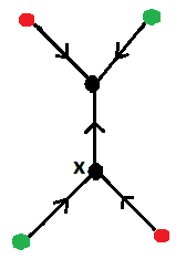
∂(G,fG,OG)=∑x∈VGI∑p=1nx(Gp​x,fGp​x,OGp​x).\partial(G,f_{G},O_{G})=\sum_{x\in V_{G}^{I}}\sum_{p=1}^{n_{x}}(G_{px},f_{G_{px}},O_{G_{px}}).
Refer to caption
Figure 1:

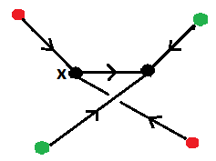
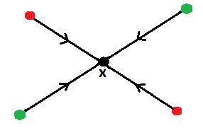
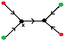
Note that there is no sign in each term of the differential. It is hidden in the way we order the orientation set and orient the new edge. Let us see one example. Assume that r=2r=2, that is, we have 22 colours, and consider the graph in Figure 1. The three graphs that appear in the differential of Figure 1 are Figure 4, Figure 4 and Figure 4.
Refer to caption
Figure 2:
[Uncaptioned image]
Refer to caption
Figure 3:
[Uncaptioned image]
Refer to caption
Figure 4:

To see that for any graph G∈ℰπm1,⋯,mr;dG\in\mathcal{E}_{\pi}^{m_{1},\cdots,m_{r};d}, one has ∂2G=0\partial^{2}G=0, we notice that ∂2G\partial^{2}G is the sum of graphs obtained from GG by inserting two new edges (if we contract these two edges, one should get GG). Each such summand appears in ∂2G\partial^{2}G twice as it matters the order in which the two new edges are created. From the definition of ∂\partial these two repeated summands appear with opposite signs, because in the orientation set

(vp1​x1​ep1​x1)​(vp2​x2​ep2​x2)=−(vp2​x2​ep2​x2)​(vp1​x1​ep1​x1)(v_{p_{1}x_{1}}e_{p_{1}x_{1}})(v_{p_{2}x_{2}}e_{p_{2}x_{2}})=-(v_{p_{2}x_{2}}e_{p_{2}x_{2}})(v_{p_{1}x_{1}}e_{p_{1}x_{1}})

as the degree of (vpi​xi​epi​xi)(v_{p_{i}x_{i}}e_{p_{i}x_{i}}), i=1,2i=1,2, is −d+(d−1)=−1-d+(d-1)=-1.

Now we define ℰHm1,⋯,mr;d\mathcal{E}_{H}^{m_{1},\cdots,m_{r};d} as the cofree cocommutative coalgebra cogenerated by ℰπm1,⋯,mr;d\mathcal{E}_{\pi}^{m_{1},\cdots,m_{r};d}. We can view ℰHm1,⋯,mr;d\mathcal{E}_{H}^{m_{1},\cdots,m_{r};d} as a vector space spanned by all possibly empty or disconnected colored hairy graphs (with each connected component from ℰπm1,⋯,mr;d\mathcal{E}_{\pi}^{m_{1},\cdots,m_{r};d}).

2.2 The rational homotopy of Emb¯c​(∐i=1rℝmi,ℝd)\overline{\mathrm{Emb}}_{c}(\coprod_{i=1}^{r}\mathbb{R}^{m_{i}},\mathbb{R}^{d})

The goal of this subsection is to prove Theorem 0.2, which determines the rational homotopy of the space Emb¯c​(∐i=1rℝmi,ℝd)\overline{\mathrm{Emb}}_{c}(\coprod_{i=1}^{r}\mathbb{R}^{m_{i}},\mathbb{R}^{d}). The plan of the proof is as follows. We will first prove that the graph-complex ℰHm1,⋯,mr;d\mathcal{E}_{H}^{m_{1},\cdots,m_{r};d} is quasi-isomorphic to the complex hRmodΩ(H~∗((∨i=1rSmi)∧⁣∙,ℚ),H^∗(ℬd(∙),ℚ))\underset{\Omega}{\mbox{hRmod}}(\widetilde{H}_{*}((\vee_{i=1}^{r}S^{m_{i}})^{\wedge\bullet},\mathbb{Q}),\widehat{H}_{*}({\mathcal{B}}_{d}(\bullet),\mathbb{Q})) (where ℬd{\mathcal{B}}_{d} denotes the little dd-disks operad). The latter complex is the derived mapping space. Since both the source and target have trivial differential, the complex itself is equivalent to a product of Ext groups that can be either computed by taking the projective resolution of the source (as in Section 4) or by taking the injective resolution of the target. We show that the second approach produces exactly the complex ℰHm1,⋯,mr;d\mathcal{E}_{H}^{m_{1},\cdots,m_{r};d}. A similar argument shows that ℰπm1,⋯,mr;d\mathcal{E}_{\pi}^{m_{1},\cdots,m_{r};d} is equivalent to the derived mapping space hRmodΩ(H~∗((∨i=1rSmi)∧⁣∙,ℚ),ℚ⊗π^∗ℬd(∙))\underset{\Omega}{\mbox{hRmod}}(\widetilde{H}_{*}((\vee_{i=1}^{r}S^{m_{i}})^{\wedge\bullet},\mathbb{Q}),\mathbb{Q}\otimes\widehat{\pi}_{*}{\mathcal{B}}_{d}(\bullet)). On the other hand, since ℰHm1,⋯,mr;d\mathcal{E}_{H}^{m_{1},\cdots,m_{r};d} computes H∗​(Emb¯c​(∐i=1rℝmi,ℝd),ℚ)H_{*}(\overline{\mathrm{Emb}}_{c}(\coprod_{i=1}^{r}\mathbb{R}^{m_{i}},\mathbb{R}^{d}),\mathbb{Q}), by dimensional reasons we conclude that ℰπm1,⋯,mr;d\mathcal{E}_{\pi}^{m_{1},\cdots,m_{r};d} computes ℚ⊗π∗​Emb¯c​(∐i=1rℝmi,ℝd)\mathbb{Q}\otimes\pi_{*}\overline{\mathrm{Emb}}_{c}(\coprod_{i=1}^{r}\mathbb{R}^{m_{i}},\mathbb{R}^{d}). Which finishes the proof of Theorem 0.2.

In [3] Arone and the second author explicitly describe a differential graded right Ω\Omega-modules D^d∙\widehat{D}_{d}^{\bullet} that turns out to be an injective resolution of H^∗​(ℬd​(∙),ℚ)\widehat{H}_{*}({\mathcal{B}}_{d}(\bullet),\mathbb{Q}). We will first recall the right Γ\Gamma-module Dd∙D_{d}^{\bullet}, generated by graphs, introduced in [47]. For k≥0k\geq 0, DdkD_{d}^{k} is a vector space spanned by possibly disconnected graphs with kk external vertices labeled by {1,…,k}\{1,\ldots,k\} of any valence ≥0\geq 0 and some possibly empty set of non-labeled internal vertices of valence ≥3\geq 3, such that each their connected component has at least one external vertex. Tadpoles and multiple edges are allowed. The graphs are oriented, and an orientation set of such graph consists of the union of edges (considered as elements of degree d−1d-1) and internal vertices (considered as elements of degree −d-d). Orienting a graph means putting a total order on its orientation set. As in Section 2.1, there is a similar notion of equivalence of graphs, and similar sign relations. Again as in Section 2.1, the differential is the sum of expansions of vertices. The expansion is applied to both external and internal vertices. The expansion of an internal vertex is as in Section 2.1, while the expansion of an external vertex produces an external vertex (with the same label) and an internal one.

It is well known that the sequence Dd∙={Ddk}k≥0D^{\bullet}_{d}=\{D_{d}^{k}\}_{k\geq 0} is an operad (Figure 5 shows an example of the composition) in differential graded cocommutative coalgebras (Figure 6 is an example of the coproduct in Dd3D_{d}^{3}).

Refer to caption
Figure 5: Examples of the insertion operation
Refer to caption
Figure 6: An example of the coproduct in Dd3D^{3}_{d}

It is also well known [31, 47] that there is an inclusion of operads (in coalgebras) H∗​(ℬd​(∙),ℚ)↪Dd∙H_{*}({\mathcal{B}}_{d}(\bullet),\mathbb{Q})\hookrightarrow D_{d}^{\bullet} that turns out to be a quasi-isomorphism. This inclusion implies that Dd∙D_{d}^{\bullet} is an infinitesimal bimodule over H∗​(ℬd​(∙),ℚ)H_{*}({\mathcal{B}}_{d}(\bullet),\mathbb{Q}), and therefore over H0​(ℬd​(∙),ℚ)=𝒞​o​mH_{0}({\mathcal{B}}_{d}(\bullet),\mathbb{Q})={{\mathcal{C}}om}. By [2, Proposition 4.9], we deduce that Dd∙D_{d}^{\bullet} is a right Γ\Gamma-module. Moreover, since the right Γ\Gamma-module structure respects the coalgebra structure, Dd∙D^{\bullet}_{d} is a right Γ\Gamma-module in coalgebras. Recalling the cross effect functor c​rcr from (1.9), one defines the right Ω\Omega-module D^d∙\widehat{D}_{d}^{\bullet} by

D^d∙=c​r​(Dd∙).\widehat{D}_{d}^{\bullet}=cr(D_{d}^{\bullet}).

It is easy to see (by the definition of the cross effect) that for each k≥0k\geq 0, D^dk\widehat{D}_{d}^{k} is spanned by the same generators as DdkD_{d}^{k}, except that generators of D^dk\widehat{D}_{d}^{k} are graphs whose external vertices are of valence ≥1\geq 1. The following result is [3, Proposition 2.6].

Proposition 2.1.

The right Ω\Omega-module D^d∙\widehat{D}_{d}^{\bullet} is finite dimensional and injective in each homological degree. The inclusion H^∗​(ℬd​(∙),ℚ)↪D^d∙\widehat{H}_{*}({\mathcal{B}}_{d}(\bullet),\mathbb{Q})\hookrightarrow\widehat{D}_{d}^{\bullet} is a quasi-isomorphism of Ω\Omega-modules and thus is an injective resolution for every given complexity.

Remark 2.2.

To recall the decomposition by complexity tt in H^∗​(ℬd​(∙),ℚ)\widehat{H}_{*}({\mathcal{B}}_{d}(\bullet),\mathbb{Q}) is ⨁tH^t⁡(d−1)​(ℬd​(∙),ℚ).\bigoplus_{t}\widehat{H}_{t(d-1)}({\mathcal{B}}_{d}(\bullet),\mathbb{Q}). In D^d∙\widehat{D}_{d}^{\bullet} one defines a similar splitting saying that a complexity of a graph G∈D^dkG\in\widehat{D}_{d}^{k} is the first Betti number of the graph obtained from GG by gluing together all external vertices.

Theorem 2.3.

For d>2​max​{mi| 1≤i≤r}+1d>2\mathrm{max}\{m_{i}|\ 1\leq i\leq r\}+1 the graph-complex ℰHm1,⋯,mr;d\mathcal{E}_{H}^{m_{1},\cdots,m_{r};d} is quasi-isomorphic to hRmodΩ(H~∗((∨i=1rSmi)∧⁣∙,ℚ),H^∗(ℬd(∙),ℚ))\underset{\Omega}{\mathrm{hRmod}}(\widetilde{H}_{*}((\vee_{i=1}^{r}S^{m_{i}})^{\wedge\bullet},\mathbb{Q}),\widehat{H}_{*}({\mathcal{B}}_{d}(\bullet),\mathbb{Q})), that is,

ℰHm1,⋯,mr;d≃hRmodΩ(H~∗((∨i=1rSmi)∧⁣∙,ℚ),H^∗(ℬd(∙),ℚ)).\displaystyle\mathcal{E}_{H}^{m_{1},\cdots,m_{r};d}\simeq\underset{\Omega}{\mathrm{hRmod}}(\widetilde{H}_{*}((\vee_{i=1}^{r}S^{m_{i}})^{\wedge\bullet},\mathbb{Q}),\widehat{H}_{*}({\mathcal{B}}_{d}(\bullet),\mathbb{Q})). (2.1)
Proof.

The steps of the proof are the same as those of the proof of Theorem 2.2 from [3]. Thus, for more details, we refer the reader to [3]. For each k≥0k\geq 0, let M⁡(Ddk)M(D_{d}^{k}) denote the subspace of DdkD_{d}^{k} generated by graphs whose external vertices are of valence =1=1. This space is endowed with a differential being viewed as a quotient-complex of DdkD_{d}^{k}. We have the following quasi-isomorphisms

hRmodΩ(H~∗((∨i=1rSmi)∧⁣∙,ℚ),H^∗(ℬd(∙),ℚ))\displaystyle\underset{\Omega}{\mbox{hRmod}}(\widetilde{H}_{*}((\vee_{i=1}^{r}S^{m_{i}})^{\wedge\bullet},\mathbb{Q}),\widehat{H}_{*}({\mathcal{B}}_{d}(\bullet),\mathbb{Q}))
≃RmodΩ(H~∗((∨i=1rSmi)∧⁣∙,ℚ),D^d∙)byProposition2.1\displaystyle\simeq\ \underset{\Omega}{\mbox{Rmod}}(\widetilde{H}_{*}((\vee_{i=1}^{r}S^{m_{i}})^{\wedge\bullet},\mathbb{Q}),\widehat{D}_{d}^{\bullet})\ \mbox{by}\ \mbox{Proposition}\penalty\ \ref{injective_resolution_prop}
≃⨁k=0∞homΣk(H~∗((∨i=1rSmi)∧k,ℚ),M(Ddk))by[3, Lemma 2.7 and Lemma 2.8]\displaystyle\simeq\bigoplus_{k=0}^{\infty}\mbox{hom}_{\Sigma_{k}}\left(\widetilde{H}_{*}((\vee_{i=1}^{r}S^{m_{i}})^{\wedge k},\mathbb{Q}),M(D_{d}^{k})\right)\ \mbox{by}\ \cite[cite]{[\@@bibref{}{aro_tur13}{}{}, \mbox{Lemma 2.7 and Lemma 2.8}]}
≃⨁k=0∞homΣk(⨁s1+⋯+sr=kIndΣs1×⋯×ΣsrΣkH~∗(Ss1​m1+⋯+sr​mr,ℚ),M(Ddk))by(0.3)\displaystyle\simeq\bigoplus_{k=0}^{\infty}\mbox{hom}_{\Sigma_{k}}\left(\bigoplus_{s_{1}+\cdots+s_{r}=k}\mbox{Ind}^{\Sigma_{k}}_{\Sigma_{s_{1}}\times\cdots\times\Sigma_{s_{r}}}\widetilde{H}_{*}(S^{s_{1}m_{1}+\cdots+s_{r}m_{r}},\mathbb{Q}),M(D_{d}^{k})\right)\ \mbox{by}\ (\ref{homology_wedge})
≃⨁k=0∞⨁s1+⋯+sr=khomΣs1×…×Σsr​(H~∗​(Ss1​m1+⋯+sr​mr,ℚ),M⁡(Ddk)).\displaystyle\simeq\bigoplus_{k=0}^{\infty}\bigoplus_{s_{1}+\cdots+s_{r}=k}\mbox{hom}_{\Sigma_{s_{1}}\times\ldots\times\Sigma_{s_{r}}}\left(\widetilde{H}_{*}(S^{s_{1}m_{1}+\cdots+s_{r}m_{r}},\mathbb{Q}),M(D_{d}^{k})\right).

By the description of the graph-complex ℰHm1,⋯,mr;d\mathcal{E}_{H}^{m_{1},\cdots,m_{r};d} from Section 2.1, it is not difficult to see that there is an isomorphism of chain complexes

ℰHm1,⋯,mr;d≅⨁k=0∞⨁s1+⋯+sr=khomΣs1×…×Σsr​(H~∗​(Ss1​m1+⋯+sr​mr,ℚ),M⁡(Ddk)),\mathcal{E}_{H}^{m_{1},\cdots,m_{r};d}\cong\bigoplus_{k=0}^{\infty}\bigoplus_{s_{1}+\cdots+s_{r}=k}\mbox{hom}_{\Sigma_{s_{1}}\times\ldots\times\Sigma_{s_{r}}}\left(\widetilde{H}_{*}(S^{s_{1}m_{1}+\cdots+s_{r}m_{r}},\mathbb{Q}),M(D_{d}^{k})\right), (2.2)

which completes the proof. ∎

One should mention that the decomposition over (s1,…,sr)(s_{1},\ldots,s_{r}) above appeared exactly as the multidegree Hodge splitting.

Remark 2.4.

A careful reader might prefer to see a product instead of the direct sum used in the above equations. But it is easy to show that ℰHm1,⋯,mr;d\mathcal{E}_{H}^{m_{1},\cdots,m_{r};d} is finite dimensional in every homological degree, for which reason it would not matter whether we take a product or a direct sum of its components, see [2, Remark 13.3] and [3, Section 5] for degree estimates in similar graph-complexes.

The following corollary is an immediate consequence of Theorem 0.1 and Theorem 2.3.

Corollary 2.5.

For d>2​max​{mi| 1≤i≤r}+1d>2\mathrm{max}\{m_{i}|\ 1\leq i\leq r\}+1 the graph-complex ℰHm1,⋯,mr;d\mathcal{E}_{H}^{m_{1},\cdots,m_{r};d} computes the rational homology of the space Emb¯c​(∐i=1rℝmi,ℝd)\overline{\mathrm{Emb}}_{c}(\coprod_{i=1}^{r}\mathbb{R}^{m_{i}},\mathbb{R}^{d}), that is,

H⁡(ℰHm1,⋯,mr;d)≅H∗​(Emb¯c​(∐i=1rℝmi,ℝd),ℚ).\displaystyle H(\mathcal{E}_{H}^{m_{1},\cdots,m_{r};d})\cong H_{*}(\overline{\mathrm{Emb}}_{c}(\coprod_{i=1}^{r}\mathbb{R}^{m_{i}},\mathbb{R}^{d}),\mathbb{Q}). (2.3)
Corollary 2.6.

For d>2​max​{mi| 1≤i≤r}+1d>2\mathrm{max}\{m_{i}|\ 1\leq i\leq r\}+1 the graph-complex ℰπm1,⋯,mr;d\mathcal{E}_{\pi}^{m_{1},\cdots,m_{r};d} computes the rational homotopy of the space Emb¯c​(∐i=1rℝmi,ℝd)\overline{\mathrm{Emb}}_{c}(\coprod_{i=1}^{r}\mathbb{R}^{m_{i}},\mathbb{R}^{d}), that is,

H⁡(ℰπm1,⋯,mr;d)≅ℚ⊗π∗​(Emb¯c​(∐i=1rℝmi,ℝd)).\displaystyle H(\mathcal{E}_{\pi}^{m_{1},\cdots,m_{r};d})\cong\mathbb{Q}\otimes\pi_{*}(\overline{\mathrm{Emb}}_{c}(\coprod_{i=1}^{r}\mathbb{R}^{m_{i}},\mathbb{R}^{d})). (2.4)
Proof.

The desired result is a combination of Corollary 2.5 and the following two facts:

  1. -

    the rational homology of the space Emb¯c​(∐i=1rℝmi,ℝd)\overline{\mathrm{Emb}}_{c}(\coprod_{i=1}^{r}\mathbb{R}^{m_{i}},\mathbb{R}^{d}) is a graded polynomial coalgebra cogenerated by the rational homotopy of the same space;

  2. -

    the subcomplex of ℰHm1,⋯,mr;d\mathcal{E}_{H}^{m_{1},\cdots,m_{r};d}, formed by primitive elements, is exactly the complex ℰπm1,⋯,mr;d\mathcal{E}_{\pi}^{m_{1},\cdots,m_{r};d}.

These two facts imply that (2.3) and (2.4) are equivalent. ∎

Theorem 2.7.

For d>2​max​{mi| 1≤i≤r}+1d>2\mathrm{max}\{m_{i}|\ 1\leq i\leq r\}+1 the graph-complex ℰπm1,⋯,mr;d\mathcal{E}_{\pi}^{m_{1},\cdots,m_{r};d} is quasi-isomorphic to hRmodΩ(H~∗((∨i=1rSmi)∧⁣∙,ℚ),ℚ⊗π^∗ℬd(∙))\underset{\Omega}{\mathrm{hRmod}}(\widetilde{H}_{*}((\vee_{i=1}^{r}S^{m_{i}})^{\wedge\bullet},\mathbb{Q}),\mathbb{Q}\otimes\widehat{\pi}_{*}{\mathcal{B}}_{d}(\bullet)).

Proof.

The proof goes in the same way as that of Theorem 2.3. Instead of D^d∙\widehat{D}_{d}^{\bullet}, one constructs a complex of injective Ω\Omega-modules P^d∙≃ℚ⊗π^∗​ℬd​(∙)\widehat{P}_{d}^{\bullet}\simeq\mathbb{Q}\otimes\widehat{\pi}_{*}{\mathcal{B}}_{d}(\bullet) (see [3, Proposition 2.4] or [47]) defined as the cross effect of the right Γ\Gamma-module Pd∙={Pdk}k≥0P_{d}^{\bullet}=\{P_{d}^{k}\}_{k\geq 0}. Here PdkP_{d}^{k} is the primitive part of DdkD_{d}^{k} – it is spanned by so called internally connected graphs, that have exactly one connected component different from singleton. It is also important that the quasi-isomorphism P^d∙≃ℚ⊗π^∗​ℬd​(∙)\widehat{P}_{d}^{\bullet}\simeq\mathbb{Q}\otimes\widehat{\pi}_{*}{\mathcal{B}}_{d}(\bullet) respects the splitting by complexity tt. In P^d∙⊂D^d∙\widehat{P}_{d}^{\bullet}\subset\widehat{D}_{d}^{\bullet} it is recalled in Remark 2.2, while for the right-hand side it is ℚ⊗π^∗ℬd(∙)≃⊕tℚ⊗π^t⁡(d−2)+1ℬd(∙)\mathbb{Q}\otimes\widehat{\pi}_{*}{\mathcal{B}}_{d}(\bullet)\simeq\oplus_{t}\mathbb{Q}\otimes\widehat{\pi}_{t(d-2)+1}{\mathcal{B}}_{d}(\bullet). ∎

We finally notice that Theorem 0.2 is an immediate consequence of Corollary 2.6 and Theorem 2.7.

2.3 Homotopy graph-complex ℰπm1,⋯,mr;d\mathcal{E}_{\pi}^{m_{1},\cdots,m_{r};d} and the modular envelop of ℒ∞{\mathcal{L}}_{\infty}

Similarly to (2.2), the complex ℰπm1,⋯,mr;d\mathcal{E}_{\pi}^{m_{1},\cdots,m_{r};d} splits into a direct sum of complexes

ℰπm1,⋯,mr;d≅⨁k=1∞⨁s1+⋯+sr=khomΣs1×…×Σsr​(H~∗​(Ss1​m1+⋯+sr​mr,ℚ),M⁡(Pdk)),\mathcal{E}_{\pi}^{m_{1},\cdots,m_{r};d}\cong\bigoplus_{k=1}^{\infty}\bigoplus_{s_{1}+\cdots+s_{r}=k}\mbox{hom}_{\Sigma_{s_{1}}\times\ldots\times\Sigma_{s_{r}}}\left(\widetilde{H}_{*}(S^{s_{1}m_{1}+\cdots+s_{r}m_{r}},\mathbb{Q}),M(P_{d}^{k})\right), (2.5)

where PdkP_{d}^{k} is defined in the proof of Theorem 2.7. Similarly to M⁡(Ddk)M(D_{d}^{k}), one defines M⁡(Pdk)M(P_{d}^{k}) as the quotient complex of PdkP_{d}^{k} spanned by graphs in PdkP_{d}^{k} whose all external vertices are univalent.

The symmetric sequence M⁡(Pd∙)M(P_{d}^{\bullet}) is a sequence of graph-complexes that up to a regrading are components of the modular envelop of ℒ∞{\mathcal{L}}_{\infty}. We briefly recall this connection, while we provide more details in the follow up paper [46].

Cyclic and modular operads were introduced by E. Getzler and M. Kapranov [20, 21]. We will only consider the case when the underlying category is that of chain complexes. In short, a cyclic operad is a usual one O={O⁡(n),n≥0}O=\{O(n),\,n\geq 0\}, for which the output in its elements has the same role as the inputs. In particular O⁡(n)O(n) is acted on by Σn+1\Sigma_{n+1}. To distinguish the cyclic arity with the usual one, one writes O⁡((n))O((n)) for O⁡(n−1)O(n-1). A modular operad is a collection of objects M={M⁡((g,n)),g≥0,n≥0}M=\{M((g,n)),\,g\geq 0,\,n\geq 0\}, such that {M((n))=⊕gM((g,n)),n≥0}\{M((n))=\oplus_{g}M((g,n)),\,n\geq 0\} is a cyclic operad (allowing now cyclic arity 0), and in addition to this structure one also has self-composition maps M⁡((g,n))→M⁡((,,,))M((g,n))\to M((g+1,n-2)), satisfying natural axioms.66 6 For more details, see [21, 28, 35]. Getzler-Kapranov [21] also require the stability condition: M⁡((,,,))=0M((g,n))=0 if 2​g+n−2≤02g+n-2\leq 0, which in particular excludes the unit i​d∈M⁡((,,,))id\in M((0,2)). Following Hinich-Vaintrob [28], we allow M⁡((,,,))M((0,2)) to be one-dimensional spanned by the unit, but require all the other non-stable components to be trivial. If one labels the inputs of M⁡((,,,))M((g_{1},m)) and M⁡((,,,))M((g_{2},n)) by respectively mm and nn elements sets XX and YY, the cyclic compositions are

∘x,y:M((g1,X))⊗M((g2,Y))→M((g1+g2,(X⊔Y)∖{x,y})),x∈X,y∈Y.\circ_{x,y}\colon M((g_{1},X))\otimes M((g_{2},Y))\to M((g_{1}{+}g_{2},(X\sqcup Y)\setminus\{x,y\})),\,\,x\in X,\,y\in Y. (2.6)

The self compositions are

∘x1,x2M((g,X))→M((g+1,X∖{x1,x2})),x1,x2∈X.\circ_{x_{1},x_{2}}M((g,X))\to M((g{+}1,X\setminus\{x_{1},x_{2}\})),\,\,x_{1},x_{2}\in X. (2.7)

One has an adjunction

𝐌𝐨𝐝:CycOp⇄ModOp:𝐂𝐲𝐜\mathbf{Mod}\colon\mathrm{CycOp}\rightleftarrows\mathrm{ModOp}\colon\mathbf{Cyc}

between the categories of cyclic and modular operads [28]. The functor 𝐂𝐲𝐜\mathbf{Cyc} to any modular operad assigns its g=0g=0 part. Its left adjoint 𝐌𝐨𝐝\mathbf{Mod} assigns to a cyclic operad its modular envelop.

As explained by Getzler and Kapranov, the structure of a modular operad admits different twisted versions. One of them associated to the so called cocycle Det\mathrm{Det} is of a special interest as it restricts as the same “non-twisted” cyclic operadic structure. Roughly speaking for this twist, the composition maps (2.6) between different components keep preserving the homological degree, while the self-compositions (2.7) decrease the homological degree by one. One gets a similar adjunction

𝐌𝐨𝐝Det:CycOp⇄ModOpDet:𝐂𝐲𝐜\mathbf{Mod}_{\mathrm{Det}}\colon\mathrm{CycOp}\rightleftarrows\mathrm{ModOp_{\mathrm{Det}}}\colon\mathbf{Cyc}

between the usual cyclic operads and the Det\mathrm{Det}-twisted modular ones.

Proposition 2.8 (Section 3 in [46]).

One has isomorpisms of symmetric sequences in chain complexes

M(P3k)≃ΣkΣk𝐌𝐨𝐝(ℒ∞)((k))⊗signk,k≥1;M(P_{3}^{k})\simeq_{\Sigma_{k}}\Sigma^{k}\mathbf{{Mod}}({\mathcal{L}}_{\infty})((k))\otimes sign_{k},\,\,k\geq 1;
M(P2k)≃ΣkΣ𝐌𝐨𝐝Det(ℒ∞)((k)),k≥1.M(P_{2}^{k})\simeq_{\Sigma_{k}}\Sigma\mathbf{{Mod}}_{\mathrm{Det}}({\mathcal{L}}_{\infty})((k)),\,\,k\geq 1.

Here Σ\Sigma and Σk\Sigma^{k} denote the suspension and kk-iterated suspension, respectively. The genus of the left-hand sides corresponds to the first Betti number of the graphs.77 7 For readers more familiar with the Feynman transform as defined in [21], one has isomorphisms Σ​𝔰​𝐌𝐨𝐝​(ℒ∞)≃FDet​𝒞​o​m\Sigma\mathfrak{s}\mathbf{{Mod}}({\mathcal{L}}_{\infty})\simeq\mathrm{F}_{\mathrm{Det}}{\mathcal{C}}om, Σ​𝔰​𝐌𝐨𝐝Det​(ℒ∞)≃F​𝒞​o​m\Sigma\mathfrak{s}\mathbf{{Mod}}_{\mathrm{Det}}({\mathcal{L}}_{\infty})\simeq\mathrm{F}{\mathcal{C}}om, where Σ\Sigma is the objectwise suspension, and 𝔰\mathfrak{s} is the modular operadic suspension, see [46]. For d>3d>3, the regrading follows from the isomorphism

Mg(Pd+2k)≃ΣkΣ2​(g−1)+2​kMg(Pdk),M_{g}(P_{d+2}^{k})\simeq_{\Sigma_{k}}\Sigma^{2(g-1)+2k}M_{g}(P_{d}^{k}), (2.8)

where MgM_{g} denotes the genus gg part of M⁡(Pd+2k)M(P_{d+2}^{k}) and M⁡(Pdk)M(P_{d}^{k}), respectively .

We conclude the section by recalling the well-known connection to the Vassiliev knot invariants of links [21, Section 5.10], [28]. Consider the complex ℰπm1,⋯,mr;d\mathcal{E}_{\pi}^{m_{1},\cdots,m_{r};d} for m1=…=mr=1m_{1}=\ldots=m_{r}=1, d=3d=3. Thanks to Proposition 2.8 and equation (2.5), we get

ℰπ1,⋯,1;3≅⨁k=1∞⨁s1+⋯+sr=k𝐌𝐨𝐝⁡(ℒ∞)​((k))Σs1×…×Σsr.\mathcal{E}_{\pi}^{1,\cdots,1;3}\cong\bigoplus_{k=1}^{\infty}\bigoplus_{s_{1}+\cdots+s_{r}=k}\mathbf{{Mod}}({\mathcal{L}}_{\infty})((k))_{\Sigma_{s_{1}}\times\ldots\times\Sigma_{s_{r}}}.

The degree zero homology of this complex is expressed in terms of the modular envelop of the Lie operad:

H0​ℰπ1,⋯,1;3≅⨁k=1∞⨁s1+⋯+sr=k𝐌𝐨𝐝⁡(ℒ​i​e)​((k))Σs1×…×Σsr,H_{0}\mathcal{E}_{\pi}^{1,\cdots,1;3}\cong\bigoplus_{k=1}^{\infty}\bigoplus_{s_{1}+\cdots+s_{r}=k}\mathbf{Mod}({\mathcal{L}}ie)((k))_{\Sigma_{s_{1}}\times\ldots\times\Sigma_{s_{r}}},

which is exactly Bar Natan’s space of unitravalent graphs with colored univalent vertices, and which corresponds to the primitive Vassiliev link invariants [4].

3 Low codimensional high dimensional string links

This section is devoted to Conjecture 3.1. We explain here what supports this conjecture and why we think it is true.

Conjecture 3.1.

The statement (2.4) of Corollary 2.6 holds for any codimension d−max⁡{mi| 1≤i≤r}>2d-\mathrm{max}\{m_{i}|\ 1\leq i\leq r\}>2, and any non-negative degree ∗≥0*\geq 0.

There are two things that support this conjecture. Firstly, it is true for r=1r=1, which was recently shown by Fresse, Willwacher, and the second author [19, Remark 19]. Secondly, Theorem 3.2 below shows that it is always true on the level of π0\pi_{0}.

As for the case r=1r=1, we expect two main ingredients in a possible proof of the conjecture: the relative Hopf formality of the little discs operads, which luckily holds in any codimension ≥2\geq 2 [49], and some delooping statement for Emb¯c​(∐i=1rℝmi,ℝd)\overline{\mathrm{Emb}}_{c}(\coprod_{i=1}^{r}\mathbb{R}^{m_{i}},\mathbb{R}^{d}), which would say that Emb¯c​(∐i=1rℝmi,ℝd)\overline{\mathrm{Emb}}_{c}(\coprod_{i=1}^{r}\mathbb{R}^{m_{i}},\mathbb{R}^{d}) is an iterated loop space of the derived mapping space between two algebraic objects described in terms of the little discs operads. Unfortunately, the problem of delooping in the case r≥2r\geq 2 appears to be much more difficult. An attempt for such delooping in the classical case of string links (all mi=1m_{i}=1) has been done in [16]. It describes an interesting possible candidate of the delooping, but unfortunately, the paper has a mistake in the proof of its main result.

Theorem 3.2.

For d−max⁡{mi| 1≤i≤r}>2d-\mathrm{max}\{m_{i}|\ 1\leq i\leq r\}>2, π0​Emb¯c​(∐i=1rℝmi,ℝd)\pi_{0}\overline{\mathrm{Emb}}_{c}(\coprod_{i=1}^{r}\mathbb{R}^{m_{i}},\mathbb{R}^{d}), with the product induced by the concatenation of links, is a finitely generated abelian group. Moreover, one has

ℚ⊗π0​Emb¯c​(∐i=1rℝmi,ℝd)≃H0​ℰπm1,⋯,mr;d.\displaystyle\mathbb{Q}\otimes\pi_{0}\overline{\mathrm{Emb}}_{c}(\coprod_{i=1}^{r}\mathbb{R}^{m_{i}},\mathbb{R}^{d})\simeq H_{0}\mathcal{E}_{\pi}^{m_{1},\cdots,m_{r};d}. (3.1)

One should mention that the fact that πi​Emb¯c​(∐i=1rℝmi,ℝd)\pi_{i}\overline{\mathrm{Emb}}_{c}(\coprod_{i=1}^{r}\mathbb{R}^{m_{i}},\mathbb{R}^{d}), i>0i>0, are finitely generated abelian groups, easily follows from the embedding calculus, which is always applicable when codimension >2>2 [22, 23].

This theorem is a consequence of Lemmas 3.3 and 3.8. Let us first understand the right-hand side of (3.1). The complex ℰπm1,⋯,mr;d\mathcal{E}_{\pi}^{m_{1},\cdots,m_{r};d} splits into a direct sum of complexes

ℰπm1,⋯,mr;d=⨁g≥0ℰg​πm1,⋯,mr;d,\mathcal{E}_{\pi}^{m_{1},\cdots,m_{r};d}=\bigoplus_{g\geq 0}\mathcal{E}_{g\pi}^{m_{1},\cdots,m_{r};d},

where ℰg​πm1,⋯,mr;d\mathcal{E}_{g\pi}^{m_{1},\cdots,m_{r};d} is spanned by the graphs whose first Betti number (== genus) is gg.

Lemma 3.3.

For d−max⁡{mi| 1≤i≤r}>2d-\mathrm{max}\{m_{i}|\ 1\leq i\leq r\}>2, H≤0​ℰπm1,⋯,mr;d=H≤0​ℰ0​πm1,⋯,mr;dH_{\leq 0}\mathcal{E}_{\pi}^{m_{1},\cdots,m_{r};d}=H_{\leq 0}\mathcal{E}_{0\pi}^{m_{1},\cdots,m_{r};d}.

Proof.

It is enough to show that all the graphs of positive genus have positive homological degree. One can proceed by induction. The degree of any graph of the form is d−mi−2>0d-m_{i}-2>0. Any uni-trivalent hairy graph is obtained from by a sequence of attachments of hairs (inside an edge) and edges (both endpoints on the same edge or on two different ones). The first operation creates 2 new edges and two vertices – one external and one internal. The total degree change is

2​(d−1)−d−mi=d−mi−2>0.2(d-1)-d-m_{i}=d-m_{i}-2>0.

The second operation creates 3 new edges and two new internal vertices. The total degree change is

3​(d−1)−2​d=d−3>0.3(d-1)-2d=d-3>0.

Finally, any other hairy graph is obtained from a uni-trivalent one by a seqence of contractions of edges. Each such contraction increases the degree by one. ∎

In case r=1r=1, H∗​ℰ0​πm1,dH_{*}\mathcal{E}_{0\pi}^{m_{1},d} is always one-dimensional. In case of even codimension d−m1d-m_{1}, it is spanned by the line graph of degree d−2​m1−1d-2m_{1}-1; in case of odd codimension – by the tripod of degree 2​d−2​m1−32d-2m_{1}-3. The following result was obtained in [19, Corollary 20] as a corollary of (3.1), which was proved there for r=1r=1.

Corollary 3.4 ([19]).

For d−m>2d-m>2, π0​Emb¯c​(ℝm,ℝd)\pi_{0}\overline{\mbox{Emb}}_{c}(\mathbb{R}^{m},\mathbb{R}^{d}) is a finitely generated abelian group of rank ≤1\leq 1. It is infinite only if either m=2​k+1m=2k+1, d=4​k+3d=4k+3, k≥1k\geq 1, or m=4​k−1m=4k-1, d=6​kd=6k, k≥1k\geq 1.

One has a fiber sequence

Emb¯c​(ℝm,ℝd)→Embc​(ℝm,ℝd)→Ωm​Vm​(ℝd),\displaystyle\overline{\mbox{Emb}}_{c}(\mathbb{R}^{m},\mathbb{R}^{d})\to\mbox{Emb}_{c}(\mathbb{R}^{m},\mathbb{R}^{d})\to\Omega^{m}V_{m}(\mathbb{R}^{d}), (3.2)

where Vm​(ℝd)V_{m}(\mathbb{R}^{d}) is the Stiefel manifold S​O​(d)/S​O​(d−m)SO(d)/SO(d-m). (By the Smale-Hirsch principle Immc​(ℝm,ℝd)≃Ωm​Vm​(ℝd)\mbox{Imm}_{c}(\mathbb{R}^{m},\mathbb{R}^{d})\simeq\Omega^{m}V_{m}(\mathbb{R}^{d})). From (3.2) we get the long exact sequence

…→πm+1​Vm​(ℝd)⟶j∗π0​Emb¯c​(ℝm,ℝd)⟶k∗π0​Embc​(ℝm,ℝd)⟶l∗πm​Vm​(ℝd).\displaystyle\ldots\to\pi_{m+1}V_{m}(\mathbb{R}^{d})\stackrel{{\scriptstyle j_{*}}}{{\longrightarrow}}\pi_{0}\overline{\mathrm{Emb}}_{c}(\mathbb{R}^{m},\mathbb{R}^{d})\stackrel{{\scriptstyle k_{*}}}{{\longrightarrow}}\pi_{0}\mathrm{Emb}_{c}(\mathbb{R}^{m},\mathbb{R}^{d})\stackrel{{\scriptstyle l_{*}}}{{\longrightarrow}}\pi_{m}V_{m}(\mathbb{R}^{d}). (3.3)

The case m=2​k+1m=2k+1, d=4​k+3d=4k+3, k≥1k\geq 1, of the corollary corresponds to the graph-cycle . Geometrically it appears as the image under j∗j_{*} of the Euler class of S​O​(d−m)SO(d-m) in Vm​(ℝd)=S​O​(d)/S​O​(d−m)V_{m}(\mathbb{R}^{d})=SO(d)/SO(d-m). The case m=4​k−1m=4k-1, d=6​kd=6k, k≥1k\geq 1, corresponds to the graph-cycle . Its image in π0​Embc​(ℝm,ℝd)\pi_{0}\mathrm{Emb}_{c}(\mathbb{R}^{m},\mathbb{R}^{d}) under k∗k_{*} is the Haefliger trefoil [26], which is known to be trivial as immersion (equivalently lies in the image of k∗k_{*}).

To describe H0​ℰ0​πm1,⋯,mr;dH_{0}\mathcal{E}_{0\pi}^{m_{1},\cdots,m_{r};d} we recall some standard facts and notation.

The operad ℒ​i​e{{\mathcal{L}}ie} is cyclic, thus ℒ​i​e​(n−1)=ℒ​i​e​((n)){{\mathcal{L}}ie}(n-1)={{\mathcal{L}}ie}((n)) is a Σn\Sigma_{n}-module. The following result is well known.

Lemma 3.5 ([32, 25, 12]).

For n≥1n\geq 1, one has

ℒie((n))≃Σnker(IndΣn−1Σnℒie(n−1)→qℒie(n)),{{\mathcal{L}}ie}((n))\simeq_{\Sigma_{n}}\mathrm{ker}\left(\mathrm{Ind}^{\Sigma_{n}}_{\Sigma_{n-1}}{{\mathcal{L}}ie}(n-1)\stackrel{{\scriptstyle q}}{{\to}}{{\mathcal{L}}ie}(n)\right),

where the map qq is described below.

Elements of IndΣn−1Σn​ℒ​i​e​(n−1)\mathrm{Ind}^{\Sigma_{n}}_{\Sigma_{n-1}}{{\mathcal{L}}ie}(n-1) can be written in the form ∑i=1nαi​xi⊗fi​(x1,…,x^i,…,xn)\sum_{i=1}^{n}\alpha_{i}x_{i}\otimes f_{i}(x_{1},\ldots,\widehat{x}_{i},\ldots,x_{n}), where αi∈ℚ\alpha_{i}\in\mathbb{Q}, fi∈ℒ​i​e​(n−1)f_{i}\in{{\mathcal{L}}ie}(n-1). The map qq sends

q:xi⊗fi​(x1,…,x^i,…,xn)↦[xi,fi​(x1,…,x^i,…,xn)].q\colon x_{i}\otimes f_{i}(x_{1},\ldots,\widehat{x}_{i},\ldots,x_{n})\mapsto[x_{i},f_{i}(x_{1},\ldots,\widehat{x}_{i},\ldots,x_{n})].

For any symmetric sequence M⁡(∙)M(\bullet) and any graded vector space VV, we denote by

FM⁡(∙)​(V):=⨁k≥0M⁡(k)⊗ΣkV⊗k.F_{M(\bullet)}(V):=\bigoplus_{k\geq 0}M(k)\otimes_{\Sigma_{k}}V^{\otimes k}.
Lemma 3.6.

For any d−max⁡{mi| 1≤i≤r}>2d-\mathrm{max}\{m_{i}|\ 1\leq i\leq r\}>2,

H∗ℰ0​πm1,⋯,mr;d=Σ−d+3Fℒ​i​e​((∙))(H~∗(∨i=1rSd−mi−2,ℚ)).H_{*}\mathcal{E}_{0\pi}^{m_{1},\cdots,m_{r};d}=\Sigma^{-d+3}F_{{{\mathcal{L}}ie}((\bullet))}(\tilde{H}_{*}(\vee_{i=1}^{r}S^{d-m_{i}-2},\mathbb{Q})).
Proof.

It is well known that the homology of the complex of trees, whose leaves are bijectively labeled by {1,…,n}\{1,\ldots,n\}, is concentrated in the top homological degree and (up to a regrading and a possible tensor with the sign representation) is isomorphic to ℒ​i​e​((n)){{\mathcal{L}}ie}((n)), see [54]. This also follows from Proposition 2.8 and equation (2.8) applied for g=0g=0. A careful count of the degrees and signs finishes the proof. ∎

In particular, this lemma says that H0​ℰ0​πm1,⋯,mr;dH_{0}\mathcal{E}_{0\pi}^{m_{1},\cdots,m_{r};d} is isomorphic to the degree d−3d-3 part of Fℒ​i​e​((∙))(H~∗(∨i=1rSd−mi−2,ℚ))F_{{{\mathcal{L}}ie}((\bullet))}(\tilde{H}_{*}(\vee_{i=1}^{r}S^{d-m_{i}-2},\mathbb{Q})).

Now we want to concentrate on the left-hand side of (3.1). Let Emb⁡(∐i=1rSmi,Sd)\mathrm{Emb}(\coprod_{i=1}^{r}S^{m_{i}},S^{d}) be the space of smooth spherical links ∐i=1rSmi↪Sd\coprod_{i=1}^{r}S^{m_{i}}\hookrightarrow S^{d}. It was shown by A. Haefliger [27] that for d−max⁡{mi| 1≤i≤r}>2d-\mathrm{max}\{m_{i}|\ 1\leq i\leq r\}>2, π0​Emb​(∐i=1rSmi,Sd)\pi_{0}\mathrm{Emb}(\coprod_{i=1}^{r}S^{m_{i}},S^{d}) is a finitely generated abelian group, whose product is defined as follows. Given two links L1,L2∈Emb⁡(∐i=1rSmi,Sd)L_{1},L_{2}\in\mathrm{Emb}(\coprod_{i=1}^{r}S^{m_{i}},S^{d}), we move one inside one semisphere, and the other inside the complement semisphere. Then we connect the components of L1L_{1} with the corresponding components of L2L_{2} by very narrow tubes to form a new link. The result as an element of π0​Emb​(∐i=1rSmi,Sd)\pi_{0}\mathrm{Emb}(\coprod_{i=1}^{r}S^{m_{i}},S^{d}) does not depend on the paths of the tubes since the complement of L1​∐L2L_{1}\coprod L_{2} is simply connected. By π0U​Emb​(∐i=1rSmi,Sd)\pi_{0}^{U}\mathrm{Emb}(\coprod_{i=1}^{r}S^{m_{i}},S^{d}), π0U​Embc​(∐i=1rℝmi,ℝd)\pi_{0}^{U}\mathrm{Emb}_{c}(\coprod_{i=1}^{r}\mathbb{R}^{m_{i}},\mathbb{R}^{d}), π0U​Emb¯c​(∐i=1rℝmi,ℝd)\pi_{0}^{U}\overline{\mathrm{Emb}}_{c}(\coprod_{i=1}^{r}\mathbb{R}^{m_{i}},\mathbb{R}^{d}) we denote the kernel of the corresponding map

π0​Emb​(∐i=1rSmi,Sd)→∏i=1rπ0​Emb​(Smi,Sd);\displaystyle\pi_{0}\mathrm{Emb}(\coprod_{i=1}^{r}S^{m_{i}},S^{d})\to\prod_{i=1}^{r}\pi_{0}\mathrm{Emb}(S^{m_{i}},S^{d});
π0​Embc​(∐i=1rℝmi,ℝd)→∏i=1rπ0​Embc​(ℝmi,ℝd);\displaystyle\pi_{0}\mathrm{Emb}_{c}(\coprod_{i=1}^{r}\mathbb{R}^{m_{i}},\mathbb{R}^{d})\to\prod_{i=1}^{r}\pi_{0}\mathrm{Emb}_{c}(\mathbb{R}^{m_{i}},\mathbb{R}^{d});
π0​Emb¯c​(∐i=1rℝmi,ℝd)→∏i=1rπ0​Emb¯c​(ℝmi,ℝd).\displaystyle\pi_{0}\overline{\mathrm{Emb}}_{c}(\coprod_{i=1}^{r}\mathbb{R}^{m_{i}},\mathbb{R}^{d})\to\prod_{i=1}^{r}\pi_{0}\overline{\mathrm{Emb}}_{c}(\mathbb{R}^{m_{i}},\mathbb{R}^{d}).

The letter UU refers to “unknot”. Each of the groups is the subgroup of links formed by unknots.

The following lemma proves the first statement of Theorem 3.2. Its proof is an easy exercise, which we leave to the reader.

Lemma 3.7.

For d−max⁡{mi| 1≤i≤r}>2d-\mathrm{max}\{m_{i}|\ 1\leq i\leq r\}>2, one has isomorphisms of monoids (and thus of finitely generated abelian groups):

  • •

    π0​Embc​(∐i=1rℝmi,ℝd)≃π0​Emb​(∐i=1rSmi,Sd)\pi_{0}\mathrm{Emb}_{c}(\coprod_{i=1}^{r}\mathbb{R}^{m_{i}},\mathbb{R}^{d})\simeq\pi_{0}\mathrm{Emb}(\coprod_{i=1}^{r}S^{m_{i}},S^{d});

  • •

    π0U​Emb¯c​(∐i=1rℝmi,ℝd)≃π0U​Embc​(∐i=1rℝmi,ℝd)≃π0U​Emb​(∐i=1rSmi,Sd)\pi_{0}^{U}\overline{\mathrm{Emb}}_{c}(\coprod_{i=1}^{r}\mathbb{R}^{m_{i}},\mathbb{R}^{d})\simeq\pi_{0}^{U}\mathrm{Emb}_{c}(\coprod_{i=1}^{r}\mathbb{R}^{m_{i}},\mathbb{R}^{d})\simeq\pi_{0}^{U}\mathrm{Emb}(\coprod_{i=1}^{r}S^{m_{i}},S^{d});

  • •

    π0​Emb¯c​(∐i=1rℝmi,ℝd)≃π0U​Emb¯c​(∐i=1rℝmi,ℝd)×∏i=1rπ0​Emb¯c​(ℝmi,ℝd)\pi_{0}\overline{\mathrm{Emb}}_{c}(\coprod_{i=1}^{r}\mathbb{R}^{m_{i}},\mathbb{R}^{d})\simeq\pi_{0}^{U}\overline{\mathrm{Emb}}_{c}(\coprod_{i=1}^{r}\mathbb{R}^{m_{i}},\mathbb{R}^{d})\times\prod_{i=1}^{r}\pi_{0}\overline{\mathrm{Emb}}_{c}(\mathbb{R}^{m_{i}},\mathbb{R}^{d}).

By [27] and Corollary 3.4, π0​Emb​(∐i=1rSmi,Sd)\pi_{0}\mathrm{Emb}(\coprod_{i=1}^{r}S^{m_{i}},S^{d}) and π0​Emb¯c​(ℝmi,ℝd)\pi_{0}\overline{\mathrm{Emb}}_{c}(\mathbb{R}^{m_{i}},\mathbb{R}^{d}) are finitely generated abelian groups, thus π0​Emb¯c​(∐i=1rℝmi,ℝd)\pi_{0}\overline{\mathrm{Emb}}_{c}(\coprod_{i=1}^{r}\mathbb{R}^{m_{i}},\mathbb{R}^{d}) is so as well.

Define the groups

Π¯m1​…​mr​d:=πd−2(∨i=1rSd−mi−1);\displaystyle\overline{\Pi}^{m_{1}\ldots m_{r}d}:=\pi_{d-2}(\vee_{i=1}^{r}S^{d-m_{i}-1});
Λ¯m1​…​mr​d:=⨁i=1rπmi(∨i=1rSd−mi−1);\displaystyle\overline{\Lambda}^{m_{1}\ldots m_{r}d}:=\bigoplus_{i=1}^{r}\pi_{m_{i}}(\vee_{i=1}^{r}S^{d-m_{i}-1});
K¯m1​…​mr​d:=ker⁡(Λ¯m1​…​mr​d⟶q0Π¯m1​…​mr​d),\displaystyle\overline{K}^{m_{1}\ldots m_{r}d}:=\mathrm{ker}(\overline{\Lambda}^{m_{1}\ldots m_{r}d}\stackrel{{\scriptstyle q_{0}}}{{\longrightarrow}}\overline{\Pi}^{m_{1}\ldots m_{r}d}),

here q0:(α1​…​αr)↦∑i=1r[ιi,αi]q_{0}\colon(\alpha_{1}\ldots\alpha_{r})\mapsto\sum_{i=1}^{r}[\iota_{i},\alpha_{i}], where [.,.][\,.\,,\,.\,] is the Whitehead bracket, ιi∈πd−mi−1(∨i=1rSd−mi−1)\iota_{i}\in\pi_{d-m_{i}-1}(\vee_{i=1}^{r}S^{d-m_{i}-1}) is the element encoding the inclusion of the ii-th summand Sd−mi−1↪∨i=1rSd−mi−1S^{d-m_{i}-1}\hookrightarrow\vee_{i=1}^{r}S^{d-m_{i}-1}. We also define their subgroups

Πm1​…​mr​d:=ker(πd−2(∨i=1rSd−mi−1)→⨁i=1rπd−2Sd−mi−1);\displaystyle\Pi^{m_{1}\ldots m_{r}d}:=\mathrm{ker}\left(\pi_{d-2}(\vee_{i=1}^{r}S^{d-m_{i}-1})\to\bigoplus_{i=1}^{r}\pi_{d-2}S^{d-m_{i}-1}\right);
Λm1​…​mr​d:=⨁i=1rker(πmi(∨i=1rSd−mi−1)→πmiSd−mi−1);\displaystyle\Lambda^{m_{1}\ldots m_{r}d}:=\bigoplus_{i=1}^{r}\mathrm{ker}\left(\pi_{m_{i}}(\vee_{i=1}^{r}S^{d-m_{i}-1})\to\pi_{m_{i}}S^{d-m_{i}-1}\right);
Km1​…​mr​d:=ker⁡(Λm1​…​mr​d⟶q0|ΛΠm1​…​mr​d).\displaystyle K^{m_{1}\ldots m_{r}d}:=\mathrm{ker}(\Lambda^{m_{1}\ldots m_{r}d}\stackrel{{\scriptstyle q_{0}|_{\Lambda}}}{{\longrightarrow}}\Pi^{m_{1}\ldots m_{r}d}).
Lemma 3.8.

For d−max⁡{mi| 1≤i≤r}>2d-\mathrm{max}\{m_{i}|\ 1\leq i\leq r\}>2,

ℚ⊗π0​Emb¯c​(∐i=1rℝmi,ℝd)≃ℚ⊗K¯m1​…​mr​d≃H0​ℰ0​πm1,⋯,mr;d.\displaystyle\mathbb{Q}\otimes\pi_{0}\overline{\mathrm{Emb}}_{c}(\coprod_{i=1}^{r}\mathbb{R}^{m_{i}},\mathbb{R}^{d})\simeq\mathbb{Q}\otimes\overline{K}^{m_{1}\ldots m_{r}d}\simeq H_{0}\mathcal{E}_{0\pi}^{m_{1},\cdots,m_{r};d}. (3.4)
Proof.

We prove below the second isomorphism in (3.4) for any r≥1r\geq 1. Thus, by Corollary 3.4 it’s enough to show the first isomorphism only for r≥2r\geq 2. In [27], A. Haefliger develops a homotopical approach to compute π0​Emb​(∐i=1rSmi,Sd)\pi_{0}\mathrm{Emb}(\coprod_{i=1}^{r}S^{m_{i}},S^{d}). Using this method it was shown in [13, Lemma 1.3] that

ℚ⊗π0U​Emb​(∐i=1rSmi,Sd)=ℚ⊗Km1​…​mr​d.\mathbb{Q}\otimes\pi_{0}^{U}\mathrm{Emb}(\coprod_{i=1}^{r}S^{m_{i}},S^{d})=\mathbb{Q}\otimes K^{m_{1}\ldots m_{r}d}.

Applying Lemma 3.7, we get

ℚ⊗π0​Emb¯c​(∐i=1rℝmi,ℝd)≃ℚ⊗π0U​Emb¯c​(∐i=1rℝmi,ℝd)⊕⨁i=1rℚ⊗π0​Emb¯c​(ℝmi,ℝd)≃ℚ⊗Km1​…​mr​d⊕⨁i=1rℚ⊗K¯mi​d≃ℚ⊗K¯m1​…​mr​d.\mathbb{Q}\otimes\pi_{0}\overline{\mathrm{Emb}}_{c}(\coprod_{i=1}^{r}\mathbb{R}^{m_{i}},\mathbb{R}^{d})\simeq\mathbb{Q}\otimes\pi_{0}^{U}\overline{\mathrm{Emb}}_{c}(\coprod_{i=1}^{r}\mathbb{R}^{m_{i}},\mathbb{R}^{d})\oplus\bigoplus_{i=1}^{r}\mathbb{Q}\otimes\pi_{0}\overline{\mathrm{Emb}}_{c}(\mathbb{R}^{m_{i}},\mathbb{R}^{d})\\ \simeq\mathbb{Q}\otimes K^{m_{1}\ldots m_{r}d}\oplus\bigoplus_{i=1}^{r}\mathbb{Q}\otimes\overline{K}^{m_{i}d}\simeq\mathbb{Q}\otimes\overline{K}^{m_{1}\ldots m_{r}d}.

The last isomorphism is due to the splittings

Π¯m1​…​mr​d=Πm1​…​mr​d⊕⨁i=1rπd−2​Sd−mi−1=Πm1​…​mr​d⊕⨁i=1rΠ¯mi​d;\displaystyle\overline{\Pi}^{m_{1}\ldots m_{r}d}=\Pi^{m_{1}\ldots m_{r}d}\oplus\bigoplus_{i=1}^{r}\pi_{d-2}S^{d-m_{i}-1}=\Pi^{m_{1}\ldots m_{r}d}\oplus\bigoplus_{i=1}^{r}\overline{\Pi}^{m_{i}d};
Λ¯m1​…​mr​d=Λm1​…​mr​d⊕⨁i=1rπmi​Sd−mi−1=Λm1​…​mr​d⊕⨁i=1rΛ¯mi​d,\displaystyle\overline{\Lambda}^{m_{1}\ldots m_{r}d}=\Lambda^{m_{1}\ldots m_{r}d}\oplus\bigoplus_{i=1}^{r}\pi_{m_{i}}S^{d-m_{i}-1}=\Lambda^{m_{1}\ldots m_{r}d}\oplus\bigoplus_{i=1}^{r}\overline{\Lambda}^{m_{i}d},

and also the fact that q0q_{0} sends each summand of Λ¯m1​…​mr​d\overline{\Lambda}^{m_{1}\ldots m_{r}d} to the corresponding summand of Π¯m1​…​mr​d\overline{\Pi}^{m_{1}\ldots m_{r}d}.

To see the second isomorphism of (3.4), we notice that

ℚ⊗π∗(∨i=1rSd−mi−1)≃ΣFℒ​i​e​(∙)(H~∗(∨i=1rSd−mi−2,ℚ)).\mathbb{Q}\otimes\pi_{*}(\vee_{i=1}^{r}S^{d-m_{i}-1})\simeq\Sigma F_{{{\mathcal{L}}ie}(\bullet)}(\tilde{H}_{*}(\vee_{i=1}^{r}S^{d-m_{i}-2},\mathbb{Q})).

Thus ℚ⊗Π¯m1​…​mr​d\mathbb{Q}\otimes\overline{\Pi}^{m_{1}\ldots m_{r}d} is the degree d−3d-3 part of Fℒ​i​e​(∙)(H~∗(∨i=1rSd−mi−2,ℚ))F_{{{\mathcal{L}}ie}(\bullet)}(\tilde{H}_{*}(\vee_{i=1}^{r}S^{d-m_{i}-2},\mathbb{Q})). Similarly, one can see that ℚ⊗Λ¯m1​…​mr​d\mathbb{Q}\otimes\overline{\Lambda}^{m_{1}\ldots m_{r}d} is the degree d−3d-3 part of FIndΣ∙Σ∙−1ℒie(∙−1)(H~∗(∨i=1rSd−mi−2,ℚ))F_{\mathrm{Ind}^{\Sigma_{\bullet}}_{\Sigma_{\bullet-1}}{{\mathcal{L}}ie}(\bullet-1)}(\tilde{H}_{*}(\vee_{i=1}^{r}S^{d-m_{i}-2},\mathbb{Q})). Thus K¯m1​…​mr​d\overline{K}^{m_{1}\ldots m_{r}d} is the degree d−3d-3 part of

ker(FIndΣ∙Σ∙−1ℒie(∙−1)(H~∗(∨i=1rSd−mi−2,ℚ))⟶FqFℒ​i​e​(∙)(H~∗(∨i=1rSd−mi−2,ℚ))),\mathrm{ker}\left(F_{\mathrm{Ind}^{\Sigma_{\bullet}}_{\Sigma_{\bullet-1}}{{\mathcal{L}}ie}(\bullet-1)}(\tilde{H}_{*}(\vee_{i=1}^{r}S^{d-m_{i}-2},\mathbb{Q}))\stackrel{{\scriptstyle F_{q}}}{{\longrightarrow}}F_{{{\mathcal{L}}ie}(\bullet)}(\tilde{H}_{*}(\vee_{i=1}^{r}S^{d-m_{i}-2},\mathbb{Q}))\right),

which by Lemmas 3.5 and 3.6 is the same as H0​ℰ0​πm1,⋯,mr;dH_{0}\mathcal{E}_{0\pi}^{m_{1},\cdots,m_{r};d}.

∎

4 The Koszul complexes

By Theorems 0.1 and 0.2, the rational homology and homotopy of Emb¯c​(∐i=1rℝmi,ℝd)\overline{\mathrm{Emb}}_{c}(\coprod_{i=1}^{r}\mathbb{R}^{m_{i}},\mathbb{R}^{d}) is described in terms of derived maps of right Ω\Omega-modules. In this section we exhibit explicit complexes computing the (co)homology and homotopy of Emb¯c​(∐i=1rℝmi,ℝd)\overline{\mathrm{Emb}}_{c}(\coprod_{i=1}^{r}\mathbb{R}^{m_{i}},\mathbb{R}^{d}) by considering the projective resolution of the source Ω\Omega-modules in (0.10) and (0.11). We call these complexes Koszul as they are constructed using operadic language and the Koszul duality between the commutative and Lie operads. At the end of the section we show that the Koszul complexes can also be used to understand rationally the stages of the Goodwillie-Weiss towers for Emb¯c​(∐i=1rℝmi,ℝd)\overline{\mathrm{Emb}}_{c}(\coprod_{i=1}^{r}\mathbb{R}^{m_{i}},\mathbb{R}^{d}).

For s1,⋯,sr≥0s_{1},\cdots,s_{r}\geq 0, recall the definition of the right Ω\Omega-module Qs1⋯srm1⋯mrQ_{s_{1}\cdots s_{r}}^{m_{1}\cdots m_{r}} (it was introduced in (0)).

Qs1⋯srm1⋯mr(k)={0ifk≠s1+⋯+srIndΣkΣs1×⋯×ΣsrH~∗(Ss1​m1+⋯+sr​mr;ℚ)ifk=s1+⋯+sr\displaystyle Q_{s_{1}\cdots s_{r}}^{m_{1}\cdots m_{r}}(k)=\left\{\begin{array}[]{lll}0&\mbox{if}&k\neq s_{1}+\cdots+s_{r}\\ \mbox{Ind}^{\Sigma_{k}}_{\Sigma_{s_{1}}\times\cdots\times\Sigma_{s_{r}}}\widetilde{H}_{*}(S^{s_{1}m_{1}+\cdots+s_{r}m_{r}};\mathbb{Q})&\mbox{if}&k=s_{1}+\cdots+s_{r}\end{array}\right.
Proposition 4.1.

For d>2​max​{mi| 1≤i≤r}+1d>2\mathrm{max}\{m_{i}|\ 1\leq i\leq r\}+1, one has quasi-isomorphisms

C∗(Emb¯c(∐i=1rℝmi,ℝd),⊗ℚ)≃⨁s1,⋯,sr,t≥0hRmodΩ(Qs1⋯srm1⋯mr,H^t⁡(d−1)(C(∙,ℝd);ℚ))\displaystyle C_{*}(\overline{\mathrm{Emb}}_{c}(\coprod_{i=1}^{r}\mathbb{R}^{m_{i}},\mathbb{R}^{d}),\otimes\mathbb{Q})\simeq\bigoplus_{s_{1},\cdots,s_{r},t\geq 0}\underset{\Omega}{\mathrm{hRmod}}(Q^{m_{1}\cdots m_{r}}_{s_{1}\cdots s_{r}},\widehat{H}_{t(d-1)}(C(\bullet,\mathbb{R}^{d});\mathbb{Q})) (4.4)
π∗Emb¯c(∐i=1rℝmi,ℝd)⊗ℚ≃⨁s1,⋯,sr,t≥0hRmodΩ(Qs1⋯srm1⋯mr,π^t⁡(d−2)+1C(∙,ℝd)⊗ℚ)\displaystyle\ \pi_{*}\overline{\mathrm{Emb}}_{c}(\coprod_{i=1}^{r}\mathbb{R}^{m_{i}},\mathbb{R}^{d})\otimes\mathbb{Q}\simeq\bigoplus_{s_{1},\cdots,s_{r},t\geq 0}\underset{\Omega}{\mathrm{hRmod}}(Q^{m_{1}\cdots m_{r}}_{s_{1}\cdots s_{r}},\widehat{\pi}_{t(d-2)+1}C(\bullet,\mathbb{R}^{d})\otimes\mathbb{Q}) (4.5)
Proof.

This is a direct consequence of Theorems 0.1 and 0.2 and the fact that both the source and target Ω\Omega-modules in (0.1) and 0.2 split into a direct sum/product. The only thing we need to understand is why the product can be replaced by the direct sum. This follows for example, from Remark 2.4. ∎

4.1 The Koszul resolution and Koszul dual of Qs1⋯srm1⋯mrQ_{s_{1}\cdots s_{r}}^{m_{1}\cdots m_{r}}

In this section we will find a cofibrant replacement (the model structure we use in the category RmodΩ\underset{\Omega}{\mbox{Rmod}} is the one whose weak equivalences and fibrations are levelwise), denoted by CQm1⋯mrs1⋯srCQ^{m_{1}\cdots m_{r}}_{s_{1}\cdots s_{r}}, of Qm1⋯mrs1⋯srQ^{m_{1}\cdots m_{r}}_{s_{1}\cdots s_{r}}. We cal this cofibrant replacement Koszul resolution of Qm1⋯mrs1⋯srQ^{m_{1}\cdots m_{r}}_{s_{1}\cdots s_{r}}. The idea of this construction is to use the fact that the right Ω\Omega-module structure is the same as the right module structure over the commutative non-unital operad 𝒞​o​m+{\mathcal{C}}om_{+} and then use the Koszul duality between the commutative and Lie operads. We will follow exactly the same steps as in [3, Section 5 and Section 6], where this was done for r=1r=1. As an Ω\Omega-module, CQm1⋯mrs1⋯srCQ^{m_{1}\cdots m_{r}}_{s_{1}\cdots s_{r}} is freely generated by a symmetric sequence that we denote by KQm1⋯mrs1⋯srKQ^{m_{1}\cdots m_{r}}_{s_{1}\cdots s_{r}} and we call it Koszul dual of Qm1⋯mrs1⋯srQ^{m_{1}\cdots m_{r}}_{s_{1}\cdots s_{r}}.88 8 One should not confuse the terms Koszul complexes, which are complexes computing the (co)homology or homotopy of embedding spaces, Koszul resolutions, which refer to a cofibrant replacement of Ω\Omega-modules, and Koszul duals which refer to symmetric sequences (in fact to right c​o​ℒ​i​e​[1]co{\mathcal{L}}ie[1]-comodules). We will also explicitly describe CQm1⋯mrs1⋯srCQ^{m_{1}\cdots m_{r}}_{s_{1}\cdots s_{r}} (and then explicitly describe KQm1⋯mrs1⋯srKQ^{m_{1}\cdots m_{r}}_{s_{1}\cdots s_{r}}) in terms of spaces of colored forests.

Let us start with an explicit description of CQm1⋯mrs1⋯srCQ^{m_{1}\cdots m_{r}}_{s_{1}\cdots s_{r}}. For r=1r=1, Qm1⋯mrs1⋯srQ^{m_{1}\cdots m_{r}}_{s_{1}\cdots s_{r}} is exactly the right Ω\Omega-module QsmQ^{m}_{s} that appears in [3, Section 5], where C​QsmCQ^{m}_{s} is explicitly described in terms of forests. Here we will describe CQm1⋯mrs1⋯srCQ^{m_{1}\cdots m_{r}}_{s_{1}\cdots s_{r}} in a similar way, except that in our case we will get "colored forests" with {1,⋯,r}\{1,\cdots,r\} as the set of colours.

Recall first two standard notations. The first one is the operation "∘\circ" (explicitly defined in [33, Chapter 5]) in the category of symmetric sequences in chain complexes [33, § 5.1]. Intuitively, if M={M⁡(n)}n≥0M=\{M(n)\}_{n\geq 0} and N={N⁡(n)}n≥0N=\{N(n)\}_{n\geq 0} are two symmetric sequences, elements in M∘N⁡(n)M\circ N(n) are of the form x⁡(y1,⋯,yk)x(y_{1},\cdots,y_{k}), where x∈M⁡(k)x\in M(k), yi∈N⁡(ik)y_{i}\in N(i_{k}), and i1+⋯+ik=ni_{1}+\cdots+i_{k}=n (one should think about an element in M⁡(k)M(k) as an operation of arity kk). In fact one can define "∘\circ" in the category of symmetric sequences in any cocomplete symmetric monoidal category. This operation defines a monoidal structure on symmetric sequences. The unit for this structure is the sequence 𝟏\mathbf{1}, defined as 𝟏​(1)\mathbf{1}(1) is the unit and every 𝟏​(n)\mathbf{1}(n), n≠1n\neq 1, is the initial element. Monoids with respect to ∘\circ are operads. The second notation is that of suspension of a symmetric sequence. Let M={M⁡(n)}n≥0M=\{M(n)\}_{n\geq 0} be a symmetric sequence in chain complexes. The operadic suspension, denoted by M⁡[1]M[1], of MM is a symmetric sequence defined by

M⁡[1]​(n)=Σn−1​M​(n)⊗signn,M[1](n)=\Sigma^{n-1}M(n)\otimes\mbox{sign}_{n},

where Σn−1\Sigma^{n-1} is the usual (n−1)−(n-1)- suspension, and signn\mbox{sign}_{n} is the sign representation of Σn\Sigma_{n}. The operadic suspension of an operad is again an operad because of the identities 𝟏​[1]=𝟏\mathbf{1}[1]=\mathbf{1} and (M∘N)​[1]=M⁡[1]∘N⁡[1](M\circ N)[1]=M[1]\circ N[1].

Given a right module ℛ\mathcal{R} over any Koszul operad 𝒦\mathcal{K}, Fresse defines in [18] a cofibrant replacement, denoted by C​ℛC\mathcal{R}, of ℛ\mathcal{R}. If 𝒦!\mathcal{K}^{\rotatebox[origin={c}]{180.0}{!}} denotes the cooperad Koszul dual to 𝒦\mathcal{K}, as a symmetric sequence C​ℛ=ℛ∘𝒦!​[1]∘𝒦C\mathcal{R}=\mathcal{R}\circ\mathcal{K}^{\rotatebox[origin={c}]{180.0}{!}}[1]\circ\mathcal{K}. Its differential consists of three summands. The first one is induced by the internal differential on ℛ\mathcal{R}. The second one arises from the right 𝒦\mathcal{K} module structure of ℛ\mathcal{R}. The third one arises from the left 𝒦\mathcal{K} module structure of 𝒦\mathcal{K}. One can see that C​ℛC\mathcal{R} as a right 𝒦\mathcal{K} module is freely generated by the symmetric sequence K​ℛ=ℛ∘𝒦K\mathcal{R}=\mathcal{R}\circ\mathcal{K}. This sequence K​ℛK\mathcal{R} with its natural differential is sometimes called Koszul dual of ℛ\mathcal{R}. It naturally carries the structure of a right 𝒦!​[1]\mathcal{K}^{\rotatebox[origin={c}]{180.0}{!}}[1] comodule.99 9 Here, Koszul duality refers to the equivalence of the homotopy category of right 𝒦\mathcal{K}-modules and that of right 𝒦!​[1]\mathcal{K}^{\rotatebox[origin={c}]{180.0}{!}}[1]-comodules. Applying Fresse’s construction to Qm1⋯mrs1⋯srQ^{m_{1}\cdots m_{r}}_{s_{1}\cdots s_{r}}, viewed as a right module over 𝒞​o​m+{{\mathcal{C}}om}_{+} (here the action of 𝒞​o​m+{{\mathcal{C}}om}_{+} on Qm1⋯mrs1⋯srQ^{m_{1}\cdots m_{r}}_{s_{1}\cdots s_{r}} is trivial), and by noticing that the cooperad Koszul dual of 𝒞​o​m+{{\mathcal{C}}om}_{+} is c​o​ℒ​i​e{co{\mathcal{L}}ie} (which is is the dual of the operad ℒ​i​e\mathcal{L}ie of Lie algebras), we get

CQs1⋯srm1⋯mr=Qs1⋯srm1⋯mr∘coℒie[1]∘𝒞om+.\displaystyle CQ^{m_{1}\cdots m_{r}}_{s_{1}\cdots s_{r}}=Q^{m_{1}\cdots m_{r}}_{s_{1}\cdots s_{r}}\circ{co{\mathcal{L}}ie}[1]\circ{{\mathcal{C}}om}_{+}. (4.6)

For obvious reasons only the third summand in the differential will be non-trivial. The equation (4.6) allows us to explicitly describe the right Ω\Omega-module CQm1⋯mrs1⋯srCQ^{m_{1}\cdots m_{r}}_{s_{1}\cdots s_{r}}. Recall that the cooperad c​o​ℒ​i​e{co{\mathcal{L}}ie} can be described as a space of trees modulo Arnold (3 term) relations [44]. Let AA be a finite set of cardinal kk. Then CQs1⋯srm1⋯mr(A)CQ^{m_{1}\cdots m_{r}}_{s_{1}\cdots s_{r}}(A) or simply CQs1⋯srm1⋯mr(k)CQ^{m_{1}\cdots m_{r}}_{s_{1}\cdots s_{r}}(k) is a chain complex spanned by the following set ℱs1⋯srm1⋯mr(k)\mathcal{F}_{s_{1}\cdots s_{r}}^{m_{1}\cdots m_{r}}(k) of oriented colored forests:

  1. ∙\bullet

    A vertex in such forest FF is a nonempty subset of AA. The set of vertices forms a partition ∐iAi\coprod_{i}A_{i} of AA.

  2. ∙\bullet

    Vertices of FF, labeled by subsets AiA_{i}, are connected by edges so that no cycles appear, or, in other words, the obtained graph is a forest.

  3. ∙\bullet

    Such forest FF must consist of exactly s1+⋯+srs_{1}+\cdots+s_{r} trees. We denote by TFT_{F} the set of its connected components.

  4. ∙\bullet

    A colored forest is a couple (F,f)(F,f), where FF is a forest as above, and f:TF⟶{1,⋯,r}f\colon T_{F}\longrightarrow\{1,\cdots,r\} is a map (called coloring) from the set of trees in FF to the set of colours {1,⋯,r}\{1,\cdots,r\} such that for all i=1,⋯,ri=1,\cdots,r, |f−1​(i)|=si|f^{-1}(i)|=s_{i}.

  5. ∙\bullet

    An oriented colored forest or an element in ℱs1⋯srm1⋯mr(k)\mathcal{F}_{s_{1}\cdots s_{r}}^{m_{1}\cdots m_{r}}(k) is a triple (F,f,O)(F,f,O), where (F,f)(F,f) is a colored forest, and O=TF∪EFO=T_{F}\cup E_{F} (here EFE_{F} denotes the set of all edges in FF) is endowed with a total order ≤\leq. The set OO is the so called orientation set.

We define a degree of an element of ℱs1⋯srm1⋯mr(k)\mathcal{F}_{s_{1}\cdots s_{r}}^{m_{1}\cdots m_{r}}(k). Let (F,f,O)(F,f,O) be any element in ℱs1⋯srm1⋯mr(k)\mathcal{F}_{s_{1}\cdots s_{r}}^{m_{1}\cdots m_{r}}(k). Each edge of FF is of degree 11. A tree TT in FF is of degree mim_{i} if T∈f−1​(i)T\in f^{-1}(i). The total degree of (F,f,O)(F,f,O) is then

deg​(F,f,O)=|EF|+∑1≤i≤r​si​mi.\displaystyle\mbox{deg}(F,f,O)=|E_{F}|+\underset{1\leq i\leq r}{\sum}s_{i}m_{i}. (4.7)

Let ℚ[ℱs1⋯srm1⋯mr(k)]\mathbb{Q}[\mathcal{F}_{s_{1}\cdots s_{r}}^{m_{1}\cdots m_{r}}(k)] denote the graded vector space over ℚ\mathbb{Q} spanned by ℱs1⋯srm1⋯mr(k)\mathcal{F}_{s_{1}\cdots s_{r}}^{m_{1}\cdots m_{r}}(k). We consider two relations in ℚ[ℱs1⋯srm1⋯mr(k)]\mathbb{Q}[\mathcal{F}_{s_{1}\cdots s_{r}}^{m_{1}\cdots m_{r}}(k)]. The first one is the sign relation denoted by s​i​g​nsign. More precisely, let (F1,f1,O1)(F_{1},f_{1},O_{1}) and (F2,f2,O2)(F_{2},f_{2},O_{2}) be two forests. We write (F1,f1,O1)=±(F2,f2,O2)(F_{1},f_{1},O_{1})=\pm(F_{2},f_{2},O_{2}) if (F1,f1,O1)(F_{1},f_{1},O_{1}) differs from (F2,f2,O2)(F_{2},f_{2},O_{2}) only by reordering of the orientation set. The sign is the Koszul sign of permutation taking into account the degrees of the elements. The second relation is the Arnold relation, denoted by A​r​n​o​l​dArnold, which is of the form

[Uncaptioned image]
Arnold’s relation

This relation is local, that is, all other vertices and edges are the same in each summand. Finally there is a differential in ℚ[ℱs1⋯srm1⋯mr(k)]\mathbb{Q}[\mathcal{F}_{s_{1}\cdots s_{r}}^{m_{1}\cdots m_{r}}(k)] defined as follows. For an edge e∈EFe\in E_{F}, let (F/e,f,O\{e})(F/e,f,O\backslash\{e\}) be the forest obtained from (F,f,O)(F,f,O) by contracting ee. Recall that every vertex in FF is labeled by some subset Ai⊂AA_{i}\subset A. When an edge between two sets AiA_{i} and AjA_{j} is contracted, the new vertex is assigned the set Ai⊔AjA_{i}\sqcup A_{j}. Define a sign (−1)e∈{−1,1}(-1)^{e}\in\{-1,1\} by (−1)e=(−1)∑x<e|x|.(-1)^{e}=(-1)^{\sum_{x<e}|x|}. The differential of (F,f,O)(F,f,O) is defined by

d⁡(F,f,O)=∑e∈EF(−1)e​(F/e,f,O\{e})d(F,f,O)=\sum_{e\in E_{F}}(-1)^{e}(F/e,f,O\backslash\{e\})

The sequence {ℚ[ℱs1⋯srm1⋯mr(k)]s​i​g​n,A​r​n​o​l​d}k≥0\left\{\frac{\mathbb{Q}[\mathcal{F}_{s_{1}\cdots s_{r}}^{m_{1}\cdots m_{r}}(k)]}{sign,\ Arnold}\right\}_{k\geq 0} is equipped with a structure of a right Ω\Omega-module defined as follows. Let g:A′⟶Ag\colon A^{\prime}\longrightarrow A be a surjective map from a finite set A′A^{\prime} (of cardinal k′k^{\prime}) to AA (of cardinal kk). Define

g∗:ℚ[ℱs1⋯srm1⋯mr(A)]s​i​g​n,A​r​n​o​l​d⟶ℚ[ℱs1⋯srm1⋯mr(A′)]s​i​g​n,A​r​n​o​l​dg^{*}\colon\frac{\mathbb{Q}[\mathcal{F}_{s_{1}\cdots s_{r}}^{m_{1}\cdots m_{r}}(A)]}{sign,Arnold}\longrightarrow\frac{\mathbb{Q}[\mathcal{F}_{s_{1}\cdots s_{r}}^{m_{1}\cdots m_{r}}(A^{\prime})]}{sign,Arnold}

as the map sending a forest (F,f,O)(F,f,O) to the forest g∗​(F,f,O)g^{*}(F,f,O) obtained by replacing each vertex of FF labeled by a subset Ai⊆AA_{i}\subseteq A by a vertex labeled by Ai′=g−1​(Ai)A^{\prime}_{i}=g^{-1}(A_{i}). The orientation and the coloration of g∗​(F,f,O)g^{*}(F,f,O) remain unchanged. It is easy to see that the right Ω\Omega-module CQm1⋯mrs1⋯srCQ^{m_{1}\cdots m_{r}}_{s_{1}\cdots s_{r}} defined by (4.6) is exactly ℚ[ℱs1⋯srm1⋯mr]s​i​g​n,A​r​n​o​l​d\frac{\mathbb{Q}[\mathcal{F}_{s_{1}\cdots s_{r}}^{m_{1}\cdots m_{r}}]}{sign,Arnold}. We reiterate, one just need to recall and apply the description of c​o​ℒ​i​e{co{\mathcal{L}}ie} in terms of spaces of trees modulo Arnold relations [44].

Now we will describe the Koszul dual KQm1⋯mrs1⋯srKQ^{m_{1}\cdots m_{r}}_{s_{1}\cdots s_{r}} of Qm1⋯mrs1⋯srQ^{m_{1}\cdots m_{r}}_{s_{1}\cdots s_{r}}. It is defined as

KQs1⋯srm1⋯mr=Qs1⋯srm1⋯mr∘coℒie[1].KQ^{m_{1}\cdots m_{r}}_{s_{1}\cdots s_{r}}=Q^{m_{1}\cdots m_{r}}_{s_{1}\cdots s_{r}}\circ{co{\mathcal{L}}ie}[1].

So CQm1⋯mrs1⋯srCQ^{m_{1}\cdots m_{r}}_{s_{1}\cdots s_{r}}, viewed as a right 𝒞​o​m+{{\mathcal{C}}om}_{+} module (we can view it like this because of (4.6) above), is freely generated by the symmetric sequence KQm1⋯mrs1⋯srKQ^{m_{1}\cdots m_{r}}_{s_{1}\cdots s_{r}}. By definition we have an inclusion KQm1⋯mrs1⋯sr⊆CQm1⋯mrs1⋯srKQ^{m_{1}\cdots m_{r}}_{s_{1}\cdots s_{r}}\subseteq CQ^{m_{1}\cdots m_{r}}_{s_{1}\cdots s_{r}}, and generators of KQm1⋯mrs1⋯srKQ^{m_{1}\cdots m_{r}}_{s_{1}\cdots s_{r}} are forests (F,f,O)(F,f,O) whose all vertices are singletons. For each kk, KQs1⋯srm1⋯mr(k)KQ^{m_{1}\cdots m_{r}}_{s_{1}\cdots s_{r}}(k) is concentrated in the single homological degree

∑i=1rmi​si+∑i=1r(ki−si)=∑i=1r(si​(mi−1)+ki)=∑i=1rsi​(mi−1)+k,\sum_{i=1}^{r}m_{i}s_{i}+\sum_{i=1}^{r}(k_{i}-s_{i})=\sum_{i=1}^{r}(s_{i}(m_{i}-1)+k_{i})=\sum_{i=1}^{r}s_{i}(m_{i}-1)+k,

where kik_{i} is the number of vertices colored by ii (so k=k1+k2+⋯+krk=k_{1}+k_{2}+\cdots+k_{r}).

The Koszul dual KQm1⋯mrs1⋯srKQ^{m_{1}\cdots m_{r}}_{s_{1}\cdots s_{r}} is isomorphic to a symmetric sequence related to the homology of configuration spaces as we will see in Proposition 4.2 below. Before stating this proposition we recall some notation. For a pointed topological space XX, and for p≥1p\geq 1, let Δp​X\Delta^{p}X denote the "fat diagonal" in X∧p=X∧⋯∧X⏟pX^{\wedge p}=\underbrace{X\wedge\cdots\wedge X}_{p} (recall that the symbol "∧\wedge" is that of the smash product). More precisely, we have

Δp​X=⋃1≤i≠j≤p​{(x1,⋯,xp)∈X∧p|xi=xj}.\Delta^{p}X=\underset{1\leq i\neq j\leq p}{\bigcup}\{(x_{1},\cdots,x_{p})\in X^{\wedge p}|\ x_{i}=x_{j}\}.
Proposition 4.2.

For s1,⋯,sr≥0s_{1},\cdots,s_{r}\geq 0, and for k≥0k\geq 0 there is an isomorphism of symmetric sequences

KQs1⋯srm1⋯mr(∙)≅⨁∙=k1+⋯+kr(IndΣk¯Σk⨂i=1rH~(mi−1)​si+ki(Smi​ki/ΔkiSmi,ℚ)),\displaystyle KQ^{m_{1}\cdots m_{r}}_{s_{1}\cdots s_{r}}(\bullet)\cong\underset{\bullet=k_{1}+\cdots+k_{r}}{\bigoplus}\left(\mathrm{Ind}^{\Sigma_{k}}_{\Sigma_{\overline{k}}}\bigotimes_{i=1}^{r}\widetilde{H}_{(m_{i}-1)s_{i}+k_{i}}(S^{m_{i}k_{i}}/\Delta^{k_{i}}S^{m_{i}},\mathbb{Q})\right), (4.8)

where Σk¯=Σk1×⋯×Σkr\Sigma_{\overline{k}}=\Sigma_{k_{1}}\times\cdots\times\Sigma_{k_{r}}.

Proof.

The first thing to note is the following. For 1≤i≤r1\leq i\leq r one has

H~∗​(Smi​ki/Δki​Smi,ℚ)=H¯∗​(C⁡(ki,ℝmi),ℚ),\displaystyle\widetilde{H}_{*}(S^{m_{i}k_{i}}/\Delta^{k_{i}}S^{m_{i}},\mathbb{Q})=\overline{H}_{*}(C(k_{i},\mathbb{R}^{m_{i}}),\mathbb{Q}), (4.9)

where H¯∗​(−)\overline{H}_{*}(-) is the locally compact singular homology functor. The rest of the proof uses the Poincaré duality between H¯∗​(C⁡(k,ℝm),ℚ)\overline{H}_{*}(C(k,\mathbb{R}^{m}),\mathbb{Q}) and Hmk−∗(C(k,ℝm),ℚ)H^{mk-*}(C(k,\mathbb{R}^{m}),\mathbb{Q}), and also the fact that the latter cohomology admits a similar description in terms of forests (see [1, 9]). ∎

Remark 4.3.

There is a more natural topological way to prove (4.8). In [2, Section 11] one can find a general statement, saying that for any pointed space XX, the Koszul dual of C~​(X∧⁣∙)\widetilde{C}(X^{\wedge\bullet}) is equivalent to C~∗​(X∧⁣∙/Δ∙​X)\widetilde{C}_{*}(X^{\wedge\bullet}/\Delta^{\bullet}X). In our case X=∨i=1rSmiX=\vee_{i=1}^{r}S^{m_{i}}, because of the formality the singular chains can be replaced by the homology:

KH~∗((∨i=1rSmi)∧⁣∙,ℚ)≅H~∗((∨i=1rSmi)∧⁣∙/Δ∙(∨i=1rSmi),ℚ)≅⨁k1+…+kr=∙IndΣkΣk¯H~∗(∧i=1r(Smi​ki/Δk1Smi),ℚ),K\widetilde{H}_{*}((\vee_{i=1}^{r}S^{m_{i}})^{\wedge\bullet},\mathbb{Q})\cong\widetilde{H}_{*}\left((\vee_{i=1}^{r}S^{m_{i}})^{\wedge\bullet}/\Delta^{\bullet}(\vee_{i=1}^{r}S^{m_{i}}),\mathbb{Q}\right)\\ \cong\bigoplus_{k_{1}+\ldots+k_{r}=\bullet}\mathrm{Ind}^{\Sigma_{k}}_{\Sigma_{\overline{k}}}\widetilde{H}_{*}(\wedge_{i=1}^{r}(S^{m_{i}k_{i}}/\Delta^{k_{1}}S^{m_{i}}),\mathbb{Q}),

where as before Σk¯=Σk1×…×Σkr\Sigma_{\overline{k}}=\Sigma_{k_{1}}\times\ldots\times\Sigma_{k_{r}}.

4.2 Koszul complex computing the rational homology of Emb¯c​(∐i=1rℝmi,ℝd)\overline{\mathrm{Emb}}_{c}(\coprod_{i=1}^{r}\mathbb{R}^{m_{i}},\mathbb{R}^{d})

In this subsection we describe a complex computing the rational homology of Emb¯c​(∐i=1rℝmi,ℝd)\overline{\mathrm{Emb}}_{c}(\coprod_{i=1}^{r}\mathbb{R}^{m_{i}},\mathbb{R}^{d}).

Recall the following definition.

Definition 4.4.

Let V={V⁡(n)}n≥0V=\{V(n)\}_{n\geq 0} and W={W⁡(n)}n≥0W=\{W(n)\}_{n\geq 0} be two symmetric sequences. Define a new symmetric sequence V​⊗^​WV\widehat{\otimes}W by

V​⊗^​W​(n)=⨁p+q=nIndΣp×ΣqΣn​V​(p)⊗W⁡(q).V\widehat{\otimes}W(n)=\bigoplus_{p+q=n}\mathrm{Ind}^{\Sigma_{n}}_{\Sigma_{p}\times\Sigma_{q}}V(p)\otimes W(q).

In practice we need to deal with multigraded vector spaces. Besides the usual homological degree, they will have the Hodge multi-grading (s1,…,sr)(s_{1},\ldots,s_{r}) and grading by complexity tt. As usual when we take tensor product all the degrees get added.

Proposition 4.5.

For d>2​max​{mi| 1≤i≤r}+1d>2\mathrm{max}\{m_{i}|\ 1\leq i\leq r\}+1, there is a quasi-isomorphism

C∗(Emb¯c(∐i=1rℝmi,ℝd),ℚ)≃(⨁k≥0homΣk(⊗1≤i≤r^H¯∗(C(∙,ℝmi),ℚ)(k),H^∗(C(k,ℝd),ℚ)),∂)≃(⨁k1,…,krhomΣk1×…×Σkr(⊗1≤i≤rH¯∗(C(ki,ℝmi),H^∗(C(k1+…+kr,ℝd),ℚ)),∂).C_{*}(\overline{\mathrm{Emb}}_{c}(\coprod_{i=1}^{r}\mathbb{R}^{m_{i}},\mathbb{R}^{d}),\mathbb{Q})\simeq\left(\underset{k\geq 0}{\bigoplus}\mathrm{hom}_{\Sigma_{k}}\left(\underset{1\leq i\leq r}{\widehat{\otimes}}\overline{H}_{*}(C(\bullet,\mathbb{R}^{m_{i}}),\mathbb{Q})(k),\widehat{H}_{*}(C(k,\mathbb{R}^{d}),\mathbb{Q})\right),\partial\right)\\ \simeq\left(\underset{k_{1},\ldots,k_{r}}{\bigoplus}\mathrm{hom}_{\Sigma_{k_{1}}\times\ldots\times\Sigma_{k_{r}}}\left(\underset{1\leq i\leq r}{\otimes}\overline{H}_{*}(C(k_{i},\mathbb{R}^{m_{i}}),\widehat{H}_{*}(C(k_{1}+\ldots+k_{r},\mathbb{R}^{d}),\mathbb{Q})\right),\partial\right). (4.10)

The differential ∂\partial here is defined similarly to the r=1r=1 case [3, Subsection 5.2]. We won’t describe it explicitly here. However, in next Subsection 4.3 we describe explicitly the dual complex computing the cohomology of the space of links.

Proof.

It follows from Proposition 4.1 and Proposition 4.2. The idea is to replace each term in the right hand side of (4.4) by RmodΩ(CQs1⋯srm1⋯mr,H^t⁡(d−1)(C(∙,ℝd);ℚ))\underset{\Omega}{\mbox{Rmod}}(CQ^{m_{1}\cdots m_{r}}_{s_{1}\cdots s_{r}},\widehat{H}_{t(d-1)}(C(\bullet,\mathbb{R}^{d});\mathbb{Q})) (since, in Section 4.1, we have seen that CQm1⋯mrs1⋯srCQ^{m_{1}\cdots m_{r}}_{s_{1}\cdots s_{r}} is a cofibrant replacement of Qm1⋯mrs1⋯srQ^{m_{1}\cdots m_{r}}_{s_{1}\cdots s_{r}}), and use the fact that CQm1⋯mrs1⋯srCQ^{m_{1}\cdots m_{r}}_{s_{1}\cdots s_{r}} is freely generated by KQm1⋯mrs1⋯srKQ^{m_{1}\cdots m_{r}}_{s_{1}\cdots s_{r}}. The rest of the proof is very similar to [3, Section 5.2]. ∎

4.3 Graph-complex computing the rational cohomology of Emb¯c​(∐i=1rℝmi,ℝd)\overline{\mathrm{Emb}}_{c}(\coprod_{i=1}^{r}\mathbb{R}^{m_{i}},\mathbb{R}^{d})

In this subsection we will explicitly describe a graph-complex, denoted H​Hm1,⋯,mr;dHH^{m_{1},\cdots,m_{r};d}, computing the rational cohomology of Emb¯c​(∐i=1rℝmi,ℝd)\overline{\mathrm{Emb}}_{c}(\coprod_{i=1}^{r}\mathbb{R}^{m_{i}},\mathbb{R}^{d}) and which is dual to (4.10). The graph-complex H​Hm;dHH^{m;d} was described in [3, Section 5.3]. In a similar way we will describe here H​Hm1,⋯,mr;dHH^{m_{1},\cdots,m_{r};d} except that our complex will be colored by the set {1,⋯,r}\{1,\cdots,r\} of components of our links.

By taking the dual of (4.10), and recalling "⊗^\widehat{\otimes}" from Definition 4.4, we have a quasi-isomorphism

C∗​(Emb¯c​(∐i=1rℝmi,ℝd),ℚ)\displaystyle C^{*}(\overline{\mathrm{Emb}}_{c}(\coprod_{i=1}^{r}\mathbb{R}^{m_{i}},\mathbb{R}^{d}),\mathbb{Q}) (4.11)
≃(⨁k≥0⨁k=k1+⋯+kr(IndΣk1×⋯×ΣkrΣkH¯−⁣∗C(k1,ℝm1)⊗⋯⊗H¯−⁣∗C(kr,ℝmr))⊗ΣkH^∗C(k,ℝd),d)\displaystyle\simeq\left(\underset{k\geq 0}{\bigoplus}\,\,\underset{k=k_{1}+\cdots+k_{r}}{\bigoplus}\left(\mbox{Ind}_{\Sigma_{k_{1}}\times\cdots\times\Sigma_{k_{r}}}^{\Sigma_{k}}\overline{H}_{-*}C(k_{1},\mathbb{R}^{m_{1}})\otimes\cdots\otimes\overline{H}_{-*}C(k_{r},\mathbb{R}^{m_{r}})\right)\otimes_{\Sigma_{k}}\widehat{H}^{*}C(k,\mathbb{R}^{d})\,,\,d\,\right) (4.12)
≃(⨁k≥0⨁k=k1+⋯+kr(H¯−⁣∗C(k1,ℝm1)⊗⋯⊗H¯−⁣∗C(kr,ℝmr))⊗Σk1×…×ΣkrH^∗C(k,ℝd),d)\displaystyle\simeq\left(\underset{k\geq 0}{\bigoplus}\,\,\underset{k=k_{1}+\cdots+k_{r}}{\bigoplus}\left(\overline{H}_{-*}C(k_{1},\mathbb{R}^{m_{1}})\otimes\cdots\otimes\overline{H}_{-*}C(k_{r},\mathbb{R}^{m_{r}})\right)\otimes_{\Sigma_{k_{1}}\times\ldots\times\Sigma_{k_{r}}}\widehat{H}^{*}C(k,\mathbb{R}^{d})\,,\,d\,\right) (4.13)

By using the Poincaré duality, one has

H¯−⁣∗​C​(ki,ℝmi)≅H∗+mi​ki​C​(ki,ℝmi)⊗(signki)⊗mi,1≤i≤r.\displaystyle\overline{H}_{-*}C(k_{i},\mathbb{R}^{m_{i}})\cong{H}^{*+m_{i}k_{i}}C(k_{i},\mathbb{R}^{m_{i}})\otimes(\mbox{sign}_{k_{i}})^{\otimes m_{i}},1\leq i\leq r. (4.14)

The equations (4.13) and (4.14) tell us that the cochain complex C∗​(Emb¯c​(∐i=1rℝmi,ℝd),ℚ)C^{*}(\overline{\mathrm{Emb}}_{c}(\coprod_{i=1}^{r}\mathbb{R}^{m_{i}},\mathbb{R}^{d}),\mathbb{Q}) is quasi-isomorphic to a complex whose building blocks are the cohomology groups of configuration spaces, which are well known (see for example [1, 9]). Recall that H∗​(C⁡(p,ℝn))H^{*}(C(p,\mathbb{R}^{n})) is an algebra generated by elements gi​j,1≤i≠j≤ng_{ij},1\leq i\neq j\leq n, of degree n−1n-1, modulo relations

gi​j=(−1)ngj​i,gi​j2=0,and the Arnold relation:gi​jgj​k+gj​kgk​i+gk​igi​j=0.g_{ij}=(-1)^{n}g_{ji},\,\,g^{2}_{ij}=0,\ \mbox{and the Arnold relation:}\ g_{ij}g_{jk}+g_{jk}g_{ki}+g_{ki}g_{ij}=0.

This cohomology algebra admits a nice description in terms of spaces of forests. To every non-zero monomial, one can assign a forest putting an edge from vertex ii to vertex jj for each factor gi​jg_{ij}. Using this description, and using (4.14) and (4.13), we have the graph-complex H​Hm1,⋯,mr;dHH^{m_{1},\cdots,m_{r};d} (computing H∗​(Emb¯c​(∐i=1rℝmi,ℝd),ℚ)H^{*}(\overline{\mathrm{Emb}}_{c}(\coprod_{i=1}^{r}\mathbb{R}^{m_{i}},\mathbb{R}^{d}),\mathbb{Q})), which is described as follows. It is a graded vector space spanned by some set, denoted 𝒢\mathcal{G}, of graphs, modulo some relations. An element in 𝒢\mathcal{G} is a quadruple (G,fGv,fGe,OG)(G,f^{v}_{G},f^{e}_{G},O_{G}), where

  1. ∙\bullet

    G=(VG,EG)G=(V_{G},E_{G}) is a graph, possibly disconnected, in which VGV_{G} is a finite set of non-labeled vertices (vertices are non-labeled because the last tensor product in (4.12) is taken over Σk\Sigma_{k}), and EGE_{G} is a finite set of oriented edges;

  2. ∙\bullet

    fGv:VG⟶{1,⋯,r}f^{v}_{G}\colon V_{G}\longrightarrow\{1,\cdots,r\} is a function (possibly non-surjective) called a coloration of vertices, and fGe:EG⟶{0,1,⋯,r}f^{e}_{G}\colon E_{G}\longrightarrow\{0,1,\cdots,r\} is a similar coloration of edges . We say that elements in (fGv)−1​(i)(f^{v}_{G})^{-1}(i) are vertices colored by ii. Similarly for edges, elements in (fGe)−1​(i)(f^{e}_{G})^{-1}(i), 1≤i≤r1\leq i\leq r, are said colored (by ii), while the elements in (fGe)−1​(0)(f^{e}_{G})^{-1}(0) are said non-colored edges. The latter edges (corresponding to generators of H∗​(C⁡(k,ℝd),ℚ)H^{*}(C(k,\mathbb{R}^{d}),\mathbb{Q})) can connect any two vertices, while colored edges (corresponding to generators of H∗​(C⁡(ki,ℝmi),ℚ)H^{*}(C(k_{i},\mathbb{R}^{m_{i}}),\mathbb{Q})) connect only two vertices having the same color (see Figure 7 in which r=2r=2).

    Refer to caption
    Figure 7: A graph in 𝒢\mathcal{G}

    There are two restrictions on such graphs. If we remove all colored edges, the resulting graph is a forest in which each connected component has at least two vertices. On the other hand, if we remove all non-colored edges, the resulting graph is a forest with any type of connected components;

  3. ∙\bullet

    OGO_{G} is a total order of the orientation set of GG, where the latter one is defined in two equivalent ways. One switches from one description to another by applying the Poincaré duality (4.14). The first way naturally reminds the Bott-Taubes integration. The second way is algebrically more natural from the point of view of Koszul duality. In the first way, the orientation set is the union of the set of

    1. -

      non-colored oriented edges (considered as elements of degree d−1d-1),

    2. -

      colored oriented edges (an edge colored by ii is of degree mi−1m_{i}-1), and

    3. -

      vertices (a vertex colored by ii is of degree −mi-m_{i}).

    In the second way, it is the union of the set of

    1. -

      non-colored oriented edges (considered as elements of degree d−1d-1),

    2. -

      colored non-oriented edges (of degree −1-1), and

    3. -

      connected components with respect to colored edges (such a component, whose edges are colored by ii, is of degree −mi-m_{i}).

Let Vect​[𝒢]\mbox{Vect}[\mathcal{G}] denote the vector space over ℚ\mathbb{Q} spanned by 𝒢\mathcal{G}, modulo the following relations.

  1. -

    G=±G′G=\pm G^{\prime}{} if GG differs from GG only by the order of the orientation set. The sign ±\pm is the Koszul sign of the corresponding permutation taking into account the degrees of the elements;

  2. -

    G=(−1)d​G′G=(-1)^{d}G^{\prime} if GG differs from G′G^{\prime} only by the orientation of a non-colored edge;

  3. -

    G=(−1)mi​G′G=(-1)^{m_{i}}G^{\prime} if GG differs from G′G^{\prime} only by the orientation of an edge colored by ii;

  4. -

    The Arnold relations with respect to both colored and non-colored edges.

The third relation is valid only when we consider the first definition of an orientation set. The differential, denoted δ\delta, in Vect​[𝒢]\mbox{Vect}[\mathcal{G}] is the sum of contractions of colored edges. In the second description of orientation sets, the sign is defined by pulling on the first place of the orientation set the colored edge which is contracted and then removing it from this set. For the fist description of orientation sets, the sign is slightly more complicated. We need to pull on respectively first and second places of the orientation set the contracted colored edge and the vertex, which is its source (to recall this edge is oriented), and then remove both of them.

Definition 4.6.
H​Hm1,⋯,mr;d=(Vect​[𝒢],δ).HH^{m_{1},\cdots,m_{r};d}=(\mbox{Vect}[\mathcal{G}],\delta).

The following result is an immediate consequence of (4.12), (4.13), and (4.14).

Theorem 4.7.

For d>2​max​{mi| 1≤i≤r}+1d>2\mathrm{max}\{m_{i}|\ 1\leq i\leq r\}+1, we have an isomorphism

H∗​(H​Hm1,⋯,mr;d)≅H∗​(Emb¯c​(∐i=1rℝmi,ℝd),ℚ).H^{*}(HH^{m_{1},\cdots,m_{r};d})\cong H^{*}(\overline{\mathrm{Emb}}_{c}(\coprod_{i=1}^{r}\mathbb{R}^{m_{i}},\mathbb{R}^{d}),\mathbb{Q}).
Remark 4.8.

The disjoint union of graphs defines a product in H​Hm1,⋯,mr;dHH^{m_{1},\cdots,m_{r};d}. Moreover, the latter complex is a free graded commutative algebra generated by its subcomplex H​Hπm1,⋯,mr;dHH^{m_{1},\cdots,m_{r};d}_{\pi} of connected graphs (with respect to both colored and non-colored edges). Therefore the homology of H​Hπm1,⋯,mr;dHH^{m_{1},\cdots,m_{r};d}_{\pi} is naturally isomorphic to the space dual to the rational homotopy of Emb¯c​(∐i=1rℝmi,ℝd)\overline{\mathrm{Emb}}_{c}(\coprod_{i=1}^{r}\mathbb{R}^{m_{i}},\mathbb{R}^{d}).

4.4 Koszul complex computing the rational homotopy of Emb¯c​(∐i=1rℝmi,ℝd)\overline{\mathrm{Emb}}_{c}(\coprod_{i=1}^{r}\mathbb{R}^{m_{i}},\mathbb{R}^{d})

Similarly to Proposition 4.5, we get:

Proposition 4.9.

For d>2​max​{mi| 1≤i≤r}+1d>2\mathrm{max}\{m_{i}|\ 1\leq i\leq r\}+1, there is a quasi-isomorphism

π∗Emb¯c(∐i=1rℝmi,ℝd)⊗ℚ≃(⨁k≥0homΣk(⊗1≤i≤r^H¯∗(C(∙,ℝmi),ℚ)(k),π^∗C(k,ℝd)⊗ℚ),∂)≃(⨁k1,…,krhomΣk1×…×Σkr(⊗1≤i≤rH¯∗(C(ki,ℝmi),π^∗C(k1+…+kr,ℝd)⊗ℚ),∂).\pi_{*}\overline{\mathrm{Emb}}_{c}(\coprod_{i=1}^{r}\mathbb{R}^{m_{i}},\mathbb{R}^{d})\otimes\mathbb{Q}\simeq\left(\underset{k\geq 0}{\bigoplus}\mathrm{hom}_{\Sigma_{k}}\left(\underset{1\leq i\leq r}{\widehat{\otimes}}\overline{H}_{*}(C(\bullet,\mathbb{R}^{m_{i}}),\mathbb{Q})(k),\widehat{\pi}_{*}C(k,\mathbb{R}^{d})\otimes\mathbb{Q}\right),\partial\right)\\ \simeq\left(\underset{k_{1},\ldots,k_{r}}{\bigoplus}\mathrm{hom}_{\Sigma_{k_{1}}\times\ldots\times\Sigma_{k_{r}}}\left(\underset{1\leq i\leq r}{\otimes}\overline{H}_{*}(C(k_{i},\mathbb{R}^{m_{i}}),\widehat{\pi}_{*}C(k_{1}+\ldots+k_{r},\mathbb{R}^{d})\otimes\mathbb{Q}\right),\partial\right). (4.15)

The differential ∂\partial here is defined similarly to the case of the homology complex. For the r=1r=1 case, see [3, Subsection 5.2].

Proof.

Analogous to the proof of Proposition 4.5. ∎

4.5 Truncations of the Koszul complexes and the Goodwillie-Weiss tower

Contrary to the hairy graph-complexes, the Koszul complexes are well suited to determine rationally the Goodwillie-Weiss approximations for Emb¯c​(∐i=1rℝmi,ℝd)\overline{\mathrm{Emb}}_{c}(\coprod_{i=1}^{r}\mathbb{R}^{m_{i}},\mathbb{R}^{d}).

Theorem 4.10.

For d−max⁡{mi| 1≤i≤r}>2d-\mathrm{max}\{m_{i}|\ 1\leq i\leq r\}>2, one has

TnC∗(Emb¯c(∐i=1rℝmi,ℝd),ℚ)≃(⨁0≤k≤nhomΣk(⊗1≤i≤r^H¯∗(C(∙,ℝmi),ℚ)(k),H^∗(C(k,ℝd),ℚ)),∂)≃(⨁k1,…,krk1+…+kr≤nhomΣk1×…×Σkr(⊗1≤i≤rH¯∗(C(ki,ℝmi),H^∗(C(k1+…+kr,ℝd),ℚ)),∂).T_{n}C_{*}(\overline{\mathrm{Emb}}_{c}(\coprod_{i=1}^{r}\mathbb{R}^{m_{i}},\mathbb{R}^{d}),\mathbb{Q})\simeq\left(\underset{0\leq k\leq n}{\bigoplus}\mathrm{hom}_{\Sigma_{k}}\left(\underset{1\leq i\leq r}{\widehat{\otimes}}\overline{H}_{*}(C(\bullet,\mathbb{R}^{m_{i}}),\mathbb{Q})(k),\widehat{H}_{*}(C(k,\mathbb{R}^{d}),\mathbb{Q})\right),\partial\right)\\ \simeq\left(\underset{{k_{1},\ldots,k_{r}}\atop{k_{1}+\ldots+k_{r}\leq n}}{\bigoplus}\mathrm{hom}_{\Sigma_{k_{1}}\times\ldots\times\Sigma_{k_{r}}}\left(\underset{1\leq i\leq r}{\otimes}\overline{H}_{*}(C(k_{i},\mathbb{R}^{m_{i}}),\widehat{H}_{*}(C(k_{1}+\ldots+k_{r},\mathbb{R}^{d}),\mathbb{Q})\right),\partial\right). (4.16)

Note that the range is improved compared to Proposition 4.5, because we do not need the convergence T∞​C∗​(Emb¯c​(∐i=1rℝmi,ℝd),ℚ)≃C∗​(Emb¯c​(∐i=1rℝmi,ℝd),ℚ)T_{\infty}C_{*}(\overline{\mathrm{Emb}}_{c}(\coprod_{i=1}^{r}\mathbb{R}^{m_{i}},\mathbb{R}^{d}),\mathbb{Q})\simeq C_{*}(\overline{\mathrm{Emb}}_{c}(\coprod_{i=1}^{r}\mathbb{R}^{m_{i}},\mathbb{R}^{d}),\mathbb{Q}) (which does require d>2​max​{mi| 1≤i≤r}+1d>2\mathrm{max}\{m_{i}|\ 1\leq i\leq r\}+1).

Since the homotopy limit does not commute with singular chains functor, in general

C∗​(Tn​Emb¯c​(∐i=1rℝmi,ℝd),ℚ)≄Tn​C∗​(Emb¯c​(∐i=1rℝmi,ℝd),ℚ).C_{*}(T_{n}\overline{\mathrm{Emb}}_{c}(\coprod_{i=1}^{r}\mathbb{R}^{m_{i}},\mathbb{R}^{d}),\mathbb{Q})\not\simeq T_{n}C_{*}(\overline{\mathrm{Emb}}_{c}(\coprod_{i=1}^{r}\mathbb{R}^{m_{i}},\mathbb{R}^{d}),\mathbb{Q}).

Thus the methods of this paper are not applicable to understand rationally Tn​Emb¯c​(∐i=1rℝmi,ℝd)T_{n}\overline{\mathrm{Emb}}_{c}(\coprod_{i=1}^{r}\mathbb{R}^{m_{i}},\mathbb{R}^{d}) even in the range d>2​max​{mi| 1≤i≤r}+1d>2\mathrm{max}\{m_{i}|\ 1\leq i\leq r\}+1. However, we believe in the following:

Conjecture 4.11.

For d−max⁡{mi| 1≤i≤r}>2d-\mathrm{max}\{m_{i}|\ 1\leq i\leq r\}>2, one has

π∗TnEmb¯c(∐i=1rℝmi,ℝd)⊗ℚ≃(⨁0≤k≤nhomΣk(⊗1≤i≤r^H¯∗(C(∙,ℝmi),ℚ)(k),π^∗C(k,ℝd)⊗ℚ),∂)≃(⨁k1,…,krk1+…+kr≤nhomΣk1×…×Σkr(⊗1≤i≤rH¯∗(C(ki,ℝmi),ℚ),π^∗C(k1+…+kr,ℝd)⊗ℚ),∂).\pi_{*}T_{n}\overline{\mathrm{Emb}}_{c}(\coprod_{i=1}^{r}\mathbb{R}^{m_{i}},\mathbb{R}^{d})\otimes\mathbb{Q}\simeq\left(\underset{0\leq k\leq n}{\bigoplus}\mathrm{hom}_{\Sigma_{k}}\left(\underset{1\leq i\leq r}{\widehat{\otimes}}\overline{H}_{*}(C(\bullet,\mathbb{R}^{m_{i}}),\mathbb{Q})(k),\widehat{\pi}_{*}C(k,\mathbb{R}^{d})\otimes\mathbb{Q}\right),\partial\right)\\ \simeq\left(\underset{{k_{1},\ldots,k_{r}}\atop{k_{1}+\ldots+k_{r}\leq n}}{\bigoplus}\mathrm{hom}_{\Sigma_{k_{1}}\times\ldots\times\Sigma_{k_{r}}}\left(\underset{1\leq i\leq r}{\otimes}\overline{H}_{*}(C(k_{i},\mathbb{R}^{m_{i}}),\mathbb{Q}),\widehat{\pi}_{*}C(k_{1}+\ldots+k_{r},\mathbb{R}^{d})\otimes\mathbb{Q}\right),\partial\right). (4.17)

This conjecture can be viewed as a refinement of Conjecture 3.1 and for r=1r=1 has also been shown in [19, Corollary 10.13].

Proof of Theorem 4.10.

Let Ωn\Omega_{n}, respectively Γn\Gamma_{n}, denote the full subcategory of Ω\Omega, respectively Γ\Gamma, consisting of sets, respectively pointed sets, of cardinal ≤n\leq n, respectively ≤n+1\leq n+1. The Pirashvili cross effect functor restricts to an equivalence of categories also for truncated modules:

cr:RmodΓn⟶RmodΩn.\mbox{cr}\colon\underset{\Gamma_{n}}{\mbox{Rmod}}\longrightarrow\underset{\Omega_{n}}{\mbox{Rmod}}.

Similarly to (1.8), which holds for d−max⁡{mi| 1≤i≤r}>2d-\mathrm{max}\{m_{i}|\ 1\leq i\leq r\}>2, one gets

TnC∗(Emb¯c(∐i=1rℝmi,ℝd),ℚ)≃hRmodΓn(C∗((∨i=1rSmi)×⁣∙),H∗(C(∙,ℝd);ℚ)).\displaystyle T_{n}C_{*}(\overline{\mathrm{Emb}}_{c}(\coprod_{i=1}^{r}\mathbb{R}^{m_{i}},\mathbb{R}^{d}),\mathbb{Q})\simeq\underset{\Gamma_{n}}{\mathrm{hRmod}}(C_{*}((\vee_{i=1}^{r}S^{m_{i}})^{\times\bullet}),H_{*}(C(\bullet,\mathbb{R}^{d});\mathbb{Q})). (4.18)

Now using the fact that truncation commutes with the cross effect and also the formality of the Ω\Omega-module C~∗((∨i=1rSmi)∧⁣∙,ℚ)\widetilde{C}_{*}((\vee_{i=1}^{r}S^{m_{i}})^{\wedge\bullet},\mathbb{Q}), we get

TnC∗(Emb¯c(∐i=1rℝmi,ℝd),ℚ)≅hRmodΩn(H~∗((∨i=1rSmi)∧⁣∙,ℚ),H^∗(C(∙,ℝd),ℚ))≃∏s1,⋯,sr,thRmodΩn(Qm1⋯mrs1⋯sr,H^t⁡(d−1)(C(∙,ℝd),ℚ))≃∏s1,⋯,sr,thRmodΩ(Qm1⋯mrs1⋯sr,trnH^t⁡(d−1)(C(∙,ℝd),ℚ)),T_{n}C_{*}(\overline{\mathrm{Emb}}_{c}(\coprod_{i=1}^{r}\mathbb{R}^{m_{i}},\mathbb{R}^{d}),\mathbb{Q})\cong\underset{\Omega_{n}}{\mathrm{hRmod}}\left(\widetilde{H}_{*}((\vee_{i=1}^{r}S^{m_{i}})^{\wedge\bullet},\mathbb{Q}),\widehat{H}_{*}(C(\bullet,\mathbb{R}^{d}),\mathbb{Q})\right)\\ \simeq\underset{s_{1},\cdots,s_{r},t}{\prod}\underset{\Omega_{n}}{\mbox{hRmod}}\left(Q^{m_{1}\cdots m_{r}}_{s_{1}\cdots s_{r}},\widehat{H}_{t(d-1)}(C(\bullet,\mathbb{R}^{d}),\mathbb{Q})\right)\simeq\underset{s_{1},\cdots,s_{r},t}{\prod}\underset{\Omega}{\mbox{hRmod}}\left(Q^{m_{1}\cdots m_{r}}_{s_{1}\cdots s_{r}},tr_{n}\widehat{H}_{t(d-1)}(C(\bullet,\mathbb{R}^{d}),\mathbb{Q})\right), (4.19)

where the functor t​rn:RmodΩ→RmodΩtr_{n}\colon\underset{\Omega}{\mbox{Rmod}}\to\underset{\Omega}{\mbox{Rmod}} is defined by

t​rn​M​(k)={M⁡(k),k≤n;0,k>n.tr_{n}M(k)=\begin{cases}M(k),&k\leq n;\\ 0,&k>n.\end{cases}

The last equality in (4.19) follows from [50, Proposition 4.8].1010 10 This also explains why the hairy graph-complexes can not be used to study the Goodwillie-Weiss approximations: the functor t​rntr_{n} does not preserve injectivity.

Now replacing Qm1⋯mrs1⋯srQ^{m_{1}\cdots m_{r}}_{s_{1}\cdots s_{r}} by CQm1⋯mrs1⋯srCQ^{m_{1}\cdots m_{r}}_{s_{1}\cdots s_{r}}, we notice that only finitely many factors in (4.19) are non-zero, and the obtained complex is exactly the truncated (4.10). ∎

Remark 4.12.

The space Emb¯c​(∐i=1rℝmi,ℝd)\overline{\mathrm{Emb}}_{c}(\coprod_{i=1}^{r}\mathbb{R}^{m_{i}},\mathbb{R}^{d}) can also be studied by the multivariable manifold calculus [37] similarly to the case of classical (all mi=1m_{i}=1) string links considered in [38]. We expect that analogously to Theorem 4.10, one can show that for d−max⁡{mi| 1≤i≤r}>2d-\mathrm{max}\{m_{i}|\ 1\leq i\leq r\}>2,

Tn1​…​nr​C∗​(Emb¯c​(∐i=1rℝmi,ℝd),ℚ)≃(⨁ki≤ni,i=1​…​rhomΣk1×…×Σkr(⊗1≤i≤rH¯∗(C(ki,ℝmi),H^∗(C(k1+…+kr,ℝd),ℚ)),∂).T_{n_{1}\ldots n_{r}}C_{*}(\overline{\mathrm{Emb}}_{c}(\coprod_{i=1}^{r}\mathbb{R}^{m_{i}},\mathbb{R}^{d}),\mathbb{Q})\simeq\\ \left(\underset{k_{i}\leq n_{i},\,i=1\ldots r}{\bigoplus}\mathrm{hom}_{\Sigma_{k_{1}}\times\ldots\times\Sigma_{k_{r}}}\left(\underset{1\leq i\leq r}{\otimes}\overline{H}_{*}(C(k_{i},\mathbb{R}^{m_{i}}),\widehat{H}_{*}(C(k_{1}+\ldots+k_{r},\mathbb{R}^{d}),\mathbb{Q})\right),\partial\right). (4.20)

We also conjecture that in the same range,

π∗​Tn1​…​nr​Emb¯c​(∐i=1rℝmi,ℝd)⊗ℚ≃≃(⨁ki≤ni,i=1​…​rhomΣk1×…×Σkr(⊗1≤i≤rH¯∗(C(ki,ℝmi),π^∗C(k1+…+kr,ℝd)⊗ℚ),∂).\pi_{*}T_{n_{1}\ldots n_{r}}\overline{\mathrm{Emb}}_{c}(\coprod_{i=1}^{r}\mathbb{R}^{m_{i}},\mathbb{R}^{d})\otimes\mathbb{Q}\simeq\\ \simeq\left(\underset{k_{i}\leq n_{i},\,i=1\ldots r}{\bigoplus}\mathrm{hom}_{\Sigma_{k_{1}}\times\ldots\times\Sigma_{k_{r}}}\left(\underset{1\leq i\leq r}{\otimes}\overline{H}_{*}(C(k_{i},\mathbb{R}^{m_{i}}),\widehat{\pi}_{*}C(k_{1}+\ldots+k_{r},\mathbb{R}^{d})\otimes\mathbb{Q}\right),\partial\right). (4.21)

References

  • [1] V. I. Arnol’d, The cohomology ring of the group of dyed braids, Mat. Zametki 5 (1969), p. 227–231.
  • [2] G. Arone and V. Turchin, On the rational homology of high dimensional analogues of spaces of long knots, Geom. Topol., vol. 18 (2014) 1261–1322.
  • [3] G. Arone and V. Turchin, Graph-complexes computing the rational homotopy of high dimensional analogues of spaces of long knots, Ann. Inst. Fourier, Grenoble 65 (2015), no. 1, 1–62.
  • [4] D. Bar-Natan, Vassiliev homotopy string link invariants. J. Knot Theory Ramifications 4 (1995), no. 1, 13–32.
  • [5] P. Boavida de Brito and M. Weiss, Spaces of smooth embeddings and configuration categories. To appear in J. Topology, preprint arXiv:1502.01640.
  • [6] A. J. Casson, Link cobordism and Milnor’s invariant, Bull. London Math. Soc. 7 (1975), 39–40.
  • [7] A. S. Cattaneo, P. Cotta-Ramusino, R. Longoni, Algebraic structures on graph cohomology. J. Knot Theory Ramifications 14 (2005), no. 5, 627–640.
  • [8] S. Chmutov, S. Duzhin, and J. Mostovoy, Introduction to Vassiliev knot invariants. Cambridge University Press, Cambridge, 2012. xvi+504.
  • [9] F. R. Cohen. The homology of Cn+1C_{n+1} spaces. In F. Cohen, T. Lada, and J. May, The homology of iterated loop spaces, Springer-Verlag, Berlin, 1976, Lecture Notes in Mathematics, Vol. 533.
  • [10] F. R. Cohen, R. Komendarczyk, C. Shonkwiler. Homotopy Brunnian links and the κ\kappa-invariant. Proc. Amer. Math. Soc. 143 (2015), no. 3, 1347–1362.
  • [11] J. Conant, M. Kassabov, K. Vogtmann, Higher hairy graph homology. Geom. Dedicata 176 (2015), 345–374.
  • [12] J. Conant, R. Schneiderman, and P. Teichner, Tree homology and a conjecture of Levine. Geom. Topol. 16 (2012), no. 1, 555–600.
  • [13] D. Crowley, S. C. Ferry, and M. Skopenkov. The rational classification of links of codimension >2>2. Forum Math. 26 (2014), no. 1, 239–269.
  • [14] J. Ducoulombier and V. Turchin, Delooping manifold calculus tower on a closed disc. Preprint arXiv:1708.02203.
  • [15] W. Dwyer and K. Hess, Long knots and maps between operads, Geom. Topol., vol. 16 (2012), no. 2, 919–955.
  • [16] W. Dwyer and K. Hess, A delooping of the space of string links. Preprint arXiv:1501.00575.
  • [17] W. Dwyer and K. Hess, Delooping the space of long embeddings. Paper to appear.
  • [18] B. Fresse, Modules over Operads and Functors, Lectures Notes in Mathematics, vol. 1967, Springer-Verlag, Berlin (2009).
  • [19] B. Fresee, V. Turchin, and T. Willwacher. The rational homotopy of mapping spaces of EnE_{n} operads. Preprint arXiv:1703.06123.
  • [20] E. Getzler and M. Kapranov, Cyclic operads and cyclic homology. Geometry, topology, & physics, 167–201, Conf. Proc. Lecture Notes Geom. Topology, IV, Int. Press, Cambridge, MA, 1995.
  • [21] E. Getzler and M. Kapranov, Modular operads. Compositio Math. 110 (1998), no. 1, 65–126.
  • [22] T. Goodwillie and J. Klein, Multiple disjunction for spaces of smooth embeddings, J. Topol. 8 (2015), no. 3, 651–674.
  • [23] T. G. Goodwillie and M. Weiss, Embeddings from the point of view of immersion theory: Part II, Geom. Topol. 3 (1999) 103–118.
  • [24] N. Habegger and G. Masbaum, The Kontsevich integral and Milnor’s invariants. Topology 39 (2000), no. 6, 1253–1289.
  • [25] N. Habegger and W. Pitsch, Tree level algebra structures of perturbative invariants, J. Knot Theory Ramifications 12 (2003), no. 3, 333–345.
  • [26] A. Haefliger, Knotted (4​k−1)(4k-1)-spheres in 6​k6k-space, Ann. of Math. (2) 75 1962 452–466.
  • [27] A. Haefliger, Enlacements de sphères en codimension supériure à 2, Comm. Math. Helv. 41 (1966-67), 51-72 (in French).
  • [28] V. Hinich and A. Vaintrob, Cyclic operads and algebra of chord diagrams. Selecta Math. (N.S.) 8 (2002), no. 2, 237–282.
  • [29] M. Hovey, Model categories, Mathematical Surveys and Monographs 63, AMS 1999.
  • [30] U. Koschorke, A generalization of Milnor’s μ\mu-invariants to higher-dimensional link maps, Topology 36 (1997), no. 2, 301–324.
  • [31] P. Lambrechts and I. Volić, Formality of the little N-disks operad (2013), Memoirs of the American Mathematical Society, Volume 230, Number 1079.
  • [32] J. Levine, Addendum and correction to: “Homology cylinders: An enlargement of the mapping class group”, Algebr. Geom. Topol. 2 (2002), 1197–1204.
  • [33] J.-L. Loday and B. Vallette, Algebraic operads, Grundlehren der Mathematischen Wissenschaften [Fundamental Principles of Mathematical Sciences], vol. 346, Springer, Heidelberg, 2012, xxiv+634 pages.
  • [34] R. Longoni, Nontrivial classes in H∗​(I​m​b​(S1,ℝn))H^{*}(Imb(S^{1},{\mathbb{R}}^{n})) from nontrivalent graph cocycles. Int. J. Geom. Methods Mod. Phys. 1 (2004), no. 5, 639-650.
  • [35] M. Markl, Loop homotopy algebras in closed string field theory. Comm. Math. Phys. 221 (2001), no. 2, 367–384.
  • [36] B. A. Munson, Derivatives of the identity and generalizations of Milnor’s invariants, J. Topol. 4 (2011), no. 2, 383–405.
  • [37] B. A. Munson and I. Volić, Multivariable manifold calculus of functors, Forum Math. 24 (2012), no. 5, 1023–1066.
  • [38] B. A. Munson and I. Volić, Cosimplicial model for spaces of links, J. of Homotopy Relat. Struct. 9 (2014), no. 2, 419–454.
  • [39] K. E. Pelatt, D. P. Sinha, A geometric homology representative in the space of knots. Manifolds and K-theory, 167-188, Contemp. Math., 682, Amer. Math. Soc., Providence, RI, 2017.
  • [40] T. Pirashvili, Dold-Kan type theorem for Γ\Gamma-groups, Math. Ann. 318 (2000), no. 2, 277–298.
  • [41] T. Pirashvili, Hodge decomposition for higher order Hochschild homology, Ann. Sci. Ecole Norm. Sup. (4) 33 (2000), no. 2, 151–179.
  • [42] K. Sakai, Configuration space integrals for embedding spaces and the Haefliger invariant, J. Knot Theory Ramifications 19 (2010), no. 12, 1597–1644.
  • [43] K. Sakai and T. Watanabe, 1-loop graphs and configuration space integral for embedding spaces, Math. Proc. Cambridge Philos. Soc. 152 (2012), no. 3, 497–533.
  • [44] D. Sinha, A pairing between graphs and trees, preprint arXiv:math/0502547.
  • [45] P. A. Songhafouo Tsopméné, The rational homology of spaces of long links (2013), Algebr. Geom. Topol. 16 (2016), no. 2, 757–782.
  • [46] P. A. Songhafouo Tsopméné and Victor Turchin, Euler characteristics for the Hodge splitting in the rational homology and homotopy of high dimensional string links. Preprint arXiv:1609.00778.
  • [47] V. Turchin, Hodge-type decomposition in the homology of long knots, J. Topol. 3 (2010), no. 3, 487–534.
  • [48] V. Turchin. Delooping totalization of a multiplicative operad. J. Homotopy Relat. Struct. 9 (2014), no. 2, 349–418.
  • [49] V. Turchin and T. Willwacher. Relative (non-)formality of the little cubes operads and the algebraic Cerf lemma. Preprint arXiv:1409.0163.
  • [50] V. Turchin and T. Willwacher. Hochschild-Pirashvili homology on suspensions and representations of Out⁡(Fn)\mathrm{Out}(F_{n}). Preprint arXiv:1507.08483.
  • [51] I. Volić, On the cohomology of spaces of links and braids via configuration space integrals. Sarajevo J. Math. 6(19) (2010), no. 2, 241–263.
  • [52] M. Weiss, Embeddings from the point of view of immersion theory. I. Geom. Topol. 3(1999), 67–101.
  • [53] M.Weiss, Homology of spaces of smooth embeddings, Q. J. Math. 55 (2004), no. 4, 499–504.
  • [54] S. Whitehouse, Gamma Homology of Commutative Algebras and Some Related Representations of the Symmetric Group, PhD Thesis, Warwick University, 1994.

Department of Mathematics and Statistics, University of Regina
3737 Wascana Pkwy, Regina, SK S4S 0A2, Canada
E-mail address: pso748@uregina.ca

Department of Mathematics, Kansas State University
138 Cardwell Hall, Manhattan, KS 66506, USA
E-mail address: turchin@ksu.edu