Multi-Level Restricted Maximum Likelihood Covariance Estimation and Kriging for Large Non-Gridded Spatial Datasets
Julio E. Castrillón-Candás1, Marc G. Genton2, and Rio Yokota3 00footnotetext: SRI Center for Uncertainty Quantification in Computational Science and Engineering1; Computer, Electrical and Mathematical Sciences and Engineering2, King Abdullah University of Science and Technology, Thuwal 23955-6900, Saudi Arabia; Tokyo Institute of Technology Global Scientific and Computing Center3, 2-12-1 i7-2 O-okayama Meguro-ku, 152-8550, Tokyo, Japan. E-mails: uvel@alum.mit.edu, marc.genton@kaust.edu.sa, rioyokota@gsic.titech.ac.jp
To appear in Spatial Statistics, (CC BY-NC-ND), doi:10.1016/j.spasta.2015.10.006.
August 24, 2026
Abstract
We develop a multi-level restricted Gaussian maximum likelihood method for estimating the covariance function parameters and computing the best unbiased predictor. Our approach produces a new set of multi-level contrasts where the deterministic parameters of the model are filtered out thus enabling the estimation of the covariance parameters to be decoupled from the deterministic component. Moreover, the multi-level covariance matrix of the contrasts exhibit fast decay that is dependent on the smoothness of the covariance function. Due to the fast decay of the multi-level covariance matrix coefficients only a small set is computed with a level dependent criterion. We demonstrate our approach on problems of up to 512,000 observations with a Matérn covariance function and highly irregular placements of the observations. In addition, these problems are numerically unstable and hard to solve with traditional methods.
KEY WORDS: Fast Multipole Method; Hierarchical Basis; High Performance Computing; Sparsification of Covariance Matrices
Short title: Multi-Level Restricted Maximum Likelihood and Kriging
1 Introduction
Consider the following model for a Gaussian spatial random field :
| (1) |
where is a known function of the spatial location , is an unknown vector of coefficients, and is a stationary mean zero Gaussian random field with parametric covariance function having an unknown vector of parameters. We observe the data vector at locations , where , and wish to: 1) estimate the unknown vectors and ; and 2) predict , where is a new spatial location. These two tasks are particularly challenging when the sample size is large.
To address the estimation part, let be the covariance matrix of and assume it is nonsingular for all . Define and assume it is of full rank, . The model (1) leads to the vectorial formulation
| (2) |
where is a Gaussian random vector, . Then the log-likelihood function is
| (3) |
which can be profiled by generalized least squares with
| (4) |
A consequence of profiling is that the maximum likelihood estimator (MLE) of then tends to be biased. A solution to this problem is to use restricted maximum likelihood (REML) estimation which consists in calculating the log-likelihood of linearly independent contrasts, that is, linear combinations of observations whose joint distribution does not depend on , from the set . In this paper, we propose a new set of contrasts that lead to significant computational benefits (with good accuracy) when computing the REML estimator of for large sample size .
To address the prediction part, consider the best unbiased predictor where . The unbiasedness constraint implies and . The minimization of the mean squared prediction error E under the constraint yields
| (5) |
where and is defined in (4). In this paper, we propose a new transformation of the data vector leading to a decoupled multi-level description of the model (1) without any loss of structure. This multi-level representation leads to significant computational benefits when computing the kriging predictor in (5) for large sample size .
Previous work has been performed to maximize (3). The classical technique is to compute a Cholesky factorization of . However, this requires memory and computational steps, thus impractical for large scale problems.
Under special structures of the covariance matrix, i.e., fast decay of the covariance function, a tapering technique can be used to sparsify the covariance matrix and thus increase memory and computational efficiency (Furrer et al. (2006); Kaufman et al. (2008)). These techniques are good when applicable but tend to be restrictive. For a review of various approaches to spatial statistics for large datasets, see Sun et al. (2012).
Recently we have seen the advent of solving the optimization problem (3) from a computational numerical perspective. Anitescu et al. (2012) developed a matrix-free approach for computing the maximum of the log-likelihood (3) based on a stochastic programming reformulation. This method relies on Monte Carlo approximation of the derivative of the score function with respect to the covariance parameters to compute the maximization (3). The authors show promising results for a grid geometry of the placement of the observations. However for a non-grid geometry the cost of computing the preconditioner becomes and it is not clear how many iterations for convergence are needed as the geometry deviates from a grid. Moreover, due to the slow convergence rate of the Monte Carlo method ( convergence rate where is the number of realizations) many samples might be required before a suitable estimate is obtained. The previous work was extended in Stein et al. (2013). Although the results are impressive (1,000,000 + size problems), the approach is restricted to regular grid geometries with partially occluded areas.
Stein et al. (2012) presented a difference filter preconditioning for large covariance matrices not unlike our multi-level method. By constructing a preconditioner based on the difference filter the number of iterations of a Preconditioned Conjugate Gradient (PCG) drops significantly. However, the authors can only construct a preconditioner for irregularly placed observations in 1D and for a regular grid in higher dimension. Moreover, the authors point out that the restrictions on the spectral density of the random field are strong.
In Stein et al. (2004) the authors proposed a REML method in combination with an approximation of the likelihood. This approach uses a truncation method to compute an approximation of the likelihood function. It appears to be effective if the truncated terms have small correlations. However, if the covariance function has a slow decay then we expect that this approximation will not be accurate unless a large neighborhood is incorporated. Moreover, this paper does not include an analysis of the error with respect to the truncation.
In Sun and Stein (2015) the authors proposed new unbiased estimating equations based on score equation approximations. The inverse covariance matrix is approximated with a sparse inverse Cholesky decomposition. As in Stein et al. (2004) the approximation is expected to be fast and accurate for locally correlated observations but will suffer from slow decay of the covariance function. Moreover, the results are limited to grid-like geometries.
In the next section we present the basic ideas behind our approach. In Section 3 we show the construction of a multi-level basis from the observations points. In Section 4 we describe how to efficiently construct a multi-level covariance matrix that arises from the new basis. In Section 5 a multi-level estimator is proposed. In Section 6 the multi-level kriging approach is described. In Section 7 hard to solve numerical examples are provided and compared with traditional methods. In Section 8 we give concluding remarks. Proofs are relegated to the Appendix A and a notation summary can be found in Appendix B. We also include computational and mathematical details in the remarks. However, these may be skipped on a first reading except for the more mathematically oriented reader.
2 Multi-Level REML and Kriging Basic Approach
We now present the main ideas of our proposal. Denote by the span of the columns of the design matrix . Let be an orthogonal projection from to and be an orthogonal projection from to , the orthogonal complement of . Moreover we assume that the operator is orthonormal.
By applying the operator to (2) we obtain . Our first observation is that the trend contribution is filtered out from the data . We can now formulate the estimation of the covariance parameters without the trend. The new log-likelihood function becomes
| (6) |
where and . As shown in Section 5 , to estimate the coefficients it is not necessary to compute but a multi-resolution version.
A consequence of the filtering is that we obtain an unbiased estimator. Moreover, a further consequence is that if then
| (7) |
This implies that the condition number of is less than or equal to the condition number of . Thus computing the inverse of will be in general more stable than for . In practice, computing the inverse of will be much more stable than (See the results in Tables 4 and 5). High condition number are very bad for numerical methods in general. In general any numerical method will suffer if the condition number is high. Finally, the uncertainties in the parameter estimates obtained from (6) can be quantified using the Godambe information matrix as described in Sect. 2 and Appendix B of Stein et al. (2004).
As shown in Section 4, for covariance functions that are differentiable up to a degree (except at the origin), such as the Matérn, our approach leads to covariance matrices where most of the coefficients are small and thus can be safely eliminated. We construct a level dependent criterion approach to determine which entries are computed and the rest are set to zero. With this approach we can now construct a sparse covariance matrix that is close to in a matrix norm sense even if the observations are highly correlated with distance.
The sparsity of will depend on the following: i) a positive integer , which is a multi-level distance criterion; ii) a positive integer , which is the degree of the multi-level basis and associated accuracy parameters ; and iii) the smoothness of the covariance function. The accuracy of will depend monotonically on these parameters, i.e., as we increase and (and respectively ) the matrix will be closer to in a norm sense. This is explained in detail in Section 4.
The choice of the projectors and will determine how efficiently each likelihood function (6) evaluation is solved. Indeed, we desire the transformation to have the following properties: i) Stability: The matrices and have orthogonal rows and the stacked matrix is orthonormal; ii) Fast computation: The computational cost of applying the matrix to a vector is for some small integer ; iii) Fast log determinant computation: The computational cost of computing to be bounded by in 2D and in 3D. We also want to restrict the memory storage to ; iv) Fast inversion: The computational cost of computing to a desired accuracy is better than . Memory storage is also desirable to be restricted to ; v) Accuracy: Determinant computation and inversion are also required to be accurate. We achieve the properties i) - v) in this paper.
In Section 3 we describe how to construct multi-level matrices and that satisfy properties i) and ii) for most practical observation location placements (random for example). We apply and to construct the sparse multi-level covariance matrix . The determinant of the multi-level sparse covariance matrix and the term are computed by exploiting an accurate sparse Cholesky representation of (properties iii) and v) ). The term can also be computed by applying a Preconditioned Conjugate Gradient (PCG) to a desired accuracy (properties iv) and v) ). In Section 6 the multi-level kriging method is described. In Section 7 we demonstrate the efficiency of our method for numerous covariances and irregularly placed observations. We are able to solve the fast inversion for up to 512,000 observations to a relative accuracy of with respect to the unpreconditioned system. It is important to note that the achieved accuracy of preconditioned system will not necessarily imply accuracy of unpreconditioned system if the condition number of the preconditioner is high. Furthermore, we test our approach to estimate the covariance parameters of problems of up to 128,000 observations. In addition, the accuracy of the kriging estimates are tabulated for different size problems.
3 Multi-Level Basis
In this section we establish the general structure of the Multi-Level Basis (MB) that is used solve the estimation and prediction problem. We refer the reader to Castrillón-Candás et al. (2013) for a detailed description. The MB can then be used to: (i) form the multi-level REML function (6); (ii) sparsify the covariance matrix ; and (iii) improve the conditioning over the covariance matrix . But first, we establish some notation and definitions:
- •
Let , , and . For any (where ) let be the set of monomials . Furthermore, let be the design matrix with respect to all the monomials in . The number of monomials of degree with dimension is .
- •
We shall restrict the Gaussian spatial random field (1) design matrix to , where is the degree of the model. Thus will be equal to the number of monomials in , which is .
- •
Let be the degree of the multi-level basis and the associated design matrix. The number of monomials in shall be referred as the accuracy parameter . These parameters are chosen by the user and are used to construct the multi-level basis.
- •
Let where is the covariance function, and for . Alternatively we refer to as , where and . Suppose is the span of the columns of the design matrix . We now assume that is a positive definite function and for all except at the origin.
- •
For any index , , , let , where is the discrete Kronecker delta function.
Remark 1
In practice instead of using the set of monomials we use the set of Chebyshev polynomials of the first kind as these lead to a more stable numerical scheme. However, for simplicity of the presentation we keep it to monomials.
The first step is to decompose the locations into a series of multi-level cubes of dimension . Without loss of generality we assume that all the locations are contained in a unit cube at level 0 and index 0. If the number of locations inside is more than then equally subdivide into cubes (, …, ), where is the number of dimensions. If the number of locations is or less then stop, associate every location with the cube and denote this as a leaf cube. Otherwise, for each non-empty cube at level and index if the number of locations is more than then subdivide, otherwise associate all the locations to and denote this as a leaf cube. This process is repeated for all the subdivided cubes at levels until no subdivisions are possible. The result is a tree structure with levels (See Algorithm 1 in Castrillón-Candás et al. (2013) for more details). We denote the leaf cubes as all the non-empty cubes that contain at most locations, i.e., they will correspond to the leafs of the tree structure.
Remark 2
For practical cases, increases proportionally to . If the inter location spacing collapses as , where is independent of , then levels are needed, see Section 4 in Beatson and Greengard (1997) for details.
Suppose that there is a one-to-one mapping between the set of unit vectors , which we denote as leaf unit vectors, and the set of locations , i.e. for all . It is clear that the space of is . The next step is to replace with a new basis of that is multi-level, orthonormal and gives us the desired properties i) and ii) from Section 1. In Castrillón-Candás et al. (2013) the reader can find full details on such a construction. However, for the sake of clarity for the rest of the paper we associate the multi-level domain decomposition to the multi-level basis:
- •
For each non empty cube , for , associate a series of multi-level basis vectors that have the following property:
(8) for and for all the vectors that are columns of . Furthermore, let be a matrix .
- •
For let
- •
If we will have an extra vectors corresponding to a level for the initial cube . Now, associate multi-level vectors that have the following property:
(9) for and for all the vectors that are columns of . Similarly as above, let .
- •
In total we will have multi-level vectors and the transform matrix is built as .
- •
Now, it is clear that for any . To complete the basis to span we need more orthonormal vectors. In Castrillón-Candás et al. (2013) it is shown how to compute such a basis and stack the vectors as rows in the matrix .
With the construction of and we will have the following properties: a) the matrix is orthonormal, i.e., ; b) any vector can be written as where and are unique; c) the matrix contains at most non-zero entries and contains at most non-zero entries. This implies that for any vector the computational cost of applying is at most and is at most .
4 Multi-Level Covariance Matrix
In this section we show how we can use the matrix to produce a highly sparse representation of with a level-dependent tapering technique.
With the MB we can transform the observation data vector by applying the matrix . This leads to the multi-level log-likelihood function (6). The covariance matrix is now transformed into with the structure shown in Figure 2 where each of the blocks for all . This implies that the entries of the matrix are formed from all the interactions of the MB vectors between level and . Thus for any and vectors there is a unique entry of of the form . The blocks , where or , correspond to the case where the accuracy term .

The following lemma relates the covariance function , the degree (corresponding to the accuracy parameter ) of the design matrix to the decay of the entries of the matrix .
Lemma 1
Let be the smallest ball in with radii centered around the midpoint of the cube such that . Similarly, let be the smallest ball in with radii centered around the midpoint of the cube such that . Now, since and satisfy the moment orthogonality condition from equations (8) and (9) for all then the following bound holds:
| (10) |
for .
From Lemma 10 we observe that the decay of the entries of is dependent on the magnitude of the derivatives of the covariance function , the size of and and the degree of . Thus if is smooth on and the entries of will be small.
Example 1
In Figure 3 we show a comparison between (a) the covariance matrix and (b) the multi-level covariance matrix for the following example: 1) and . 2) The observation locations () are sampled from a uniform distribution on the unit cube . The actual values of the observations are not necessary for this example. 3) (leading to monomials). 4) We sort the direction location from 0 to 1. This is done for visualization reasons so that we may observe the decay in the matrix .
 |
 |
| (a) | (b) |
Notice that the decay of is dependent on the covariance function . It is clear that for this case a tapering technique would not be very effective as most of the entries are comparable in magnitude. In contrast a few of the entries of with high magnitude are concentrated around particular regions while most of the entries have very small magnitudes making a hierarchical tapering technique to sparsify the matrix a viable option.
To produce a sparse matrix from we execute the following multi-level tapering technique:
- •
For all cubes at level let and union of all cubes at level that share a face or corner with for . A construction example is shown in Figure 4 for level . Now, perform this construction for .
Figure 4: Construction of expanded cubes , from initial cube . - •
Set a user given constant
- •
The entry of corresponding to , for is computed if the following level dependent criterion is true: If ( and ) or ( and ) is true for the given then compute the entry .
- •
For the case that or the entry corresponding to is always computed.
From this distance criterion we can apriori determine which entries of the sparse matrix are to be computed. For any given row of the matrix corresponding to level and index construct the expanded cube . Now, for find all the cubes with the corresponding index that are contained in (See Figure 5). For find all the extended cubes such that . For this action can be performed efficiently by using the tree shown in Figure 1.
With this criterion we can produce a highly sparse matrix that is close to in the matrix 2-norm sense.
Remark 3
The error will be monotonically decreasing with respect to the smoothness of the covariance function, the size of the degree of the multi-level basis (accuracy parameter ) and the size of . For a sufficiently large and the error will be small and the matrix becomes positive definite.
Now, the number of nonzeros of will increase as we increase and . To be able to determine the size for and it is helpful to derive an expression for the error vs the number of non zeros of .
Error estimates can be derived for with respect to the smoothness of the covariance function, and , but this is beyond the scope of the present paper. In practice for the polynomial based model we set the level dependent criterion parameter and increase (and ) until at least is positive definite. Moreover, the sparse Cholesky factorization code in the Suite Sparse package (Chen et al. (2008); Davis and Hager (2009); Davis and Hager (2005); Davis and Hager (2001); Davis and Hager (1999)) that is used in this paper informs the user if the matrix is not positive definite.
In Castrillón-Candás et al. (2013) the authors described how to apply a Kernel Independent Fast Multipole Method (KIFMM) by Ying et al. (2004) to compute all the diagonal blocks for in computational steps to a fixed accuracy . This approach can be easily extended to compute all the blocks for in .
Remark 4
The KIFMM by Ying et al. (2004) is very flexible as it allows a large class of covariance functions to be used including the exponential, Gaussian and Matérn. However, the computational efficiency is mostly dependent on the implementation of the covariance function (since the KIFMM computational cost is ) and the accuracy parameter of the solver. For all the numerical experiments in this paper the accuracy parameter is set to medium ( to ) or high ( or higher).
Due to the lack of a fast math C++ library for the Matérn covariance function, we create a Hermite cubic spline interpolant of the covariance function with the multithreaded Intel Math Kernel Library (MKL) data fitting package. To generate a compact representation of the interpolant we implement an -adaptive mesh generator in 1D such that the absolute error over the range is less than TOL. From Elden et al. (2004) given that the covariance function , , on each mesh element (starting at ) with length we can guarantee that the absolute error for the cubic Hermite interpolant is less than TOL if , where refers to the fourth derivative with respect to . In this work we set . Numerical test confirmed accuracy for the Matérn covariance function with less than 200 adaptive mesh nodes. This is sufficient for the numerical examples in this paper.
In Figure 6 we show an example of a sparse matrix produced for for observation locations sampled from a uniform distribution on the unit cube. Notice that the entries of the matrix that are not covered by the sparsity pattern are around times smaller, implying the hierarchical sparsity technique will lead to good accuracy.
The total sparsity for this example is 46% (23% since the matrix is symmetric), however, the sparsity density improves significantly as increases as we expect the number of non-zero entries of to increase at most as with the number of observations (See Castrillón-Candás et al. (2013)).
In Figure 7 the sparsity pattern of the matrix is shown for observation locations sampled from a uniform distribution on the unit cube. For this case the design matrix is constructed from monomials (i.e. up to cubic polynomials) and . The sparsity of this example is (4.1 % since the matrix is symmetric).
 |
 |
| (a) | (b) Overlayed sparsity pattern in blue |

5 Multi-Level Estimator
As the result section shows it is not necessary to compute the entire sparse matrix to obtain a good estimate of the covariance parameter . Due to the multi-resolution properties of the MB we can construct a partial multi-resolution likelihood function that is effective.
We can produce a series of multi-resolution likelihood functions , by applying the partial transform to the data , thus
| (11) |
where , is the length of and is the upper-left submatrix of .
5.1 Computation of
Since is symmetric positive definite from (7) it can be shown that is also symmetric positive definite. It can also be shown that for a sufficiently large and/or the matrix will also be symmetric positive definite. An approach to computing the determinant of is to apply a sparse Cholesky factorization technique such that where is a lower triangular matrix. Since the eigenvalues of are located on the diagonal we have that .
To reduce the fill-in of the factorization matrix we apply the matrix reordering technique in Suite Sparse 4.2.1 package (Chen et al. (2008); Davis and Hager (2009); Davis and Hager (2005); Davis and Hager (2001); Davis and Hager (1999)) with the Nested Dissection (NESDIS) function package. The sparse Cholesky factorization is performed with the lchol command from Suite Sparse 4.2.1 package.
Although in practice the combined NESDIS and sparse Cholesky factorization is highly efficient, as shown by our numerical results, a worse case complexity bound can be obtained. For example, it can be shown that by using the planar graph separation theorem (see George (1973), Gilbert and Tarjan (1987)) a worse case complexity of and storage is achieved in 2D. Similarly, the worse case complexity in 3D is .
Example 2
Continuing Example 1 we compute and the approximation for by applying the sparse Cholesky factorization. In Table 1 we tabulated the absolute and relative errors. For we obtain a very sparse matrix (4% density), but leads to a non-positive definite matrix, which is not valid for the computation of the determinant. For the matrix becomes positive definite. As we increase the approximation becomes more accurate. However, the density of also increases.
| density (%) | ||||
|---|---|---|---|---|
| 0 | not positive definite | – | – | |
| 1 | ||||
| 2 | ||||
| 0 | 0 |
5.2 Computation of
We have two choices for the computation of . We can either use a Cholesky factorization of or Preconditioned Conjugate Gradient (PCG) coupled with a KIFMM. The PCG choice requires significantly less memory and allows more control of the error. However, we already computed the sparse Cholesky factorization of for the computation of the determinant. Thus we can use the same factors to compute .
6 Multi-Level Kriging
An alternative formulation for obtaining the estimate is by solving the following problem
It is not hard to show that the solution of this problem leads to equation (4) and or alternatively . The best unbiased predictor is evaluated as
| (19) |
and the Mean Squared Error (MSE) at the target point is given by
| (20) |
where .
The computational cost for computing , and the MSE accurately using a direct method is , which is unfeasible for large size problems. We propose a much faster approach.
From (6) we observe that . This implies that and can be uniquely rewritten as for some . We can rewrite as
| (21) |
Now apply the matrix to equation (21) and we obtain Since then . Applying the preconditioner , where , we have the system of equations where , and .
This system of equations is solved by a combination of a KIFMM and PCG. If and are symmetric positive definite then an effective method to solve is the PCG method implemented in PETSc by Balay et al. (2013b); Balay et al. (2013a); Balay et al. (1997).
Lemma 2
If the covariance function is positive definite, then the matrix is always symmetric positive definite.
The matrix-vector products , where , are computed in computational steps to a fixed accuracy . The total computational cost is , where is the number of iterations needed to solve to a predetermined accuracy .
It is important to point out that the introduction of a preconditioner can degrade the performance of the PCG, in particular, if the preconditioner is ill-conditioned. The accuracy of the PCG method has to be set such that the accuracy of the unpreconditioned system is below a user given tolerance .
We compute and in at most computational steps. The matrix vector product is computed in steps. Finally, the total cost for computing the estimate from (19) is .
In Appendix C we show a procedure to compute the MSE fast.
7 Numerical Study and Statistical Examples
In this section we test the numerical efficiency and accuracy of our solver for computing the terms and for Matérn covariances. Our results show that we are able to solve problems of up to 128,000 observations and kriging up to 512,000 size problems with good accuracy. Our approach is not limited to 128,000 for parameter estimation. This was the maximum we could test due to the memory limitation on our workstation in creating observations larger than 128,000. We now describe the data sets.
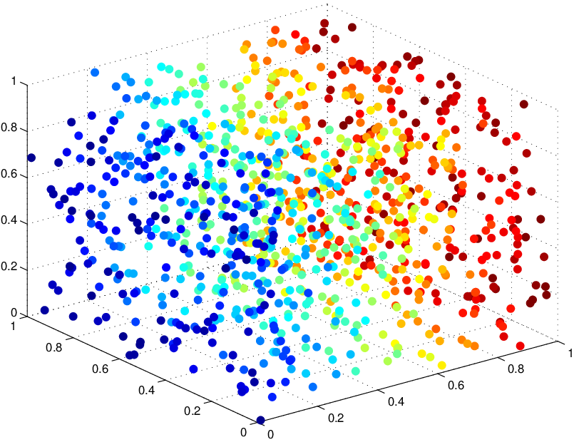
Data set #1 and #2: The sets of observation locations vary from 1,000 to 512,000 and we assume that for for and . The observations locations are sampled from a uniform distribution over the unit square for (data set #1) and for for (data set #2), as shown in Figure 8. The target points are set to 1000 random points across the domain (data set #1) and (data set #2). We shall refer to as the observation values associated with .
Data set #3: We take the data set generated by for (256,000 observation points) and carve out two disks located at (1/4,1/4) and (3/4,3/4) with radii 1/4. This generates 100,637 observation points; see Figure 8(c) for an example with 1,562 observation points randomly extracted from the data set.
We now test our approach on the Matérn covariance function , where is the gamma function and is the modified Bessel function of the second kind. All results are executed on a single CPU (4 core Intel i7-3770 CPU @ 3.40GHz.) with Linux Ubuntu 13.04.
 |
 |
 |
| (a) | (b) | (c) |
7.1 Parameter Estimation
In this section we present the results for data set #1 and #3 for the Matérn parameter estimation.
Suppose we have two realizations of the Gaussian spatial random field with the Matérn covariance for data set #1 (2D). We set () and (corresponding to ) and fix the covariance parameters to . Two realizations () and () are generated from these parameters. For each observation values and (and locations) apply the transformation to compute and and solve the optimization problems for and .
Estimation results for data set #1 (2D).
| size() | ||||||||||
| 64,000 | 6 | 6 | 28 | -0.0759 | 0.0333 | 8.9 | 23 | 14 | 0 | |
| 64,000 | 6 | 5 | 28 | 0.0182 | -0.0132 | 1.7 | 35328 | 40 | 1 | |
| 64,000 | 6 | 4 | 28 | -0.0043 | 0.0046 | 4.5 | 56832 | 230 | 11 | |
| 64,000 | 6 | 3 | 28 | -0.0049 | 0.0048 | 10.7 | 62208 | 961 | 65 | |
| 64,000 | 5 | 6 | 21 | 0.0071 | -0.0146 | 0.4 | 810 | 13 | 0 | |
| 64,000 | 5 | 5 | 21 | 0.0037 | -0.0027 | 1.7 | 42496 | 43 | 2 | |
| 64,000 | 5 | 4 | 21 | -0.0030 | 0.0048 | 3.7 | 58624 | 220 | 12 | |
| 64,000 | 5 | 3 | 21 | -0.0048 | 0.0046 | 7.0 | 62656 | 750 | 32 | |
| 64,000 | 4 | 6 | 15 | -0.0080 | 0.0098 | 0.2 | 7749 | 13 | 0 | |
| 64,000 | 4 | 5 | 15 | -0.0047 | 0.0043 | 2.0 | 48640 | 53 | 3 | |
| 64,000 | 4 | 4 | 15 | -0.0068 | 0.0062 | 3.4 | 60160 | 161 | 9 | |
| 64,000 | 4 | 3 | 15 | -0.0051 | 0.0048 | 4.4 | 63040 | 550 | 15 | |
| 128,000 | 6 | 6 | 28 | 0.0010 | -0.0011 | 0.3 | 17179 | 75 | 0 | |
| 128,000 | 6 | 5 | 28 | 0.0025 | -0.0020 | 2.1 | 99328 | 350 | 13 | |
| 128,000 | 6 | 4 | 28 | -0.0002 | 0.0005 | 4.0 | 120832 | 1200 | 70 | |
| 128,000 | 5 | 6 | 21 | -0.0010 | 0.0015 | 0.5 | 42154 | 80 | 0 | |
| 128,000 | 5 | 5 | 21 | 0.0004 | -0.0002 | 1.9 | 106496 | 300 | 14 | |
| 128,000 | 5 | 4 | 21 | -0.0016 | 0.0017 | 3.3 | 122624 | 1000 | 50 |
Estimation results for data set #3 (2D).
| size() | ||||||||||
|---|---|---|---|---|---|---|---|---|---|---|
| 100,637 | 6 | 6 | 66 | 0.0548 | -0.0237 | 0.5 | 2613 | 60 | 0 | |
| 100,637 | 6 | 5 | 66 | -0.0031 | 0.0020 | 3.1 | 72231 | 600 | 12 |
The optimization problem from the log-likelihood function (6) is solved using fminsearch from the optimization toolbox in MATLAB with the local minimizer search for in the interval and in the interval . We set the parameter criterion to , and the fminsearch tolerance is set to . In Table 2 we tabulate the results for the parameter estimates and for different problem sizes of data sets #1 and #3 for the user defined parameters for the construction of the MB and for the construction of the matrix . We notice that the estimates of seem to approach the actual values as we increase the number of observations. In particular, for the estimate is very close to the actual noise model parameters of the covariance function. We observe that as we increase the number of levels (i.e. decrease ) in the covariance matrix the absolute error decays until it stagnates, usually by the time that the covariance matrix is for two levels. We also report the wall clock times (i.e. actual time it took the executable to run, not to be confused with CPU time that is unreliable as a measure) for computing each Newton iteration. The total number of Newton iterations is approximately 50.
In Table 2 the results for parameter estimation with data set #3 are tabulated. The realization is obtained from the Gaussian random field with , and . For this case the absolute error is 0.25% for the estimate and 0.04% for .
Statistical results for data set #1 with multiple realizations.
| 32,000 | 4 | 5 | 15 | 5 | |||||
| 32,000 | 4 | 4 | 15 | 5 | |||||
| 32,000 | 4 | 3 | 15 | 5 | |||||
| 64,000 | 4 | 6 | 15 | 6 | |||||
| 64,000 | 4 | 5 | 15 | 6 | |||||
| 64,000 | 4 | 4 | 15 | 6 | |||||
| 128,000 | 6 | 6 | 28 | 6 | |||||
| 128,000 | 6 | 5 | 28 | 6 |
In Table 3 we generate realizations of the stochastic model for data set #1, to analyze the mean and standard deviation of the Matérn covariance parameter estimates. The mean estimate refers to the mean of estimates for the the realizations of the stochastic model. Similarly, refers to the the standard deviation of the realizations. We observe that the mean appears to approach the covariance parameters as we decrease . As is reduced from to there is a significant drop in the term . However, for the standard deviation does not improve significantly. Therefore, there is not much gain in improving the estimate by decreasing , which increases the computational cost in computing .
7.2 Numerical examples for computing and Kriging
We test our approach for solving the system of equations (that we have to solve to obtain the kriging predictor) on the data sets #1 and #2. We also include results showing the kriging prediction error between the multi-level and direct methods.
We first test the PCG method with data set #2 (3D) on three test cases: (a) , (b) and (c) . The value gives us an approximate decay of (which is reasonable in practice) from the center of the cube along each dimensional axis. The PCG relative error tolerance is set to a value that leads to a relative error of the unpreconditioned system .
In Table 4 we report the total wall clock times and iterations for computing , and the target for data set #2 (3D) with the Matérn covariance function . The polynomial accuracy of the model is set to cubic (, ) and the accuracy parameter is set to 20 (which corresponds to ). We look at three cases: For (a) () we set the KIFMM accuracy to medium and the number of iterations increase as . For (b) () we set the KIFMM accuracy to medium and the number of iterations increases as . For (c) () we set the KIFMM accuracy to high and the number of iterations increases as .
In Table 4 we also report the number of iterations needed for solving with accuracy with a CG method. In this case the number of iterations is about 10 times larger than the multi-level version. Moreover, for solving the kriging problem (e.g. equation (4)), such problems have to be solved. Thus, it is at least about 200 times faster since for this case. An alternative is to solve (6). However, in general it is not positive definite. The matrix is highly ill-conditioned also making it difficult to solve with an iterative solver such as generalized minimal residual method (see Castrillón-Candás et al. (2013)).
(a) , , (), ()
| itr() | itr() | Diag. (s) | Itr (s) | Total (s) | ||
|---|---|---|---|---|---|---|
| 16,000 | 166 | 1296 | 80 | 113 | 193 | |
| 32,000 | 247 | 3065 | 215 | 321 | 536 | |
| 64,000 | 372 | 5517 | 665 | 1226 | 1891 | |
| 128,000 | 547 | - | 2060 | 3237 | 5397 | |
| 256,000 | 847 | - | 5775 | 9885 | 15660 | |
| 512,000 | 1129 | - | 17896 | 33116 | 51012 |
(b) , , (), ()
| itr() | itr() | Diag. (s) | Itr (s) | Total (s) | ||
|---|---|---|---|---|---|---|
| 16,000 | 293 | 2970 | 79 | 198 | 277 | |
| 32,000 | 470 | 7786 | 213 | 607 | 820 | |
| 64,000 | 760 | 15808 | 662 | 2495 | 3157 | |
| 128,000 | 1167 | - | 2050 | 7109 | 9159 | |
| 256,000 | 1961 | - | 5789 | 22878 | 28667 |
(c) , , (), ()
| itr() | itr() | Diag. (s) | Itr (s) | Total (s) | ||
|---|---|---|---|---|---|---|
| 16,000 | 500 | 5953 | 138 | 580 | 718 | |
| 32,000 | 827 | 17029 | 346 | 1574 | 1920 | |
| 64,000 | 1567 | 37018 | 910 | 6474 | 7384 | |
| 128,000 | 2381 | - | 3974 | 25052 | 29026 | |
| 256,000 | 4299 | - | 10322 | 72374 | 82696 |
In Table 5 the results for computing , and for 1000 target points for data set #1 (2D) with the Matérn covariance function are tabulated. We have three test cases: (a) (note for this case we obtain an exponential covariance function), (b) , and (c) . For (a) and (b) the KIFMM accuracy is set to medium. For (c) the KIFMM accuracy is set to high. For this case the relative residual accuracy for the unpreconditioned system is fixed at .
We note that for this case the results are even more impressive than for the 3D case. For Table 5 (c) the CG solver stagnated and we terminated the iteration after 100,000. At this point the matrix is highly ill-conditioned. In contrast, with we are still able to solve the problem even for 128,000 size problem.
(a) , , (), ()
itr()
itr()
Diag. (s)
Itr (s)
Total (s)
16,000
330
3603
246
115
361
32,000
333
5429
750
251
1001
64,000
455
8152
1947
589
2536
128,000
564
-
5570
1577
7147
256,000
619
-
15266
3065
18331
512,000
1230
-
42254
13101
55355
(b) , , (), ()
| itr() | itr() | Diag. (s) | Itr (s) | Total (s) | ||
|---|---|---|---|---|---|---|
| 16,000 | 965 | 26795 | 370 | 397 | 767 | |
| 32,000 | 1110 | 41079 | 1125 | 1061 | 2186 | |
| 64,000 | 2239 | 82166 | 2892 | 3714 | 6606 | |
| 128,000 | 3443 | - | 8268 | 13130 | 21398 | |
| 256,000 | 4557 | - | 23175 | 30302 | 53477 |
(c) , , (), ()
itr()
itr()
Diag. (s)
Itr (s)
Total (s)
16,000
2710
553
1844
2397
32,000
4261
-
1522
5713
7235
64,000
8801
-
5022
23785
28807
128,000
14405
-
12587
75937
88524
The diagonal preconditioner we use is one of the simplest. We plan to extend this approach to more sophisticated preconditioners such as block Symmetric Successive OverRelaxation (SSOR) (see Castrillón-Candás et al. (2013)) in the future.
The residual errors are then propagated to the final estimate around the same magnitude. However, as a final experiment in Table 6 we tabulate the relative error between the multi-level kriging approach and the direct method for data set #2 with exponential covariance function , where and . The PCG tolerance is set to and . Notice that the error increases with . This is expected since the unpreconditioned system error will degrade.
| Relative Error | |
|---|---|
| 1,000 | |
| 2,000 | |
| 4,000 | |
| 8,000 | |
| 16,000 | |
| 32,000 |
8 Conclusions
In this paper we developed a multi-level restricted Gaussian maximum likelihood method for estimating the covariance function parameters and the computation of the best unbiased predictor. Our approach produces a new set of multi-level contrasts that decouples the covariance parameters from the deterministic components. In addition, the covariance matrix exhibits fast decay independently from the decay rate of the covariance function. Due to the fast decay of the covariance matrix only a small set of coefficients of the covariance matrix are computed with a level-dependent criterion. We showed results of our method for the Matérn covariance with highly irregular placement of the observation locations to good accuracy.
We are currently working on deriving error estimates of the kriging estimate and determinant computation with respect to the number of degrees of freedom . We are also contemplating extending our multi-level approach to multivariate random fields and cokriging (e.g. Furrer and Genton (2011)).
Our method also applies to non-stationary problems if the covariance function is differentiable to degree . For example, if the covariance function changes smoothly with respect to the location, Lemma 10 still applies and the multi-level covariance matrix decays at the same rate as a stationary one. Now, even if the covariance function is non differentiable everywhere with respect to the location, Lemma 10 still applies, but at a lower decay rate.
Note that we have not made direct comparisons with many of the approaches described in Section 1. These methods are very good at solving a particular type of problem i.e. grid-like geometries and/or compact covariance functions. For these situations we recommend using the approaches already developed in the literature as they work well and are easier to implement. However, to our knowledge we have no seen fast results where the placement of the observations are highly irregular and the Matérn covariance function decays slowly. We plan to include some comparison for the spatial covariance paper we plan to write.
Appendix A: Proofs
Lemma 10:
Since is in , then by Taylor’s theorem we have that for every , where , , and for some . Now, recall that is orthogonal to then . Since is also orthogonal to then by applying Taylor’s theorem centered at :
for some . The last inequality follows since from Schwartz’ inequality and .
Lemma 2: Since the Matérn covariance function is positive definite we have that for all :
where is the entry of the matrix . The diagonal terms of are of the form . This implies that
Thus, will always be positive definite.
Appendix B: Notation
| Index for when the following are first defined, mentioned or reformulated. | |||
|---|---|---|---|
| Dimension of problem (p1) | Number of observations (p1) | ||
| Maximum MB level (p8) | Number of columns of (p1) | ||
| Polynomial degree (p7) | Accuracy parameter of MB (p7) | ||
| Degree of multilevel basis. p(7) | Dimension of (p1) | ||
| Design matrix (p1) | Covariance function (p7) | ||
| Locations of observations (p1) | Param. of matern kernel (p1) | ||
| Covariance matrix (p1) | Observation values (p1) | ||
| Target points set (p1) | Span of the columns of (p1) | ||
| Vector of unknowns from | , | Estimates | |
| deterministic model (p1) | kriging estimate at (p2) | ||
| Log-likelihood function (p1) | Cube at level and index (p8) | ||
| (p4) | (p4) | ||
| (p10) | (p17) | ||
| Multilevel log-likelihood (p17) | |||
| Set of polynomial monomials | Level dependent | ||
| of order and dimension (p7) | criterion constant (p13) | ||
Appendix C
Using the approach developed in this paper we can compute the MSE at the target point . Now, since we have that , , where and . Let , then
Given that then . Following a similar argument we have that equation (20) becomes
| (22) |
where . By using matrix-vector products with the
PCG method
can be computed in . Thus the term can be computed in . Now, by
also using matrix-vector products the term
can be computed in . Thus the total cost for computing equation (22) is
.
Acknowledgements: We appreciate the help and advice from Jun Li and Lisandro Dalcin in getting the C++ code working properly, and to Stefano Castruccio for giving us feedback on our manuscript.
References
- Anitescu et al. (2012) Anitescu, M., Chen, J., and Wang, L. (2012), “A Matrix-Free Approach for Solving the Parametric Gaussian Process Maximum Likelihood Problem,” SIAM Journal on Scientific Computing, 34, 240–262.
- Balay et al. (2013a) Balay, S., Brown, J., Buschelman, K., Eijkhout, V., Gropp, W. D., Kaushik, D., Knepley, M. G., McInnes, L. C., Smith, B. F., and Zhang, H. (2013a), “PETSc Users Manual,” Tech. Rep. ANL-95/11 - Revision 3.4, Argonne National Laboratory.
- Balay et al. (2013b) Balay, S., Brown, J., Buschelman, K., Gropp, W. D., Kaushik, D., Knepley, M. G., McInnes, L. C., Smith, B. F., and Zhang, H. (2013b), “PETSc Web Page,” Http://www.mcs.anl.gov/petsc.
- Balay et al. (1997) Balay, S., Gropp, W. D., McInnes, L. C., and Smith, B. F. (1997), “Efficient Management of Parallelism in Object Oriented Numerical Software Libraries,” in Modern Software Tools in Scientific Computing, eds. Arge, E., Bruaset, A. M., and Langtangen, H. P., Birkhäuser Press, pp. 163–202.
- Beatson and Greengard (1997) Beatson, R. and Greengard, L. (1997), “A Short Course on Fast Multipole Methods,” in Wavelets, Multilevel Methods and Elliptic PDEs, Oxford University Press, pp. 1–37.
- Castrillón-Candás et al. (2013) Castrillón-Candás, J., Li, J., and Eijkhout, V. (2013), “A Discrete Adapted Hierarchical Basis Solver for Radial Basis Function Interpolation,” BIT Numerical Mathematics, 53, 57–86.
- Chen et al. (2008) Chen, Y., Davis, T. A., Hager, W. W., and Rajamanickam, S. (2008), “Algorithm 887: CHOLMOD, Supernodal Sparse Cholesky Factorization and Update/Downdate,” ACM Trans. Math. Softw., 35, 22:1–22:14.
- Davis and Hager (1999) Davis, T. and Hager, W. (1999), “Modifying a Sparse Cholesky Factorization,” SIAM Journal on Matrix Analysis and Applications, 20, 606–627.
- Davis and Hager (2001) — (2001), “Multiple-Rank Modifications of a Sparse Cholesky Factorization,” SIAM Journal on Matrix Analysis and Applications, 22, 997–1013.
- Davis and Hager (2005) — (2005), “Row Modifications of a Sparse Cholesky Factorization,” SIAM Journal on Matrix Analysis and Applications, 26, 621–639.
- Davis and Hager (2009) Davis, T. A. and Hager, W. W. (2009), “Dynamic Supernodes in Sparse Cholesky Update/Downdate and Triangular Solves,” ACM Trans. Math. Softw., 35, 27:1–27:23.
- Elden et al. (2004) Elden, L., Wittmeyer-Koch, L., and Nielsen, H. (2004), Introduction to Numerical Computation - analysis and Matlab illustrations, Studentlitteratur.
- Furrer and Genton (2011) Furrer, R. and Genton, M. G. (2011), “Aggregation-Cokriging for Highly-Multivariate Spatial Data,” Biometrika, 98, 615–631.
- Furrer et al. (2006) Furrer, R., Genton, M. G., and Nychka, D. (2006), “Covariance Tapering for Interpolation of Large Spatial Datasets,” Journal of Computational and Graphical Statistics, 15, 502–523.
- George (1973) George, A. (1973), “Nested Dissection of a Regular Finite Element Mesh,” SIAM Journal on Numerical Analysis, 10, 345–363.
- Gilbert and Tarjan (1987) Gilbert, J. R. and Tarjan, R. E. (1987), “The Analysis of a Nested Dissection Algorithm,” Numerische Mathematik, 50, 377–404.
- Kaufman et al. (2008) Kaufman, C. G., Schervish, M. J., and Nychka, D. W. (2008), “Covariance Tapering for Likelihood-Based Estimation in Large Spatial Datasets,” Journal of the American Statistical Association, 103, 1545–1555.
- Stein et al. (2012) Stein, M. L., Chen, J., and Anitescu, M. (2012), “Difference Filter Preconditioning for Large Covariance Matrices,” SIAM Journal on Matrix Analysis and Applications, 33, 52–72.
- Stein et al. (2013) — (2013), “Stochastic Approximation of Score Functions for Gaussian Processes,” Annals of Applied Statistics, 7, 1162–1191.
- Stein et al. (2004) Stein, M. L., Chi, Z., and Welty, L. J. (2004), “Approximating Likelihoods for Large Spatial Data Sets,” Journal of the Royal Statistical Society, Series B, 66, 275–296.
- Sun et al. (2012) Sun, Y., Li, B., and Genton, M. G. (2012), “Geostatistics for Large Datasets,” in Space-Time Processes and Challenges Related to Environmental Problems, eds. Porcu, M., Montero, J. M., and Schlather, M., Springer, pp. 55–77.
- Sun and Stein (2015) Sun, Y. and Stein, M. L. (2015), “Statistically and Computationally Efficient Estimating Equations for Large Spatial Datasets,” Journal of Computational and Graphical Statistics, Posted online 07 Nov 2014.
- Ying et al. (2004) Ying, L., Biros, G., and Zorin, D. (2004), “A Kernel-Independent Adaptive Fast Multipole Method in Two and Three Dimensions,” Journal of Computational Physics, 196, 591–626.