跳到论文正文
W Papers独立论文阅读器 arXiv:1503.09139 论文正文 计算阅读时间 · 0%
引用这篇论文根据当前论文元数据生成,正式投稿前建议核对。


License: arXiv.org perpetual non-exclusive license
arXiv:1503.09139v2 [cond-mat.str-el] 09 Dec 2015

Steady-state dynamics and effective temperatures of quantum criticality in an open system

P. Ribeiro Affiliation: Russian Quantum Center, Novaya street 100 A, Skolkovo, Moscow area, 143025 Russia Affiliation: Centro de Física das Interacções Fundamentais, Instituto Superior Técnico, Universidade de Lisboa, Av. Rovisco Pais, 1049-001 Lisboa, Portugal    F. Zamani Affiliation: Max Planck Institute for Physics of Complex Systems, 01187 Dresden, Germany Affiliation: Max Planck Institute for Chemical Physics of Solids, 01187 Dresden, Germany    S. Kirchner Email: stefan.kirchner@correlated-matter.com Affiliation: Center for Correlated Matter, Zhejiang University, Hangzhou, Zhejiang 310058, China
Abstract

We study the thermal and non-thermal steady state scaling functions and the steady-state dynamics of a model of local quantum criticality. The model we consider, i.e. the pseudogap Kondo model, allows us to study the concept of effective temperatures near fully interacting as well as weak-coupling fixed points. In the vicinity of each fixed point we establish the existence of an effective temperature –different at each fixed point– such that the equilibrium fluctuation-dissipation theorem is recovered. Most notably, steady-state scaling functions in terms of the effective temperatures coincide with the equilibrium scaling functions. This result extends to higher correlation functions as is explicitly demonstrated for the Kondo singlet strength. The non-linear charge transport is also studied and analyzed in terms of the effective temperature.

pacs
05.70.Jk,05.70.Ln,64.70.Tg,72.10.Fk

The interest in understanding the dynamics of strongly correlated systems beyond the linear response regime has in recent years grown tremendously.
The quantum dynamics in adiabatically isolated optical traps has been successfully modeled using powerful numerical schemes [1, 2]. In open systems mainly diagrammatic techniques on the Schwinger-Keldysh contour have been employed. For nanostructured systems several techniques exist to describe the ensuing out-of-equilibrium properties. These approaches, however, are either perturbative in nature [3], centered around high temperatures and short times [4, 5, 6, 7, 8], or approximate the continuous baths by discrete Wilson chains [9, 10, 11]. The situation might be simpler for non-linear dynamics that arises in the vicinity of a quantum critical point (QCP), where a vanishing energy scale leads to scaling and universality [12, 13, 14, 15, 16, 17, 18, 19].
For the dynamics near classical continuous phase transitions a well-established theoretical framework exists, tying the dynamics to the statics and the conserved quantities [20]. In addition, the concept of effective temperature (Teff {}_{\mbox{\tiny eff\penalty\ }}) was established as an useful notion for the relaxational dynamics of classical critical systems [21, 22, 23, 24], although it appears somewhat less useful for fully interacting critical points [23]. Teff {}_{\mbox{\tiny eff\penalty\ }}is commonly defined by extending the equilibrium fluctuation-dissipation theorem to the non-linear regime. The existence of effective temperatures in quantum systems was recently investigated [25, 26, 27, 28, 18]. For a recent review see [25]. In comparison to classical criticality, at a QCP, dynamics already enters at the equilibrium level. For a QCP that can be described by a Ginzburg-Landau-Wilson functional in elevated dimensions, it was found that the voltage-driven transition is in the universality class of the associated thermal classical model with voltage acting as Teff {}_{\mbox{\tiny eff\penalty\ }} [12]. Unconventional QCPs in contrast are not described solely in terms of an order parameter functional [29, 30].

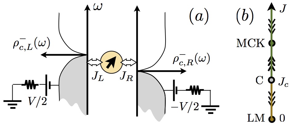
In this letter we address the following general questions within a model system of unconventional quantum criticality: Is the existence of Teff {}_{\mbox{\tiny eff\penalty\ }}tied to dynamical (or ω/T\omega/T-)scaling? Does Teff {}_{\mbox{\tiny eff\penalty\ }}have meaning for higher correlation functions? How unique is Teff {}_{\mbox{\tiny eff\penalty\ }}at a given fixed point once boundary conditions have been specified? Can critical scaling functions be expressed through Teff {}_{\mbox{\tiny eff\penalty\ }}and if so, how do these scaling functions relate to the equilibrium scaling functions? The model system is the pseudogap Kondo (pKM) model that describes a quantum spin anti-ferromagnetically coupled to a conduction electron bath possessing a pseudogap near its Fermi energy, characterized by a powerlaw exponent. Depending on the coupling strength, the quantum spin is either screened or remains free in the zero temperature (TT) limit. The two phases are separated by a critical point dispaying critical Kondo destruction, see Fig.1. The pKM has been invoked to describe non-magnetic impurities in the cuprate superconductors [31] and point-defects in graphene [32]. It underlies the pseudogap free moment phases occurring in certain disordered metals [33] and can also be realized in double quantum-dot systems [34]. The quantum critical properties of the pKM in equilibrium have been addressed in [35, 36, 37, 38, 39, 40, 41, 42, 43, 44, 45]. Our main findings are that the steady state dynamic spin susceptibility, the conductance, and the Kondo-singlet strength, a 4-point correlator, reproduce their equilibrium behavior in the scaling regimes of the fixed points of the model when expressed in terms of a fixed-point specific Teff {}_{\mbox{\tiny eff\penalty\ }}.
The model. We consider a pKM with a density of states that vanishes in a power-law fashion with exponent 0≤r≤10\leq r\leq 1 at their respective Fermi level, ρc,l−​(ω)∼|ω|r​Θ​(D−|ω|)\rho_{c,l}^{-}(\omega)\sim|\omega|^{r}\Theta(D-|\omega|), with half-bandwidth DD. Here, l=L,Rl=L,R labels the two leads, see Fig.1(a). In the multichannel version of the model the spin degree of freedom (𝑺\boldsymbol{S}) is generalized from S​U​(2)SU(2) to S​U​(N)SU(N) and the fermionic excitations (cc) of the leads transform under the fundamental representation of S​U​(N)×S​U​(M)SU(N)\times SU(M) with NN spin and MM charge channels. At T=0T=0 and r<rmax<1r<r_{\mbox{\tiny max}}<1, a critical point (C) separates a multichannel Kondo (MCK)-screened phase from a local moment (LM) phase at a critical value JcJ_{c} of the exchange coupling J>0J>0, see Fig.1(b). The characterization of the phases and the leading power law exponents of observables of the pKM have been obtained by perturbative RG, large-NN methods, and NRG [35, 37, 38, 43, 36, 37, 40]. Within the large-NN approach, at T=0T=0, scaling arguments are able to predict the critical exponents of dynamical observables [39, 46]. Non-equilibrium steady-states (NESS) are obtained by applying a time-independent bias voltage V=(μL−μR)/|e|V=(\mu_{L}-\mu_{R})/\left|e\right|, where μl\mu_{l} is the chemical potential of lead ll, see Fig. 1(a). As TT characterizes the fermionic reservoirs, it remains well-defined even for V≠0V\neq 0.
A similar setup has been considered in a perturbative RG-like study adapted to the NESS condition [47]. This model has also been invoked in a variational study of the dynamics following a local quench where it was found that quenches in the Kondo phase thermalize while this in not the case for quenches across the QCP into the LM regime [48].

Refer to caption
Figure 1: (a) Sketch of the model: a spin interacts with two fermionic leads which are characterized by their respective density of states ρc,L/R−​(ω)\rho_{c,L/R}^{-}\left(\omega\right) and chemical potential μL/R\mu_{L/R}. (b) Phase diagram of the multichannel pKM with gap exponent r<rmaxr<r_{\mbox{\tiny max}}: A QCP (C) separates the multichannel Kondo fixed point (MCK) from the (weak-coupling) local moment fixed point (LM).

The system is described by the Hamiltonian

H\displaystyle H =\displaystyle= ∑p,α​σ​lεp​l​cp​α​σ​l†​cp​α​σ​l+1N​∑l​l′∑αJl​l′​𝐒.𝐬α;l​l′,\displaystyle\sum_{p,\alpha\sigma l}\varepsilon_{pl}c_{p\alpha\sigma l}^{\dagger}c_{p\alpha\sigma l}+\frac{1}{N}\sum_{ll^{\prime}}\sum_{\alpha}J_{ll^{\prime}}\mathbf{S}.\mathbf{s}_{\alpha;ll^{\prime}}, (1)

where σ=1,…,N\sigma=1,\ldots,N and α=1,…,M\alpha=1,\ldots,M are, respectively, the S​U​(N)SU(N)-spin and S​U​(M)SU(M)-channel indices, ll labels the leads and pp is a momentum index. The co-tunneling term [49] in Eq. (1) contains the local operators 𝐬α;l​l′i=1nc​∑p​p′​σ​σ′cp​α​σ​l†​tσ​σ′i​cp′​α​σ′​l′†\mathbf{s}_{\alpha;ll^{\prime}}^{i}=\frac{1}{n_{c}}\sum_{pp^{\prime}\sigma\sigma^{\prime}}c_{p\alpha\sigma l}^{\dagger}t_{\sigma\sigma^{\prime}}^{i}c_{p^{\prime}\alpha\sigma^{\prime}l^{\prime}}^{\dagger} with tt the fundamental representation of S​U​(N)SU(N) and ncn_{c} is the number of fermionic single-particle states. In a totally anti-symmetric representation, one can decompose the spin operator as Sσ​σ′=fσ†​fσ′−q​δσ​σ′S_{\sigma\sigma^{\prime}}=f^{\dagger}_{\sigma}f_{\sigma^{\prime}}-q\delta_{\sigma\sigma^{\prime}}, where qq is subject to the constraint Q^=∑σfσ†​fσ=q​N\hat{Q}=\sum_{\sigma}f_{\sigma}^{\dagger}f_{\sigma}=qN and the fσ†,fσ′f_{\sigma}^{\dagger},f_{\sigma^{\prime}} obey fermionic commutation relations.

We employ a dynamical large-N limit [50, 39], suitably generalized to the Keldysh contour [16, 18] while keeping q=QNq=\frac{Q}{N} and κ=M/N\kappa=M/N constant. This results in

ΣB>,<​(t)\displaystyle\Sigma_{B}^{>,<}\left(t\right) =\displaystyle= i​Gf>,<​(t)​Gc<,>​(−t)\displaystyle iG_{f}^{>,<}\left(t\right)G_{c}^{<,>}\left(-t\right) (2)
Σf>,<​(t)\displaystyle\Sigma_{f}^{>,<}\left(t\right) =\displaystyle= −i​κ​GB>,<​(t)​Gc>,<​(t)\displaystyle-i\kappa G_{B}^{>,<}\left(t\right)G_{c}^{>,<}\left(t\right) (3)
−i​Gf<​(0)\displaystyle-iG_{f}^{<}\left(0\right) =\displaystyle= q,\displaystyle q, (4)

where GfG_{f} is the pseudofermion propagator and GBG_{B} is the propagator of a bosonic Hubbard-Stratonovich decoupling field. Σf\Sigma_{f} (ΣB\Sigma_{B}) is the proper selfenergy of GfG_{f} (GBG_{B}) and is related to it via the Dyson equation [51]. We assume that the exchange interaction originates from an Anderson-type model via a Schrieffer-Wolff transformation, so that a single coupling constant J=JL+JRJ=J_{L}+J_{R} emerges [51].
For details on the numerics see [51]. In equilibrium, our approach yields dynamical scaling functions that coincide with those obtained from quantum Monte-Carlo [44].

Refer to caption
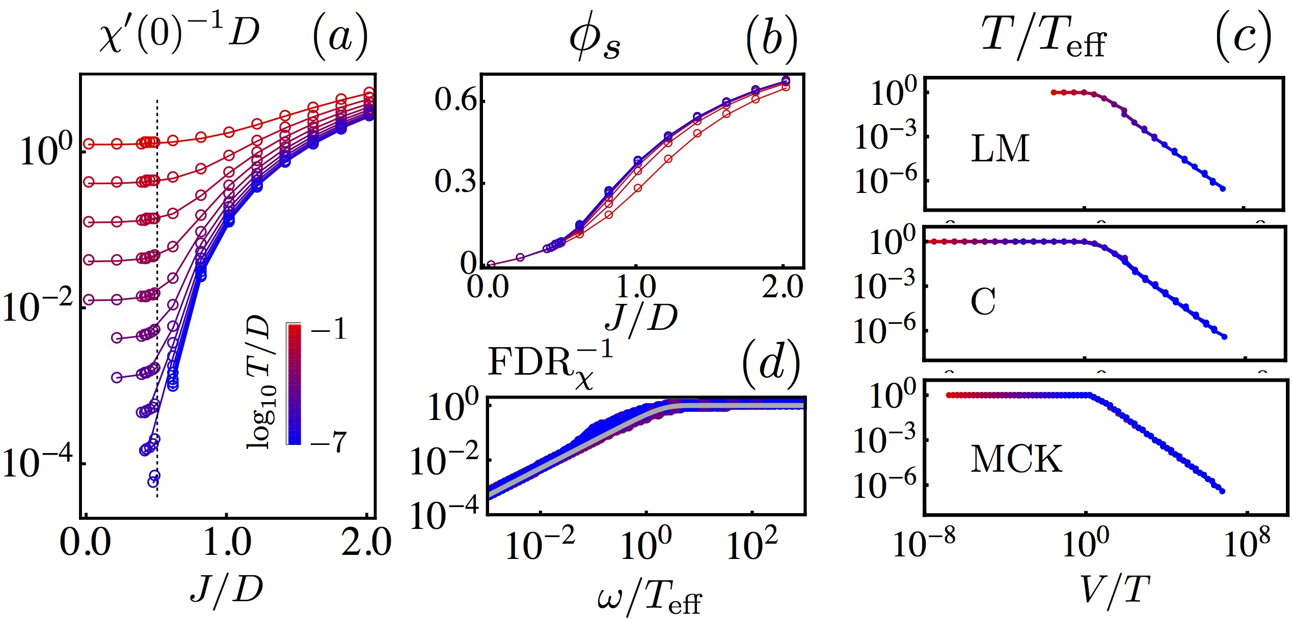
Figure 2: (a) χ′​(0)−1\chi^{\prime}\left(0\right)^{-1}vs JJ for different TT. (b) ϕs\phi_{s} vs JJ for different TT. The T=0T=0 curve is approached from below in the MCK and from above in the LM phases. (c) Scaling T/TeffT/T_{\mbox{\tiny eff}} vs V/TV/T at fixed points LM, C, and MCK: Teff∼VT_{\mbox{\tiny eff}}\sim V for V≫TV\gg T. (d) FDRχ−1​(ω)\text{FDR}^{-1}_{\chi}(\omega) vs ω/Teff\omega/T_{\text{eff}} near fixed point C, shown for V/D=10−2,10−3,10−4,10−5,10−6V/D=10^{-2},10^{-3},10^{-4},10^{-5},10^{-6}. The grey line is FDR−1​(ω)=tanh⁡(β​ω/2)\text{FDR}^{-1}(\omega)=\tanh(\beta\omega/2).

Observables. A possible order parameter for the transition from the overscreened Kondo to local-moment phase is given by limT→0T​χ​(ω=0,T)\lim_{T\rightarrow 0}T\chi(\omega=0,T), where χ⁡(ω,T)\chi(\omega,T) is the Fourier transform of the local (impurity) spin-spin correlation function χ⁡(t−t′)\chi(t-t^{\prime}), see Fig. 2(a). We work on the Keldysh contour where the lesser and greater components are defined in the usual way as χ>(t−t′)=−i1N∑a⟨Sa(t)Sa(t′)⟩\chi^{>}\left(t-t^{\prime}\right)=-i\frac{1}{N}\sum_{a}\left\langle S^{a}\left(t\right)S^{a}\left(t^{\prime}\right)\right\rangle with t∈γ←t\in\gamma_{\leftarrow} and t′∈γ→t^{\prime}\in\gamma_{\rightarrow} and χ<(t−t′)=−i1N∑a⟨Sa(t′)Sa(t)⟩\chi^{<}\left(t-t^{\prime}\right)=-i\frac{1}{N}\sum_{a}\left\langle S^{a}\left(t^{\prime}\right)S^{a}\left(t\right)\right\rangle, with t∈γ→t\in\gamma_{\rightarrow} and t′∈γ←t^{\prime}\in\gamma_{\leftarrow} so that χR​(t)=Θ⁡(t)​[χ>​(t)−χ<​(t)]\chi^{R}\left(t\right)=\Theta\left(t\right)\left[\chi^{>}\left(t\right)-\chi^{<}\left(t\right)\right] and χA=χR+χ<−χ>\chi^{A}=\chi^{R}+\chi^{<}-\chi^{>}. Here, γ→(←)\gamma_{\rightarrow(\leftarrow)} is the forward (backward) branch of the Keldysh contour, respectively.

We also consider the “singlet-strength” ϕs\phi_{s}, defined through the Kondo term contribution to the total energy of the system as 1N∑l​l′∑cJl​l′⟨𝐒.𝐬c,l​l′⟩=−Jκ(N2−1N)ϕs\frac{1}{N}\sum_{ll^{\prime}}\sum_{c}J_{ll^{\prime}}\left\langle\mathbf{S}.\mathbf{s}_{c,ll^{\prime}}\right\rangle=-J\kappa\left(\frac{N^{2}-1}{N}\right)\phi_{s} [52]. ϕs\phi_{s} is a dimensionless quantity, which possesses a well-defined large-NN limit and quantifies the degree of singlet formation. In terms of the fermionic fields, it can be written as the local-in-time limit of a 4-point correlator [51]. Its equilibrium properties will be discussed below. The steady state charge current passing through each channel is 𝒥P=−∂t⟨N^L(t)⟩/M\mathcal{J}_{\text{P}}=-\partial_{t}\left\langle\hat{N}_{L}\left(t\right)\right\rangle/M, where N^L=∑p​α​σcp​α​σ​L†​cp​α​σ​L\hat{N}_{L}=\sum_{p\alpha\sigma}c_{p\alpha\sigma L}^{\dagger}c_{p\alpha\sigma L} is the number of particles in the left lead. The out-of-equilibrium conditions considered here respect particle-hole symmetry which implies a vanishing energy current.

Throughout the paper we set κ=0.3\kappa=0.3, r=0.2r=0.2, and q=1/2q=1/2. This results in rmax=0.412​(4)r_{\mbox{\tiny max}}=0.412(4). Our choice of values for κ\kappa and rr ensures a finite static spin susceptibility χ′​(ω=0)\chi^{\prime}\left(\omega=0\right) within the MCK phase as T→0T\rightarrow 0. We denote the real (imaginary) part of χR​(ω)\chi^{R}(\omega) by χ′\chi^{\prime} (χ′′\chi^{\prime\prime}).

Refer to caption
Figure 3: Scaling of observables with TeffT_{\text{eff}} at different fixed points for the values of VV as in Fig. 2(d): (a) χ′​(0)−1\chi^{\prime}\left(0\right)^{-1}vs TeffT_{\text{eff}}; (b) ∂ln⁡ωln⁡χ′′​(ω)\partial_{\ln\omega}\ln\chi^{\prime\prime}\left(\omega\right) vs ω/Teff\omega/T_{\text{eff}}; (c) ϕs\phi_{s} vs TeffT_{\text{eff}}. For each fixed point, the equilibrium scaling form (grey curves) is compared with the same quantity under non-equilibrium conditions and TT substituted by TeffT_{\text{eff}}.

Thermal steady-state. The equilibrium (V=0V=0) behavior of χ′​(ω=0,T)\chi^{\prime}\left(\omega=0,T\right) in the relaxational regime (ω≪T\omega\ll T) near the MCK, C, and LM fixed points is shown in Fig.2-(a). For J<Jc≃0.44​DJ<J_{c}\simeq 0.44D, i.e. in the LM phase, one observes Curie-like behavior at lowest temperatures χ′​(ω=0,T)∝T−1\chi^{\prime}\left(\omega=0,T\right)\propto T^{-1}. In the MCK phase (J>JcJ>J_{c} and with our choices of κ\kappa and rr), the T=0T=0 susceptibility remains finite. The grey lines in Figs.3-(b) show the scaling plots of the logarithmic derivative of χ′′​(ω)\chi^{\prime\prime}\left(\omega\right) for different values of the temperature, i.e. ∂ln⁡ωln⁡χ′′​(ω)\partial_{\ln\omega}\ln\chi^{\prime\prime}\left(\omega\right) for the different fixed points. Note that ∂ln⁡ωln⁡χ′′​(ω)≃αχ\partial_{\ln\omega}\ln\chi^{\prime\prime}\left(\omega\right)\simeq\alpha_{\chi} within the scaling region where χ′′​(ω)∝|ω|αχ\chi^{\prime\prime}\left(\omega\right)\propto\left|\omega\right|^{\alpha_{\chi}}. The values of αχ\alpha_{\chi} in the quantum coherent regime (ω/T≫1\omega/T\gg 1) agree with those obtained analytically from a T=0T=0 scaling ansatz [46] for the MCK (αχ≃0.087\alpha_{\chi}\simeq 0.087) and C (αχ=−0.97\alpha_{\chi}=-0.97) fixed points. These results are compatible with a dynamical scaling form χ′′​(ω,T)=Tαχ​Φ​(ω/T)\chi^{\prime\prime}\left(\omega,T\right)=T^{\alpha_{\chi}}\Phi\left(\omega/T\right), in terms of an universal scaling function Φ⁡(x)\Phi\left(x\right) possessing asymptotic values Φ⁡(x)∝x\Phi\left(x\right)\propto x for x≪1x\ll 1 and Φ⁡(x)∝xαχ\Phi\left(x\right)\propto x^{\alpha_{\chi}} for x≫1x\gg 1. Thus, the scaling properties are in line with dynamical ω/T\omega/T-scaling for the C and MCK fixed points. For the LM fixed point we find αχ=−1\alpha_{\chi}=-1 and a scaling form χ′′​(ω)=Tαχ​Φ~​(ω/T1+κ)\chi^{\prime\prime}\left(\omega\right)=T^{\alpha_{\chi}}\widetilde{\Phi}\left(\omega/T^{1+\kappa}\right), indicative of a weak-coupling fixed point and absence of hyperscaling. These results will be further addressed elsewhere [46].
The singlet-strength ϕs\phi_{s} vs. JJ at different TT and at V=0V=0 is shown in Fig.2-(b). The numerical data at T≠0T\neq 0 suggest that ϕs​(J,T=0)\phi_{s}\left(J,T=0\right) is a continuous function of JJ. At the C fixed point we find that ϕs​(J,T)\phi_{s}\left(J,T\right) as a function of JJ crosses for different values of TT (for sufficiently low TT).
Non-thermal steady-states. We consider a non-equilibrium setup where the two leads, initially decoupled from the impurity (for t<t0t<t_{0}), are held at chemical potentials μL=−μR=|e|​V/2\mu_{L}=-\mu_{R}=\left|e\right|V/2 (|e|=1\left|e\right|=1 in the following). At t=t0t=t_{0} the coupling between the leads and the impurity is turned on. A steady-state is reached by sending t0→−∞t_{0}\to-\infty so that any transient behavior will already have faded away at (finite) time tt. The NESS fluctuation-dissipation ratio (FDR) for a dynamical observable A⁡(t,t′)=A⁡(t−t′)A(t,t^{\prime})=A(t-t^{\prime}) is defined through FDR(ω)A=[A>(ω)+A<(ω)]/[A>(ω)−A<(ω)]\text{FDR}{}_{A}(\omega)=[A^{>}(\omega)+A^{<}(\omega)]/[A^{>}(\omega)-A^{<}(\omega)], where A>/<A^{>/<} are the Fourier transforms of the greater/lesser components of AA. At equilibrium, the fluctuation-dissipation theorem implies FDRA​(ω)=tanh⁡(β​ω/2)ζ\text{FDR}_{A}(\omega)=\tanh\left(\beta\omega/2\right)^{\zeta} uniquely (with ζ=±1\zeta=\pm 1 for fermionic (+) and bosonic (-) operators). For a generic out-of-equilibrium system, the functional form of the FDR differs from the equilibrium one. A frequency-dependent “effective temperature”, 1/βeffA​(ω)1/\beta_{\text{eff}}^{A}\left(\omega\right), for the observable AA can be defined by requiring that tanh⁡[βeffA​(ω)​ω/2]ζ=FDRA​(ω)\tanh\left[\beta_{\text{eff}}^{A}\left(\omega\right)\omega/2\right]^{\zeta}=\text{FDR}_{A}(\omega) [53, 27]. Following Refs. [21, 26, 18] we define TeffT_{\mbox{\tiny eff}} via FDRχ\text{FDR}_{\chi} through its asymptotic low-frequency behavior Teff−1=limω→0βeffχ​(ω)T_{\text{eff}}^{-1}=\lim_{\omega\to 0}\beta_{\text{eff}}^{\chi}\left(\omega\right). In equilibrium Teff=TT_{\mbox{\tiny eff}}=T. On the other hand, a linear-in-VV decoherence rate in the non-equilibrium relaxational regime near an interacting QCP is signaled by ω/V\omega/V-scaling [16]. In this case and at T=0T=0 one expects Teff=c​VT_{\mbox{\tiny eff}}=cV, where cc characterizes the underlying fixed point. We thus analyze T/TeffT/T_{\mbox{\tiny eff}} vs V/TV/T. Fig. 2-(c) shows the resulting T/TeffT/T_{\text{eff}} as a function of V/TV/T for the different fixed points computed for different values of VV and TT. In the non-linear regime, the scaling collapse for T/TeffT/T_{\mbox{\tiny eff}} implies Teff=c​VT_{\mbox{\tiny eff}}=cV, where 1/c1/c is the amplitude of the scaling curve in the non-linear regime. A comparison of FDRχ−1\text{FDR}_{\chi}^{-1} with the equilibrium result for fixed point (C) is shown in Fig.2-(d). Even for the LM fixed point, where hyperscaling is violated, Teff∼VT_{\mbox{\tiny eff}}\sim V holds for V≫TV\gg T, see Fig. 2-(c), top panel. It is however important to realize that the properties we see in terms of Teff {}_{\mbox{\tiny eff\penalty\ }}are a property of the flow towards the LM fixed point.

Refer to caption
Figure 4: Conductance GG normalised to the MCK fixed point conductance 2​π​G0=0.4152\pi G_{0}=0.415. (a) G⁡(T)G(T) vs T computed for the lowest non-zero value of VV at different values of JJ (see color coding). (b) GG vs VV for fixed TT. (c) G=𝒥P/VG=\mathcal{J}_{\text{P}}/V vs TeffT_{\text{eff}} at different fixed points. The equilibrium form is given by the grey curves.

Far from equilibrium and outside any scaling regime, χ\chi is a function of ω\omega, TT, and VV but near a fixed point χ⁡(ω,T,V)\chi(\omega,T,V) develops a scaling form in terms of a combination of ω\omega, TT, and VV. This then raises the question how TeffT_{\text{eff}} enters the scaling function and leads us to a remarkable result, see Fig. 3-(b)-(c): The non-thermal steady-state scaling function of χ=χ⁡(ω,T,V)\chi=\chi(\omega,T,V) when scaled in terms of Teff {}_{\mbox{\tiny eff\penalty\ }}recovers the equilibrium scaling function of that particular fixed point with Teff {}_{\mbox{\tiny eff\penalty\ }}replacing TT. This not only turns out to be true for χ\chi at each of the fixed points of the model but also holds for ϕs\phi_{s}, a higher-order correlation function. We first consider the static susceptibility. Fig. 3-(a) shows the equilibrium scaling forms of χ′​(0)−1\chi^{\prime}\left(0\right)^{-1} as a function of TeffT_{\text{eff}} for different values of TT and VV for the LM, C and MCK fixed points. The color coding reflects the values of TT of the system. The equilibrium form (grey lines) is recovered even for Teff/T≫1T_{\text{eff}}/T\gg 1.

A similar result can be obtained at finite ω\omega: Fig. 3-(b) shows the log-derivative ∂ln⁡ωln⁡χ′′​(ω)\partial_{\ln\omega}\ln\chi^{\prime\prime}\left(\omega\right) as a function of ω/Teff\omega/T_{\text{eff}} for different values of TT and VV for the LM, C and MCK fixed points. These should be compared with the equilibrium results, the underlying grey lines: The equilibrium scaling form is recovered by replacing TT by TeffT_{\text{eff}}, both for ω≪Teff\omega\ll T_{\text{eff}} and ω≫Teff\omega\gg T_{\text{eff}} 11 1 Similar results hold for the Keldysh component of χ\chi.. Note that TeffT_{\text{eff}} is defined from the FDR of χ\chi in the limit ω/T→0\omega/T\to 0. Therefore, the fact that the equilibrium scaling forms of χ′​(0)\chi^{\prime}\left(0\right) and χ′′​(ω)\chi^{\prime\prime}\left(\omega\right) are reproduced for Teff/T≫1T_{\text{eff}}/T\gg 1 and ω/Teff≫1\omega/T_{\text{eff}}\gg 1, respectively, is remarkable. Fig. 3-(c) depicts ϕs\phi_{s} as a function of TeffT_{\text{eff}} for different values of TT and VV. Again, the equilibrium scaling behavior (gray curves) is reproduced.

Unlike χ\chi and ϕs\phi_{s}, the conductance GG depends on both pseudoparticle propagators GfG_{f} and GBG_{B}. One thus may wonder if Teff {}_{\mbox{\tiny eff\penalty\ }}can have any meaning for GG. In Figs. 4-(a,b) we show the conductance per channel G=𝒥P/VG=\mathcal{J}_{\text{P}}/V vs TT and VV respectively. In the linear response regime V,T≪TK​(J)V,T\ll T_{K}\left(J\right) of the MCK phase, the current is proportional to the applied voltage 𝒥P=G0​V\mathcal{J}_{\text{P}}=G_{0}V. Outside of the scaling regime, i.e. for V,T≫TK​(J)V,T\gg T_{K}\left(J\right), GG drops rapidly as VV or TT increase. The linear and non-linear current-voltage characteristics display power-law behavior as T,V→0T,V\to 0 [18, 16]. Near C, i.e. for J=JcJ=J_{c}, the relation between 𝒥P\mathcal{J}_{\text{P}} and VV is still linear, (𝒥P=Gc​V\mathcal{J}_{\text{P}}=G_{c}V), however the critical conductance GcG_{c} is much smaller than G0G_{0}. Fig. 4-(c) shows GG vs TeffT_{\text{eff}} for different values of TT and VV for the LM, C and MCK fixed points. The grey curves are obtained by varying TT at fixed VV for the lowest value of VV considered in our study, i.e. Vmin=10−8​DV_{\mbox{\tiny min}}=10^{-8}D. The temperature dependence of the linear response conductance is reproduced at all fixed points when the non-linear conductance is taken as a function of TeffT_{\text{eff}}. This is true even for values of VV several orders of magnitude larger than VminV_{\mbox{\tiny min}}.
In conclusion, we have addressed the steady-state dynamics near unconventional quantum criticality. We found that in the scaling regime of all the fixed points considered, all observables studied (χ,ϕs,G\chi,\phi_{s},G) scale in terms of the same but fixed point specific effective temperature Teff {}_{\mbox{\tiny eff\penalty\ }}. The local spin-spin correlation function χ\chi and the singlet-strength ϕs\phi_{s} assume their equilibrium scaling functions even far from equilibrium when scaled in terms of Teff {}_{\mbox{\tiny eff\penalty\ }}, i.e. Teff {}_{\mbox{\tiny eff\penalty\ }}replacing TT. A similar result relates the linear and non-linear conductance. We note that in the (non-interacting) pseudogap resonant level model such behavior is absent [46]. It has been shown that the non-equilibrium current noise near quantum criticality in models possessing gravity duals appears thermal [55, 56]. Our results imply that similar results hold for a larger class of quantum critical systems and quantities. The results reported here may thus help in identifying universality classes of unconventional quantum criticality. To which extend our results rely on locality needs to be further investigated.

Acknowledgments. Helpful discussions with K. Ingersent, A. Mitra, and Q. Si are gratefully acknowledged. P. Ribeiro was supported by the Marie Curie International Reintegration Grant PIRG07-GA-2010-268172. S. Kirchner acknowledges partial support by the National Natural Science Foundation of China, grant No.11474250.

References

  • [1] M. Eckstein, A. Hackl, S. Kehrein, M. Kollar, M. Moeckel, P. Werner, and F. Wolf, The European Physical Journal Special Topics 180, 217 (2010).
  • [2] E. Arrigoni, M. Knap, and W. von der Linden, Phys. Rev. Lett. 110, 086403 (2013).
  • [3] E. Muñoz, C. J. Bolech, and S. Kirchner, Phys. Rev. Lett. 110, 016601 (2013).
  • [4] P. Werner, T. Oka, and A. Millis, Phys. Rev. B 79, 035320 (2009).
  • [5] E. Gull, D. R. Reichman, and A. J. Millis, Phys. Rev. B 84, 085134 (2011).
  • [6] G. Cohen, E. Gull, D. R. Reichman, A. J. Millis, and E. Rabani, Phys. Rev. B 87, 195108 (2013).
  • [7] H. Aoki, N. Tsuji, M. Eckstein, M. Kollar, T. Oka, and P. Werner, Rev. Mod. Phys. 86, 779 (2014).
  • [8] M. Schiró and M. Fabrizio, Phys. Rev. Lett. 105, 076401 (2010).
  • [9] A. Rosch, Eur. Phys. J. B 85, 6 (2012).
  • [10] H. T. M. Nghiem and T. A. Costi, Phys. Rev. B 90, 035129 (2014a).
  • [11] H. T. M. Nghiem and T. A. Costi, Phys. Rev. B 89, 075118 (2014b).
  • [12] A. Mitra, S. Takei, Y. B. Kim, and A. J. Millis, Phys. Rev. Lett. 97, 236808 (2006).
  • [13] S. Diehl, A. Micheli, A. Kantian, B. Kraus, H. P. Büchler, and P. Zoller, Nature Phys. 4, 878 (2008).
  • [14] P. M. Hogan and A. G. Green, Phys. Rev. B 78, 195104 (2008).
  • [15] C.-H. Chung, K. Le Hur, M. Vojta, and P. Wölfle, Phys. Rev. Lett. 102, 216803 (2009).
  • [16] S. Kirchner and Q. Si, Phys. Rev. Lett. 103, 206401 (2009).
  • [17] S. Takei, W. Witczak-Krempa, and Y. B. Kim, Phys. Rev. B 81, 125430 (2010).
  • [18] P. Ribeiro, Q. Si, and S. Kirchner, Europhys. Lett. 102, 50001 (2013).
  • [19] L. M. Sieberer, S. D. Huber, E. Altman, and S. Diehl, Phys. Rev. Lett. 110, 195301 (2013).
  • [20] P. C. Hohenberg and B. I. Halperin, Rev. Mod. Phys. 49, 435 (1977).
  • [21] P. Hohenberg and B. I. Shariman, Physica D: Nonlinear Phenomena 37, 109 (1989).
  • [22] L. F. Cugliandolo, J. Kurchan, and L. Peliti, Phys. Rev. E 55, 3898 (1997).
  • [23] P. Calabrese and A. Gambassi, J. Stat. Mech. p. P07013 (2004).
  • [24] J. Bonart, L. F. Cugliandolo, and A. Gambassi, J. Stat. Mech. 2012, P01014 (2012).
  • [25] L. F. Cugliandolo, J. Phys. A:Math. Theor. 44, 483001 (2011).
  • [26] A. Mitra and A. J. Millis, Phys. Rev. B 72, 1 (2005).
  • [27] S. Kirchner and Q. Si, phys. stat. sol. b 247, 631 (2010).
  • [28] A. Caso, L. Arrachea, and G. S. Lozano, Phys. Rev. B 83, 1 (2011).
  • [29] P. Gegenwart, Q. Si, and F. Steglich, Nat. Phys. 4, 186 (2008).
  • [30] J. Zhu, S. Kirchner, R. Bulla, and Q. Si, Phys. Rev. Lett. 99, 227204 (2007).
  • [31] M. Vojta and R. Bulla, Phys. Rev. B 65, 014511 (2002).
  • [32] J.-H. Chen, L. Li, W. G. Cullen, E. D. Williams, and M. S. Fuhrer, Nature Physics 7, 535 (2011), ISSN 1745-2473, URL http://dx.doi.org/10.1038/nphys1962.
  • [33] A. Zhuravlev, I. Zharekeshev, E. Gorelov, A. I. Lichtenstein, E. R. Mucciolo, and S. Kettemann, Phys. Rev. Lett. 99, 247202 (2007).
  • [34] L. G. Dias da Silva, K. Ingersent, N. Sandler, and S. Ulloa, Phys. Rev. Lett. 97, 096603 (2006).
  • [35] D. Withoff and E. Fradkin, Phys. Rev. Lett. 64, 1835 (1990).
  • [36] R. Bulla, T. Pruscke, and A. Hewson, J. Phys.: Condens. Matter 9, 10463 (1997).
  • [37] C. Gonzalez-Buxton and K. Ingersent, Phys. Rev. B 57, 14254 (1998).
  • [38] D. E. Logan and M. T. Glossop, J. Phys.: Condens. Matter 12, 985 (2000).
  • [39] M. Vojta, Phys. Rev. Lett. 87, 097202 (2001).
  • [40] K. Ingersent and Q. Si, Phys. Rev. Lett. 89, 076403 (2002).
  • [41] M. T. Glossop and D. E. Logan, Europhys. Lett. 61, 810 (2003).
  • [42] M. T. Glossop, G. E. Jones, and D. E. Logan, J. Phys. Chem. B 109, 6564 (2005).
  • [43] L. Fritz, S. Florens, and M. Vojta, Phys. Rev. B 74, 144410 (2006).
  • [44] M. T. Glossop, S. Kirchner, J. Pixley, and Q. Si, Phys. Rev. Lett. 107, 076404 (2011).
  • [45] L. Fritz and M. Vojta, Rep. Prog. Phys. 76, 032501 (2013).
  • [46] F. Zamani, P. Ribeiro, and S. Kirchner, (unpublished) (2015).
  • [47] C.-H. Chung and K. Y.-J. Zhang, Phys. Rev. B 85, 195106 (2012).
  • [48] M. Schiró, Phys. Rev. B 86, 161101 (2012).
  • [49] A. Kaminski, Y. Nazarov, and L. I. Glazman, Physical Review B 62, 8154 (2000).
  • [50] O. Parcollet, A. Georges, G. Kotliar, and A. Sengupta, Phys. Rev. B 58, 3794 (1998).
  • [51] See Supplementary Material.
  • [52] P. Werner and M. Eckstein, Phys. Rev. B 86, 045119 (2012).
  • [53] L. Foini, L. Cugliandolo, and A. Gambassi, Phys. Rev. B 84, 1 (2011).
  • [54] similar results hold for the Keldysh component of χ\chi.
  • [55] J. Sonner and A. G. Green, Phys. Rev. Lett 109, 091601 (2012).
  • [56] M. J. Bhaseen, B. Doyon, A. Lucas, and K. Schalm, Nature Phys. 11, 509 (2015).

Steady-state dynamics and effective temperatures
of quantum criticality in an open system:
Supplementary Material

P. Ribeiro,1,2 F. Zamani,3,4 and S. Kirchner5

1Russian Quantum Center, Novaya street 100 A, Skolkovo, Moscow area, 143025 Russia
2Centro de Física das Interacções Fundamentais, Instituto Superior Técnico, Universidade de Lisboa, Av. Rovisco Pais, 1049-001 Lisboa, Portugal
3Max Planck Institute for Chemical Physics of Solids, Nöthnitzer Straße 40, 01187 Dresden, Germany
4Max Planck Institute for the Physics of Complex Systems, Nöthnitzer Straße 38, 01187 Dresden, Germany
5Center for Correlated Matter, Zhejiang University, Hanghzou, Zhejiang 310058, China

S.I Generating functional on the Keldysh contour

The generating functional on the Keldysh contour can be written as

Z⁡[ξ]\displaystyle Z\left[\xi\right] =\displaystyle= ∫D​c​∫D​f​∫D​λ​ei⁡(c†​gc−1​c+f†​gf−1​f)​ei​q​N​∫γd​z​λz\displaystyle\int Dc\int Df\int D\lambda e^{i\left(c^{\dagger}g_{c}^{-1}c+f^{\dagger}g_{f}^{-1}f\right)}e^{iqN\int_{\gamma}dz\lambda_{z}} (S.1)
×e+i1N∫γdz∑αJl​l′​z(∑σfσ,z†c0,α​σ​l′​z)(∑σ′c0​α​σ′​l​z†fσ′​z)\displaystyle\times e^{+i\frac{1}{N}\int_{\gamma}dz\,\sum_{\alpha}J_{ll^{\prime}z}\left(\sum_{\sigma}f_{\sigma,z}^{\dagger}c_{0,\alpha\sigma l^{\prime}z}\right)\left(\sum_{\sigma^{\prime}}c_{0\alpha\sigma^{\prime}lz}^{\dagger}f_{\sigma^{\prime}z}\right)}
×ec†​ξc+ξc†​c+f†​ξf+ξf†​f\displaystyle\times e^{c^{\dagger}\xi_{c}+\xi_{c}^{\dagger}c+f^{\dagger}\xi_{f}+\xi_{f}^{\dagger}f}

where ξc\xi_{c} and ξf\xi_{f} act as sources to the fermionic cc and ff fields and λ\lambda is a scalar Lagrange multiplier enforcing the constraint ∑σfσ†​fσ=q​N\sum_{\sigma}f_{\sigma}^{\dagger}f_{\sigma}=qN. ∫γ𝑑z\int_{\gamma}dz is the integral over the Keldysh contour γ=γ→+γ←\gamma=\gamma_{\rightarrow}+\gamma_{\leftarrow} with its forward (γ→\gamma_{\rightarrow}) and backward (γ←\gamma_{\leftarrow}) branches.

Here, the inverse bare propagators are

gf−1\displaystyle g_{f}^{-1} =\displaystyle= (i∂z−λz),\displaystyle\left(i\partial_{z}-\lambda_{z}\right), (S.2)
gc−1\displaystyle g_{c}^{-1} =\displaystyle= (i∂z−εp​l).\displaystyle\left(i\partial_{z}-\varepsilon_{pl}\right). (S.3)

In analogy to the equilibrium procedure –albeit performed on the Matsubara contour– one can introduce a Hubbard-Stratonovich decoupling field Bα​l​zB_{\alpha lz} conjugated to ∑σ′c0​α​σ′​l​z†​fσ′​z\sum_{\sigma^{\prime}}c_{0\alpha\sigma^{\prime}lz}^{\dagger}f_{\sigma^{\prime}z}, to decouple the quartic fermionic term in Eq.(S.1). Thus,

Z⁡[ξ]\displaystyle Z\left[\xi\right] =\displaystyle= ∫D​f​∫D​λ​∫D​B​ei⁡(f†​gf−1​f)​ei​∫d​z​λz​Q​ei⁡(Bα†​gB−1​Bα)\displaystyle\int Df\int D\lambda\int DBe^{i\left(f^{\dagger}g_{f}^{-1}f\right)}e^{i\int dz\lambda_{z}Q}e^{i\left(B_{\alpha}^{\dagger}g_{B}^{-1}B_{\alpha}\right)} (S.4)
×e−i1N∫dz∫dz′∑σ​α​lBα​l​zBα​l​z′†g~c,l(z,z′)fσ,z†fσ​z′\displaystyle\times e^{-i\frac{1}{N}\int dz\int dz^{\prime}\sum_{\sigma\alpha l}B_{\alpha lz}B_{\alpha lz^{\prime}}^{\dagger}\tilde{g}_{c,l}(z,z^{\prime})f_{\sigma,z}^{\dagger}f_{\sigma z^{\prime}}}
×e[−1N∫γdz′∑α′​σ′(ξc†.gc)0​α′​σ′​l′​zBα​l′​z′†fσ′​z′−1N∫γdz∑σ​αfσ,z†Bα​l​z(gc.ξc)0​α​σ​l​z]\displaystyle\times e^{\left[-\frac{1}{\sqrt{N}}\int_{\gamma}dz^{\prime}\sum_{\alpha^{\prime}\sigma^{\prime}}\left(\xi_{c}^{\dagger}.g_{c}\right)_{0\alpha^{\prime}\sigma^{\prime}l^{\prime}z}B_{\alpha l^{\prime}z^{\prime}}^{\dagger}f_{\sigma^{\prime}z^{\prime}}-\frac{1}{\sqrt{N}}\int_{\gamma}dz\sum_{\sigma\alpha}f_{\sigma,z}^{\dagger}B_{\alpha lz}\left(g_{c}.\xi_{c}\right)_{0\alpha\sigma lz}\right]}
×ei​ξc†​gc​ξc​ef†​ξf+ξf†​f\displaystyle\times e^{i\xi_{c}^{\dagger}g_{c}\xi_{c}}e^{f^{\dagger}\xi_{f}+\xi_{f}^{\dagger}f}

with

gB;l​l′−1\displaystyle g_{B;ll^{\prime}}^{-1} =\displaystyle= −[J~−1]l​l′,\displaystyle-\left[\tilde{J}^{-1}\right]_{ll^{\prime}}, (S.5)

where [J~]l​l=Jl​l′\left[\tilde{J}\right]_{ll}=J_{ll^{\prime}}, is the bare inverse propagator of the BB field.

Finally, with the help of the complex-valued dynamic Hubbard-Stratonovich fields Wz​z′;lW_{zz^{\prime};l} one obtains

Z⁡[ξ]\displaystyle Z\left[\xi\right] =\displaystyle= ∫D​λ​∫D​W​eN​tr​ln⁡[−i​Gf−1]−M​tr​ln⁡[−i⁡(GB−1+Vξc†​Gf​Vξc)]\displaystyle\int D\lambda\int DW\,e^{N\text{tr}\ln\left[-iG_{f}^{-1}\right]-M\text{tr}\ln\left[-i\left(G_{B}^{-1}+V_{\xi_{c}}^{\dagger}G_{f}V_{\xi_{c}}\right)\right]} (S.6)
ei​N​tr​[W†∗[g~c]−1∗W]+i​∫d​z​λz​Q\displaystyle e^{iN\text{tr}\left[W^{\dagger}*\left[\tilde{g}_{c}\right]^{-1}*W\right]+i\int dz\lambda_{z}Q}
e−i​ξf†​Gf​Vξc​[GB−1+Vξc†​Gf​Vξc]−1​Vξc†​Gf​ξf+i​ξc†​gc​ξc+i​ξf†​Gf​ξf\displaystyle e^{-i\xi^{\dagger}_{f}G_{f}V_{\xi_{c}}\left[G_{B}^{-1}+V_{\xi_{c}}^{\dagger}G_{f}V_{\xi_{c}}\right]^{-1}V_{\xi_{c}}^{\dagger}G_{f}\xi_{f}+i\xi^{\dagger}_{c}g_{c}\xi_{c}+i\xi^{\dagger}_{f}G_{f}\xi_{f}}

with

Gf−1​(z,z′)\displaystyle G_{f}^{-1}(z,z^{\prime}) =\displaystyle= gf−1​(z,z′)−Wz​z′;l\displaystyle g_{f}^{-1}(z,z^{\prime})-W_{zz^{\prime};l} (S.7)
GB−1​(z,z′)\displaystyle G_{B}^{-1}(z,z^{\prime}) =\displaystyle= gb−1​(z,z′)−W¯z′​z;l\displaystyle g_{b}^{-1}(z,z^{\prime})-\bar{W}_{z^{\prime}z;l} (S.8)
tr​[W†∗[g~c]−1∗W]\displaystyle\text{tr}\left[W^{\dagger}*\left[\tilde{g}_{c}\right]^{-1}*W\right] =\displaystyle= ∑l∫d​z​∫d​z′​W¯z​z′;l​Wz​z′;lg~c,l​(z,z′)\displaystyle\sum_{l}\int dz\int dz^{\prime}\frac{\bar{W}_{zz^{\prime};l}W_{zz^{\prime};l}}{\tilde{g}_{c,l}(z,z^{\prime})} (S.9)

and Vξc†V_{\xi_{c}}^{\dagger} and VξcV_{\xi_{c}} are source-dependent terms. Eq.(S.6) is used to derive all correlators by taking derivatives with respect to the source fields.

S.II Dynamical large-N self-consistency equations on the Keldysh contour

In this section we set the sources to zero and compute the saddle-point equations with respect to the bosonic fields WW and λ\lambda. The generating functional in the absence of sources is

Z[ξ=0]\displaystyle Z\left[\xi=0\right] =\displaystyle= ∫D​λ​∫D​W​ei​N​S​[W,λ]\displaystyle\int D\lambda\int DW\,e^{iN\,S\left[W,\lambda\right]} (S.10)

with

S⁡[W,λ]\displaystyle S\left[W,\lambda\right] =\displaystyle= q​∫d​z​λz+tr​[W†∗[g~c]−1∗W]−i​1N​tr​ln⁡[−i​Gf−1]+i​κ​1M​tr​ln⁡[−i​GB−1].\displaystyle q\,\int dz\lambda_{z}+\text{tr}\left[W^{\dagger}*\left[\tilde{g}_{c}\right]^{-1}*W\right]-i\frac{1}{N}\text{tr}\ln\left[-iG_{f}^{-1}\right]+i\kappa\frac{1}{M}\text{tr}\ln\left[-iG_{B}^{-1}\right]. (S.11)

The saddle point equations are obtained by putting the linear variation of S⁡[W,λ]S\left[W,\lambda\right] with respect to WW and λ\lambda to zero:

δδ​Wz​z′,l​S​[W,λ]\displaystyle\dfrac{\delta}{\delta W_{zz^{\prime},l}}S\left[W,\lambda\right] =\displaystyle= W¯z​z′,l​[g~c​(z,z′)]−1+i​1N​∑σGf​(z′,z)=0,\displaystyle\bar{W}_{zz^{\prime},l}\left[\tilde{g}_{c}(z,z^{\prime})\right]^{-1}+i\frac{1}{N}\sum_{\sigma}G_{f}(z^{\prime},z)=0, (S.12)
δδ​W¯z​z′,l​S​[W,λ]\displaystyle\dfrac{\delta}{\delta\bar{W}_{zz^{\prime},l}}S\left[W,\lambda\right] =\displaystyle= [g~c,l(z,z′)]−1Wz​z′,l−iκ1M∑αGB:l​l(z,z′)=0,\displaystyle\left[\tilde{g}_{c,l}(z,z^{\prime})\right]^{-1}W_{zz^{\prime},l}-i\kappa\frac{1}{M}\sum_{\alpha}G_{B:ll}(z,z^{\prime})=0, (S.13)
δδ​λz​S​[W,λ]\displaystyle\dfrac{\delta}{\delta\lambda_{z}}S\left[W,\lambda\right] =\displaystyle= q+i​1N​∑σGf​(z−,z)=0.\displaystyle q+i\frac{1}{N}\sum_{\sigma}G_{f}(z^{-},z)=0. (S.14)

These equations become exact in the large-N limit. These equations are equivalent to

G^f−1\displaystyle\hat{G}_{f}^{-1} =\displaystyle= g^f−1−Σf\displaystyle\hat{g}_{f}^{-1}-\Sigma_{f}
G^B−1\displaystyle\hat{G}_{B}^{-1} =\displaystyle= g^B−1−ΣB\displaystyle\hat{g}_{B}^{-1}-\Sigma_{B}
q\displaystyle q =\displaystyle= −i​G^f​(z−,z)\displaystyle-i\hat{G}_{f}(z^{-},z)

with

ΣB​(z,z′)\displaystyle\Sigma_{B}(z,z^{\prime}) =\displaystyle= (W¯z′​z,L00W¯z′​z,R)=−i⁡(g~c,L​(z′,z)00g~c,R​(z′,z))​G^f​(z,z′)\displaystyle\left(\begin{array}[]{cc}\bar{W}_{z^{\prime}z,L}&0\\ 0&\bar{W}_{z^{\prime}z,R}\end{array}\right)=-i\left(\begin{array}[]{cc}\tilde{g}_{c,L}(z^{\prime},z)&0\\ 0&\tilde{g}_{c,R}(z^{\prime},z)\end{array}\right)\hat{G}_{f}(z,z^{\prime})
Σf​(z,z′)\displaystyle\Sigma_{f}(z,z^{\prime}) =\displaystyle= δσ​σ′​∑lWz​z′,l=δσ​σ′​i​κ​∑lg~c,l​(z,z′)​G^B;l​l​(z,z′).\displaystyle\delta_{\sigma\sigma^{\prime}}\sum_{l}W_{zz^{\prime},l}=\delta_{\sigma\sigma^{\prime}}i\kappa\sum_{l}\tilde{g}_{c,l}(z,z^{\prime})\hat{G}_{B;ll}(z,z^{\prime}). (S.20)

Note that λz\lambda_{z} evaluated at the saddle-point is time independent, i.e. λt=λ\lambda_{t}=\lambda.

S.III Singular exchange coupling matrix JJ

So far, the treatment has been general and no particular form of the Kondo exchange coupling matrix has been assumed. For the physically most relevant case where the Kondo Hamiltonian is derived from an Anderson-type model through a Schrieffer-Wolff transformation, the exchange matrix Jl​l′J_{ll^{\prime}} (l,l′=L,Rl,l^{\prime}=L,R) takes the from

J\displaystyle J =\displaystyle= (JLJL​JRJL​JRJR).\displaystyle\left(\begin{array}[]{cc}J_{L}&\sqrt{J_{L}J_{R}}\\ \sqrt{J_{L}J_{R}}&J_{R}\end{array}\right).

Thus, the exchange coupling matrix is singular, det(J)=0\det(J)=0. In this case, where one of the eigenvalues of JJ vanishes, we can write

J~\displaystyle\tilde{J} =\displaystyle= |u+⟩(JL+JR)⟨u+|\displaystyle\left|u_{+}\right\rangle\left(J_{L}+J_{R}\right)\left\langle u_{+}\right|

with

|u−⟩\displaystyle\left|u_{-}\right\rangle =\displaystyle= −JRJL+JR|L⟩+JLJL+JR|R⟩\displaystyle-\sqrt{\frac{J_{R}}{J_{L}+J_{R}}}\left|L\right\rangle+\sqrt{\frac{J_{L}}{J_{L}+J_{R}}}\left|R\right\rangle
|u+⟩\displaystyle\left|u_{+}\right\rangle =\displaystyle= JLJL+JR|L⟩+JRJL+JR|R⟩.\displaystyle\sqrt{\frac{J_{L}}{J_{L}+J_{R}}}\left|L\right\rangle+\sqrt{\frac{J_{R}}{J_{L}+J_{R}}}\left|R\right\rangle.

As the exchange matrix is singular, the component u−u_{-} of the BB field has to vanish and thus

G^B\displaystyle\hat{G}_{B} =\displaystyle= |u+⟩G^B+⟨u+|.\displaystyle\left|u_{+}\right\rangle\hat{G}_{B+}\left\langle u_{+}\right|.

In this case the self-consistent equations simplify to

ΣB+​(z,z′)\displaystyle\Sigma_{B+}(z,z^{\prime}) =\displaystyle= −i​g~c,+​(z′,z)​G^f​(z,z′),\displaystyle-i\tilde{g}_{c,+}(z^{\prime},z)\hat{G}_{f}(z,z^{\prime}), (S.22)
Σf​(z,z′)\displaystyle\Sigma_{f}(z,z^{\prime}) =\displaystyle= i​κ​g~c,+​(z,z′)​G^B,+​(z,z′),\displaystyle i\kappa\tilde{g}_{c,+}(z,z^{\prime})\hat{G}_{B,+}(z,z^{\prime}), (S.23)

with

G^B+−1\displaystyle\hat{G}_{B+}^{-1} =\displaystyle= g^B+−1−ΣB,\displaystyle\hat{g}_{B+}^{-1}-\Sigma_{B},
g^B+−1\displaystyle\hat{g}_{B+}^{-1} =\displaystyle= −1JL+JR,\displaystyle\frac{-1}{J_{L}+J_{R}},
g~c,+\displaystyle\tilde{g}_{c,+} =\displaystyle= JL​g~c,L+JR​g~c,RJL+JR.\displaystyle\frac{J_{L}\tilde{g}_{c,L}+J_{R}\tilde{g}_{c,R}}{J_{L}+J_{R}}.

Using Langreth’s rules, we obtain

ΣB>,<​(t,t′)\displaystyle\Sigma_{B}^{>,<}\left(t,t^{\prime}\right) =\displaystyle= −i​g~c<,>​(t′,t)​G^f>,<​(t,t′),\displaystyle-i\tilde{g}_{c}^{<,>}\left(t^{\prime},t\right)\hat{G}_{f}^{>,<}\left(t,t^{\prime}\right), (S.24)
Σf>,<​(t,t′)\displaystyle\Sigma_{f}^{>,<}\left(t,t^{\prime}\right) =\displaystyle= i​κ​g~c>,<​(t,t′)​G^B>,<​(t,t′),\displaystyle i\kappa\tilde{g}_{c}^{>,<}\left(t,t^{\prime}\right)\hat{G}_{B}^{>,<}\left(t,t^{\prime}\right), (S.25)
q\displaystyle q =\displaystyle= −i​G^f<​(0).\displaystyle-i\hat{G}_{f}^{<}\left(0\right). (S.26)

S.IV Non-equilibirum steady-state (NESS) description

The steady-state condition implies that the system is time translationally invariant so that GR,A,K​(t,t′)=GR,A,K​(t−t′)G^{R,A,K}\left(t,t^{\prime}\right)=G^{R,A,K}\left(t-t^{\prime}\right). Therefore, it is advantageous to solve the self-consistent equations in the frequency domain. The conventions of the Fourier transform used by us are

A⁡(t)\displaystyle A\left(t\right) =\displaystyle= ∫d​ω2​π​A​(ω)​e−i​ω​t,\displaystyle\int\frac{d\omega}{2\pi}A\left(\omega\right)e^{-i\omega t},
A⁡(ω)\displaystyle A\left(\omega\right) =\displaystyle= ∫d​t​A​(t)​ei​ω​t.\displaystyle\int dt\,A\left(t\right)e^{i\omega t}.

Eq.(S.24-S.26) take the form

ΣB>,<​(ω)\displaystyle\Sigma_{B}^{>,<}\left(\omega\right) =\displaystyle= −i∫d​ν2​πg~c<,>(ν−ω)Gf>,<(ν),\displaystyle-i\int\frac{d\nu}{2\pi}\tilde{g}_{c}^{<,>}\left(\nu-\omega\right)G_{f}^{>,<}\left(\nu\right), (S.27)
Σf>,<​(ω)\displaystyle\Sigma_{f}^{>,<}\left(\omega\right) =\displaystyle= i​κ​∫d​ν2​π​g~c>,<​(ω−ν)​GB>,<​(ν),\displaystyle i\kappa\int\frac{d\nu}{2\pi}\tilde{g}_{c}^{>,<}\left(\omega-\nu\right)G_{B}^{>,<}\left(\nu\right), (S.28)
q\displaystyle q =\displaystyle= −i∫d​ω2​πGf<(ω).\displaystyle-i\int\frac{d\omega}{2\pi}G_{f}^{<}\left(\omega\right). (S.29)

The reservoirs are in equilibrium and are thus characterized by their respective chemical potentials μL\mu_{L} and μR\mu_{R} and their respective temperatures TL=TR=TT_{L}=T_{R}=T. We introduce the following reservoir quantities

ρc,l±​(ω)\displaystyle\rho_{c,l}^{\pm}\left(\omega\right) =\displaystyle= −12​π​i​[g~c,l>​(ω)±g~c,l<​(ω)],\displaystyle-\frac{1}{2\pi i}\left[\tilde{g}_{c,l}^{>}\left(\omega\right)\pm\tilde{g}_{c,l}^{<}\left(\omega\right)\right], (S.30)
ρc,lH​(ω)\displaystyle\rho_{c,l}^{H}\left(\omega\right) =\displaystyle= −1πP∫dνρc,l−​(ν)ω−ν,\displaystyle-\frac{1}{\pi}P\int d\nu\frac{\rho_{c,l}^{-}\left(\nu\right)}{\omega-\nu}, (S.31)

where ρc,l−​(ω)=1L​∑pδ⁡(ω−εp​l)\rho_{c,l}^{-}\left(\omega\right)=\frac{1}{L}\sum_{p}\delta\left(\omega-\varepsilon_{pl}\right) is the normalized (∫d​ω​ρc,l−​(ω)=1\int d\omega\rho_{c,l}^{-}\left(\omega\right)=1) local density of states of reservoir ll, ρc,lH​(ω)\rho_{c,l}^{H}\left(\omega\right) is its Hilbert transformed and ρc,l+​(ω)\rho_{c,l}^{+}\left(\omega\right) is proportional to the Keldysh component of the Green’s function. Since the reservoirs are taken to be in equilibrium, the fluctuation dissipation theorem can be applied and it is found that

ρc,l+​(ω)\displaystyle\rho_{c,l}^{+}\left(\omega\right) =\displaystyle= fl​(ω)​ρc,l−​(ω),\displaystyle\text{f}_{l}\left(\omega\right)\rho_{c,l}^{-}\left(\omega\right), (S.32)

with

fl​(ω)\displaystyle\text{f}_{l}\left(\omega\right) =\displaystyle= [1−2​nfl​(ω−μl)]=tanh⁡[βl2​(ω−μl)].\displaystyle\left[1-2n_{f_{l}}\left(\omega-\mu_{l}\right)\right]=\tanh\left[\frac{\beta_{l}}{2}\left(\omega-\mu_{l}\right)\right]. (S.33)

Here, nfl​(ω−μl)n_{f_{l}}\left(\omega-\mu_{l}\right) is the Fermi-function, and βl\beta_{l} and μl\mu_{l} are the inverse temperature and the chemical potential of reservoir ll. The lead’s Green’s functions can thus be written in the form

g~cR,A​(ω)\displaystyle\tilde{g}_{c}^{R,A}\left(\omega\right) =\displaystyle= −π⁡[ρcH​(ω)±i​ρc−​(ω)],\displaystyle-\pi\left[\rho_{c}^{H}\left(\omega\right)\pm i\rho_{c}^{-}\left(\omega\right)\right], (S.34)
g~cK​(ω)\displaystyle\tilde{g}_{c}^{K}\left(\omega\right) =\displaystyle= −2​π​i​ρc+​(ω),\displaystyle-2\pi i\rho_{c}^{+}\left(\omega\right), (S.35)

with

ρc−​(ω)\displaystyle\rho_{c}^{-}\left(\omega\right) =\displaystyle= JL​ρc,L−​(ω)+JR​ρc,R−​(ω)JL+JR,\displaystyle\frac{J_{L}\rho_{c,L}^{-}\left(\omega\right)+J_{R}\rho_{c,R}^{-}\left(\omega\right)}{J_{L}+J_{R}}, (S.36)
ρc+​(ω)\displaystyle\rho_{c}^{+}\left(\omega\right) =\displaystyle= JL​fL​(ω)​ρc,L−​(ω)+JR​fR​(ω)​ρc,R−​(ω)JL+JR.\displaystyle\frac{J_{L}\text{f}_{L}\left(\omega\right)\rho_{c,L}^{-}\left(\omega\right)+J_{R}\text{f}_{R}\left(\omega\right)\rho_{c,R}^{-}\left(\omega\right)}{J_{L}+J_{R}}. (S.37)

S.IV.-1 Self-consistent equations for the steady-state

With the definitions of the previous sections, Dyson’s equation translates to

ρf±​(ω)\displaystyle\rho_{f}^{\pm}\left(\omega\right) =\displaystyle= σf±​(ω)​{[ω−λ~+π​σfH​(ω)]2+[π​σf−​(ω)]2}−1,\displaystyle\sigma_{f}^{\pm}\left(\omega\right)\left\{\left[\omega-\tilde{\lambda}+\pi\sigma_{f}^{H}\left(\omega\right)\right]^{2}+\left[\pi\sigma_{f}^{-}\left(\omega\right)\right]^{2}\right\}^{-1},
ρB±​(ω)\displaystyle\rho_{B}^{\pm}\left(\omega\right) =\displaystyle= σB±​(ω)​{[−(JL+JR)+π​σBH​(ν)]2+[π​σB−​(ω)]2}−1,\displaystyle\sigma_{B}^{\pm}\left(\omega\right)\left\{\left[-\left(J_{L}+J_{R}\right)+\pi\sigma_{B}^{H}\left(\nu\right)\right]^{2}+\left[\pi\sigma_{B}^{-}\left(\omega\right)\right]^{2}\right\}^{-1},

with λ~=λt−κ2​(JL+JR)​∫d​ω​ρc+​(ω)\tilde{\lambda}=\lambda_{t}-\frac{\kappa}{2}\left(J_{L}+J_{R}\right)\int d\omega\rho_{c}^{+}\left(\omega\right) being a renormalized chemical potential, and Eq.(S.27-S.29) translate to

σB±​(ω)\displaystyle\sigma_{B}^{\pm}\left(\omega\right) =\displaystyle= ∓12∫dν[ρc±(ν−ω)ρf+(ν)−ρc∓(ν−ω)ρf−(ν)],\displaystyle\mp\frac{1}{2}\int d\nu\left[\rho_{c}^{\pm}\left(\nu-\omega\right)\rho_{f}^{+}\left(\nu\right)-\rho_{c}^{\mp}\left(\nu-\omega\right)\rho_{f}^{-}\left(\nu\right)\right], (S.38)
σf±​(ω)\displaystyle\sigma_{f}^{\pm}\left(\omega\right) =\displaystyle= κ​12​∫d​ν​[ρc±​(ω−ν)​ρB+​(ν)+ρc∓​(ω−ν)​ρB−​(ν)],\displaystyle\kappa\frac{1}{2}\int d\nu\left[\rho_{c}^{\pm}\left(\omega-\nu\right)\rho_{B}^{+}\left(\nu\right)+\rho_{c}^{\mp}\left(\omega-\nu\right)\rho_{B}^{-}\left(\nu\right)\right], (S.39)
q\displaystyle q =\displaystyle= 12​[1−∫d​ω​ρf+​(ω)].\displaystyle\frac{1}{2}\left[1-\int d\omega\rho_{f}^{+}\left(\omega\right)\right]. (S.40)

In the particle-hole symmetric case (q=1/2q=1/2) and for a particle-hole symmetric DOS of the leads (ρc−​(ω)=ρc−​(−ω)\rho_{c}^{-}\left(\omega\right)=\rho_{c}^{-}\left(-\omega\right)) the quantities ρf,B±\rho_{f,B}^{\pm} and σf,B±\sigma_{f,B}^{\pm} are real.

S.IV.-2 Details of the numerical treatment

The explicit form of the pseudogap density of states of the leads is taken to be

ρc,l−​(ω)\displaystyle\rho_{c,l}^{-}\left(\omega\right) =\displaystyle= 12​Λ​Γ​(r+12)​|ω2​Λ|r​e−ω22​Λ2,\displaystyle\frac{1}{\sqrt{2}\Lambda\Gamma\left(\frac{r+1}{2}\right)}\left|\frac{\omega}{\sqrt{2}\Lambda}\right|^{r}e^{-\frac{\omega^{2}}{2\Lambda^{2}}},

with l=R,Ll=R,L and Λ=1\Lambda=1 specifies the soft high-energy cutoff. The self-consistent equations were solved iteratively on a logarithmically discretized grid with 350350 points ranging from −10​Λ-10\Lambda to 10​Λ10\Lambda. The criterium for convergence of the selfconsistency loop was that the relative difference of two consecutive iterations was less than 10−610^{-6}. The results were benchmarked by the conditions that the fluctuation dissipation ratios of the Green’s functions have to accurately reproduce the equilibrium fluctuation dissipation relations demanded by the fluctuation-dissipation theorem. For all the fixed points we studied a range of temperatures T/D=10−1,10−1.5,10−2,…,10−8T/D=10^{-1},10^{-1.5},10^{-2},\ldots,10^{-8} and a range of voltages T/D=10−2,10−1.5,10−2,…,10−8T/D=10^{-2},10^{-1.5},10^{-2},\ldots,10^{-8}. However convergence of the numerical solution of the self-consistent equations was not always achieved for all combinations of parameters.

S.V Observables

S.V.-1 Cross 4-point function

In order to compute the currents and the Kondo singlet strength we will need to evaluate the connected 4-point function ⟨Tγ​cp2​α2​σ2​l2†​cp1​α1​σ1​l1​fs2†​fs1⟩C\left\langle T_{\gamma}c_{p_{2}\alpha_{2}\sigma_{2}l_{2}}^{\dagger}c_{p_{1}\alpha_{1}\sigma_{1}l_{1}}f_{s_{2}}^{\dagger}f_{s_{1}}\right\rangle_{C}. Here, CC denotes the connected part of a correlation function and TγT_{\gamma} is the time-ordering operator on the Keldysh contour. Using the procedure outlined above, one obtains

⟨Tγfs1(t1)fs2†(t2)cp1​α1​σ1​l1(t3)cp2​α2​σ2​l2†(t)4⟩C\displaystyle\left\langle T_{\gamma}f_{s_{1}}\left(t_{1}\right)f_{s_{2}}^{\dagger}\left(t_{2}\right)c_{p_{1}\alpha_{1}\sigma_{1}l_{1}}\left(t_{3}\right)c_{p_{2}\alpha_{2}\sigma_{2}l_{2}}^{\dagger}\left(t{}_{4}\right)\right\rangle_{C} =\displaystyle= i​1N​1nc​δs1​σ2​δs2​σ1​δα1​α2​Fp1​l1;p2​l2​(t1,t2,t3,t4)\displaystyle i\frac{1}{N}\frac{1}{n_{c}}\delta_{s_{1}\sigma_{2}}\delta_{s_{2}\sigma_{1}}\delta_{\alpha_{1}\alpha_{2}}F_{p_{1}l_{1};p_{2}l_{2}}\left(t_{1},t_{2},t_{3},t_{4}\right)

and

Fp1​l1;p2​l2​(t1,t2,t3,t4)\displaystyle F_{p_{1}l_{1};p_{2}l_{2}}\left(t_{1},t_{2},t_{3},t_{4}\right) =\displaystyle= Jl2​Jl1(JL+JR)​(JL+JR)\displaystyle\frac{\sqrt{J_{l_{2}}J_{l_{1}}}}{\sqrt{\left(J_{L}+J_{R}\right)\left(J_{L}+J_{R}\right)}}
×∫dz′∫dzGf(t1,z)gc;p2​l2(z,t)4GB(z,z′)gc;p1​l1(t,3z′)Gf(z′,t2)\displaystyle\times\int dz^{\prime}\int dz\ G_{f}\left(t_{1},z\right)g_{c;p_{2}l_{2}}\left(z,t{}_{4}\right)G_{B}\left(z,z^{\prime}\right)g_{c;p_{1}l_{1}}\left(t{}_{3},z^{\prime}\right)G_{f}\left(z^{\prime},t_{2}\right)

with gc;p1​l1(t,t′)=⟨tp1l1|gc|t′p1l1⟩g_{c;p_{1}l_{1}}\left(t,t^{\prime}\right)=\left\langle tp_{1}l_{1}\right|g_{c}\left|t^{\prime}p_{1}l_{1}\right\rangle. For equal times we have

⟨cp2​α2​σ2​l2†​(t)​cp1​α1​σ1​l1​(t)​fs2†​(t)​fs1​(t)⟩C\displaystyle\left\langle c_{p_{2}\alpha_{2}\sigma_{2}l_{2}}^{\dagger}\left(t\right)c_{p_{1}\alpha_{1}\sigma_{1}l_{1}}\left(t\right)f_{s_{2}}^{\dagger}\left(t\right)f_{s_{1}}\left(t\right)\right\rangle_{C} =\displaystyle= i​1N​1nc​δs1​σ2​δs2​σ1​δα1​α2​Fp1​l1;p2​l2​(t),\displaystyle i\frac{1}{N}\frac{1}{n_{c}}\delta_{s_{1}\sigma_{2}}\delta_{s_{2}\sigma_{1}}\delta_{\alpha_{1}\alpha_{2}}F_{p_{1}l_{1};p_{2}l_{2}}\left(t\right),

where the time-ordering for the equal-time limit is defined through Fp1​l1;p2​l2​(t)=limt1,2,3,4→tFp1​l1;p2​l2​(t1,t2,t3,t4)|t1>t2>t3>t4F_{p_{1}l_{1};p_{2}l_{2}}\left(t\right)=\left.\lim_{t_{1,2,3,4}\to t}F_{p_{1}l_{1};p_{2}l_{2}}\left(t_{1},t_{2},t_{3},t_{4}\right)\right|_{t_{1}>t_{2}>t_{3}>t_{4}}. Fp1​l1;p2​l2​(t)F_{p_{1}l_{1};p_{2}l_{2}}\left(t\right) can be explicitly evaluated using Langreth rules and making use of the fact that we describe a steady-state. This procedure is straightforward but involved and yields

Fp1​l1;p2​l2​(t)\displaystyle F_{p_{1}l_{1};p_{2}l_{2}}\left(t\right) =\displaystyle= 4​i​π5​[ℐl1​p1,l2​p2(1)+ℐl1​p1,l2​p2(2)],\displaystyle 4i\pi^{5}\left[\mathcal{I}_{l_{1}p_{1},l_{2}p_{2}}^{\left(1\right)}+\mathcal{\mathcal{I}}_{l_{1}p_{1},l_{2}p_{2}}^{\left(2\right)}\right],

with

ℐp1,p2(1)\displaystyle\mathcal{I}_{p_{1},p_{2}}^{\left(1\right)} =\displaystyle= 18Jl2​Jl1(JL+JR)∫d​ω2​π{[−iℋ[Al2−++−](ω)+Al2−++−(ω)][2ρB+(ω)][iℋ[Al1−++−](ω)+Al1−++−(ω)]\displaystyle\frac{1}{8}\frac{\sqrt{J_{l_{2}}J_{l_{1}}}}{\left(J_{L}+J_{R}\right)}\int\frac{d\omega}{2\pi}\left\{\left[-i\mathcal{H}\left[A_{l_{2}}^{-++-}\right]\left(\omega\right)+A_{l_{2}}^{-++-}\left(\omega\right)\right]\left[2\rho_{B}^{+}(\omega)\right]\left[i\mathcal{H}\left[A_{l_{1}}^{-++-}\right]\left(\omega\right)+A_{l_{1}}^{-++-}\left(\omega\right)\right]\right.
+[−iℋ[Al2−++−](ω)+Al2−++−(ω)][−iρBH(ω)+ρB−(ω)][iℋ[Al1−−++](ω)+Al1−−++(ω)]\displaystyle+\left[-i\mathcal{H}\left[A_{l_{2}}^{-++-}\right]\left(\omega\right)+A_{l_{2}}^{-++-}\left(\omega\right)\right]\left[-i\rho_{B}^{H}\left(\omega\right)+\rho_{B}^{-}\left(\omega\right)\right]\left[i\mathcal{H}\left[A_{l_{1}}^{--++}\right]\left(\omega\right)+A_{l_{1}}^{--++}\left(\omega\right)\right]
+[−iℋ[Al2−−++](ω)+Al2−−++(ω)][iρBH(ω)+ρB−(ω)][iℋ[Al1−++−](ω)+Al1−++−(ω)]}\displaystyle\left.+\left[-i\mathcal{H}\left[A_{l_{2}}^{--++}\right]\left(\omega\right)+A_{l_{2}}^{--++}\left(\omega\right)\right]\left[i\rho_{B}^{H}\left(\omega\right)+\rho_{B}^{-}\left(\omega\right)\right]\left[i\mathcal{H}\left[A_{l_{1}}^{-++-}\right]\left(\omega\right)+A_{l_{1}}^{-++-}\left(\omega\right)\right]\right\}
ℐp1,p2(2)\displaystyle\mathcal{I}_{p_{1},p_{2}}^{\left(2\right)} =\displaystyle= 12Jl2​Jl112​π​i∫d​ω2​π{[−iℋ[Al2−++−](ω)+Al2−++−(ω)]Al1−−++(ω)\displaystyle\frac{1}{2}\sqrt{J_{l_{2}}J_{l_{1}}}\frac{1}{2\pi i}\int\frac{d\omega}{2\pi}\left\{\left[-i\mathcal{H}\left[A_{l_{2}}^{-++-}\right]\left(\omega\right)+A_{l_{2}}^{-++-}\left(\omega\right)\right]A_{l_{1}}^{--++}\left(\omega\right)\right.
−[−iℋ[Al2−−++](ω)+Al2−−++(ω)]Al1−++−(ω)},\displaystyle\left.-\left[-i\mathcal{H}\left[A_{l_{2}}^{--++}\right]\left(\omega\right)+A_{l_{2}}^{--++}\left(\omega\right)\right]A_{l_{1}}^{-++-}\left(\omega\right)\right\},

where we defined

AlΣ​(ω)\displaystyle A_{l}^{\Sigma}\left(\omega\right) =\displaystyle= ∫d​ν2​π​[ρfΣ⁡(1)​(ν)​ρc,plΣ⁡(2)​(ν−ω)−ρfΣ⁡(3)​(ν)​ρc,plΣ⁡(4)​(ν−ω)],\displaystyle\int\frac{d\nu}{2\pi}\left[\rho_{f}^{\Sigma(1)}\left(\nu\right)\rho_{c,p_{l}}^{\Sigma(2)}\left(\nu-\omega\right)-\rho_{f}^{\Sigma(3)}\left(\nu\right)\rho_{c,p_{l}}^{\Sigma(4)}\left(\nu-\omega\right)\right],
ℋ​[A]​(ω)\displaystyle\mathcal{H}\left[A\right]\left(\omega\right) =\displaystyle= −1πP∫dνA⁡(ν)ω−ν.\displaystyle-\frac{1}{\pi}P\int d\nu\frac{A\left(\nu\right)}{\omega-\nu}.

S.V.-2 Currents

The currents of particles and energy through the system are obtained from the change in particle number and energy of e.g. the left lead through a continuity equation for the conserved charge (particle number or energy),

𝒥b\displaystyle\mathcal{J}_{b} =\displaystyle= −∂t⟨𝒬b(t)⟩=−i⟨[H(t),𝒬b(t)]⟩\displaystyle-\partial_{t}\left\langle\mathcal{Q}_{b}\left(t\right)\right\rangle=-i\left\langle\left[H\left(t\right),\mathcal{Q}_{b}\left(t\right)\right]\right\rangle
𝒥E\displaystyle\mathcal{J}_{\text{E}} →\displaystyle\to 𝒬E=HL=∑p,α​σεp​L​cp​α​σ​L†​cp​α​σ​L\displaystyle\mathcal{Q}_{\text{E}}=H_{L}=\sum_{p,\alpha\sigma}\varepsilon_{pL}c_{p\alpha\sigma L}^{\dagger}c_{p\alpha\sigma L}
𝒥P\displaystyle\mathcal{J}_{\text{P}} →\displaystyle\to 𝒬P=NL=∑p,α​σcp​α​σ​L†​cp​α​σ​L\displaystyle\mathcal{Q}_{\text{P}}=N_{L}=\sum_{p,\alpha\sigma}c_{p\alpha\sigma L}^{\dagger}c_{p\alpha\sigma L}

Using the identity [cα†​cβ,cγ†​cδ]=δβ,γ​cα†​cδ−δα,δ​cγ†​cβ\left[c_{\alpha}^{\dagger}\mathit{c}_{\beta},c_{\gamma}^{\dagger}\mathit{c}_{\delta}\right]=\delta_{\beta,\gamma}c_{\alpha}^{\dagger}\mathit{c}_{\delta}-\delta_{\alpha,\delta}c_{\gamma}^{\dagger}\mathit{c}_{\beta} and the fact that the Hamiltonian can be decomposed as H=HL+HR+HJH=H_{L}+H_{R}+H_{J} with

HJ\displaystyle H_{J} =\displaystyle= 1N​∑l​l′Jl​l′​∑σ​σ′∑α(fσ†​fσ′−q​δσ​σ′)​c0,α​σ′​l′†​c0​α​σ​l,\displaystyle\frac{1}{N}\sum_{ll^{\prime}}J_{ll^{\prime}}\sum_{\sigma\sigma^{\prime}}\sum_{\alpha}\left(f_{\sigma}^{\dagger}\,f_{\sigma^{\prime}}-q\delta_{\sigma\sigma^{\prime}}\right)c_{0,\alpha\sigma^{\prime}l^{\prime}}^{\dagger}c_{0\alpha\sigma l},

one obtains

𝒥P​(t)/M\displaystyle\mathcal{J}_{\text{P}}\left(t\right)/M =\displaystyle= 2​JL,t​JR,t​Re​[1nc2​∑p​p′FR​p′,L​p​(t)],\displaystyle 2\sqrt{J_{L,t}J_{R,t}}\text{Re}\left[\frac{1}{n_{c}^{2}}\sum_{pp^{\prime}}F_{Rp^{\prime},Lp}\left(t\right)\right],
𝒥E​(t)/M\displaystyle\mathcal{J}_{\text{E}}\left(t\right)/M =\displaystyle= 2​JL,t​JR,t​Re​[1nc2​∑p​p′εp​L​FR​p′,L​p​(t)].\displaystyle 2\sqrt{J_{L,t}J_{R,t}}\text{Re}\left[\frac{1}{n_{c}^{2}}\sum_{pp^{\prime}}\varepsilon_{pL}F_{Rp^{\prime},Lp}\left(t\right)\right].

S.V.-3 Susceptibility

On the Keldysh contour the impurity spin susceptibility is defined by

χ⁡(z,z′)\displaystyle\chi\left(z,z^{\prime}\right) =\displaystyle= −i1N∑a⟨TγSa(z)Sa(z′)⟩,\displaystyle-i\frac{1}{N}\sum_{a}\left\langle T_{\gamma}S^{a}\left(z\right)S^{a}\left(z^{\prime}\right)\right\rangle,

where TγT_{\gamma} is the time-ordering operator on the Keldysh contour.

For a steady state, we obtain

χ±​(ω)\displaystyle\chi^{\pm}\left(\omega\right) =\displaystyle= −12∫dν[ρf+(ν−ω)ρf±(ν)−ρf−(ω−ν)ρf∓(ν)],\displaystyle-\frac{1}{2}\int d\nu\left[\rho_{f}^{+}\left(\nu-\omega\right)\rho_{f}^{\pm}\left(\nu\right)-\rho_{f}^{-}\left(\omega-\nu\right)\rho_{f}^{\mp}\left(\nu\right)\right],

where χf±​(ω)=−12​π​i​[χ>​(ω)±χ<​(ω)]\chi_{f}^{\pm}\left(\omega\right)=-\frac{1}{2\pi i}\left[\chi^{>}\left(\omega\right)\pm\chi^{<}\left(\omega\right)\right].

S.V.-4 Kondo singlet strength

It follows from the Hamiltonian, Eq. (1), that the Kondo term contribution to the total energy is given by

EK​(t)\displaystyle E_{K}\left(t\right) =\displaystyle= 1N∑l​l′∑cJl​l′⟨𝐒(t).𝐬c,l​l′(t)⟩\displaystyle\frac{1}{N}\sum_{ll^{\prime}}\sum_{c}J_{ll^{\prime}}\left\langle\mathbf{S}\left(t\right).\mathbf{s}_{c,ll^{\prime}}\left(t\right)\right\rangle
=\displaystyle= κ⁡(N2−1N)​{i​∑l1​l2Jl1​l2​[1nc2​∑p1​p2Fp1​l1;p2​l2​(t)]}\displaystyle\kappa\left(\frac{N^{2}-1}{N}\right)\left\{i\sum_{l_{1}l_{2}}J_{l_{1}l_{2}}\left[\frac{1}{n_{c}^{2}}\sum_{p_{1}p_{2}}F_{p_{1}l_{1};p_{2}l_{2}}\left(t\right)\right]\right\}
=\displaystyle= −J​κ​(N2−1N)​ϕs​(t).\displaystyle-J\kappa\left(\frac{N^{2}-1}{N}\right)\phi_{s}\left(t\right).

This expression can be greatly simplified using the definition of Fp1​l1;p2​l2​(t)F_{p_{1}l_{1};p_{2}l_{2}}\left(t\right), see previous section. This then yields for the Kondo singlet strength

ϕs\displaystyle\phi_{s} =\displaystyle= π/J​wH​(0),\displaystyle\pi/J\,w^{H}\left(0\right),

with

w−​(ω)\displaystyle w^{-}\left(\omega\right) =\displaystyle= 12​∫d​ν​[σB+​(ν−ω)​ρB−​(ν)−σB−​(ν−ω)​ρB+​(ν)].\displaystyle\frac{1}{2}\int d\nu\left[\sigma_{B}^{+}\left(\nu-\omega\right)\rho_{B}^{-}\left(\nu\right)-\sigma_{B}^{-}\left(\nu-\omega\right)\rho_{B}^{+}\left(\nu\right)\right].

S.VI Additional numerical results - Other values of rr and κ\kappa

In this section we provide further numerical support for our conclusions. Figure S1 shows our results for the parameter set (r,κ)=(0.15,0.16)(r,\kappa)=(0.15,0.16) which is different from the one the results in the paper are based on.

Refer to caption
Figure S1: Scaling of different observables with TJeffT_{\text{Jeff}} for the different fixed points(the parameters used here differ from those of Figure 3 and 4 of the paper): (a) Inverse static susceptibility χ′​(0)−1\chi^{\prime}\left(0\right)^{-1}vs TeffT_{\text{eff}} ; (b) ∂ln⁡ωln⁡χ′′​(ω)\partial_{\ln\omega}\ln\chi^{\prime\prime}\left(\omega\right) vs ω/Teff\omega/T_{\text{eff}}; (c) singlet strength ϕs\phi_{s} vs TeffT_{\text{eff}} For each fixed point, the equilibrium scaling form (black dashed lines) is compared with the same quantity under non-equilibrium conditions where TT is substituted by TeffT_{\text{eff}}. (d) Conductance GG as a function of temperature computed for the lowest non-zero value of VV for several values of JJ (see color coding). (e) G=𝒥P/VG=\mathcal{J}_{\text{P}}/V vs TeffT_{\text{eff}}. for the different fixed points. The equilibrium form is depicted by the black dashed lines. G0G_{0} is defined as the zero-temperature limit of GG in the MCK regime.