Imprint of Inhomogeneous and Anisotropic Primordial Power Spectrum on CMB Polarization
Abstract
We consider an inhomogeneous model and independently an anisotropic model of primordial power spectrum in order to describe the observed hemispherical anisotropy in Cosmic Microwave Background Radiation. This anisotropy can be parametrized in terms of the dipole modulation model of the temperature field. Both the models lead to correlations between spherical harmonic coefficients corresponding to multipoles, and . We obtain the model parameters by making a fit to TT correlations in CMBR data. Using these parameters we predict the signature of our models for correlations among different multipoles for the case of the TE and EE modes. These predictions can be used to test whether the observed hemispherical anisotropy can be correctly described in terms of a primordial power spectrum. Furthermore these may also allow us to distinguish between an inhomogeneous and an anisotropic model.
Keywords:
hemispherical power asymmetry – inhomogeneous Universe – primordial power spectrum – CMBR polarization1 Introduction
There currently exist several observations which indicate a potential violation of the Cosmological Principle which states that the Universe is homogeneous and isotropic on large distance scales. One such observation is the hemispherical power asymmetry. (Eriksen et al., 2004; Eriksen et al., 2007; Erickcek et al., 2008; Hansen et al., 2009; Hoftuft et al., 2009; Paci et al., 2013; Ade et al., 2014a; Schmidt & Hui, 2013; Akrami et al., 2014) in the Cosmic Microwave Background Radiation (CMBR) which has generated considerable interest in recent years. Parametrization of hemispherical anisotropy of CMBR temperature field can be obtained by the dipole modulation model (Gordon et al., 2005; Gordon et al., 2007; Prunet et al., 2005; Bennett et al., 2011) of the following form:
| (1) |
where is an isotropic field, the preferred direction and amplitude of dipole modulation. Both WMAP and PLANCK (Ade et al., 2014a) data confirm this asymmetry signal with high significance. This effect is absent at high- (Donoghue & Donoghue, 2005; Hanson & Lewis, 2009). The dipole amplitude and the direction as observed in the WMAP five year data are and respectively (Hoftuft et al., 2009). The PLANCK observations are consistent with this result. In order to explain the observed large scale anisotropy many theoretical models have been proposed (Berera et al., 2004; Ackerman et al., 2007; Boehmer and Mota, 2008; Jaffe et al., 2006; Koivisto & Mota, 2006; Land & Magueijo, 2006; Bridges et al., 2007; Campanelli et al., 2007; Ghosh et al., 2007; Pontezen & Challinor, 2007; Koivisto & Mota, 2008; Kahniashvili et al., 2008; Carroll et al., 2010; Watanabe et al., 2010; Chang & Wang, 2013a; Wang & Mazumdar, 2013; Mazumdar & Wang, 2013; Cai et al., 2013; Liu et al., 2013; Chang et al., 2013; Mcdonald, 2014; Ghosh, 2014).
In this paper we are interested in the possibility that the dipole modulation might be related to the primordial power spectrum. A fascinating possibility is that it might be related to the early inhomogeneous or anisotropic phase of the expansion of the universe. Such a phase is perfectly consistent with the Big Bang paradigm which postulates that the Universe acquires isotropy during inflation. This phenomenon has been explicitly demonstrated with in the framework of the anisotropic Bianchi Models (Wald, 1983). It has been found that most of these models become isotropic very quickly during inflation. It has been suggested that the anisotropic modes, generated during this early phase may later re-enter the horizon (Aluri, 2012; Rath et al., 2013a) and lead to observed signals of anisotropy. These modes will primarily affect the low multipoles of the CMBR and hence are consistent with the observations.
We consider an inhomogeneous and, independently, an anisotropic model of the primordial power spectrum. We assume a simple parametrization of the power spectrum in these models. We expect that such a form may be related to a fundamental model which might involve an inhomogeneous metric or noncommutative space time or some other model of physics at very high energy scale. Here we use the fact that the observed anisotropy is a small effect and hence we only need to keep its contribution at leading order. We assume a simple functional form of the dependence of this contribution and extract the parameters of this function by making a fit to the temperature data. These parameters are then used to predict the anisotropy in polarization data. In particular we focus on the EE and TE correlations. The power spectrum is assumed to be generated by a scalar inflaton field. Since such a field does not generate B modes, we don’t consider correlations involving these modes. The signature of hemispherical anisotropy in CMBR polarization power spectrum has been considered earlier in (Chang & Wang, 2013b; Namjoo, 2014; Zarei, 2014). However our emphasis and results are different. In particular we relate the observed anisotropy in temperature data to a primordial power spectrum and use the resulting power in order to predict the the signature in CMBR polarization. These results are so far not available in literature.
We next clarify that if we assume homogeneity then it is not possible to generate a dipolar power spectrum required for an explanation of the hemispherical anisotropy within the standard framework of commutative space-time. However there are indications that such a power spectrum may be obtained within a non-commutative space-time (Akofor et al., 2008; Akofor et al., 2009; Koivisto & Mota, 2011; Groeneboom et al., 2011; Jain & Rath, 2014; Kothari et al., 2015). Here we shall not be concerned with the theoretical subtleties in the calculation of this power spectrum and its relationship with the observed CMBR correlations. These issues are partially addressed in Kothari et al. (2015). However considerable more work is required before this framework can be properly understood. In any case the inhomogeneous model provides a theoretically sound description of the observed hemispherical anisotropy. Hence we expect our results for the case of an inhomogeneous model to be very reliable.
2 Theory
The CMBR temperature fluctuation and polarizations are fields on a sphere, so they can be decomposed in spherical harmonics
| (2) |
| (3) |
where are the spherical harmonic coefficients and is the index denoting temperature (T) or E-Mode polarization (E). In terms of primordial density perturbation , they are defined by the equation:
| (4) |
where is the present conformal time, is the mean CMBR temperature and is the standard transfer function employed in CAMB. Using the standard notation (Zaldarriaga & Seljak, 1997), it can be written as,
| (5) |
The two point correlation function in the presence of dipole modulation term in the temperature field can be written as:
| (6) |
where . Here is the isotropic angular power spectrum and the second term on right is the contribution because of the dipole modulation term in the temperature field. It has been shown (Prunet et al., 2005; Rath & Jain, 2013) that the dipole modulation leads to a correlation between the and multipoles of the temperature field.
Using Eq. 4, we can write the two point correlations of Eq. 6, in terms of the two point correlation function of the primordial density perturbations , i.e. the primordial power spectrum . In this paper, our primary objective is to consider an inhomogeneous primordial power spectrum model and an anisotropic one which would give and correlation explaining the hemispherical anisotropy. In real space, the two point correlation function of the density fluctuations can be expressed as,
| (7) |
where and . If depends only on the magnitude , then in the Fourier space, the two point correlation of lead to the standard isotropic power spectrum
For an anisotropic model depends on both the magnitude and direction of but is independent of and for an inhomogeneous model can’t be independent of . Next we give details about the two models.
2.1 Inhomogeneous Model
Following Carroll et al. (2010) and Rath et al. (2014), we consider the real space two point correlation function to have a mild dependence on and propose the following inhomogeneous model of :
| (8) |
where and are the inhomogeneous parameter and phase respectively. The first term on the right is the standard isotropic and homogeneous two point correlator. Since has the dimensions of length, we divide it by the present conformal time11 1 One could use some other scale but since the conformal time is related to the size of the universe, it is reasonable scale to use. in order to make it dimensionless. This model assumes an inhomogeneity in the direction , centered around some point whose position is fixed by the phase . The amplitude of inhomogeneity is parametrized by . We expect the absolute magnitude of to be small. Furthermore we expect this term to only show mild oscillations and, hence, the absolute magnitude of should not be large compared to unity. This model differs somewhat from that proposed in Rath et al. (2014) where the authors expanded the inhomogeneous term in powers of and kept only the leading order term. Both the models lead to correlations between multipoles and . However they differ in the nature of their higher order correlations. The sinusoidal parametrization is useful since it damps the inhomogeneous term for large values of . This isn’t the case for the model used in Rath et al. (2014). For non-zero values of the parameter in Eq. 8 we obtain correlations between multipoles and also. There is currently no evidence for such correlations in data. Hence, for simplicity, we set in our analysis.
The Fourier transform of the real space two point correlator gives
| (9) | |||||
where
and . In this model, the second term of Eq. 9 produces power asymmetry. We parametrize this function as follows:
| (10) |
where is the amplitude of the inhomogeneous part, the spectral index and, as defined earlier, is the present conformal time.
2.2 Anisotropic Model
Following Jain & Rath (2014) and Kothari et al. (2015), we assume that the correlation function depends on the direction of through a dot product with the preferred direction unit vector . The form of the power spectrum in real space is
| (11) |
where is the real isotropic and homogeneous two point correlation function and the second term introduces the anisotropy. Taking a Fourier transform of the anisotropic term we get
| (12) |
In this case we use the same parametrization of given by Eq. 10 which was used for the inhomogeneous model.
2.3 The Correlation Integrals
We can calculate the correlation function in Eq. 6 in terms of transfer function and the power spectrum by using Eq. 4 for . We obtain,
| (13) | |||||
This correlation can now be written in the following form,
| (14) |
where the subscript (model) refers to the model, i.e. inhomogeneous or anisotropic, being used. As explained earlier, the subscript represents the and modes. As has been written above, is just the isotropic correlation. Here we are primarily concerned with the quantity which relates and , . We next compute this correlation for the two models under consideration.
2.3.1 Inhomogeneous Model
We next compute the contribution to the multipole correlations due to the inhomogeneous term. The calculation proceeds along the lines described in Rath et al. (2014). The relevant quantity, , is defined in Eq. 14. It can be expressed as
where . We express the spherical harmonics as,
| (15) |
where are the Legendre polynomials. After integration, we can substitute . So up to the first order in the inhomogeneous parameter , we can expand, and the Legendre polynomials, as,
| (16) | |||||
| (17) | |||||
| (18) |
Here is the polar angle of the vector . The angular integration of implies correlations between and with . Hence for and , we obtain,
| (19) |
where the integrals are defined as follows:
| (20) | |||||
where we have used the transfer function given in Eq. 5. For the inhomogeneous term, we assume the form of given in Eq. 10. Since the parameter arises as a multiplicative factor in all integrals, it is convenient to absorb it in a redefinition of . Hence we set . The integrals in Eq. 20 are evaluated using a suitably modified version of CAMB.
2.3.2 Anisotropic
We next compute the contribution to the multipole correlations due to the anisotropic term. We follow the procedure used in Jain & Rath (2014) for our analysis. Here the relevant quantity is which is given by:
| (21) | |||||
where
Here we’ve used
We are interested in only correlations and by using Eq. 5 we obtain,
| (22) | |||||
This integral is evaluated by making suitable changes in the standard Boltzmann code, CAMB (Lewis, 2000).
3 Data Analysis
Our data analysis procedure closely follows the approach taken in Rath et al. (2014), where the authors have done a detailed analysis of the dipole modulation term. Here we use the high resolution WAMP-ILC 9 year (Bennett, 2013) and PLANCK’s SMICA (Ade et al., 2014b) data. For masking the galactic portion we use KQ85 for ILC and CMB-union mask for SMICA. We use full sky maps for computing correlations between different multipoles. The full sky maps are generated by filling the masked portions of real maps by simulated random isotropic CMBR data. The mask boundaries are suitably smoothed by downgrading the high resolution maps to a lower resolution after applying suitable Gaussian beam, as explained in Rath et al. (2014). For the case of the WMAP data the contribution due to detector noise is also included while generating the random map. However contribution due to noise isn’t included for the case of SMICA, since the corresponding noise files are too bulky. For multipole range the detector noise gives a relatively small contribution (Rath et al., 2014). Hence the error induced by neglecting the noise contribution in the case of PLANCK data in the above range is expected to be small.
The dipole modulation amplitude parameter is estimated from the downgraded low resolution maps by computing the statistic , as defined below. We had seen in section 2 that the dipole modulation term in the temperature field, Eq. 1, leads to a non-zero correlation between and multipoles. Hence we define a correlation function, as,
| (23) |
where varies with and is averaged over the range of for every . The correlation is being normalized by the standard factor. Since the above correlator shows large fluctuations for individual multipoles we define a statistic by summing over a range of 21 multipoles in three or six bins,
| (24) |
where is the starting value for a bin and starting from . In Rath et al. (2014), the authors confined their analysis to three bins, , and . The downgraded low resolution maps were chosen to have for that analysis. Here we extend this analysis to a large range of multipoles with with the corresponding maps of . For the three bins with , and we use only the WMAP data since contribution due to noise is expected to be significant in this range of multipoles.
We next describe our procedure for estimating the parameter in each of the bins. We first compute the statistic in the selected bin from the full sky CMBR map for which the masked portions have been filled by randomly generated isotropic data, as described above. This estimate of is expected to be biased due to the filling of masked portions by random isotropic data. We correct this bias by simulations. We generate 1000 full sky simulated maps which have same characteristics as the real map, including the dipole modulation. The details are given in Rath et al. (2014). Here we briefly review the main steps in generating simulated data. We first generate a full sky realization of a random isotropic CMBR map. We multiply this map with the dipole modulation factor, , where the parameters, and , are set equal to the best fit values obtained by the hemispherical analysis of the WMAP five year map (Hoftuft et al., 2009). We next apply the same mask on the simulated map as was used for the case of real data. The resulting masked regions are filled with randomly generated isotropic CMBR data. This process generates a full sky realization of a map which has characteristics similar to that of a real map including the dipole modulation. For each value of the input parameter used to generate this map, we generate 1000 realizations and estimate the corresponding statistic by taking the average over these maps. The standard deviation of over these 1000 maps gives an estimate of the error in the statistic. The best fit value of is obtained by matching the statistic for simulated data with that obtained by real data. The procedure also gives an estimate of the error in . This value of can be used in order to determine the bias corrected estimate of for data. We do this by generating a full sky realization of the CMBR map, along with the dipole modulation corresponding to the best fit value of . The statistic computed from the resulting map is termed .
The parameters of the theoretical model are computed by fitting the data statistic, . The theoretical estimate of the statistic, , for a particular set of parameters is obtained my making suitable modifications to the standard Boltzmann code, CAMB, using the cosmological parameters determined by Ade et al. (2014b). We use CAMB to compute the quantities, and , which are used to compute the statistic, . The parameters of the two models are estimated by performing a minimization. The statistic is defined as
| (25) |
In determining the model parameters, we first set and determine the best fit value of . Next we determine the best fit values of both parameters.
The value for the statistic was calculated independently with WMAP 9 year data and the PLANCK data. We use the ILC map provided by WMAP, henceforth called WILC9, and the SMICA map provided by PLANCK. We use the values of that were calculated in Rath et al. (2014) for the case of three bins. Here we also extend this analysis to a larger range of multipoles. These values are provided in Table 1 for 3 bins and Table 2 for 6 bins. The resulting fits for both the cases are shown in Fig. 1. The direction parameters have been set to be equal to those obtained by hemispherical analysis of the WMAP five year data in Hoftuft et al. (2009). These match closely with the parameters extracted in Rath et al. (2014) by studying correlations between multipoles and over the multipole range . The difference in the values of the statistic in the first three bins in the Table 2 in comparison to those in Table 1 is due to the difference in the resolution of the map used. The statistic values in Tables 1 and 2 are extracted by downgrading the high resolution map to and 64 respectively. In Table 2 we find that the value of the statistic is significantly lower for the bins corresponding to in comparison to those of lower bins. Hence we find a clear signal that the dipole modulation effect decays beyond .
| Maps | |||
|---|---|---|---|
| WILC9 | |||
| SMICA |


4 Results
The values of the model parameters obtained by the minimization are given in Table 3. These deviate from the values extracted in Rath et al. (2014); Jain & Rath (2014) where only the contribution due to the Sachs-Wolfe effect was included. We find that for the case of three bins is relatively small. Hence the model provides a good fit to data. In fact the value is too small for the case of the SMICA map if we allow . This is probably due to the fact that we only have three data points to fit and the error in each is relatively large. The fit is not found to be as good for the case of six bins. However per degree of freedom is still less than one and hence a pure power law model for either the inhomogeneous or anisotropic model is acceptable.
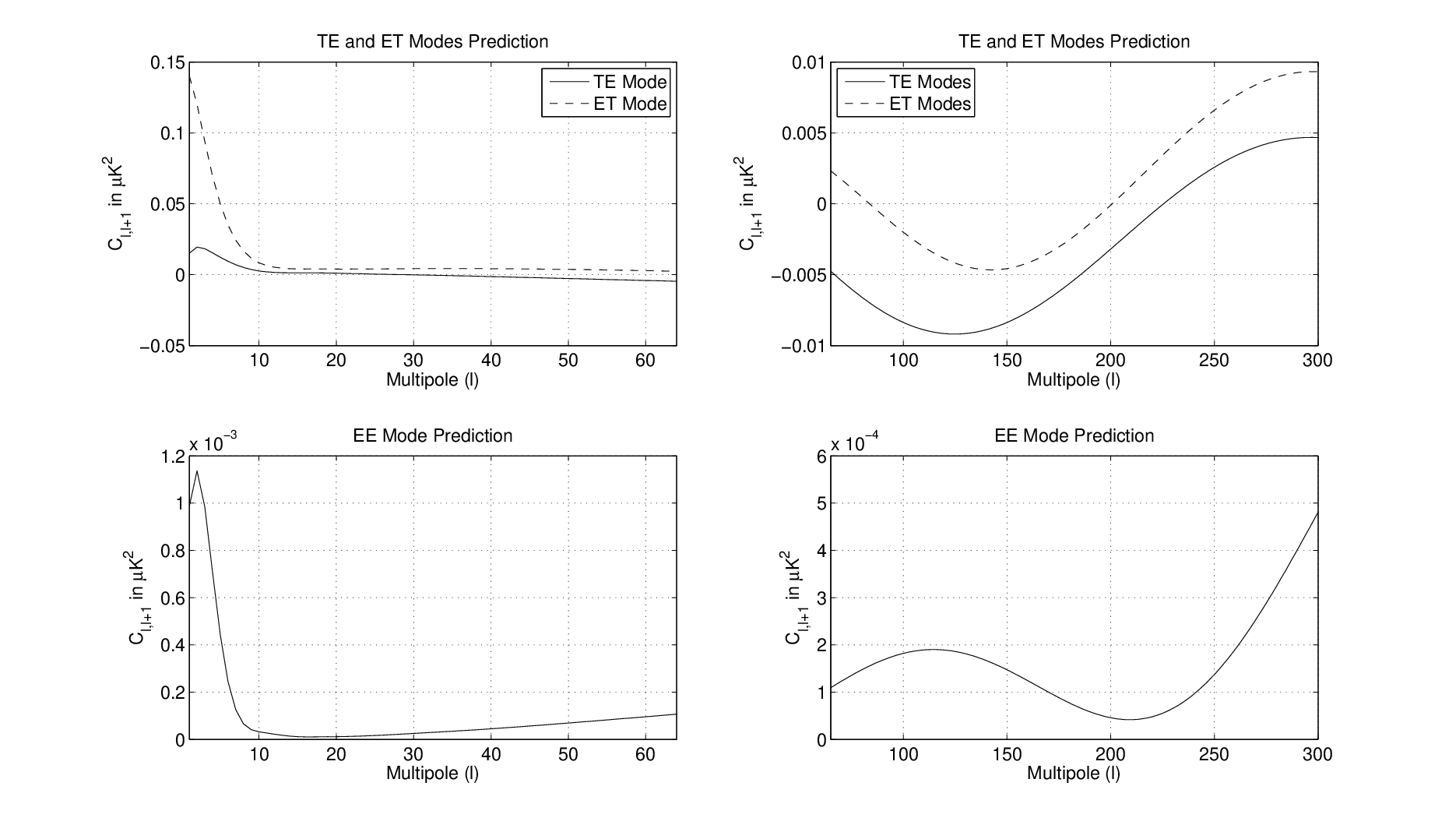
The estimated parameters can be used to predict the signal for the case of polarization data. We use the parameters extracted for the case of the SMICA map in giving our predictions. In this case only data in the three bins, , and is used in determining the model parameters. These provide a somewhat conservative estimate of the dipole modulation. The predictions obtained by using the WILC9 parameters are similar to those obtained by using SMICA. However the amplitude in this case is found to be systematically larger by about 15%. Our results for TT, EE, TE and ET correlations for the case of the inhomogeneous model are shown in Figs. 2 and 3. In Fig. 2 we plot the ratio, defined as,
| (26) |
where is the standard power and is the correlation between and multipoles, defined in Eq. 23. In Fig. 3 we show the predicted value of for TE, ET and EE modes for the inhomogeneous model. The corresponding values for the anisotropic model are shown in Figs. 4 and 5. We find that the ratio for the TT mode is approximately equal to 0.015 at and decays for larger values of . This is true for both the models. The ratio for the EE correlations follow the TT mode closely. The results for the case of are shown in the left panels in these figures whereas those for larger values are shown in the right panels. Since the three bin fit may not be reliable over the larger range of values the results for may be treated as qualitative estimates. However the results for are quantitatively reliable and may be compared with data in order to determine the validity of the inhomogeneous or anisotropic model.
| No of Bins | Maps | Model | |||||
| 3 | WILC9 | Inhomogeneous | |||||
| 3 | WILC9 | Anisotropic | |||||
| 3 | SMICA | Inhomogeneous | |||||
| 3 | SMICA | Anisotropic | |||||
| 6 | WILC9 | Inhomogeneous | |||||
| 6 | WILC9 | Anisotropic | |||||
We give predictions separately for the TE and ET correlations since we find that,
| (27) |
The difference between the two arises due to contributions from the inhomogeneous or anisotropic terms and can be easily extracted from Eq. 13. This difference is particularly interesting in the neighbourhood of where the power of the mode crosses zero. Due to this zero in the denominator, the ratio tends to be very large in the neighbourhood of such points. We find that for the inhomogeneous model, the mode remains positive whereas the mode becomes negative for . Hence the ratio for the mode is positive (negative) for (). The ET mode shows the opposite trend in the neighbourhood of . This appears to be a rather interesting signature of the inhomogeneous model which should be testable with the polarization data. Furthermore the anisotropic model (Fig 4) shows a more pronounced trend which is opposite to what is seen for the case of inhomogeneous model. In this case it is the ratio of the ET mode which stays positive for and becomes negative for with the TE mode showing the opposite trend. Hence we find a qualitatively different behaviour for these two models which might be useful in order to distinguish between them.


5 Conclusion
We have investigated the implications of the hemispherical power anisotropy within the framework of an inhomogeneous and independently an anisotropic Universe model. The Universe is assumed to be inhomogeneous and/or anisotropic at very early pre-inflationary times. This produces a modification of the primordial power spectrum which is parametrized in terms of a simple index and amplitude of the inhomogeneous or the anisotropic term by making a fit to the observed data. The resulting parameters are used to make predictions for the polarization data, i.e. EE, TE and ET correlations between multipoles corresponding to and .
In our analysis we mostly emphasize the results for for which the contribution due to detector noise is negligible. For the case of WMAP data, however, we also extend our study to larger values including the contribution due to detector noise. We find that the signal of dipole modulation is smaller for in comparison to the lower values. We use the theoretical parameters extracted by fitting data for the three bins corresponding to for the case of SMICA map in showing our predictions. We find that the results for the case of WILC9 map are very similar. However the amplitude in this case is found to higher by about 15% in comparison to that found in the case of the SMICA map. We separately show our predictions for and for larger values. For our predictions are quantitatively reliable whereas for larger values they should be treated as qualitative estimates.
We show the results for the ratio of (which is the correlation between and multipoles) to the power . We find that the results for EE mode follow the TT mode closely. The ratio is found to be roughly around 0.02 for and decays for larger values. We find that the results for the TE mode differ from those of ET mode. The difference is emphasized in the inequality shown in Eq. 27. For larger values, in the neighbourhood of , the two modes show qualitatively different behaviour which may provide a very clean signature of these primordial models. These predictions can be tested in the new data available from PLANCK. Alternatively it may provide stringent constraints on these models.
Acknowledgments
Rahul Kothari sincerely acknowledges CSIR, New Delhi for the award of fellowship during the work. Some of the results in this paper have been derived using HealPix package (Gorski, 2005). We used standard Boltzmann solver CAMB (http://camb.info/readme.html) for our theoretical calculations. Finally, we acknowledge the use of PLANCK data available from NASA LAMBDA site (http://lambda.gsfc.nasa.gov).
References
- Ackerman et al. (2007) Ackerman L., Carroll S. M., Wise M. B., 2007, Phys. Rev. D, 75, 083502
- Ade et al. (2014a) Ade P. A. R., et al., 2014a, Astron. Astrophys. 571, A23, [arXiv:1303.5083]
- Ade et al. (2014b) Ade P. A. R. et al., 2014b, Astron. Astrophys. 571, A16, [arXiv:1303.5076]
- Akofor et al. (2008) Akofor E., Balachandran A. P., Jo S. G., Joseph A. and Qureshi B. A., 2008, JHEP, 0805, 092
- Akofor et al. (2009) Akofor E., Balachandran A. P., Joseph A., Pekowsky L. and Qureshi B. A., 2009, Phys. Rev. D, 79, 063004
- Akrami et al. (2014) Akrami Y. et al., 2014, ApJL, 784, L42
- Aluri (2012) Aluri P. K. and Jain P., 2012, Mod. Phys. Lett. A, 27, 1250014
- Bennett et al. (2011) Bennett C. L. et al., 2011, ApJS, 192, 17
- Bennett (2013) Bennett C. L. et al., 2013, Astrophys. J. Suppl. Ser. 208, 20
- Berera et al. (2004) Berera A., Buniy R. V. and Kephart T. W., 2004, JCAP, 10, 016
- Boehmer and Mota (2008) Boehmer C. G. and Mota D. F., 2008, Phys. Lett. B, 663, 168
- Bridges et al. (2007) Bridges M. et al., 2007, MNRAS, 377, 1473
- Cai et al. (2013) Cai Y. F., Zhao W. and Zhang Y., 2013, Phys. Rev. D, 89, 023005
- Campanelli et al. (2007) Campanelli L., Cea P. and Tedesco L., 2007, Phys. Rev. D, 76, 063007
- Carroll et al. (2010) Carroll S. M., Tseng C. Y. and Wise M. B., 2010, Phys. Rev. D, 81, 083501
- Chang & Wang (2013a) Chang Z. and Wang S., 2013a, Eur. Phys. Jour. C, 73, 2516
- Chang et al. (2013) Chang Z., Li X. and Wang S., 2013b, [arXiv:1307.4542]
- Chang & Wang (2013b) Chang Z. and Wang S., 2013b, [arXiv:1312.6575]
- Donoghue & Donoghue (2005) Donoghue E. P. and Donoghue J. F., 2005, Phys. Rev. D, 71, 043002
- Erickcek et al. (2008) Erickcek A. L., Kamionkowski M., and Carroll S. M., 2008, Phys. Rev. D., 78, 123520
- Eriksen et al. (2004) Eriksen H. K. et al., 2004, ApJ, 605, 14
- Eriksen et al. (2007) Eriksen H. K. et al., 2007, ApJL, 660, L81
- Ghosh et al. (2007) Ghosh T., Hajian A. and Souradeep T., 2007, Phys. Rev. D, 75, 083007
- Ghosh (2014) Ghosh S., 2014, Phys. Rev. D, 89, 063518
- Gordon et al. (2005) Gordon C. et al., 2005, Phys. Rev. D, 72, 103002
- Gordon et al. (2007) Gordon C., ApJ, 2007, 656, 636
- Gorski (2005) Gorski K. et al., 2005, ApJ, 622, 759
- Groeneboom et al. (2011) Groeneboom N. E., Axelsson M., Mota D. F. and Koivisto T. S., 2011, arXiv:1011.5353.
- Hanson & Lewis (2009) Hanson D. and Lewis A., 2009, Phys. Rev. D, 80, 063004
- Hansen et al. (2009) Hansen F. K. et al., 2009, ApJ, 704, 1448
- Hoftuft et al. (2009) Hoftuft J. et al., 2009, ApJ, 699, 985
- Jaffe et al. (2006) Jaffe T. R. et al., 2006, ApJ 644, 701
- Jain & Rath (2014) Jain P. and Rath P. K., 2014, Eur. Phys. J. C, 75, 3, 113, [arXiv:1407.1714]
- Kahniashvili et al. (2008) Kahniashvili T., Lavrelashvili G. and Ratra B., 2008, Phys. Rev. D, 78, 063012
- Koivisto & Mota (2011) Koivisto T. S. and Mota D. F., 2011, JHEP, 1102, 061, arXiv:1011.2126
- Koivisto & Mota (2006) Koivisto T. and Mota D. F., 2006, Phys. Rev. D, 73, 083502
- Koivisto & Mota (2008) Koivisto T. and Mota D. F., 2008, JCAP, 08, 021
- Kothari et al. (2015) Kothari R., Rath P. K. and Jain P., 2015, arXiv:1503.03859.
- Land & Magueijo (2006) Land K. and Magueijo J., 2006, MNRAS, 367, 1714
- Lewis (2000) Lewis A. et al., 2000, ApJ 538, 473-476
- Liu et al. (2013) Liu Z. G., Guo Z. K. and Piao Y. S., 2013, Phys. Rev. D, 88, 063539
- Mcdonald (2014) McDonald J., 2014, Phys. Rev. D 89, 127303 [arXiv:1403.2076]
- Mazumdar & Wang (2013) Mazumdar A. and Wang L., 2013, JCAP, 10, 049
- Namjoo (2014) Namjoo M. H. et al., 2014, [arXiv:1411.5312]
- Paci et al. (2013) Paci F. et al., 2013, MNRAS, 434, 3071
- Prunet et al. (2005) Prunet S. et al., 2005, Phys. Rev. D, 71, 083508
- Pontezen & Challinor (2007) Pontzen A. and Challinor A., 2007, MNRAS, 380, 1387
- Rath et al. (2013a) Rath P. K. et al., 2013a, JCAP, 04, 007
- Rath & Jain (2013) Rath P. K. and Jain P., 2013, JCAP, 12, 014
- Rath et al. (2014) Rath P. K., Aluri P. K. and Jain P., 2014, Phys. Rev. D, 91, 2, 023515, [arXiv:1403.2567]
- Schmidt & Hui (2013) Schmidt F. and Hui L., 2013, Phys. Rev. Lett. 110, 011301
- Wang & Mazumdar (2013) Wang L. and Mazumdar A., 2013, Phys. Rev. D, 88, 023512
- Watanabe et al. (2010) Watanabe M., Kanno S. and Soda J., 2010, Prog. Theo. Phys. 123, 1041
- Wald (1983) Wald R. M., 1983, Phys. Rev. D, 28, 8, p.2118
- Zaldarriaga & Seljak (1997) Zaldarriaga M. and Seljak U. , 1997, Phys. Rev. D, 55, 1830
- Zarei (2014) Zarei M., 2014, [arXiv:1412.0289]