Identification of galaxy cluster substructures with the Caustic method
Abstract
We investigate the power of the caustic technique for identifying substructures of galaxy clusters from optical redshift data alone. The caustic technique is designed to estimate the mass profile of galaxy clusters to radii well beyond the virial radius, where dynamical equilibrium does not hold. Two by-products of this technique are the identification of the cluster members and the identification of the cluster substructures. We test the caustic technique as a substructure detector on two samples of 150 mock redshift surveys of clusters; the clusters are extracted from a large cosmological -body simulation of a CDM model and have masses of and in the two samples. We limit our analysis to substructures identified in the simulation with masses larger than . With mock redshift surveys with 200 galaxies within , (1) the caustic technique recovers % of the real substructures, and (2) % of the substructures identified by the caustic technique correspond to real substructures of the central cluster, the remaining fraction being low-mass substructures, groups or substructures of clusters in the surrounding region, or chance alignments of unrelated galaxies. These encouraging results show that the caustic technique is a promising approach for investigating the complex dynamics of galaxy clusters.
Subject headings
galaxies: clusters: general, (cosmology:) large-scale structure of universe, methods: N-body simulationsI. Introduction
Galaxy clusters, as the high-mass tail of the hierarchical structure, connect the large-scale structure to galaxies, and are thus relevant for constraining models of galaxy evolution, structure formation, and cosmology. Due to the large scale and long relaxing time of clusters, the presence of substructures is quite common, indicating that a number of clusters are likely to be out of equilibrium. Substructures can substantially affect the estimate of the cluster velocity dispersion and mass [35, 65], can provide insights into the formation process of the cluster, and unveil the existence of dark matter [53, 11]. The presence of substructures appears to be a fundamental ingredient of the galaxy-environment connection and for shaping the morphology-density relation [26, 36, e.g.,]. The mass fraction in substructures can also probe structure formation and the expansion rate of the universe [70, 43, 56, 85].
Attempts to identify and investigate cluster substructures have been numerous since their first discovery in the optical band [80]. In images of X-ray surface brightness, substructures are relatively obvious, especially with data coming from recent X-ray missions, including ROSAT [46, 76], Chandra[41, 4, 61], and XMM-Newton[91].
However, because the X-ray surface brightness decreases rapidly with increasing radius, these observations can only trace substructures in the central region of clusters. Substructures can also appear in microwave observations because free electrons in the hot X-ray gas originate the Sunyaev-Zeldovich effect [47, 48]. The location of radio halos in clusters also tends to coincide with the substructures observed in X-ray images and temperature maps [see 27, for a recent review].
The existence of substructures in the dark matter halos of clusters can also be revealed by the anomalous images of strong gravitational lensing systems [45, 52, 51], or by peculiar features of the halo density profiles of weak lensing systems [38, 11, 59, 63, 58, 54, 81], although the contamination by chance alignments of unrelated massive systems along the line of sight can be severe [37, 39, 31].
The detection of substructures from optical data, based on the galaxy celestial coordinates and redshifts, is still a common approach for studying substructures. The methods can either use galaxy positions alone, redshifts alone, or both.
The methods that use galaxy positions alone include the smoothed density-contour maps [30], symmetry test, angular separations test, density contrast test [89], average two-point correlation function [74], and two-dimensional (2D) wavelet transforms [82, 24, 28]. They usually suffer from the contamination of background and foreground galaxies, but are clearly very useful when spectroscopic observations are missing or incomplete.
The methods that only use the galaxies’ redshifts usually assume that the distribution of the velocities of the member galaxies is Gaussian. Based on this assumption, the indicators like kurtosis, skewness [88, 83], and the asymmetry and tail indices [10] are designed to quantify the subclustering in the one-dimensional (1D) redshift distribution. The 1D Kaye’s mixture model (KMM) algorithm belongs to the set of Gaussian mixture model (GMM) methods: it assesses the presence of substructures by estimating the number of optimal partitions of Gaussian distributions [5, 49]. The DEDICA method is based on an adaptive kernel and identifies specific velocity components [66]; when the chosen kernel is Gaussian, DEDICA reduces to one of the GMM methods.
Among the methods using both the galaxy positions and redshifts, the Dressler & Shectman (DS) method [23, 83, 44, 2, 22] is certainly the most widely used. Other methods include the three-dimensional (3D) KMM algorithm [9, 13, 8], which, in input, requires the number of the substructures and an initial guess of their positions; the 3D wavelet transforms [25, 29, 34, 60]; the 3D version of DEDICA [67, 68]; and the hierarchical tree algorithm [77, 1].
All of these methods mainly focus on the substructure detection. However, an unambiguous association of galaxies to individual substructures, which enables the derivation of the substructure properties, like size, velocity dispersion, and mass, is not yet available. Here we explore the possibility that the caustic technique can contribute a step forward in this direction.
The caustic technique [19, 17, 18] estimates the escape velocity of cluster galaxies from the cluster center to a few times the virial radius. The technique name derives from the two curves in the redshift diagram where the galaxy number density is expected to be infinite in the spherical collapse model [69]. With this technique, we can estimate the mass and gravitational potential profiles of galaxy clusters to radii that extend to the cluster infall region [18, 79, see reviews in]. For the mass estimation, the caustic technique only assumes spherical symmetry and does not require the system to be in dynamical equilibrium. It can be used both in the central and in the outer regions of clusters, where other techniques cannot be applied.
The first step of the caustic technique procedure is to arrange the galaxies in a binary tree according to a projected pairwise galaxy binding energy. This step is similar to the procedure described in Serna & Gerbal [77]. However, the caustic technique goes further and identifies a threshold that cuts the tree and identifies the cluster members. Serra & Diaferio [78] showed that this approach, combined with the location of the caustics in the cluster redshift diagram, returns a list of cluster members within that is 96% complete and only 2% of the members are actually interlopers. Within the larger radius , where no other method is available, the completeness is 95% and the contamination is 8%.
The same principle used to cut the binary tree and identify the cluster members provides a second threshold that gives a list of cluster substructures. So far, no systematic analysis of the properties of these substructures has been performed. Here, we use -body simulations to investigate the power of the caustic technique to identify cluster substructures.
II. The Simulated Cluster Samples
We use the Coupled Dark Energy Cosmological Simulations [7]. This is the largest set to date of -body simulations that model the interaction between the dark energy scalar field and the Cold Dark Matter (CDM) fluid. Here, however, we only consider the simulation of the standard CDM model with fiducial WMAP7 parameters. The simulated volume is a comoving cube of 1 Gpc on a side ( km s-1 Mpc-1 is the dimensionless Hubble constant), containing CDM particles with a mass of and the same number of baryonic particles with a mass of . We only consider the dark matter particles: we assume that in the real universe galaxies are unbiased tracers of the velocity field of the dark matter particles. In fact, both -body simulations [20, 21, 33, 32, e.g.,] and observations [72, e.g.,] indicate that any velocity bias between galaxies and dark matter is smaller than 10%.
Halos are identified with the Friends-of-Friends (FoF) algorithm [40, 16], which links particles with distances less than the linking length to form a group. We adopt the standard linking length , with as the mean interparticle separation, corresponding to the overdensity at viralization [6], with as the mean background density. In this procedure, the FoF halos are identified by using the CDM particles as primary tracers and then linking baryonic particles to the group of their closest CDM neighbor. The characteristic radius of the FoF halos, , is the radius within which the average density (including both CDM and baryonic particles) is 200 times the critical density. The mass within is .
We consider two samples of 50 FoF halos, each at redshift : a massive sample (M15 hereafter), with ranging from to , and median ; and a less massive sample (M14 hereafter), with masses ranging from to , and median .
For each cluster, we compile three mock galaxy redshift catalogs. Each cluster is located at the center of the volume using the periodic boundary conditions of the simulation box. We assign the celestial coordinates and a redshift distance km s-1 to the cluster center. Around the cluster, we consider a rectangular prism enclosing the volume, corresponding to a solid angle that at the cluster distance covers a square area Mpc wide. The volume is centered at the cluster and it is Mpc deep. The resulting field of view (FOV) is . For each cluster, we apply this procedure to three orthogonal directions. Since the clusters are generally not spherically symmetric, for our statistical purposes we can consider these three mock catalogs as independent clusters. We thus obtain 150 mock redshift catalogs for each of the samples (M15 and M14).
The observational volumes we extract from the simulation typically contain particles for the M15 sample and particles for the M14 sample. Realistic numbers of observable galaxies in these volumes are clearly much smaller. Therefore, we randomly sample the dark matter particles until we obtain a given number of particles within . To explore the effect of galaxy sampling, we build catalogs with (100, 200, 300, 400, and 500). Additionally, we only retain particles within km s-1 from the cluster center. These mock galaxy redshift surveys of cluster regions are roughly comparable to recent large surveys of clusters and their surroundings, such as CIRS [71] and HeCS [73].
A different strategy to build mock redshift surveys could be to keep the number of particles in the FOV for both the M14 and M15 samples fixed. However, this procedure returns mock surveys where the substructures of the M14 clusters are poorly sampled or, more often, not sampled at all, because as mentioned above the observational volumes of the M14 sample are on average 60% () less populated than the M15 sample volumes. On the contrary, keeping fixed guarantees that we properly sample the substructures and guarantees that it is closer to the observational procedure of surveys dedicated to the study of the dynamics of clusters; these surveys tend to sample the volume more densely around the cluster, both on the sky and in redshift space. The very different final numbers of particles in the FOV of the M14 and M15 samples (Table 1) reflects a real effect: identifying substructures in less massive clusters requires denser surveys because in these clusters the probability of measuring the redshift of a galaxy that does not belong to the cluster is larger.
For a given , the total numbers of particles in the FOV of a mock cluster depend on the cluster and its surrounding region. To investigate the effects of the fluctuations caused by random sampling, we repeat the procedure 10 times. Table 1 lists the medians and percentile ranges of the number of particles as a function of : for example, 80% of the mock catalogs of the M15 sample with have in the range of . For our statistical purposes, these 10 random realizations of each individual line-of-sight projection of a given cluster with a fixed cannot be considered independent. Hereafter, we will only use these 10 realizations to quantify the fluctuations of the random sampling on the cluster samples M15 and M14. Finally, in the M14 FOV’s is four to five times larger than in the M15 samples: because the M15 clusters are an order of magnitude more massive than the M14 clusters, whereas the surrounding cosmic volumes are comparable, in the M15 samples the random sampling reaches more rapidly and the number of particles sampled in the surrounding region is proportionally smaller.
| M15 (1500 clusters) | M14 (1500 clusters) | |||||
| 10% | 50% | 90% | 10% | 50% | 90% | |
| 100 | 185 | 241 | 325 | 672 | 996 | 1490 |
| 200 | 369 | 481 | 644 | 1356 | 2014 | 2905 |
| 300 | 553 | 718 | 969 | 2034 | 2988 | 4385 |
| 400 | 739 | 962 | 1283 | 2704 | 4016 | 5829 |
| 500 | 923 | 1195 | 1603 | 3394 | 5034 | 7258 |
To identify the substructures of the clusters in the simulations, we use the code SUBFIND [84], whose algorithm is based on the overdensity and the gravitational binding energy of the particles. More specifically, for each FoF halo detected by the FoF algorithm, SUBFIND identifies candidate substructures by sorting the particles of the FoF halo according to their local density and isolating local density maxima. This procedure provides substructures whose boundaries are determined by the first saddle point identified in the local density field around each density maximum. From each substructure, we finally remove all particles with positive total energy [see 7, for further details].
The mass of a substructure is always its total mass, namely the sum of the mass of the particles (both CDM and baryons) that are gravitationally bound to that substructure as identified by SUBFIND. The first row of Table 2 lists the total number of substructures with masses larger than in our two samples M15 and M14. The mass threshold is not arbitrary, but is a minimum substructure mass set by the number of luminous galaxies that can be detected in current typical surveys. In fact, a substructure is expected to contain at most a handful of galaxies brighter than . Hereafter, we will call these substructures 3D substructures.
By randomly sampling the dark matter particles, the number of members of a 3D substructure in the mock catalog can be substantially reduced or even vanish. We only consider 3D substructures that have at least 10 particles appearing in the FOV.
Table 2 lists the total number of clusters with at least one 3D substructure appearing in the FOV, the total number of 3D substructures in all the FOVs , and the ratio between these detectable substructures and the total number of substructures (); the total number of substructures is listed in the first row of Table 2. As expected, the number of 3D substructures appearing in the FOV increases with increasing . We also list the standard deviations deriving from the ten random realizations. We see that the random sampling has a moderate impact. In the M15 samples, the number of clusters that do not show 3D substructures in the FOV is substantial: if we consider the total members of the cluster as the sum of the members of the 3D substructures and the members of the cluster core identified by SUBFIND, % of the total members belong to the 3D substructures in the M14 samples, whereas this fraction is only % in the M15 samples. In addition, as mentioned earlier, the M15 FOV’s are 4 to 5 times less populated than the M14 fields. Therefore, random sampling makes 3D substructures in the M15 samples vanish more easily than in the M14 samples.
| M15 | M14 | |||||
|---|---|---|---|---|---|---|
| Ratio(%) | Ratio(%) | |||||
| - | 150 | 594 aafootnotemark: | - | 150 | 282 aafootnotemark: | - |
| 100 | 15 1 | 15 2 | 2.5 | 146 1 | 191 2 | 67.7 |
| 200 | 39 3 | 40 3 | 6.7 | 150 1 | 254 4 | 90.1 |
| 300 | 61 4 | 64 4 | 10.8 | 150 0 | 275 3 | 97.5 |
| 400 | 81 4 | 94 5 | 15.8 | 150 0 | 282 1 | 100 |
| 500 | 99 3 | 132 6 | 22.2 | 150 0 | 282 0 | 100 |
III. The Caustic Method
According to hierarchical clustering models, clusters of galaxies form by the aggregation of smaller systems. The local gravitational potential plays a crucial role in determining the galaxy velocities in addition to the radial infall expected in the spherical collapse model [19]. On the redshift diagram of the line-of-sight velocity of the galaxies in the cluster rest frame versus their projected distance from the cluster center, the cluster members populate a trumpet-shaped region that is approximately symmetric around the axis [42, 69, 87]. The caustics define the boundaries of this region, whose amplitude decreases with increasing . provides the estimate of the escape velocity profile from the cluster and thus its mass profile [19, 17].
To measure , the caustic technique builds a binary tree based on the projected galaxy pairwise energy, determines a threshold to cut the binary tree, identifies a set of candidate cluster members that in turn determines the cluster center and defines the redshift diagram. The caustic technique locates the caustics and thus from the galaxy number density on the redshift diagram. The steps that are relevant for the identification of the substructures we are interested in here are the construction of the binary tree and its threshold determination. For the sake of completeness, we list the details of these steps. Further details are provided in Diaferio [17] and Serra et al. [79].
To build the binary tree, we proceed as follows:
- i.
initially each galaxy is a group ;
- ii.
the binding energy , where is a projected binding energy between the galaxy and the galaxy , is associated to each group pair . The projected binding energy is estimated with the relation
(1) where is the pair projected separation, is the line-of-sight velocity difference and M⊙ is the typical total mass of a luminous galaxy;
- iii.
the two groups with the smallest binding energy are replaced with a single group and the total number of groups is decreased by one;
- iv.
the procedure is repeated from step (ii) until only one group is left.

At this stage all the galaxies are arranged in a binary tree; an example is shown in Figure 1. This dendrogram is derived from a mock catalog of the M14 sample with and . To identify the cluster members and its substructures, we need to cut the tree at some level. Toward this aim, we identify the main branch from the root to the leaves by tracing the node that contains the largest number of galaxies at each bifurcation. The leaves that hang from each node of the main branch provide a velocity dispersion . When walking along the main branch from the root to the leaves, rapidly decreases due to the progressive loss of galaxies that are most likely not associated with the cluster (Figure 2); then reaches a “ plateau” at some node . Most of the galaxies hanging from this node are members of the cluster: in fact, the system is nearly isothermal and moving along the main branch toward the leaves removes the less bound galaxies that in general do not substantially affect the value of . When we get close to the leaves along the main branch, the remaining galaxies have a binding energy that is very small and causes to drop again. This second rapid drop identifies the node that sets the limit of the plateau.
To identify the plateau and its boundaries and , Serra et al. [79] designed an algorithm based on the distribution of the velocity dispersions of the nodes, as detailed below.
- i.
Derive the probability density distribution of the velocity dispersion of the leaves hanging from each node; an example is shown in the right panel of Figure 2. The mode of this distribution corresponds to the value of the plateau.
- ii.
To identify the nodes belonging to the plateau, (1) we remove the tails beyond of the distribution, and (2) the 80% of the remaining nodes closest to are retained as the nodes defining the plateau.
- iii.
We choose among the first (i.e., closest to the root) five nodes of the set of the nodes, as the node whose has the smallest discrepancy from ; similarly we choose among the last five nodes (i.e., furthest away from the root).
The first node, , closest to the root, is the appropriate level for the identification of the cluster. The threshold set by node separates the binary tree branches into different groups. The group containing the main branch is the main group and its galaxies are the candidate members of the cluster. The completeness and purity of these candidate members have been investigated by Serra & Diaferio [78]. We consider all of the other groups separated by the threshold dynamically distinct from the cluster, or the main group, and we disregard them hereafter.
The second node, , farthest away from the root, identifies the substructure candidates. We define all the substructures, whose members belong to the main group, as the 2D substructures of the cluster. We only consider 2D substructures with at least 10 particles. We disregard all of the systems separated by the threshold set by node whose members do not belong to the main group. As an example, Figure 3 shows the distribution on the sky of the identified groups and the 2D substructures according to the dendrogram and plateau of Figures 1 and 2.


the same as in Figure 1.
IV. Analysis and Results
IV.1. Cluster identification
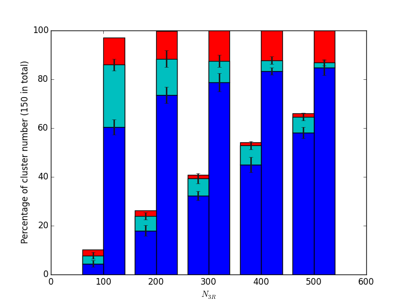
Because of the random sampling of particles, some substructures might have less than ten particles in the FOV. According to our limit, these substructures are not taken into account. If all the 3D substructures vanish from the field of view, the cluster has no substructures left. The height of the bars of each bin in Figure 4 shows the total fraction of clusters that have 3D substructures in the FOV. These fractions correspond to the number of clusters listed in Table 2. As noted in the previous section, almost all of the clusters in the M14 samples show 3D substructures, whereas many clusters of the M15 samples have had all of their 3D substructures disappear.
When constructing the binary tree from the data set of a cluster redshift survey, the main group of the binary tree might identify a system different from the cluster we are interested in because this cluster might not be the richest system in the FOV. With real data sets, where we usually analyze the clusters individually, we can easily correct for this situation by reducing the area of the FOV or by imposing the desired cluster center. Here, where we analyze large samples of mock clusters automatically and blindly, we simply remove these cases. To check whether the main group identifies the correct cluster, we compare the 2D members, namely the members of the main group, with the 3D members of the cluster core identified by SUBFIND. We say that a cluster is correctly identified if at least 60% of its 3D members are in the list of the 2D members. In Figure 4 the sum of the blue and cyan sectors of the bars shows the fraction of correctly identified clusters; the red sectors of the bars show the fraction of misidentified clusters.
The fraction of correctly identified clusters is further split into the fraction of clusters with 2D substructures, shown by the blue sectors, and the fraction of clusters with no 2D substructures, shown by the cyan sectors. The lack of 2D substructures is usually caused by a relatively low second threshold that does not leave a sufficiently large number of particles for the substructure identification.
In passing, we note that we confirm the results of Serra & Diaferio [78], who find that on average in clusters identified by the plateau, 13% of the members within are actually interlopers (see their Table 1, 7th column, 9th row). Therefore, increasing our 60% threshold only slightly decreases the fraction of correctly identified clusters, for example, only by 1% if we increase the threshold to 80%. Substructures are more poorly populated and proportionally more difficult to detect than clusters. As we see below, for substructures, a 60% threshold turns out to be a reasonable compromise between the completeness and the success rate: we thus also use the 60% threshold for the clusters to adopt a single criterion for both structures.
IV.2. 2D versus 3D substructures: The success rate
To quantify whether the 2D substructures correspond to the 3D substructures, we make a one-to-one comparison between the members of the 2D substructures identified by the binary tree and the members of the 3D substructures identified by SUBFIND. A single 2D substructure may contain members belonging to different 3D substructures or none. We find that in all of the M15 and M14 samples combined, 49% of the 2D substructures contain at least one member of a 3D substructure. For each of these 2D substructures, we define as the largest fraction of its total number of members that are also members of a single 3D substructure. Figure 5 shows the distribution of : 51% of the 2D substructures have an larger than 0.8. We adopt , a value smaller than the median , as the threshold to consider a 3D substructure successfully identified by a 2D substructure. Adopting a smaller threshold increases the success rate at the expense of increasing the discrepancy between the properties of the 2D and 3D substructures. A larger threshold makes the identification more solid, but substantially drops the success rate.
It can happen that different 2D substructures contain members of the same 3D substructure. This event occurs for 12% of the 2D substructures of the M14 samples and for 1.2% of the 2D substructures of the M15 samples. In these cases, we take the 2D substructure containing the largest number of the 3D substructure members as the match to the 3D substructure.
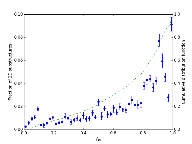
Figure 6 shows a random example of the substructure identification. The cluster has only one 3D substructure, whose center is indicated by the yellow star. The caustic method returns seven 2D substructures in addition to the cluster core, indicated by the yellow square, which is correctly matched. One of the 2D substructures correctly coincides with the 3D substructure. Out of the remaining six 2D substructures that do not correspond to any 3D substructure of the cluster identified with SUBFIND, two are close to the core and four are relatively distant from the cluster center. We consider these six 2D substructures to be false detections.

In fact, in our statistical analysis, we consider as false detections all the 2D substructures that do not correspond to the 3D substructures that SUBFIND associates with the analyzed cluster. However, our choice is rather restrictive. Figure 7 shows the 3D distribution of the system shown in Figure 6: out of the six 2D substructures, only one system is due to chance alignment; the remaining five 2D substructures are clearly bound systems. Two of them, close to the cluster core, are not in our list of 3D substructures because they have masses smaller than . The remaining three 2D substructures are groups surrounding the cluster center. As mentioned above, we do not include them in our list of 3D substructures in order to restrict our analysis to the 3D substructures of the analyzed cluster.
This random example shows that the rate of successful detections and the completeness we will show below are clearly correct in the context of focusing on the massive substructures of individual clusters, but are likely to be lower limits to the performance of the identification of bound systems from redshift data with the caustic technique.

Figures 6 and 7 suggest that the 2D substructures at large projected distances from the cluster center are likely to be groups and substructures of surrounding clusters. We thus compute the success rate, namely the ratio between the number of 2D substructures that correspond to 3D substructures and the total number of 2D substructures, as a function of distance from the cluster center. Figure 8 shows this relation for the combined M14 and M15 samples. The success rate peaks at different radii in the two samples because the clusters have different sizes. When the radii are normalized to , both peaks appear in the range . We keep the length in this plot in proper units, because these units are more convenient with real data; in addition, the mass distribution of each cluster sample is very peaked and the distance normalization plays a little role within the same cluster sample. The success rate shows a broad peak between and Mpc for the M14 samples and between and Mpc for the M15 samples, whereas it decreases at the center and in the outskirts of the clusters. The low rate at small distances is due to the cases where the cluster core is identified as a substructure rather than as the core itself. Again, we consider these cases to be false detections because we are interested in the 3D substructure identification, although these identified 2D substructures actually are bound systems. In the cluster outskirts, the number of 3D substructures clearly decreases, unlike the number of 2D substructures. Therefore, we can introduce a distance criterion by removing all of the 2D substructures at distances outside a given range that, based on Figure 8, we arbitrarily choose to be Mpc: this criterion can remove most of the many false detections without missing promising 2D substructures.
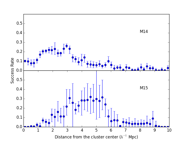
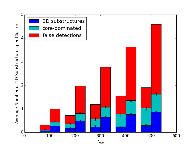
Figure 9 shows the success rate as a function of , with the distance criterion applied. The average number of 2D substructures increases with , as expected, whereas the success rate decreases from 25% at to 15% at (these fractions can be read off in Figure 9 from the ratio between the length of the blue sector of each bar and the total length of the bar): In fact, a larger number of particles in the FOV increases the sampling of the 3D substructures, but at the same time it increases the probability of detecting 2D substructures by chance alignment. The cyan sectors of the bars show the fraction of 2D substructures whose members are 3D members of the cluster core rather than members of the 3D substructures. The error bars show that the random sampling fluctuations have a small impact.
We can look at our results from a different perspective. Figure 10 shows the distribution of the success rate. The y- and x-axes show and the success rate, respectively. The gray scale shows the fraction of clusters on this plane. For example, the bottom row of the bottom panel shows that 63% of the clusters in the M15 sample with have no successful detection, whereas in 34% of the clusters all the 2D substructures correspond to real 3D substructures.
This figure clearly shows that clusters are not uniformly distributed on this plane. In fact, the number of 2D substructures is discrete and may be small, with just one or two 2D substructures, especially when is small. Figure 10 also shows that in all of the M15 samples, about 60% of the clusters have 2D substructures that are false. This result is due to the fact that there are fewer particles belonging to 3D substructures in the FOV of massive clusters (see Sect. II). The lack of substructures makes the boundary of the plateau quite ambiguous and, consequently the identification of the second threshold becomes more problematic. On the contrary, the success rate in the M14 samples is more equally distributed on the plane and the fraction of false 2D substructures is proportionally smaller.

IV.3. Completeness
We now estimate the completeness of our samples of substructures, namely the ratio between the number of correctly identified 3D substructures and the total number of 3D substructures. We note that the total number of 3D substructures only includes the 3D substructures more massive than and with at least 10 particles in the FOV.

The completeness of the individual samples is shown in Figure 11. The completeness increases with from 18% to 29% for the M15 samples, and from 34% to 60% for the M14 samples. As for Figure 9, these fractions can be read off in Figure 11 from the ratio between the length of the blue sector of each bar and the total length of the bar.
Figure 12 shows the completeness as a function of the substructure mass for the M14 samples. Clearly, the most massive substructures are detected more easily, and more substructures are recognized in denser fields. The largest 3D substructure mass is ; this mass is larger than the maximum of the M14 sample, but it still is a factor of smaller than the minimum total cluster mass , which is defined as the sum of the mass of the dark matter and baryonic particles of the FoF halo, consistently with the computation of the mass of the 3D substructures. Figure 12 shows that we can obviously improve the completeness of our substructure sample by increasing the lower mass limit. The result is qualitatively similar to the results of the M15 samples, which we do not show here, although in this case, the trend has larger fluctuations and discontinuities due to the limited number of clusters and detected substructures.

To illustrate the origin of the relations plotted in Figure 12, we show two examples of the substructure mass function in Figure 13. The red histogram is the original mass function of the 3D substructures in the 150-cluster M14 sample, whereas the blue histogram shows the estimated mass function: the original mass function is not monotonic and is severely under-represented by the estimated mass function at the low-mass end.
This analysis of the dependence of the completeness on the minimum mass of the 3D substructure unfortunately cannot be repeated with the success rate. In fact, the substructure mass does not enter our algorithm for the identification of substructures from redshift data: changing the mass threshold would only change the number of 3D substructures, but it would leave the number of 2D substructures unaltered. Therefore, if we increase the mass threshold, the success rate simply decreases; if we decrease the mass threshold below , we start probing substructures with one or two bright galaxies at most, namely substructures that are virtually impossible to detect with current redshift surveys.
V. Discussion
V.1. Possible developments of the caustic technique
In the previous sections we show that the caustic technique, when blindly applied to redshift surveys of clusters, provides encouraging values of the success rate and completeness. In principle, these results could be improved when a cluster is analyzed individually. In fact, the assumption that the two nodes, and , and their corresponding thresholds alone are sufficient to separate the groups surrounding the cluster as well as the cluster substructures might be too simplistic in some clusters: their dynamical state can be complex enough that the deviation from the single isothermal sphere is relevant. In this case, looking for a single plateau on the main branch might fail to capture the full information on the cluster dynamics contained in the binary tree.
For example, the velocity dispersion of the main group can substantially differ from the velocity dispersion of the substructures, and in turn different substructures can have different velocity dispersions. This situation can generate multiple plateaus on the main branch and the determination of the proper thresholds is ambiguous. In these cases, the algorithm might not identify the main group and its substructures satisfactorily and might miss a substantial number of 3D substructures with velocity dispersions smaller than the velocity dispersions set by the plateau.
Figure 14 illustrates this argument: it shows the distributions of the velocity dispersions of the 3D cores (green histograms), 3D substructures (red histograms), and the 2D substructures corresponding to 3D substructures (identified 3D substructures, blue histograms) for all of the combined M14 and M15 samples. The velocity dispersions of the 3D cores and substructures are computed with the full list of members provided by SUBFIND, whereas the velocity dispersion of the identified 3D substructures are computed from the list of members derived from the binary tree. In the M14 samples, the velocity dispersions of the cores and of the 3D substructures substantially overlap. Therefore the velocity dispersion corresponding to the single plateau of the main branch of the binary tree can properly identify both the main group and the substructures. On the contrary, in the M15 samples, the distributions of the velocity dispersions of the cores and of the 3D substructures are almost completely separated and the plateau that identifies the main branch is unlikely to alo properly identify the substructures. Figure 14 thus suggests that this is the origin of most of the differences between the substructure identification results of the M14 and M15 samples that we describe in the previous sections.
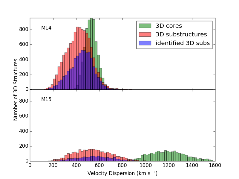
In conclusion, the closer the velocity dispersions of the 3D substructures are to the velocity dispersion of their cores, namely to the plateau, the more effectively our algorithm detects the 3D substructures. When applied to clusters individually, as it can happen with real catalogs containing fewer clusters, if the shape of the velocity dispersion on the main branch vs. the node number (Figure 2) is more complex than a single plateau, the substructure detection can be improved by tuning the substructure threshold according to this shape. We plan to investigate this issue in detail in future work.
As a final note, we emphasize that our analysis is based on the assumption that a set of dark matter particles randomly sampled from an -body simulation is a fair representation of a real sample of galaxies. This assumption is expected to be valid at the high-mass end of the dark matter halo mass function, but it can become progressively incorrect at decreasing masses [75]. Therefore, luminosity and velocity segregations can partly differentiate the phase-space distributions of galaxies from those of an unbiased sample of dark matter particles. Associating methods, like the abundance matching technique [14, 86, SHAM;], which assumes a monotonic relationship between observed galaxy luminosity and simulated halo mass, can be used to make tests on mock catalogs that resemble real data sets more closely. In future work we will explore this issue: we expect it to be particularly relevant in dealing with the different sizes of the M15 and M14 mock surveys (Table 1) and in addressing the dependence of the success rate on (Figure 9) in a more realistic context.
V.2. Our results in the context of previous work
Assessing the presence of substructures in clusters has been frequently investigated in the literature based on X-ray observations, weak gravitational lensing, or spectroscopic redshifts of galaxies. However, the issue has been addressed at very different levels.
X-ray analyses mainly focus on quantifying the surface brightness morphology, with the aim of either separating relaxed clusters from merging clusters [62, e.g.,] or quantifying the systematic errors affecting cluster mass measurements [57, 64]. The substructure identification is limited to the cluster central region within , which is the typical largest distance where the ICM can be detected reliably [64], and to substructures that contain a quantity of hot gas large enough to produce a detectable X-ray emission. In addition, the identification of substructures is complicated by the fact that viscosity and magnetic fields can displace the hot gas from the dominant mass distribution, as indicated by the observations of numerous merging clusters [53, 50, 55, e.g.,].
The mass distribution is expected to be directly detected, with studies based on weak gravitational lensing, whose signal is not affected by the complications of baryonic physics and the dynamical state of the cluster. However, unrelated large-scale structures along the line of sight [37, 39] and uncertainties on the lens parametrization [12, 15] can be the sources of substantial systematic errors. For example, when weak lensing is applied to the identification of clusters in -body simulations, projection effects limit the fraction of identified clusters that correspond to real clusters to 20%, whereas the completeness can be as large as 80% [90]. Shirasaki [81] proposes a method based on weak lensing to identify substructures in the outer regions of clusters, beyond 1 arcmin of the cluster center. The method is tested on -body simulations where substructures are identified with SUBFIND. The fraction of real substructures that are identified with this algorithm is never larger than 40%, approximately comparable to our results, whereas the contamination fraction is not mentioned.
The identification of substructures from the galaxy positions and redshifts has a long history, but the various algorithms have rarely been tested on realistic -body simulations. Escalera & Mazure [25] test the wavelet transform method on 12 toy models where the particles of the main cluster are distributed according to a Hubble profile, with a Gaussian distribution of their velocities; only a single substructure, which is a rescaled model of the main cluster, is located away from the cluster core. The wavelet transform method yields a significance level of the identified substructure and Escalera & Mazure [25] show that for two of their significant substructures the fraction of particles that do not actually belong to the 3D substructures is 3/9 and 0/7.
Pinkney et al. [65] investigate 31 different methods, including the DS and the KMM algorithms; only 5 out of these 31 methods use both galaxy redshifts and celestial coordinates. They build two-component merging clusters with -body simulations and apply the methods at different epochs of the merging process and from different lines of sight. Therefore, the resulting mock fields of view contained a single substructure and no foreground and background large-scale structures or field particles. The main goal of their test is to check the efficiency of the substructure identification and the significance level of the detection. The DS method has the best performance, with a success rate of 66% atz 5% significant level, with a false detection rate of 10% in an isolated isothermal cluster. The success rate of the KMM algorithm is around 36%, while the false detection rate rapidly increases with the number of particles within the mock catalog.
Systematic tests of the the DEDICA algorithm are performed by Ramella et al. [68]. They build artificial clusters with a single substructure away from the cluster center and use Poisson noise to simulate the background and foreground structures. The cluster and the substructure are spherically symmetric and have a King density profile. On these toy models, most of the time DEDICA can detect the substructure and recover 75% of its members.
Unlike the studies described above, we use mock redshift surveys that are extracted from a state-of-the-art -body simulation of a large cosmological volume, containing multiple substructures and foreground and background structures and filaments, thus providing very realistic mock fields of view. -body simulations similar to ours were adopted by weak lensing analyses [90, 81]. To match our 2D substructures with the 3D substructures, we apply a criterion based on the individual particles that are substructure members, a very strict but necessary criterion for assessing the efficiency of identifying the 3D substructures from 2D information. Our strict criterion applied to realistic mock fields of view is the most relevant difference between our analysis and previous work. Therefore, comparing our results with the results of other techniques by looking at their claimed performance alone can be misleading. In this realistic context, the ability of our method to identify roughly % to % of the genuine substructures of the cluster, independently of its dynamical state and in the presence of coherent structures along the line of sight, is remarkable. It also is important to emphasize that our substructure identification method only uses the first step of the caustic technique, where the galaxies are arranged in a binary tree; this step does not assume any spherical symmetry, unlike the unused second part of the caustic technique where the redshift diagram and the caustic locations are determined. Therefore the substructure identification technique does not assume any specific geometry for the substructure.
False identifications and incompleteness appear to be unavoidable in any technique. In future work, we plan to investigate some possible improvements, mentioned in the previous subsection, that are expected to reduce these failures and enhance the performance of the caustic technique.
VI. Conclusions
We test how efficiently the caustic technique can identify cluster substructures in mock redshift surveys of clusters extracted from -body simulations. We consider two samples of 150 clusters each with (M14) and (M15). We consider mock redshift surveys with different numbers of particles within , including , which is the typical size of cluster redshift surveys like CIRS [71] and HeCS [73].
For the catalogs, among the 2D substructures identified by the caustic technique between and Mpc from the cluster center, 17% and 21% correspond to the real 3D substructures with masses larger than that are identified in three dimensions, for the M14 and M15 samples, respectively. These numbers represent a lower limit to the numbers of physically bound systems identified with the caustic technique because we also label as false detections real 3D substructures that are less massive than or that belong to groups or clusters surrounding the cluster of interest. As for the completeness, the lists of 2D substructures contain 48% (M14) and 29% (M15) of the 3D substructures that are more massive than and with more than 10 particles in the FOV.
Our analysis shows that the completeness of the substructure catalog and the successful identification of substructures is a strong function of the substructure mass and the density of the survey. However, this latter parameter does not necessarily need to be as large as possible, because denser surveys have a larger probability of chance alignments and the association of interlopers. Quantifying these effects more systematically requires further investigation.
We show that the caustic method appears to be a promising technique for identifying substructures of galaxy clusters out to their outer regions from redshift surveys. When used for this purpose, the caustic technique does not require the assumption of spherical symmetry, and it is thus an ideal tool for analyzing complex systems. However, the method can certainly be improved: the caustic method arranges the galaxies in a binary tree based on a projected binding energy; the information on the dynamical state of the cluster contained in this binary tree is impressively rich and deserves further investigation to be fully exploited.
An efficient technique for investigating the substructure content of clusters is well-timed because data sets, including both redshift surveys of the large-scale structures, like SDSS [3] and LAMOST [92], and dedicated redshift surveys of clusters, like CIRS [71] and HeCS [73], are already available.
References
- [1] Adami, C., Biviano, A., Durret, F., & Mazure, A. 2005, A&A, 443, 17
- [2] Aguerri, J. A. L., & Sánchez-Janssen, R. 2010, A&A, 521, A28
- [3] Ahn, C. P., Alexandroff, R., Allende Prieto, C., et al. 2014, ApJS, 211, 17
- [4] Andrade-Santos, F., Lima Neto, G. B., & Laganá, T. F. 2012, ApJ, 746, 139
- [5] Ashman, K. M., Bird, C. M., & Zepf, S. E. 1994, AJ, 108, 2348
- [6] Audit, E., Teyssier, R., & Alimi, J.-M. 1998, A&A, 333, 779
- [7] Baldi, M. 2012, MNRAS, 422, 1028
- [8] Barmby, P., & Huchra, J. P. 1998, AJ, 115, 6
- [9] Bird, C. 1994, ApJ, 422, 480
- [10] Bird, C. M., & Beers, T. C. 1993, AJ, 105, 1596
- [11] Clowe, D., Bradač, M., Gonzalez, A. H., et al. 2006, ApJ, 648, L109
- [12] Clowe, D., De Lucia, G., & King, L. 2004, MNRAS, 350, 1038
- [13] Colless, M., & Dunn, A. M. 1996, ApJ, 458, 435
- [14] Conroy, C., Wechsler, R. H., & Kravtsov, A. V. 2006, ApJ, 647, 201
- [15] Corless, V. L., & King, L. J. 2007, MNRAS, 380, 149
- [16] Davis, M., Efstathiou, G., Frenk, C. S., & White, S. D. M. 1985, ApJ, 292, 371
- [17] Diaferio, A. 1999, MNRAS, 309, 610
- [18] —. 2009, ArXiv e-prints, arXiv:0901.0868
- [19] Diaferio, A., & Geller, M. J. 1997, ApJ, 481, 633
- [20] Diaferio, A., Kauffmann, G., Balogh, M. L., et al. 2001, MNRAS, 323, 999
- [21] Diemand, J., Moore, B., & Stadel, J. 2004, MNRAS, 352, 535
- [22] Dressler, A., Oemler, Jr., A., Poggianti, B. M., et al. 2013, ApJ, 770, 62
- [23] Dressler, A., & Shectman, S. A. 1988, AJ, 95, 985
- [24] Escalera, E., & MacGillivray, H. T. 1995, A&A, 298, 1
- [25] Escalera, E., & Mazure, A. 1992, ApJ, 388, 23
- [26] Fasano, G., Poggianti, B. M., Bettoni, D., et al. 2015, MNRAS, 449, 3927
- [27] Feretti, L., Giovannini, G., Govoni, F., & Murgia, M. 2012, A&A Rev., 20, 54
- [28] Flin, P., & Krywult, J. 2006, A&A, 450, 9
- [29] Gambera, M., Pagliaro, A., Antonuccio-Delogu, V., & Becciani, U. 1997, ApJ, 488, 136
- [30] Geller, M. J., & Beers, T. C. 1982, PASP, 94, 421
- [31] Geller, M. J., Diaferio, A., Rines, K. J., & Serra, A. L. 2013, ApJ, 764, 58
- [32] Gill, S. P. D., Knebe, A., & Gibson, B. K. 2005, MNRAS, 356, 1327
- [33] Gill, S. P. D., Knebe, A., Gibson, B. K., & Dopita, M. A. 2004, MNRAS, 351, 410
- [34] Girardi, M., Escalera, E., Fadda, D., et al. 1997, ApJ, 482, 41
- [35] Girardi, M., Fadda, D., Giuricin, G., et al. 1996, ApJ, 457, 61
- [36] Girardi, M., Mercurio, A., Balestra, I., et al. 2015, A&A, 579, A4
- [37] Hoekstra, H. 2003, MNRAS, 339, 1155
- [38] Hoekstra, H., Franx, M., & Kuijken, K. 2000, ApJ, 532, 88
- [39] Hoekstra, H., Hartlap, J., Hilbert, S., & van Uitert, E. 2011, MNRAS, 412, 2095
- [40] Huchra, J. P., & Geller, M. J. 1982, ApJ, 257, 423
- [41] Jeltema, T. E., Canizares, C. R., Bautz, M. W., & Buote, D. A. 2005, ApJ, 624, 606
- [42] Kaiser, N. 1987, MNRAS, 227, 1
- [43] Kauffmann, G., & White, S. D. M. 1993, MNRAS, 261, 921
- [44] Knebe, A., & Müller, V. 2000, A&A, 354, 761
- [45] Kneib, J.-P., Ellis, R. S., Smail, I., Couch, W. J., & Sharples, R. M. 1996, ApJ, 471, 643
- [46] Kolokotronis, V., Basilakos, S., Plionis, M., & Georgantopoulos, I. 2001, MNRAS, 320, 49
- [47] Komatsu, E., Matsuo, H., Kitayama, T., et al. 2001, PASJ, 53, 57
- [48] Korngut, P. M., Dicker, S. R., Reese, E. D., et al. 2011, ApJ, 734, 10
- [49] Kriessler, J. R., & Beers, T. C. 1997, AJ, 113, 80
- [50] Mahdavi, A., Hoekstra, H., Babul, A., Balam, D. D., & Capak, P. L. 2007, ApJ, 668, 806
- [51] Mao, S., Jing, Y., Ostriker, J. P., & Weller, J. 2004, ApJ, 604, L5
- [52] Mao, S., & Schneider, P. 1998, MNRAS, 295, 587
- [53] Markevitch, M., Gonzalez, A. H., Clowe, D., et al. 2004, ApJ, 606, 819
- [54] McCleary, J., dell’Antonio, I., & Huwe, P. 2015, ApJ, 805, 40
- [55] Menanteau, F., Hughes, J. P., Sifón, C., et al. 2012, ApJ, 748, 7
- [56] Mohr, J. J., Evrard, A. E., Fabricant, D. G., & Geller, M. J. 1995, ApJ, 447, 8
- [57] Nagai, D., Vikhlinin, A., & Kravtsov, A. V. 2007, ApJ, 655, 98
- [58] Oguri, M., Schrabback, T., Jullo, E., et al. 2013, MNRAS, 429, 482
- [59] Okabe, N., Takada, M., Umetsu, K., Futamase, T., & Smith, G. P. 2010, PASJ, 62, 811
- [60] Pagliaro, A., Antonuccio-Delogu, V., Becciani, U., & Gambera, M. 1999, MNRAS, 310, 835
- [61] Parekh, V., van der Heyden, K., Ferrari, C., Angus, G., & Holwerda, B. 2015a, A&A, 575, A127
- [62] —. 2015b, A&A, 575, A127
- [63] Pastor Mira, E., Hilbert, S., Hartlap, J., & Schneider, P. 2011, A&A, 531, A169
- [64] Piffaretti, R., & Valdarnini, R. 2008, A&A, 491, 71
- [65] Pinkney, J., Roettiger, K., Burns, J. O., & Bird, C. M. 1996, ApJS, 104, 1
- [66] Pisani, A. 1993, MNRAS, 265, 706
- [67] —. 1996, MNRAS, 278, 697
- [68] Ramella, M., Biviano, A., Pisani, A., et al. 2007, A&A, 470, 39
- [69] Regös, E., & Geller, M. J. 1989, AJ, 98, 755
- [70] Richstone, D., Loeb, A., & Turner, E. L. 1992, ApJ, 393, 477
- [71] Rines, K., & Diaferio, A. 2006, AJ, 132, 1275
- [72] Rines, K., Diaferio, A., & Natarajan, P. 2008, ApJ, 679, L1
- [73] Rines, K., Geller, M. J., Diaferio, A., & Kurtz, M. J. 2013, ApJ, 767, 15
- [74] Salvador-Solé, E., González-Casado, G., & Solanes, J. M. 1993, ApJ, 410, 1
- [75] Sawala, T., Frenk, C. S., Fattahi, A., et al. 2015, MNRAS, 448, 2941
- [76] Schuecker, P., Böhringer, H., Reiprich, T. H., & Feretti, L. 2001, A&A, 378, 408
- [77] Serna, A., & Gerbal, D. 1996, A&A, 309, 65
- [78] Serra, A. L., & Diaferio, A. 2013, ApJ, 768, 116
- [79] Serra, A. L., Diaferio, A., Murante, G., & Borgani, S. 2011, MNRAS, 412, 800
- [80] Shane, C. D., & Wirtanen, C. A. 1954, AJ, 59, 285
- [81] Shirasaki, M. 2015, ApJ, 799, 188
- [82] Slezak, E., Bijaoui, A., & Mars, G. 1990, A&A, 227, 301
- [83] Solanes, J. M., Salvador-Solé, E., & González-Casado, G. 1999, A&A, 343, 733
- [84] Springel, V., White, S. D. M., Tormen, G., & Kauffmann, G. 2001, MNRAS, 328, 726
- [85] Thomas, P. A., Colberg, J. M., Couchman, H. M. P., et al. 1998, MNRAS, 296, 1061
- [86] Vale, A., & Ostriker, J. P. 2006, MNRAS, 371, 1173
- [87] van Haarlem, M., & van de Weygaert, R. 1993, ApJ, 418, 544
- [88] West, M. J., & Bothun, G. D. 1990, ApJ, 350, 36
- [89] West, M. J., Oemler, Jr., A., & Dekel, A. 1988, ApJ, 327, 1
- [90] White, M., van Waerbeke, L., & Mackey, J. 2002, ApJ, 575, 640
- [91] Zhang, Y.-Y., Reiprich, T. H., Finoguenov, A., Hudson, D. S., & Sarazin, C. L. 2009, ApJ, 699, 1178
- [92] Zhao, G., Zhao, Y.-H., Chu, Y.-Q., Jing, Y.-P., & Deng, L.-C. 2012, Research in Astronomy and Astrophysics, 12, 723