Interface stability, interface fluctuations, and the Gibbs-Thomson relation in motility-induced phase separations
Abstract
Minimal models of self-propelled particles with short-range volume exclusion interactions have been shown to exhibit signatures of phase separation. Here I show that the observed interfacial stability and fluctuations in motility-induced phase separations (MIPS) can be explained by modeling the microscopic dynamics of the active particles in the interfacial region. In addition, I demonstrate the validity of the Gibbs-Thomson relation in MIPS, which provides a functional relationship between the size of a condensed drop and its surrounding vapor concentration. As a result, the coarsening dynamics of MIPS at vanishing supersaturation follows the classic Lifshitz-Slyozov scaling law at the late stage.
I Introduction
Phase separation is a ubiquitous phenomenon in nature and is manifested by the partitioning of the system into compartments with distinct properties, such as the different particle densities in the two co-existing phases in the case of liquid-vapour phase separation. Phase separation under equilibrium dynamics is a well investigated physical phenomenon [1, 2]. Recently, signatures of phase separation have been reported in non-equilibrium systems consisting of active particles [3, 4, 5, 6, 7, 8, 9, 10, 11, 12, 13, 14, 15, 16, 17, 18, 19]. It is therefore a natural question to ask to what degree we can extend our knowledge of equilibrium phase separation to the phase separation phenomenon observed in active systems. In the case of minimal models of active particles with simple volume exclusion interactions, the phenomenon of motility-induced phase separations (MIPS) has received considerable interest [3, 5, 8, 9, 10, 11, 12, 13, 14, 15, 16, 17, 18]. In particular, the idea of an effective surface tension in motility-induced phase separations (MIPS) has been advocated [15, 18]. At the gas-liquid interface in thermal equilibrium, surface tension results from the pulling of molecules at the interface due to their attractive interactions [20]. In a system of active particles with purely repulsive interactions, it is unclear how such “pulling” can occur as the particles can only push. To probe what happens at the interface, I study here the microscopic dynamics of the active particles in the interfacial region by a combination of simulation and analytical methods. Specifically, using mean-field type arguments, I will demonstrate how pressure balance is achieved between the condensed phase and the dilute (vapor) phase, and how the Gibbs-Thomson relation arises in a system where a circular condensed drop co-exists with the vapour phase. Furthermore, by incorporating the stochastic nature of particle dynamics, I will explain the scaling between the interfacial width and the system size recently observed in MIPS [18].
I.1 Motility-induced phase separation
I will first focus on a minimal model system that exhibits MIPS in two dimensions (2D)—A collection of self-propelled particles with excluded area interactions that undergo rotational fluctuations. Specifically, the dynamical equations are
| (1) | |||||
| (2) |
where is an integral index enumerating the particles in the system, with the angle (with respect to the -axis) being the orientation of the -particle, is a noise term with Gaussian probability distribution with zero mean and unit variance, sets the magnitude of the rotational fluctuations, corresponds to the potential function for short-ranged area exclusion interactions, is the drag coefficient and is the constant active force that drives the particles in the system. In particular, is the constant speed of a particle when it is not within the area exclusion zone of another particle. Previous numerical work has indicated that phase separation in this minimal system occurs as increases, but the actual form of is unimportant [8, 11, 14]. For instance, could be of the form of a Weeks-Chandler-Andersen potential [21]:
| (3) |
This will be the particular form of potential function employed in this work. Also, the time and length units will be set by having and . Note that I will focus exclusively on the non-equilibrium dynamics of the system and so translational Brownian motion is ignored.
II Flat interface
II.1 Point particles
To understand the microscopic dynamics at the interface, it is instructive to first look at a system of point particles, i.e., the interaction potential is zero. Even this simple system distinguishes itself from equilibrium system in that aggregation will spontaneously happen in the proximity of a force-absorbing but frictionless wall (left column of Fig. 1). In other words, the particles are free to slide and rotate at the wall, but they cannot penetrate the wall. Further complex patterns are revealed when one looks at the particles’ orientation distribution as well as the position distribution (Fig. 1(e)). At the wall, most of the particles are left going, as indicated by the high concentration of orientation at around . This results from the fact that only left-going particles remain at the wall. Just outside the wall, the distribution is highly peaked at just below and just above , which reflects the particles’ orientation after they move away from the wall. The orientation anisotropy decays as one moves away from the wall.
In this system, the pressure acting on the wall can be expressed as
| (4) |
where the orientation distribution function of the particles at the wall per unit length is denoted by . Note that since we are dealing with a 2D system, the unit of pressure is [force]/[length].
To further analyse , one can perform dimensional analysis to conclude that
| (5) |
where is a function dependent only on , and is the particle concentration far from the wall. To obtain the exact functional form of , one needs to solve a set of two coupled differential equations with mixed boundary conditions [22], whose solution consists of a series of Mathieu functions. Unfortunately, the expansion coefficients in the series are not analytically tractable and so an analytical expression is lacking. However, can be readily estimated numerically (left column of Fig. 1), which allows us to obtain the following:
| (6) |
The second expression is equivalent to the swim pressure of a system of active particles in 2D [23, 24, 25, 26], which I have obtained numerically here.
II.2 Repulsive particles
Remarkably, much of what we have seen in the point particle case remains true when we add mutually repulsive interactions to the particles. When a force absorbing but frictionless wall constitutes the left boundary of a semi-infinite system, phase separation occurs where the condensed phase is located close to the wall (Fig. 1(b)). Inside the condensed phase, the orientation is isotropic (Fig. 1(f)). The reason behind the isotropy is that the impeded motility of the particles render them staying put for a duration much longer than the orientation decoherence time . However, note that the particles’ locations are not frozen in time as shown by the black particles in Fig. 1(b), which were the first column of particles next to the wall at the beginning of the simulation. As one moves further to the right, one first encounter a layer of left-going particles (shown by the bright red patch centred at in Fig. 1(f)). This represents the accumulation of particles with orientation highly centred at around , analogous to the accumulation of active point particles at the wall, except that the particles are now spread over a range of positions due to volume exclusion interactions. Further rightwards, we encounter the pattern of two escape trajectories away from the interfacial region indicated by the two red-yellow branches emerging from the red patch. As one moves further away to the right, the orientation becomes isotropic again. From this discussion, it is clear that in the bulk of the condensed and vapour phases, the corresponding orientation distributions are both isotropic, while in the interfacial region separating them there is a high level of orientation anisotropy.
Let us now calculate of the force exerted on the wall by the active force of these particles. Since in the condensed phase, the orientation is isotropic, the pressure felt by the wall due to these active forces is
| (7) |
where is the concentration in the bulk condensed phase. Due to the orientation isotropy, the expression here scales like instead of in the point particles system (Eq. (6)). Besides the active force contribution, the wall will also feel additional forces arising from the repulsive interactions, which, we will see, constitute an important contribution in achieving pressure balance in the interfacial region in MIPS (Sect. II.4).
II.3 Locating the interface
The concentration variation across the two phases shown in Fig. 2(a) is similar to typical equilibrium phase separation. What distinguishes MIPS is the high orientational anisotropy between the phases (Fig. 2(b) & (c)). As in equilibrium fluids, the location of a sharp interface between the two phases can be defined somewhat arbitrarily [27]. In our case, since the pronounced minimum of is easy to locate (indicated by the red broken line) and its location also marks the onset of the increase in (the component of the nematic order parameter ) [28], which signifies the escape of particles from the condensed phase, it is a convenient choice for the interface location. In other words, this convention implies that right outside the interface of the condensed phase, there is a layer of particles travelling preferentially along the interface, as indicated by the peak in (Fig. 2(c)). The active forces of these escaped particles are potentially the cause of the emergence of a negative surface tension according to its mechanical definition [18]. The definition of the interface location has of course no physical significance, but this does provide a working definition useful for the sharp interface model discussed below.

II.4 Interface stability
II.4.1 Pressure balance at a sharp interface.
In this section we will see how pressure balance can be achieved in MIPS. Note that the discussion in this section amounts to a simplified exposition of that in [23, 29]. Its presentation here is for the self-containedness of the paper and will help us understand the approximations used in later sections
I will start by discussing a sharp interface model. In this drastically simplified model, let us imagine that the phase separated system is partitioned by a sharp interface where in the vapour phase, the concentration is low enough that the system behaves like a system of active point particles, and in the condensed phase, the orientation distribution is isotropic. One can imagine such a system by first rotating Fig. 1(e) by and then collating it to Fig. 1(f) on the left. As calculated before, The pressure exerted by the vapour phase on the sharp interface is (Eq. (6)), this pressure is balanced by the pressure exerted by the condensed phase: , where the first term comes from the active force (Eq. (7)) and the second denotes the pressure arisen from the repulsive force due to the area exclusion interactions. In other words, pressure balance is achieved if
| (8) |
For the simulation parameters used in Fig. 1 (with the units set by and ), , and . We thus see that in the simulated system, the L.H.S. and the R.H.S. of Eq. (8) are of the same order of magnitude, indicating that the pressure balance condition is qualitatively satisfied. In addition, we see that much of the active force coming from the vapour phase is used to compress the condensed phase via the pressure . Note that although Eq. (8) provides a pressure balance condition for the system, it does not mean that any system satisfying this condition is stable as it may still be unstable against fluctuations. This is not dissimilar to equilibrium fluids where pressure balance together with chemical potential balance are needed to achieve phase stability.
The pressure balance condition in Eq. (8) already allows us to estimate crudely the minimal active force required for MIPS. I assume for simplicity that at the onset, i) the condensed phase is not very compressed and so we can ignore ,11 1 An anonymous referee has indicated that numerical simulation shows that is about a third of the other terms at the onset of MIPS. However, Eq. (9) remains valid as does not depend on the Péclet number at the onset, as shown in the preceding paper and ii) the concentration ratio between the condensed phase and the dilute phase () is of order 1, which let us to the minimal force requirement below for MIPS:
| (9) |
The above condition comes from the pressure balance condition at the interface alone. Interestingly, Eq. (9) reproduces the same scaling as obtained by Redner et al via a different approximation [11]. The result also supports the notion that the Péclet number (Pe), usually defined as Pe in this context, is a key control parameter in MIPS [11, 30].
From this sharp interface model, we can now see why the condensed phase with a high density of active and repulsive particles can remain stable against a backdrop of dilute concentration of active particles – the active particles in the vapour phase impact an active pressure that scales as directed towards the normal of the interface, while the countering active pressure from the condensed phase scales as . The quadratic dependence in the active force comes from the fact only particles pushing against the interface will remain on the interface while particles with orientation away from the interface will leave. The escapes of these particles thus open up space for yet other particles that serve to push against the interface. Form this perspective, the low concentration in the vapour phase is paramount for the stability of MIPS, for otherwise the particles with orientations away from the interface may be unable to leave effectively.
II.4.2 Force balance in an interface of finite width.
Let us now go beyond the previous sharp interface picture and see what happens within the interfacial region from the view point of particle dynamics. Ignoring fluctuations, the stability of the interface means that if a particle happens to be lying at the interface will, on average, remain put. In our minimal model, a particle can only move due to two reason: i) its own active force driving it to move in the direction dictated by its orientation, ii) repulsive force that pushes it away from its neighbours if it is of less than unit distance away from them. While the second force is common in both active and passive (equilibrium) systems, the active force is unique to non-equilibrium systems. Consider now a particle located at inside the interfacial region, i.e., where is varying (Fig. 2). Since , the active force will on average drive this particle to the left. On top of this, there are repulsive forces coming from neighbouring particles on the right hand side . For the particle to remain still, the sum of these forces has to be countered by the repulsive forces coming from the left. Therefore,
| (10) |
Since the repulsive forces come from the repulsive potential function , let us replace the repulsive force by the pressure (the subscript for passive) resulting from the corresponding system with the same particle configuration and interaction potentials, but with the active force omitted. Since , Eq. (10) leads to
| (11) | |||||
| (12) |
In principle, depends on the exact configuration of particles in the system, but if one adopts the simplifying assumption that the passive pressure depends solely on the particle concentration, one can then expand with respect to the concentration :
| (13) |
For equilibrium fluids, this is of course the virial expansion where and [27]. Since our system is fundamentally non-equilibrium (no translational Brownian motion, i.e., ), there is no guarantee that the same would apply here. But let us assume that such an expansion is possible in our system, then since comes purely from the repulsive interactions between particles. We thus expect that because as the concentration goes to zero, there would not be any pairwise interactions. Therefore, the first non-trivial term in the expansion is . Note that since arises purely from the repulsive interactions. One could also incorporate active pressure into the analysis as, for example, done by Winkler et al [31].
III Circular interface
We have seen in the previous section how pressure balance is achieved at a flat interface. However, previous 2D simulation studies have shown that similar to equilibrium phase separation, if the condensed phase in MIPS does not span the system size, the condensed phase is circular. Here, we will see how the curvature of the interface affects the particle dynamics at the interface, and its consequence in terms of the coarsening dynamics. We will first study the emergence of the Gibbs-Thomson relation by dimensional analysis.
III.1 Gibbs-Thomson relation: dimensional analysis
In equilibrium phase separation, the Gibbs-Thomson (GT) relation dictates that the concentration right outside a droplet (of the condensed phase) of radius is
| (15) |
where is the supersaturation concentration, i.e., the threshold concentration beyond which phase separation occurs, and is the capillary length with being the surface tension and being the volume of the molecule. Since the concentration in the vapour phase outside a big drop is lower than that outside a small drop, a diffusive flux is set up that transfers material from the small droplet to the big droplet. This is the Ostwald ripening mechanism that dominates the phase separation kinetics at the late stage for systems with a small supersaturation [32].
I will now discuss why the GT relation would arise naturally in our active system. In the minimal MIPS system considered, the only parameters in the dynamical equations are the free roaming speed , the rotational diffusion coefficient , and the length scale of the short range area exclusion interaction . Denoting now the vapour density far from a drop of radius by , and the density inside the drop (the condensed phase) by , then by dimensional analysis we have
| (16) |
where is some unknown scaling function dependent on its two dimensionless arguments. If we now assume that is regular with respect to the second argument in the sense that a Taylor series expansion exists (around ), then the ratio above can be re-expressed as
| (17) |
where and are now just dimensionless functions of the first argument , i.e., -independent. In terms of , Eq. (17) can be re-written as
| (18) |
where , which may be termed the effective capillary length. In the large limit, Eq. (18) becomes exactly the GT relation in Eq. (15). This analysis provides an intuitive reason why one would naturally expect the GT relation to emerge as the drop radius grows in MIPS.

III.2 Gibbs-Thomson relation: numerics
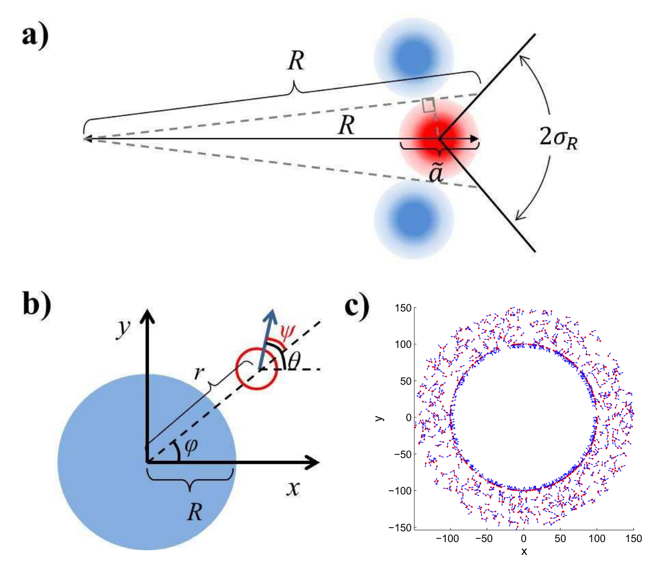
I will now test Eq. (18) by simulating a coarse-grained model of MIPS. Let us first consider what happens to an active particle in the condensed phase at the periphery that is curved (Fig. 3(a)). For such a particle, I assume that it occupies a zone of radius (shown in red) sandwiched by two zones occupied by two neighbouring particles (light blue). Note that since the concentration at the interface may not reach the level of optimal packing concentration (), should be greater than the particle’s diameter . Indeed, Fig. 2(a) suggests that the concentration is around 0.72 at the interface, which indicates that . To incorporate the effects of the neighbouring particles on the pink particle, I assume that as a result of the caging effect, the particle can only move out of the droplet if its orientation is within the range depicted. Based on the diagram shown in Fig. 3, a simple trigonometric exercise leads to
| (19) |
As expected, a lower curvature leads to a smaller escape range (smaller ).
To analyse how the variation in the escape orientation range affects the phase separated system at the steady-state, I consider a system with one condensed drop of radius co-existing with the vapour phase (Fig. 3(b)). Let me denote the particle distribution function in the vapour phase by where the first two arguments correspond to the particles’ locations and the last argument to the particles’ orientations. Due to rotational symmetry, one can eliminate one angular argument by introducing the variable [33], and study instead the reduced distribution function . On the drop’s periphery, the corresponding reduced distribution function is denoted by . Since the periphery is assumed to be infinitely thin, is only a function of and hence dimensionless. In addition, I assume that drops of all sizes have the same interior concentration , is thus related to the as follows: .
To study the distribution functions, I assume again that the vapour concentration is low enough that pairwise repulsive interactions can be ignored, and simulate the dynamics of active point particles, i.e., non-interacting active particles, in an annular geometry of inner radius and outer radius (Fig. 3(b)). As in the linear case, the particles’ orientations are randomised if they reach the outer circular boundary, while if the -th particle reaches the inner boundary, its positions will remain fixed until its orientation is within the escape range, i.e., until is between and . Simulation results are shown in (Fig. 4). Away from the interface, it is observed that the concentration rapidly reaches a stationary value for, say, (Fig. 4(a)). As expected from previous discussion, the vapor concentration goes down with since a flatter interface leads to a narrower escape range, which leads to a smaller outflux of particles from the condensed phase. Fig. 4(b) shows that decays to (the vapour concentration as ) like , which, as we have seen, is consistent the Gibbs-Thomson relation in equilibrium systems.

IV Fluctuating interface
I have so far ignored fluctuations in the interfacial profile. In reality, the interface of course fluctuates, which is already discernible from the spatially constrained system shown in Fig. 1(b). In particular, previous simulation result points to the scaling law [18]:
| (20) |
where is the steady state interfacial width:
| (21) |
with being the average position of the interface. Here, the symbol denotes the location of the interface, i.e., the location of the peak of (Fig. 2). To understand the scaling observed, let us consider the effects of interface curvature on the particle exchange dynamics. Although the previous section focuses only on a circular interface, i.e., the curvature is positive, one can easily extends Eq. (19) to allow for concave interface as well (Fig. 5). The physical motivation behind the formula is the same, a particle at a highly convex portion of the interface will have a wider escape orientation range (red particle in Fig. 5) than a particle at a highly concave interface (green particle).

Since the fluctuations ultimately come from the fluctuating dynamics of particle exchange at the interface, we need to model the steady-state dynamics of stochastically. The simplest equation of motion (EOM) for the interface that incorporates both the effects of stochasticity and curvature-modified outflux is
| (22) |
where denotes the rate of particles coming into the interface, and thus contributing to the growth of , while denotes the rate of particle escaping with the effect of local interface curvature () taken into account. The noise terms are which are Markovian, spatially independent and are either 0 or 1 with equal probability. Since the interface does not move at the steady state by assumption, has to be identical to . From now on, I will focus exclusively on the hydrodynamic limits (large temporal and spatial scales). So let us coarse grain by defining a new coarse-grained height function :
| (23) |
where and is large enough that become Gaussian as a result of the central limit theorem. The EOM of is then
| (24) | |||||
| (25) |
where are now Gaussian noises such that
| (26) | |||||
| (27) |
In the long-wavelength limit, the fluctuating term and so the only relevant fluctuations come from the Guassian fluctuations . Therefore, in the hydrodynamic limits, Eq. (25) is exactly the Edwards-Wilkinson model [34], with the effective surface tension given by . Note that the effective surface tension here is always positive, which is a requirement for having a stable interface. As such this effective surface tension is distinct from the mechanical definition of the surface tension, which has been shown to be negative in MIPS [18]. As mentioned in Section 2.2, the negative tension around the interface is likely to be caused by the particles escaping from the condensed phase that are now travelling close to being parallel to the interface. Consistent with our definition of the location of the interface (Fig. 2), these escaped particles are not considered part of the condensed phase and are thus ignored in our discussion of the interfacial fluctuations. In other words, the effective surface tension derived here is distinct from the mechanical definition of the surface tension discussed by Bialke et al [18].
Given that our stochastic model is equivalent to the Edwards-Wilkinson model, the temporal and steady-state dynamics of interfacial width is known to following the scaling form:
| (28) |
for some scaling function (Fig. 6). In a 2D system where the interface is a line, and [34, 35]. As shown in Fig. 6, these expectations are confirmed with direct simulation of a discretised version of the original EOM in Eq. (22). This model thus provides an analytical argument supporting the steady state scaling recently observed numerically [18].
To summarise this section, I have incorporated the caging effect as discussed in Sect. III into the modelling of the stochastic dynamics of particle exchanges at the interface. The model equation is then shown to be equivalent to the Edward-Wilkinson model in the hydrodynamic limits. In particular, the emergence of the effective surface tension term () from the particle dynamics at the interface also explains why the interface is flat when both phases span the system, and circular when one phase does not span the system.
V MIPS in 3D
I have so far analysed the interfacial properties in MIPS in 2D using a combination of analytical and numerical methods. Here I will extrapolate the results obtained to MIPS in 3D.
V.1 Flat interface
Employing the sharp interface model for MIPS in 3D, the pressure balance equation in Eq. (8) becomes
| (29) |
where on the R.H.S. the active force contribution corresponds to the swim pressure of active particles in 3D in the vapour phase [23], and on the L.H.S., the first terms comes from active contribution to the force assuming again that the orientation is isotropic in the condensed phase. With regards to the minimal active force required for MIPS, using the approximations that is negligible and that , we arrive at
| (30) |
which is very similar to the expression in 2D (Eq. (9)).
V.2 Spherical interface
The dimensional analysis presented in Sect. III.1 applies also spherical drops in 3D. Therefore, if the assumption that the escape range decreases with the curvature of the drop, then the Gibbs-Thomson relation should emerge in the large drop limit (Eq. (18)). In particular, we again expect the MIPS coarsening kinetics to be equivalent to the equilibrium scheme at low supersaturation [32, 36, 15].
V.3 Interface fluctuations
For MIPS in 3D, the interface is two dimensional and so there are two principal curvatures. If we adopt the natural assumption that the escape range now depends on the mean curvature, then the theoretical analysis presented in Sect. IV applies in 3D straightforwardly. As a result, keeping only the linear terms will again lead to the Edwards-Wilkinson model in the hydrodynamic limits.
VI Discussion & Outlook
In this paper I have investigated the microscopic dynamics of active particles in the interfacial regions in MIPS using a combination of simulations and analytical arguments, and demonstrated i) how interface stability is achieved, ii) why the GT relation emerges in MIPS, and iii) how interface fluctuations scale with the system size. Therefore, I have shown that all the observed “surface tension” related phenomena found in MIPS result from the microscopic dynamics of the active particles. More specifically, I have demonstrated that pressure balance in MIPS is achieved because of the orientation anisotropy in the region, which leads to a high active force directed towards the condensed phase. By incorporating the caging effects of neighbouring particles in the peripheral of a condensed drop, I have shown how the Gibbs-Thomson relation emerges naturally in MIPS, which dictates that the larger the condensed drop, the smaller the vapour concentration outside the drop. If the supersaturation level is small, the GT relation leads to diffusive transfer of active particles from small drops to larger drops. As a result, the late-stage coarsening kinetics in an active phase-separating system should follow the temporal scaling as in equilibrium phase separation: i.e., the average droplet size in the system goes like [32, 36, 15]. In addition, the droplet size distribution should approach asymptotically the universal size distribution obtained by Lifshitz and Slyozov [32]. Lastly, motivated by the same caging effects, I have proposed a stochastic model that describes the interfacial fluctuations in MIPS. In this model, the probability of particles leaving the interface is assumed to be dependent on the interface curvature. Analytical argument is then provided to show that the proposed model belongs to the same universality class of the Edwards-Wilkinson model.
There are a number of future directions that are of interest. For instance, phase separation may play a role in the cytoplasmic re-organisation during asymmetric cell division [37, 38]. How the activity in the cytoplasm due to the many motor proteins contribute to such re-organisation via phase separation awaits more attention. Moreover, the fact that active phase separation occurs naturally begs the question of the existence of the critical point as in the equilibrium case. The critical transition in incompressible active fluids has recently been shown to give rise to a novel universality class [39]. And if a critical transition exists in MIPS, will the critical exponents be identical to those in the equilibrium case which belong to the 2D Ising Universality class? This question awaits further investigation.
Appendix
Appendix A Simulation details
A.1 Particle dynamics simulation
For the simulation results reported in Sect. II (Figs 1 & 2), I numerically integrating the Langevin equations for each particle in the bulk of the system of size by using the following updates:
| (31) | |||||
| (32) |
where are Gaussian distributed random variables with zero mean and unit variance, is given by the Weeks-Chandler-Andersen potential shown in Eq. (3). Periodic boundary condition is enforced in the , direction; while in the direction, if , then it is reset to zero, and if , then and is an angle chosen at random.
The parameters of the simulations are: , , , , , for repulsive particles and for point particles. The system has width and height , with 300 particles initialized in the configuration of a hexagonal lattice (with spacing 1) next to the left boundary, and random orientations. Two hundred million time steps are evolved to equilibrate the system and then data are collected in the subsequent two hundred million time steps.
A.2 Point particles in an annular geometry
For the simulation results reported in Sect. III (Figs 3), the system is now annular with inner radius and outer radius . The same updates as in Eqs (31) and (32) are performed for the point particles in the bulk of the system. Concerning the boundary conditions, if then the particle becomes part of the condensed drop periphery, and the orientation follows the update:
| (33) |
while the position remains the same until (Fig. 3(b)), in which case the particle leaves the condensed phase. If , then and is an angle chosen at random.
For distinct annulus geometry, the density is normalised by , which is the density of particles at the inner circular wall. This is based on the assumption that is the same irrespective of drop sizes.
The parameters of the simulations are: , , , , . The system has 1000 particles initialized with random orientations and positions. Twenty million time steps are evolved to equilibrate the system and then data are collected in the subsequent twenty million time steps. Simulations are performed for and while is always .
A.3 Fluctuating interfaces
To simulate interface fluctuations according to Eq. (22), I discretise the interface (a line) into sites with height values where . Periodic boundary condition is enforced. The updates are performed as follows:
| (34) | |||||
where are either 0 or 1 chosen with equal probability, and . The system sizes simulated are and . The total number of time steps simulated for each system size is .
I thank Christoph Weber (Max Planck Institute for the Physics of Complex Systems), Fernando Peruani (Université Nice Sophia Antipolis) and Richard Sear (University of Surrey) for stimulating discussions and for their comments on the manuscript.
References
- [1] C. Domb, J. L. Lebowitz, and M. S. Green, Phase Transitions and Critical Phenomena, v. 8 (Academic Press, 1983), ISBN 9780122203084, URL http://books.google.co.uk/books?id=najcQgAACAAJ.
- [2] A. J. Bray, Advances in Physics 51, 481 (2002), URL http://dx.doi.org/10.1080/00018730110117433.
- [3] J. Tailleur and M. E. Cates, Physical review letters 100, 218103 (2008), ISSN 0031-9007, URL http://journals.aps.org/prl/abstract/10.1103/PhysRevLett.100.218103.
- [4] M. E. Cates, D. Marenduzzo, I. Pagonabarraga, and J. Tailleur, Proceedings of the National Academy of Sciences 107, 11715 (2010), URL http://www.pnas.org/content/107/26/11715.abstract.
- [5] F. Peruani, T. Klauss, A. Deutsch, and A. Voss-Boehme, Physical Review Letters 106, 128101 (2011), URL http://link.aps.org/doi/10.1103/PhysRevLett.106.128101.
- [6] J. P. D. Clewett, K. Roeller, R. M. Bowley, S. Herminghaus, and M. R. Swift, Physical Review Letters 109, 228002 (2012), URL http://link.aps.org/doi/10.1103/PhysRevLett.109.228002.
- [7] F. D. C. Farrell, M. C. Marchetti, D. Marenduzzo, and J. Tailleur, Physical Review Letters 108, 248101 (2012), URL http://dx.doi.org/10.1103/PhysRevLett.108.248101.
- [8] Y. Fily and M. C. Marchetti, Physical Review Letters 108, 235702 (2012), URL http://link.aps.org/doi/10.1103/PhysRevLett.108.235702.
- [9] J. Schwarz-Linek, C. Valeriani, A. Cacciuto, M. E. Cates, D. Marenduzzo, A. N. Morozov, and W. C. K. Poon, Proceedings of the National Academy of Sciences 109, 4052 (2012), URL http://www.pnas.org/content/109/11/4052.abstract.
- [10] M. E. Cates and J. Tailleur, EPL (Europhysics Letters) 101, 20010 (2013), URL http://stacks.iop.org/0295-5075/101/i=2/a=20010.
- [11] G. S. Redner, M. F. Hagan, and A. Baskaran, Physical Review Letters 110, 55701 (2013), URL http://link.aps.org/doi/10.1103/PhysRevLett.110.055701.
- [12] J. Bialké, H. Löwen, and T. Speck, EPL (Europhysics Letters) 103, 30008 (2013), URL http://stacks.iop.org/0295-5075/103/i=3/a=30008.
- [13] I. Buttinoni, J. Bialké, F. Kümmel, H. Löwen, C. Bechinger, and T. Speck, Physical Review Letters 110, 238301 (2013), URL http://link.aps.org/doi/10.1103/PhysRevLett.110.238301.
- [14] J. Stenhammar, A. Tiribocchi, R. J. Allen, D. Marenduzzo, and M. E. Cates, Physical Review Letters 111, 145702 (2013), URL http://link.aps.org/doi/10.1103/PhysRevLett.111.145702.
- [15] R. Wittkowski, A. Tiribocchi, J. Stenhammar, R. J. Allen, D. Marenduzzo, and M. E. Cates, Nature Communications 5, 4351 (2014), URL http://dx.doi.org/10.1038/ncomms5351.
- [16] A. Y. Grosberg and J. F. Joanny, Physical Review E 92, 32118 (2015), URL http://link.aps.org/doi/10.1103/PhysRevE.92.032118.
- [17] J. Stenhammar, R. Wittkowski, D. Marenduzzo, and M. E. Cates, Physical Review Letters 114, 18301 (2015), URL http://link.aps.org/doi/10.1103/PhysRevLett.114.018301.
- [18] J. Bialké, J. T. Siebert, H. Löwen, and T. Speck, Physical Review Letters 115, 98301 (2015), URL http://link.aps.org/doi/10.1103/PhysRevLett.115.098301.
- [19] R. P. Sear, arXiv:1503.06963 p. 0 (2015), URL http://arxiv.org/abs/1503.06963.
- [20] A. Marchand, J. H. Weijs, J. H. Snoeijer, and B. Andreotti, American Journal of Physics 79, 999 (2011), URL http://scitation.aip.org/content/aapt/journal/ajp/79/10/10.1119/1.3619866.
- [21] J. D. Weeks, D. Chandler, and H. C. Andersen, The Journal of Chemical Physics 54, 5237 (1971), URL http://scitation.aip.org/content/aip/journal/jcp/54/12/10.1063/1.1674820.
- [22] C. F. Lee, New Journal of Physics 15, 055007 (2013).
- [23] S. C. Takatori, W. Yan, and J. F. Brady, Physical Review Letters 113, 28103 (2014), URL http://link.aps.org/doi/10.1103/PhysRevLett.113.028103.
- [24] X. Yang, M. L. Manning, and M. C. Marchetti, Soft Matter 10, 6477 (2014), URL http://dx.doi.org/10.1039/C4SM00927D.
- [25] S. A. Mallory, A. Šarić, C. Valeriani, and A. Cacciuto, Physical Review E 89, 52303 (2014), URL http://link.aps.org/doi/10.1103/PhysRevE.89.052303.
- [26] A. P. Solon, Y. Fily, A. Baskaran, M. E. Cates, Y. Kafri, M. Kardar, and J. Tailleur, Nature Physics 11, 673 (2015a), URL http://dx.doi.org/10.1038/nphys3377.
- [27] J.-P. Hansen and I. R. McDonald, Theory of Simple Liquids (Academic Press, 2006), ISBN 0123705355, URL http://www.amazon.ca/exec/obidos/redirect?tag=citeulike09-20{&}path=ASIN/0123705355.
- [28] P. G. de Gennes and J. Prost, The Physics of Liquid Crystals (International Series of Monographs on Physics) (Oxford University Press, USA, 1995), ISBN 0198517858, URL http://www.amazon.ca/exec/obidos/redirect?tag=citeulike09-20{&}path=ASIN/0198517858.
- [29] A. P. Solon, J. Stenhammar, R. Wittkowski, M. Kardar, Y. Kafri, M. E. Cates, and J. Tailleur, Physical Review Letters 114, 198301 (2015b), URL http://link.aps.org/doi/10.1103/PhysRevLett.114.198301.
- [30] J. Stenhammar, D. Marenduzzo, R. J. Allen, and M. E. Cates, Soft Matter 10, 1489 (2014), ISSN 1744-683X, URL http://xlink.rsc.org/?DOI=C3SM52813H.
- [31] R. G. Winkler, A. Wysocki, and G. Gompper, Soft Matter 11, 6680 (2015), ISSN 1744-683X, URL http://xlink.rsc.org/?DOI=C5SM01412C.
- [32] I. Lifshitz and V. Slyozov, Journal of Physics and Chemistry of Solids 19, 35 (1961), URL http://dx.doi.org/10.1016/0022-3697(61)90054-3.
- [33] A. Pototsky and H. Stark, EPL (Europhysics Letters) 98, 50004 (2012), URL http://stacks.iop.org/0295-5075/98/i=5/a=50004.
- [34] S. F. Edwards and D. R. Wilkinson, Proceedings of the Royal Society of London A: Mathematical, Physical and Engineering Sciences 381, 17 (1982), URL http://rspa.royalsocietypublishing.org/content/381/1780/17.abstract.
- [35] A. L. Barabási and H. E. Stanley, Fractal Concepts in Surface Growth (Cambridge University Press, 1995), ISBN 0521483182, URL http://www.amazon.ca/exec/obidos/redirect?tag=citeulike09-20{&}path=ASIN/0521483182.
- [36] J. Yao, K. R. Elder, H. Guo, and M. Grant, Physical Review B 45, 8173 (1992), URL http://dx.doi.org/10.1103/PhysRevB.45.8173.
- [37] C. Brangwynne, C. Eckmann, D. Courson, A. Rybarska, C. Hoege, J. Gharakhani, F. Jülicher, and A. Hyman, Science 324, 1729 (2009), URL http://dx.doi.org/10.1126/science.1172046.
- [38] C. F. Lee, C. P. Brangwynne, J. Gharakhani, A. A. Hyman, and F. Julicher, Physical Review Letters 111, 088101 (2013).
- [39] L. Chen, J. Toner, and C. F. Lee, New Journal of Physics 17, 042002 (2015).