Change point analysis of second order characteristics in non-stationary time series

Holger Dette Affiliation: Ruhr-Universität Bochum Affiliation: Fakultät für Mathematik Affiliation: 44780 Bochum Affiliation: Germany Affiliation: email: holger.dette@ruhr-uni-bochum.de Weichi Wu Affiliation: University of Toronto Affiliation: 100 St. George St. Affiliation: Toronto ON M5S 3G3 Affiliation: Canada Affiliation: email: weichi.wu@utoronto.ca Zhou Zhou Affiliation: University of Toronto Affiliation: 100 St. George St. Affiliation: Toronto ON M5S 3G3 Affiliation: Canada Affiliation: email: zhou@utstat.toronto.edu

Abstract

A restrictive assumption in the work on testing for structural breaks in time series consists in the fact that the model is formulated such that the stochastic process under the null hypothesis of “no change-point” is stationary. This assumption is crucial to derive (asymptotic) critical values for the corresponding testing procedures using an elegant and powerful mathematical theory, but it might be not very realistic from a practical point of view. For example, if change point analysis for a particular parameter of the process (such as the variance) is performed, it is not necessary clear why other parameters (such as the mean or higher order moments) have to stay constant under the hypothesis that there is no change point in the parameter of interest.
This paper develops change point analysis under less restrictive assumptions and deals with the problem of detecting change points in the marginal variance and correlation structures of a non-stationary time series. A CUSUM approach is proposed, which is used to test the “classical” hypothesis of the form $H_{0}:\theta_{1}=\theta_{2}$ vs. $H_{1}:\theta_{1}\not=\theta_{2}$ , where $\theta_{1}$ and $\theta_{2}$ denote second order parameters (such as the variance or the lag $k$ -correlation) of the process before and after a change point. The asymptotic distribution of the CUSUM test statistic is derived under the null hypothesis. This distribution depends in a complicated way on the dependency structure of the nonlinear non-stationary time series and a bootstrap approach is developed to generate critical values. The results are then extended to test the hypothesis of a non relevant change point, i.e. $H_{0}:|\theta_{1}-\theta_{2}|\leq\delta$ , which reflects the fact that inference should not be changed, if the difference between the parameters before and after the change-point is small.
In contrast to previous work, our approach does neither require the mean to be constant nor - in the case of testing for lag $k$ -correlation - that the mean, variance and fourth order joint cumulants are constant under the null hypothesis. In particular, we allow that the variance has a change point at a different location than the auto-covariance. The results are illustrated by means of a simulation study, which shows that the new procedures have nice finite sample properties. The central England monthly temperature series are analyzed and significant change points in the variance and lag $1$ -correlation are found in the winter monthly temperature at the late 19th century.

AMS subject classification: 62M10, 62F05, 62G09

Keywords and phrases: piecewise locally stationary process, change point analysis, relevant change points, second order structure, local linear estimation

1 Introduction

Change point analysis is a well studied subject in the statistical literature. Since the seminal work on detecting structural breaks in the mean of Page, (1954) a powerful methodology has been developed to detect various types of change points in time series [see for example Aue and Horváth, (2013) and Jandhyala et al., (2013) for recent reviews of the literature]. Several authors have argued that in applications besides the mean the detection of changes in the variance or the correlation structure of a time series is of importance as well. Typical examples include the discrimination between stages of high and low asset volatility or the detection of changes in the parameters of an AR( $p$ ) model in order to obtain superior forecasting procedures. Wichern et al., (1976) studied the change point problem for the variance in a first order autoregressive model. These authors pointed out that - even if log-return data exhibits a stationary behavior in the mean - the variability is often not constant and as a consequence any conclusions based on the assumption of homoscedasticity could be misleading. Abraham and Wei, (1984) and Baufays and Rasson, (1985) used a Bayesian and an ML approach to find change points in AR-models. Inclán and Tiao, (1994) proposed a nonparametric CUSUM-type test for changes in the variance of an independent identically distributed sequence and Lee and Park, (2001) derived corresponding results applicable to linear processes [see also Chen and Gupta, (1997) who used the Schwarz information criterion]. Recently Galeano and Peña, (2007) and Aue et al., (2009) suggested nonparametric tests for structural breaks in the variance matrix of a multivariate time series, while Davis et al., (2006) and Preuss et al., (2014) proposed methods for detecting multiple breaks in piecewise stationary processes.
This list of references is by no means complete but an important feature of the cited references and most of the literature on testing for structural breaks consists in the fact that the model is formulated such that the stochastic process under the null hypothesis of “no change-point” is stationary. This assumption is crucial to derive (asymptotic) critical values for the corresponding testing procedures using an elegant and powerful mathematical theory such as strong approximations or invariance principles. On the other hand this assumption drastically restricts the applicability of the methodology. For example, Inclán and Tiao, (1994) and Aue et al., (2009) assume for the construction of a testing procedure for the hypothesis

\displaystyle H_{0}:\ \sigma^{2}_{i}=\sigma^{2}_{j}~\ \text{ for all}\ i,j=1,\ldots,n~\text{ versus }\ H_{1}:\ \sigma^{2}_{i}\neq\sigma^{2}_{j}\ \text{for some}\ i\neq j.

(1.1)

of a constant variance of a time series that the mean of the sequence under consideration does not change in time (as the variance under the null hypothesis). A similar assumption was made by Wied et al., (2012) in the context of testing for a constant correlation, where the authors suggested a CUSUM-type statistic for a change in the correlation of a stationary time series if at the same the means and variances do not change. However, from a practical point of view, assumptions of this type are very restrictive and there might be many situations where one is interested in a change of the variance (or the correlation) even if the mean (or the means and the variances) change gradually in time. In this case the classical approach is not applicable any more. Recently, Zhou, (2013) investigated such a problem, in the context of testing for a constant mean, and demonstrated that the classical CUSUM approach yields to severe biased testing results if the assumption of (weak) stationarity (under the null hypothesis) is not satisfied.

The situation gets even more complicated if one is interested in more sophisticated hypotheses such as precise hypotheses [see Berger and Delampady, (1987)]. Here (in the simplest case) one assumes the existence of a change point $k\in\{1,\ldots,n\}$ such that

\displaystyle v_{1}=\sigma_{1}^{2}=\ldots=\sigma_{k}^{2}~\not=~v_{2}=\sigma_{k+1}^{2}=\ldots=\sigma_{n}^{2}~,

(1.2)

and is interested in hypotheses of the form

\displaystyle H_{0}:\Delta:=|v_{2}-v_{1}|\leq\delta\ \ \text{versus}\ \ H_{1}:\Delta:=|v_{2}-v_{1}|>\delta

(1.3)

for some pre-specified constant $\delta>0$ . Throughout this paper we call hypotheses of the form (1.1) “classical” in order to distinguish these from the precise hypotheses of the form (1.3). Although hypotheses of the form (1.3) have been discussed in other fields [see Chow and Liu, (1992) and Mcbride, (1999)] the problem of testing precise hypotheses has only recently been considered by Dette and Wied, (2014) in the context of change point analysis. These authors point out that in many cases a modification of the statistical analysis might not be necessary if a change point has been identified but the difference between the parameters before and after the change-point is rather small. In particular, inference might be robust under “small” changes of the parameters and changing decisions (such as trading strategies or modifying a manufacturing process) might be very expensive and should therefore only be performed if changes would have serious consequences. Testing hypothesis of the form (1.3) to detect a structural break also avoids the consistency problem mentioned in Berkson, (1938), that is: any test will detect negligible changes in the parameter if the sample size is sufficiently large. Dette and Wied, (2014) call the hypotheses of the form (1.3) hypotheses of a non relevant (null hypothesis) and relevant change point (alternative), and according to their argumentation only relevant change points should be detected, because one has to distinguish scientific from statistical significance.
Although the formulation of the testing problem in the form (1.3) is appealing, the construction of corresponding tests faces several mathematical challenges. In particular, one has to deal with the problem of non-stationarity (even under the null hypothesis of a non relevant change point). For example, Dette and Wied, (2014) developed a CUSUM-type test for the hypotheses in (1.3), which is only applicable under the assumption that the time series before and after the change point is strictly stationary. From a practical point this assumption seems to be very strong and not very realistic.

The present paper is devoted to the construction of change point tests for the second-order characteristics of a non-stationary time series, in particular changes in the variance and the lag $k$ -correlation. We consider piecewise locally stationary processes as discussed by Zhou, (2013), which are introduced in Section 2. Section 3 is devoted to the “classical” change point problem for the variance or lag $k$ -correlation of a piecewise locally stationary process. We propose a CUSUM approach based on nonparametric residuals and prove weak convergence of the corresponding CUSUM statistic. It turns out that the limiting distribution depends in a complicated way on the dependence structure of the piecewise locally stationary process, and for this reason a wild bootstrap approach is developed and its consistency proved. The methodology is very general and applicable in many situations where the assumptions of classical tests are not satisfied. For example, in the problem of testing the “classical” hypothesis of a change in the lag $k$ -correlation we do neither assume that the mean, variance or higher order joint cumulants of the nonstationary sequence are constant nor that the change in the variance and the lag $k$ -correlation occur at the same location. Furthermore, we discover in this paper that the stochastic errors produced in the nonparametric estimation of the mean and variance function are asymptotically negligible in the second-order CUSUM statistic. The result is of particular interest and highly non-trivial because the order of the latter nonparametric errors are larger than the $1/\sqrt{n}$ convergence rate of the CUSUM test.

Section 4 is devoted to the problem of testing the hypothesis of a non relevant change in the variance or lag $k$ -correlation. We use the CUSUM approach proposed in Dette and Wied, (2014) to obtain a test for the hypothesis (1.3) and its analogue in the case of lag $k$ -correlations. Asymptotic normality of a corresponding $\mathcal{L}_{2}$ -type statistic is established and a wild bootstrap method is developed, which addresses the particular structure of the hypotheses in relevant change point analysis. To our best knowledge resampling procedures for this type of change point analysis in non-stationary nonparametric problems have not been considered in the literature so far. The finite sample properties of the new procedures are investigated by means of a simulation study in Section 5. In Section 6, we analyze the central England monthly temperature series and illustrate the usefulness of the proposed methodology in identifying second order change points in climate data. Finally, all proofs and technical details are deferred to an appendix and an online supplement, respectively.

2 Piecewise locally stationary processes

We start introducing some notations, which we frequently use throughout this paper. For a (real valued) random variable $X$ and $p\geq 1$ we denote by $\|X\|_{p}=(\mathbb{E}|X|^{p})^{1/p}$ the $\mathcal{L}_{p}$ norm of $X$ . The symbol $\stackrel{{\scriptstyle\cal D}}{{\longrightarrow}}$ means weak convergence of real valued random variables (convergence in distribution). For any interval $\mathcal{I}\subset\mathbb{R}$ and nonnegative integer $q$ define $\mathcal{C}^{q}(\mathcal{I})$ as the set of $q$ times continuously differentiable functions $f:\mathcal{I}\to\mathbb{R}$ and $\mathcal{C}(\mathcal{I})=\mathcal{C}^{0}(\mathcal{I})$ . Let $\{\varepsilon_{i}\}_{i\in\mathbb{Z}}$ denote a sequence of independent identically distributed (i.i.d.) random variables and denote by $\mathcal{F}_{i}=\sigma(...,\varepsilon_{0},...,\varepsilon_{i-1},\varepsilon_{i})$ the sigma field generated by $\{\varepsilon_{j}|j\leq i\}$ . We define the sigma field $\mathcal{F}_{i}^{(j)}=\sigma(...,\varepsilon_{j-1},\varepsilon^{\prime}_{j},\varepsilon_{j+1}...,\varepsilon_{i})$ , where $\{\varepsilon^{\prime}_{i}\}_{i\in\mathbb{Z}}$ is an independent copy of $\{\varepsilon_{i}\}_{i\in\mathbb{Z}}$ , and $\mathcal{F}_{i}^{*}=\mathcal{F}_{i}^{(0)}$ for short. In the following discussion we will also make frequent use of the projection operator $\mathcal{P}_{j}(\cdot)=\mathbb{E}(\cdot|\mathcal{F}_{j})-\mathbb{E}(\cdot|\mathcal{F}_{j-1})$ .

In this paper, we consider the model

\displaystyle Y_{i}=\mu(t_{i})+e_{i},\qquad i=1,\dots,n,

(2.1)

where (for the sake of simplicity) $t_{i}=i/n$ ( $i=1,\ldots,n$ ) and $\mu$ is a smooth function. Note that formally $\{Y_{i}\}_{i=1}^{n}$ is a triangular array of random variables but we do not reflect this fact in our notation. Change point problems for this model have found considerable attention in the recent literature, where most of the work refers to problems of detecting a gradual change of the mean in the situation of zero mean and independent identically distributed (i.i.d.) errors (even assumed to be Gaussian in some cases) [see Müller, (1992) for an early reference and Mallik et al., (2011) and Mallik et al., (2013) for more recent references]. Recently Vogt and Dette, (2015) proposed a generalized CUSUM approach to detect gradual changes in model (2.1) using a different concept of local stationarity [see Vogt, (2012)].
In the present paper we consider non-stationary processes of the form (2.1) and are interested in identifying abrupt changes in the second order properties such as the variance or the correlation at a given lag. More precisely we consider an error process $\{e_{i}\}_{i=1}^{n}$ in (2.1), which is piecewise locally stationary (PLS) with $r$ breaks for some $r\in\mathbb{N}$ . Formally, we use the following definition for a $PLS$ process and the concept of “physical dependence measure for PLS”, which is given in Zhou, (2013).

Definition 2.1.

(1) The sequence $\{e_{i}\}_{i=1}^{n}$ is called PLS with $r$ break points if there exist constants $0=b_{0}<b_{1}<...<b_{r}<b_{r+1}=1$ and nonlinear filters $G_{0},G_{1},...,G_{r}$ , such that

\displaystyle e_{i}=G_{j}(t_{i},\mathcal{F}_{i}),\mbox{ if }b_{j}<t_{i}\leq b_{j+1},

where $\mathcal{F}_{i}=\sigma(...,\varepsilon_{0},...,\varepsilon_{i-1},\varepsilon_{i})$ , and $\{\varepsilon_{i}\}_{i\in\mathbb{Z}}$ is a sequence of i.i.d. random variables.

(2) Assume that $\max_{1\leq i\leq n}\|e_{i}\|_{p}<\infty$ for some $p\geq 1$ . Then for $k>0$ , define the $k$ th physical dependence measure in $\mathcal{L}_{p}$ -norm as

\displaystyle\delta_{p}(k)=\max_{0\leq i\leq r}\sup_{b_{i}<t\leq b_{i+1}}\|G_{i}(t,\mathcal{F}_{k})-G_{i}(t,\mathcal{F}_{k}^{*})\|_{p},

where $\delta_{p}(k)=0$ if $k<0$ .

For the asymptotic analysis presented later in this paper we list the following conditions:

(A1) The process $\{e_{i}\}^{n}_{i=1}$ is PLS and piecewise stochastic Lipschitz continuous. This means that there exists a constant $C>0$ , such that for all $i\in\{0,\dots,r\}$ and all $t,s\in[b_{i},b_{i+1}]$ the condition

\displaystyle\|G_{i}(t,\mathcal{F}_{0})-G_{i}(s,\mathcal{F}_{0})\|_{\iota}/(t-s)\leq C(t-s)

holds, where $\iota\geq 8$ and $C$ denotes a positive constant. In addition, $\mathbb{E}[e_{i}]=0$ for all $1\leq i\leq n$ , and we assume the existence of a strictly positive variance function $\sigma^{2}:[0,1]\to\mathbb{R}^{+}$ , such that $\sigma^{2}_{i}:=\sigma^{2}(t_{i})={\rm Var}(e_{i})\ (i=1,\dots,n).$

(A2) The second derivative $\ddot{\mu}$ of the function $\mu$ in model (2.1) exists and is Lipschitz continuous on the interval $[0,1]$ .

(A3) $\max_{0\leq i\leq r}\sup_{t\in(b_{i},b_{i+1}]}\|G_{i}(t,\mathcal{F}_{0})\|_{\iota}<\infty$ for some $\iota\geq 8$ .

(A4) $\delta_{\iota}(k)=O(\chi^{k})$ for some $\chi\in(0,1)$ and some $\iota\geq 8$ .

Remark 2.1.

a) We emphasize that the bound of $\max_{1\leq i\leq n}\|e_{i}\|_{p}$ in Definition 2.1 does not depend on $n$ . This assumption is made in order to simplify the assumptions and the proofs in the subsequent discussion. It is also possible to develop corresponding results for an $n$ -dependent bound with an additional complication in the technical arguments of the proofs and in the assumptions.
b) Note that the process $\{e_{i}^{2}\}^{n}_{i=1}$ of squared errors is also PLS. Simple calculations show that $\{e_{i}^{2}\}^{n}_{i=n}$ satisfies the assumptions (A1), (A3), (A4) with $\iota\geq 4$ .

3 Tests for changes in the second order structure

Suppose that we observe data $\{Y_{i}\}_{i=1}^{n}$ according to model (2.1), where the process $\{e_{i}\}_{i=1}^{n}$ is PLS and $\mu$ is an unknown deterministic trend. We are interested in testing nonparametrically the “classical” hypothesis of a change point in the variance or the lag $k$ -correlation. The important difference to previous work on this subject [see for example Inclán and Tiao, (1994) or Aue et al., (2009)] is that in general the process is NOT assumed to be stationary under the null hypothesis of no change point. This means - for example - that the approach proposed here can be used to test the hypotheses (1.1), where the mean is not constant. The price for this type of flexibility is that critical values of the asymptotic distribution of the CUSUM statistic are not directly available. For the solution of this problem we will develop a bootstrap CUSUM-type test for the “classical” hypotheses of a change point in the variance or lag $k$ -correlation, which is based on residuals from a local linear fit. For the definition of the local linear estimator we assume throughout this paper that the corresponding kernel function, say $K$ , is symmetric with support $[-1,1]$ satisfying $\int K(x)dx=1$ , and define for $b>0$ the function $K_{b}(\cdot)=K(\frac{\cdot}{b})$ . The moments of $K$ and $K^{2}$ are denoted by $\mu_{l}=\int_{\mathbb{R}}x^{l}K(x)dx$ and $\phi_{l}=\int_{\mathbb{R}}x^{l}K^{2}(x)dx$ , respectively ( $l=0,1,\ldots$ ). We also assume that $K\in\mathcal{C}^{(2)}([-1,1])$ .

3.1 Change point tests for the variance

Our first goal is to investigate the stability of the variances $\sigma^{2}_{i}=\sigma^{2}(t_{i})=\mbox{Var}(Y_{i})\ (i=1,\dots,n)$ testing nonparametrically the “classical” hypotheses (1.1). For this purpose we consider the CUSUM statistic

\displaystyle\hat{T}_{n}=\max_{1\leq i\leq n}\Big|\hat{S}_{i}-\frac{i}{n}\hat{S}_{n}\Big|,

(3.1)

where $\hat{S}_{i}=\sum_{j=1}^{i}\hat{e}_{j}^{2}$ denotes the sum of squared nonparametric residuals $\hat{e}_{i}=Y_{i}-\hat{\mu}_{b_{n}}(t_{i})$ , and $\hat{\mu}_{b_{n}}({\cdot})$ is the local linear estimator of the function $\mu$ with bandwidth $b_{n}$ , that is

\displaystyle(\hat{\mu}_{b_{n}}(t),\hat{\dot{\mu}}_{b_{n}}(t))=\mathop{\mbox{argmin}}_{b_{0},b_{1}}\sum^{n}_{i=1}\big(Y_{i}-b_{0}-b_{1}(t_{i}-t)\big)^{2}K_{b_{n}}(t_{i}-t)

(3.2)

[see Fan and Gijbels, (1996)]. Weak convergence of the statistic $\hat{T}_{n}/\sqrt{n}$ follows under the additional assumption

(A5) The long run variance function

\kappa_{1}^{2}(t)=\sum_{k=-\infty}^{\infty}\text{cov}(G^{2}_{i}(t,\mathcal{F}_{k}),G^{2}_{i}(t,\mathcal{F}_{0}))\qquad\text{if $t\in(b_{i},b_{i+1}]$},

(3.3)

exists, $\kappa_{1}^{2}(0):=\lim_{t\downarrow 0}\kappa^{2}_{1}(t)$ exists and $\inf_{t\in[0,1]}\kappa_{1}^{2}(t)>0$ .

The following result provides the asymptotic distribution of $\hat{T}_{n}$ . Its proof is complicated and therefore deferred to Section 7.1.1 in the Appendix.

Theorem 3.1.

If assumptions (A1)-(A5) are satisfied and $nb^{6}_{n}\rightarrow 0$ , $nb^{3}_{n}\rightarrow\infty$ , then under the null hypothesis of no change in the variance we have

\displaystyle\frac{1}{\sqrt{n}}\hat{T}_{n}\stackrel{{\scriptstyle\cal D}}{{\longrightarrow}}\mathcal{K}_{1}:=\sup_{t\in(0,1)}|U_{1}(t)-tU_{1}(1)|,

(3.4)

where $\{U_{1}(t)\}_{t\in[0,1]}$ is a zero mean Gaussian process with covariance function

\gamma(t,s)=\int_{0}^{\min(t,s)}\kappa_{1}^{2}(r)dr.

(3.5)

It follows from the proof of Theorem 3.1 that the statistic $\frac{1}{\sqrt{n}}\hat{T}_{n}$ has the same limit distribution as the statistic which is obtained if the nonparametric residuals $\hat{e}_{i}$ are replaced by the “true” errors $e_{i}$ from model (2.1). This observation is remarkable and highly non-trivial because the error from the nonparametric estimation is larger than $1/\sqrt{n}$ .

As a consequence of Theorem 3.1, we obtain - in principle - an asymptotic level $\alpha$ test for the hypothesis (1.1) by rejecting $H_{0}$ , whenever $\frac{1}{\sqrt{n}}\hat{T}_{n}>q_{1-\alpha},$ where $q_{1-\alpha}$ is the $(1-\alpha)$ -quantile of the distribution of the random variable $\mathcal{K}_{1}$ in (3.4). However, under non-stationarity (more precisely under the PLS assumption), the function $\kappa^{2}_{1}$ defined in (3.3) and, as a consequence, the covariance structure of the Gaussian process $\{U_{1}(t)-tU_{1}(1)\}_{t\in[0,1]}$ involves the complex dependency structure of the data generating process. Therefore it is very difficult to estimate the critical value $q_{1-\alpha}$ of the asymptotic distribution of the CUSUM test statistic directly. As an alternative, a data-driven critical value will be derived in the following discussion using a wild bootstrap method to mimic the distributional properties of the Gaussian process $U_{1}(\cdot)$ . Following Zhou, (2013) we define for a fixed window size, say $m$ , the quantity

\displaystyle\hat{\Phi}_{i,m}=\frac{1}{\sqrt{m(n-m+1)}}\sum_{j=1}^{i}\Big(\hat{S}_{j,m}-\frac{m}{n}\hat{S}_{n}\Big)R_{j},\qquad i=1,...,n-m+1,

(3.6)

where $\hat{S}_{j,m}=\sum_{r=j}^{j+m-1}\hat{e}_{r}^{2}$ and $\{R_{i}\}_{i\in\mathbb{Z}}$ is a sequence of i.i.d standard normal distributed random variables, which is independent of $\{\varepsilon_{i}\}_{i\in\mathbb{Z}}$ .

Theorem 3.2.

Suppose that the conditions of Theorem 3.1 are satisfied. In addition, assume that $m\rightarrow\infty$ , $m/n\rightarrow 0$ , $mb_{n}^{4}{\log^{2}n}\rightarrow 0$ and $\frac{m\log^{2}n}{nb_{n}^{3/2}}\rightarrow 0$ . Then

\displaystyle M_{n}=\max_{m+1\leq i\leq n-m+1}\Big|{\hat{\Phi}}_{i,m}-\frac{i}{n-m+1}{\hat{\Phi}}_{n-m+1,m}\Big|\stackrel{{\scriptstyle\cal D}}{{\longrightarrow}}\mathcal{K}_{1}

conditional on $\mathcal{F}_{n}$ , where the random variable $\mathcal{K}_{1}$ is defined in (3.4).

Theorem 3.2 provides an asymptotic level $\alpha$ test for the hypothesis of a constant variance in model (2.1), where the critical values are obtained by resampling. The details are summarized in the following algorithm. Some illustrations of this method are given in Section 5 and 6.

Algorithm 3.1.

[1] Calculate the statistic $\hat{T}_{n}$ defined in (3.1).

[2] Generate $B$ conditionally $i.i.d$ copies $\{\hat{\Phi}^{(r)}_{i,m}\}_{i=1}^{n-m+1}$ $(r=1,\dots,B)$ of the random variables $\{\hat{\Phi}_{i,m}\}_{i=1}^{n-m+1}$ defined in (3.6) and calculate

M_{r}=\max_{m+1\leq i\leq n-m+1}\Big|\hat{\Phi}_{i,m}^{(r)}-\frac{i}{n-m+1}\hat{\Phi}^{(r)}_{n-m+1,m}\Big|.

[3] Let $M_{(1)}\leq M_{(2)}\leq...\leq M_{(B)}$ denote the order statistics of $M_{1},\dots,M_{B}$ . The null hypothesis of constant variance is rejected at level $\alpha$ , whenever

\hat{T}_{n}/\sqrt{n}>M_{\lfloor B(1-\alpha)\rfloor}.

(3.7)

The $p$ -value of this test is given by $1-\frac{B^{*}}{B}$ , where $B^{*}=\max\{r:M_{(r)}\leq\hat{T}_{n}/\sqrt{n}\}$ .

Remark 3.1.

it follows by similar arguments as given in the proof of Theorem 2, Proposition 3 of Zhou, (2013), and Lemma 8.1 and Lemma 8.2 in the appendix of this paper that the bootstrap test (3.7) is consistent. In fact the test is able to detect local alternatives of the form $\sigma^{2}(\cdot)=\sigma^{2}+n^{-1/2}f(\cdot)$ , where $f(\cdot)$ is a nonconstant piecewise Lipschitz continuous function.

3.2 Changes in the correlation

In this section we consider the problem of testing whether there are changes in the correlation $\rho_{i,k}:=corr(Y_{i},Y_{i+k})$ for some pre-specified lag $k$ . Namely, we are interested in testing the hypotheses

\displaystyle H_{0}:\ \rho_{i,k}=\rho_{j,k}\ \text{ for all}\ i,j=1,\ldots,n~\text{ versus}\ H_{1}:\ \rho_{i,k}\neq\rho_{j,k}\ \text{for some}\ i\neq j.

(3.8)

A test for the classical hypothesis $H_{0}:\rho_{1}=\rho_{2}$ in stationary processes can be derived by similar arguments as given in Wied et al., (2012) under the additional assumption that the mean and variance are not changing. However, statistical inference regarding changes the correlation structure in a general local stationary framework (including non constant mean or variance) requires estimates of the covariances and variances. For this purpose we consider two different estimators. First, let $\hat{\sigma}^{2}(t_{i})=\hat{\sigma}^{2}_{c_{n},b_{n}}(t_{i})$ denote the local linear estimates of $\sigma^{2}_{i}=\sigma^{2}(t_{i})=\mbox{Var}(Y_{i})$ , which is defined as

\displaystyle(\hat{\sigma}^{2}_{c_{n},b_{n}}(t),\widehat{\dot{\sigma^{2}}}_{c_{n},b_{n}}(t))=\mathop{\mbox{argmin}}_{b_{0},b_{1}}\sum_{i=1}^{n}(\hat{e}^{2}_{i}-b_{0}-b_{1}(t_{i}-t))K_{c_{n}}(t_{i}-t),

(3.9)

where $\hat{e}_{i}=Y_{i}-\hat{\mu}_{b_{n}}(t_{i})$ denote the residuals obtained from a fit of the local linear estimate with bandwidth $b_{n}$ . This estimate is appropriate if there is no structural break in the variance.

If this situation cannot be excluded, a more refined estimate for the function $\sigma^{2}$ is required. To be precise, we also allow the variance to have a structural break at a point, say $\tilde{t}_{v}$ , which does not necessarily coincide with the location of the change point in the lag $k$ -correlation. We assume that $\ddot{\sigma}^{2}$ is Lipschitz continuous on the intervals $(0,\tilde{t}_{v})$ and $(\tilde{t}_{v},1)$ and that there exists a constant $\zeta>0$ , such that $\tilde{t}_{v}\in[\zeta,1-\zeta]$ . We define an estimator, say $t_{n}^{*}$ , of the change point $\tilde{t}_{v}$ in the variance by

\displaystyle t^{*}_{n}=\mathop{\mbox{argmax}}_{\lfloor{n\zeta}\rfloor\leq i\leq n-\lfloor n\zeta\rfloor+1}|\mathcal{M}(i)|,

(3.10)

where

\displaystyle\mathcal{M}(i)=\frac{1}{L}\Big(\sum_{j=i-L+1}^{i}\hat{e}_{j}^{2}-\sum_{j=i}^{i+L-1}\hat{e}_{j}^{2}\Big)

(3.11)

and $L\in\mathbb{N}$ is a regularization parameter, which increases with $n$ . Note that the maximum in (3.10) is not taken over the full range $1\leq i\leq n$ as recommended in Andrews, (1993) [see also Qu, (2008)]. Finally, the second estimator of the variance function is defined by

\displaystyle\hat{\sigma}_{n}^{2*}(s)=\tilde{\sigma}^{2}_{1}(s)I(s\leq t^{*}_{n})+\tilde{\sigma}^{2}_{2}(s)I(s>t^{*}_{n})~,

(3.12)

where $\tilde{\sigma}^{2}_{1}$ and $\tilde{\sigma}^{2}_{2}$ are the local linear estimator of the variance function from the samples $Y_{1},\dots,Y_{\lfloor nt_{n}^{*}\rfloor}$ and $Y_{\lfloor nt_{n}^{*}\rfloor+1},\dots,Y_{n}$ , respectively. The following result shows that $t_{n}^{*}$ is a consistent estimate of $\tilde{t}_{v}$ . A proof can be found in Section 7.1.

Lemma 3.1.

Assume that $nb^{6}_{n}\rightarrow 0$ , $nb^{3}_{n}\rightarrow\infty$ and that Assumptions (A1) - (A4) are satisfied with $\iota>8$ . Suppose that the variance function is twice differentiable on the intervals $(0,\tilde{t}_{v})$ and $(\tilde{t}_{v},1)$ , such that the second derivative $\ddot{\sigma^{2}}$ is Lipschitz continuous (here $\tilde{t}_{v}$ is the location of the change point of the variance, which is defined as $\tilde{t}_{v}=1$ if there exists no jump). Let $L=\lfloor n^{\alpha}\rfloor$ for $4/\iota<\alpha<1/2$ , then the estimator $t_{n}^{*}$ defined in (3.10) satisfies $t^{*}_{n}-\tilde{t}_{v}=O_{p}(n^{-(1-\alpha)})$ if $\tilde{t}_{v}<1$ .

Remark 3.2.

Observe that the lower bound for the parameter $\alpha$ in Lemma 3.1 converges to $0$ as $\iota\rightarrow\infty$ . Consequently, if $0<\tilde{t}_{v}<1$ , the rate of convergence of the estimator $t_{n}^{*}$ is arbitrarily close to the optimal rate $n^{-1}$ if Assumptions (A1) and (A4) hold for any $\iota>0$ .

The lag $k$ -correlation at the point $t_{i}$ is estimated by a local average of the quantities of the form

\displaystyle\hat{W}_{i}^{k}=\frac{\hat{e}_{i}\hat{e}_{i+k}}{\hat{\sigma}^{2}(t_{i})},\

(3.13)

where $\hat{\sigma}^{2}$ is either the estimate $\hat{\sigma}^{2}_{c_{n},b_{n}}$ defined in (3.9) (if a change point in the variance can be excluded) or the estimate $\hat{\sigma}_{n}^{2*}$ defined in (3.12). For convenience, we set $\hat{e}_{i}=0$ , whenever $i>n$ , in the following discussion. The corresponding partial sum is denoted by $\hat{S}_{i}^{W}=\sum_{j=1}^{i}\hat{W}_{j}^{k}$ , and we consider the CUSUM statistic

\displaystyle\hat{T}^{c}_{n}=\max_{1\leq i\leq n}\Big|\hat{S}_{i}^{W}-\frac{i}{n}\hat{S}_{n}^{W}\Big|.

(3.14)

In order to specify the necessary assumptions for the asymptotic theory, recall the definition of the random variable $\hat{W}^{k}_{i}$ in (3.13) and define an unobservable analogue by

\displaystyle W_{i}^{k}=\frac{e_{i}e_{i+k}}{\sigma(t_{i})\sigma(t_{i+k})}.

(3.15)

It is easy to see that $W_{i}^{k}$ is $\mathcal{F}_{i+k}$ measurable and that the process $(W_{i}^{k})^{n-k}_{i=0}$ is PLS. Define $q$ as the number of break points, $0=c_{0}<c_{1}<...<c_{q}=1$ as the corresponding locations of the breaks and $H_{0},H_{1},\dots,H_{q}$ as the corresponding nonlinear filters, that is $W_{i}^{k}=H_{j}(t_{i},\mathcal{F}_{i+k})$ if $c_{j}<t_{i}\leq c_{j+1}$ . For the asymptotic analysis of the CUSUM-test we require the following additional assumption:

(A6) The long run variance function

\displaystyle\kappa_{2}^{2}(t)=\sum_{k=-\infty}^{\infty}\text{cov}(H_{i}(t,\mathcal{F}_{k}),H_{i}(t,\mathcal{F}_{0}))\qquad\text{if $t\in(c_{i},c_{i+1}]$},

exists, the limit $\kappa_{2}^{2}(0)=\lim_{t\downarrow 0}\kappa^{2}_{2}(t)$ exists and $\inf_{t\in[0,1]}\kappa^{2}_{2}(t)>0$ .

Theorem 3.3.

Assume that $b_{n}\rightarrow 0$ , $c_{n}/b_{n}\rightarrow 0$ , $c_{n}b_{n}^{-2}\rightarrow\infty$ , $nc_{n}^{4}\rightarrow 0$ , $nb_{n}^{6}c_{n}^{-1/2}\rightarrow 0$ , $nb_{n}^{4}c_{n}^{1/2}\rightarrow\infty$ and suppose that Assumptions (A1) - (A4) and (A6) are satisfied with $\iota\geq 8$ . Assume that $\hat{\sigma}^{2}$ in (3.13) is either the estimate $\hat{\sigma}^{2}_{c_{n},b_{n}}$ defined in (3.9), if there is no change point, or the estimate $\hat{\sigma}_{n}^{2*}$ defined in (3.12) if there exists one change point, say $\tilde{t}_{v}$ , in the variance function. In the latter case let $\sigma^{2}$ be strictly positive and twice differentiable on the intervals $(0,\tilde{t}_{v})$ and $(\tilde{t}_{v},1)$ , such that the second derivative $\ddot{\sigma}^{2}$ is Lipschitz continuous. Then under the null hypothesis of no change point in the lag $k$ -correlation we have

\displaystyle\frac{1}{\sqrt{n}}\hat{T}_{n}^{c}\stackrel{{\scriptstyle\cal D}}{{\longrightarrow}}{\cal K}_{2}:=\sup_{t\in(0,1)}|U_{2}(t)-tU_{2}(1)|,

where $\{U_{2}(t)\mid t\in[0,1]\}$ is a centered Gaussian process with covariance kernel

\gamma(t,s)=\int_{0}^{\min(t,s)}\kappa_{2}^{2}(r)dr.

(3.16)

In order to develop a consistent bootstrap test recall the notation (3.4), define $S_{j,m}^{W}=\sum_{r=j}^{j+m-1}\hat{W}^{k}_{r}$ and $\hat{\Phi}^{W}_{i,m}$ as in (3.6) where $\hat{S}_{n}$ and $\hat{S}_{j,m}$ are replaced by $\hat{S}_{n}^{W}$ and $\hat{S}_{j,m}^{W}$ , respectively.

Theorem 3.4.

Assume that the conditions of Theorem 3.3 are satisfied. If $m\rightarrow\infty$ , $m/n\rightarrow 0$ , $\sqrt{m}\big(c_{n}^{2}+(\frac{1}{\sqrt{nc_{n}}}+b_{n}^{2}+\frac{1}{\sqrt{nb_{n}}})c_{n}^{-1/4}\big)\log n\rightarrow 0$ , then

\displaystyle M_{n}^{W}=\max_{m+1\leq i\leq n-m+1}\Big|{\hat{\Phi}}_{i,m}^{W}-\frac{i}{n-m+1}{\hat{\Phi}}_{n-m+1,m}^{W}\Big|\stackrel{{\scriptstyle\cal D}}{{\longrightarrow}}{\cal K}_{2}

(3.17)

conditional on $\mathcal{F}_{n}$ , where the random variable ${\cal K}_{2}$ is defined in Theorem 3.3.

Theorem 3.3 and 3.4 yield the consistency of the following bootstrap test for the hypothesis of a constant correlation with asymptotically correct type I error rate. The null hypothesis (3.8) is rejected whenever

\hat{T}^{c}_{n}/\sqrt{n}>M_{\lfloor B(1-\alpha)\rfloor}^{W}.

(3.18)

Here $M_{\lfloor B(1-\alpha)\rfloor}^{W}$ is the $(1-\alpha)$ -quantile of bootstrap sample of the distribution of the statistic $M_{n}^{W}$ defined in (3.17), which is generated in the same way as described in Algorithm 3.1.

Remark 3.3.

(1) Assume that under the alternative hypothesis the variance has at most one structural break at the point $\tilde{t}_{v}$ and that the second derivative $\ddot{\sigma}^{2}$ of the variance function is Lipschitz continuous on the intervals $(0,\tilde{t}_{v})$ and $(\tilde{t}_{v},1)$ . Then it can be shown by similar arguments as indicated in Remark 3.1 that the bootstrap test (3.18) is able to detect local alternatives converging to the null hypothesis at a rate $n^{-1/2}$ .
(2) In principle one could always work with the estimator $\hat{\sigma}^{2*}_{n}$ defined in (3.12). However, a numerical study indicates that in cases where there is in fact no change point in the variance the estimator $\hat{\sigma}^{2}_{c_{n},b_{n}}$ defined in (3.9) has a better finite sample performance. Therefore we strictly recommend its use, if a structural change in the variance can be excluded.

Remark 3.4.

Although the method described so far refers to the problem of detecting a change point in a particular lag $k$ -correlation, it can easily be extended to the problem of testing for a change in one (or more) correlations simultaneously. We illustrate extensions of this type exemplarily for the problem of testing the hypotheses

		$\displaystyle H_{0}:\ \rho_{i,k}=\rho_{j,k}=\rho_{k}\ \text{ for all}\ i,j=1,\ldots,n,k=1,\dots,q~$		(3.19)
		$\displaystyle H_{1}:\text{ there exists }1\leq k\leq q\text{ and }i\neq j\text{ such that }\ \rho_{i,k}\neq\rho_{j,k}\ .$		(3.20)

For this purpose recall the notations (3.15) and (3.13) and define the vectors $\mathbf{W}_{i}=(W_{i}^{1},\ldots,W_{i}^{q})^{T}$ and $\hat{\mathbf{W}_{i}}=(\hat{W}_{i}^{1},\ldots,\hat{W}_{i}^{q})^{T}$ . For some norm $\|\cdot\|$ on $\mathbb{R}^{q}$ we consider the statistic

\hat{\mathbf{T}}_{n}^{c}=\max_{1\leq j\leq n-q}\Big\|\sum_{i=1}^{j}\hat{\mathbf{W}}_{i}-\frac{1}{n}\sum_{i=1}^{n-q}\hat{\mathbf{W}}_{i}\Big\|.

Observe that $\{\mathbf{W}_{i}\}_{i\in\mathbb{N}}$ is a PLS process, with nonlinear filter function, say $\tilde{\mathbf{W}}$ , and (unknown) $\ell$ break points $0=d_{0}<d_{1}<...,<d_{\ell}<d_{\ell+1}=1$ . Assume that the conditions of Theorem 3.3 are satisfied, where assumption (A6) is now replaced by the condition

(A $6^{*}$ ) The long run variance function

\displaystyle\tilde{\kappa}_{2}^{2}(t)=\sum_{k=-\infty}^{\infty}\text{Cov}\ (\tilde{\mathbf{W}_{i}}(t,\mathcal{F}_{k}),\tilde{\mathbf{W}}_{i}(t,\mathcal{F}_{0}))\in\mathbb{R}^{q\times q}\qquad\text{ if $t\in(d_{i},d_{i+1}]$},

exists. Let $\lambda(t)=\lambda_{\min}(\tilde{\kappa}^{2}_{2}(t))$ denote the smallest eigenvalue of the matric $\tilde{\kappa}^{2}(t)$ , then $\lim_{t\downarrow 0}\lambda(t)$ exists and $\inf_{t\in[0,1]}\lambda(t)>0$ .

Under these assumptions it can be shown by similar arguments as given in the proof of Theorem 3.3 that

\displaystyle\frac{1}{\sqrt{n}}\hat{\mathbf{T}}_{n}^{c}\stackrel{{\scriptstyle\cal D}}{{\longrightarrow}}\sup_{t\in(0,1)}\|\mathbf{U}_{2}(t)-t\mathbf{U}_{2}(1)\|,

where $\{\mathbf{U}_{2}(t)|t\in[0,1]\}$ is a $q$ -dimensional centered Gaussian process covariance kernel $\gamma(t,s)=\int_{0}^{\min(t,s)}\tilde{\kappa}_{2}^{2}(r)dr\in\mathbb{R}^{q\times q}.$
A similar result can also be derived for the new bootstrap procedure. To be precise define the vectors

\displaystyle{\bf\hat{\Phi}}_{i,m}=\frac{1}{\sqrt{m(n-m-2q+1)}}\sum_{j=q+1}^{i}\Big(\hat{\mathbf{S}}_{j,m}-\frac{m}{n}\hat{\mathbf{S}}_{n-q}\Big)R_{j},\qquad i=q+1,...,n-m-q+1,

(3.21)

where $\hat{\mathbf{S}}_{j,m}=\sum_{r=j}^{j+m-1}\hat{\mathbf{W}}_{r}$ , $\hat{\mathbf{S}}_{n-q}=\sum_{r=1}^{n-q}\hat{\mathbf{W}}_{r}$ and $\{R_{i}\}_{i\in\mathbb{Z}}$ is a sequence of i.i.d standard normal distributed random variables, which is independent of $\{\varepsilon_{i}\}_{i\in\mathbb{Z}}$ . If the conditions of Theorem 3.4 hold [where assumption (A6) is again replaced by (A $6^{*}$ )], then we have (conditional on $\mathcal{F}_{n}$ )

\displaystyle M_{n}=\max_{q+1\leq i\leq n-m-q+1}\Big\|{{\bf\hat{\Phi}}}_{i,m}-\frac{i}{n-m-2q+1}{{\bf\hat{\Phi}}}_{n-m-q+1,m}\Big\|~\stackrel{{\scriptstyle\cal D}}{{\longrightarrow}}\sup_{t\in(0,1)}\|\mathbf{U}_{2}(t)-t\mathbf{U}_{2}(1)\|.

These results show that the bootstrap test (3.18) can easily be extended to discriminate between the hypotheses (3.19) and (3.20).

4 Relevant changes of second order characteristics

After a change point has been detected and localized a modification of the statistical analysis is necessary, which addresses the different features of the data generating process before and after the change point. Dette and Wied, (2014) pointed out that in many cases such a modification might not be necessary if the difference between the parameters before and after the change point is rather small. On the one hand, inference might be robust with respect to small changes of the variance or correlation structure. On the other hand, changing decisions (such as trading strategies or modifying a manufacturing process) might be very expensive and only be performed if changes would have serious consequences. For these reasons Dette and Wied, (2014) proposed to investigate the hypothesis (1.3) of a non relevant change point, which will be discussed in this section for the variance (Section 4.1) and lag $k$ -correlation (Section 4.2) in a general non-stationary context (more precisely under the assumption of PLS).

4.1 Relevant changes in the variance

First we investigate the problem of testing for a non relevant change in the variance of a time series. Recall the definition of model (2.1) and that $\sigma^{2}_{i}=\sigma^{2}(t_{i})=\mbox{Var}(Y_{i})$ is the variance of the response at the point $t_{i}$ . Throughout this section we assume the existence of some fixed but unknown point $\tilde{t}_{v}\in[0,1]$ such that the variance function in Assumption (A1) is constant on the intervals $(0,\tilde{t}_{v})$ and $(\tilde{t}_{v},1)$ and that the variances $\sigma_{i}^{2}$ satisfy (1.2) with $k=\lfloor n\tilde{t}_{v}\rfloor$ . For some pre-specified $\delta>0$ , we are interested in testing the hypothesis (1.3) of a non relevant change in the variance. Problems of this type have recently been discussed in Dette and Wied, (2014) under the assumption that the process before and after the change point is stationary and that additionally the mean of the process is constant (even if there is a change of small order in the variance). From a practical point of view, assumptions of this type are not very satisfactory and in this section we will propose a procedure for detecting relevant changes which does not require such strong assumptions.

It turns out that a test for the hypothesis (1.3) needs an estimator of the change point, and we could use the estimator $t_{n}^{*}$ defined in (3.10) for this purpose. This estimator requires the choice of the regularization parameter $L$ . However, in the present context such a complicated estimator is in fact not necessary, because the variance before and after the change point is assumed to be constant. Therefore we introduce the alternative estimator

\displaystyle\tilde{t}_{n}=\mathop{\mbox{argmax}}_{1\leq m\leq n}\Big(\hat{S}_{m}-\frac{m}{n}\hat{S}_{n}\Big)^{2},

(4.1)

where $\hat{S}_{m}=\sum_{i=1}^{m}\hat{e}_{i}^{2}$ denotes the $m$ th partial sum of the squared residuals $\hat{e}_{i}=Y_{i}-\hat{\mu}_{b_{n}}(t_{i})$ obtained from a local linear fit. Estimators, maximizing the CUSUM-type statistics have been widely studied in the situation of stationary processes [see Jandhyala et al., (2013)], and it turns out that the statistic $\tilde{t}_{n}$ has better finite sample properties than the estimator $t_{n}^{*}$ defined in (3.10), if the variance function before and after the break point $\tilde{t}_{v}$ is in fact constant (which is our basic assumption throughout this section).
Let ${\Delta}=v_{2}-v_{1}$ denote the “true” difference before and after the change point. Our first result establishes the asymptotic properties of the estimator $\tilde{t}_{n}$ under the PLS assumption and is proved in Section 7.2.

Lemma 4.1.

Assume that $b_{n}\rightarrow 0$ , $nb_{n}^{3}\rightarrow\infty$ , $nb_{n}^{6}\rightarrow 0$ and that Assumptions (A1) - (A5) are satisfied. Suppose that the variance function is strictly positive and constant on the intervals $(0,\tilde{t}_{v})$ and $(\tilde{t}_{v},1)$ (here $\tilde{t}_{v}$ is the location of the change point, which is defined as $\tilde{t}_{v}=1$ if there is no jump). The estimate $\tilde{t}_{n}$ defined in (4.1) has the following properties:

(i)

If $\Delta=0$ , then $\tilde{t}_{n}$ converges weakly to a $[0,1]$ -valued random variable.
(ii)

If $\Delta\not=0$ , then $|\tilde{t}_{n}-\tilde{t}_{v}|=O_{p}(n^{-\alpha})$ for some $\alpha>1/2$ .

We now use the statistic (4.1) to define estimates of the variance before and after the change point, that is

\tilde{\Delta}_{n,1}={1\over\lfloor n\tilde{t}_{n}\rfloor}\sum_{j=1}^{\lfloor n\tilde{t}_{n}\rfloor}\hat{e}_{j}^{2},\quad\tilde{\Delta}_{n,2}={1\over n-\lfloor n\tilde{t}_{n}\rfloor}\sum_{j=\lfloor n\tilde{t}_{n}\rfloor+1}^{n}\hat{e}_{j}^{2},

and denote by $\tilde{\Delta}_{n}=\tilde{\Delta}_{n,2}-\tilde{\Delta}_{n,1}$ an estimator of the difference $\Delta$ . Using similar arguments as given in the proof of Lemma 4.3 in Section 7.2 it follows that $\tilde{\Delta}_{n}-{\Delta}=O_{p}(\frac{\log n}{\sqrt{n}})$ . In order to construct a test for the hypothesis (1.3) we now consider the statistic

\displaystyle\check{T}_{n}=\frac{3}{\tilde{t}^{2}_{n}(1-\tilde{t}_{n})^{2}}\int_{0}^{1}\hat{U}_{n}^{2}(s)ds,

(4.2)

where the process $\hat{U}_{n}$ is the CUSUM process defined by

\hat{U}_{n}(s)=\frac{1}{n}\sum_{j=1}^{\lfloor ns\rfloor}{\hat{e}^{2}_{j}}-\frac{s}{n}\sum_{j=1}^{n}\hat{e}^{2}_{j}.\\

The following result establishes the asymptotic properties of the statistic $\check{T}_{n}$ . The proof is omitted because it follows by similar but easier arguments as given in the proof of Theorem 4.3 below, where we investigate the problem of testing for non relevant changes in the lag $k$ -correlation.

Theorem 4.1.

Suppose that the conditions of Theorem 3.1 hold.

(i)

If $\Delta\neq 0$ , then

\displaystyle\sqrt{n}(\check{T}_{n}-\Delta^{2})\stackrel{{\scriptstyle\cal D}}{{\longrightarrow}}{\cal Z}_{1}(\Delta):=\frac{6}{\tilde{t}_{v}^{2}(1-\tilde{t}_{v})^{2}}\int_{0}^{1}(U_{1}(s)-sU_{1}(1))[s\tilde{t}_{v}-s\wedge\tilde{t}_{v}]{|\Delta|}ds,

(4.3)

where $\{U_{1}(s)\}_{s\in[0,1]}$ denotes the Gaussian process defined in Theorem 3.1.

(ii)

If $\Delta=0$ , then $\check{T}_{n}=O_{P}(1/n)$ .

It follows from Theorem 4.1 that an asymptotic level $\alpha$ test for the hypothesis (1.3) of a non relevant change in the variance is obtained by rejecting the null hypothesis, whenever

\check{T}_{n}>\delta^{2}+\frac{v_{1-\alpha}}{\sqrt{n}},

(4.4)

where $v_{1-\alpha}$ denotes the $(1-\alpha)$ -quantile of the distribution of the random variable ${\cal Z}_{1}{(\delta)}$ defined in (4.3). We note that this distribution is a centered normal distribution with a variance depending on the data generating process in a complicated way, in particular on the long run variance defined in (3.3). In order to circumvent this problem we will develop a resampling procedure to obtain critical values, where we have to address the particular structure of the hypothesis (1.3) of a non relevant change point in the variance. To be precise, define

\displaystyle\hat{V}_{j}={\hat{e}_{j}^{2}}-\hat{{\Delta}}_{n}I(j\geq\lfloor n\tilde{t}_{n}\rfloor).

(4.5)

Let $\{R_{j}\}_{j\in\mathbb{Z}}$ denote a sequence of i.i.d. standard normal distributed random variables, which is independent of $\{\mathcal{F}_{i}\}_{i\in\mathbb{Z}}$ , define $\hat{S}_{j,m}^{V}=\sum_{r=j}^{j+m-1}\hat{V}_{r}$ , $\hat{S}_{n}^{V}=\sum_{r=1}^{n}\hat{V}_{r}$ and consider the random variables

\displaystyle\hat{\Phi}_{i,m}^{V}=\frac{1}{\sqrt{m(n-m+1)}}\sum_{j=1}^{n-m+1}\Big(\hat{S}_{j,m}^{V}-\frac{m}{n}\hat{S}_{n}^{V}\Big)R_{j}.

(4.6)

The following result provides a bootstrap approximation for the distribution of the random variable $\mathcal{Z}_{1}(1)$ . The proof follows by similar but easier arguments as given in Section 7, where a corresponding statement is proved for change point tests in the correlation structure.

Theorem 4.2.

Assume that the conditions of Theorem 4.1 are satisfied. In addition, assume that $m\rightarrow\infty$ , $m/n\rightarrow 0$ , $mb_{n}^{4}{\log^{2}n}\rightarrow 0$ and $\frac{m\log^{2}n}{nb_{n}^{3/2}}\rightarrow 0$ , then

M_{n}=\frac{1}{n}\frac{6}{\tilde{t}^{2}_{n}(1-\tilde{t}_{n})^{2}}\sum_{m+1\leq i\leq n-m+1}\Big(\hat{\Phi}^{V}_{i,m}-\frac{i}{n-m+1}\hat{\Phi}^{V}_{n-m+1,m}\Big)\Big(\frac{i\tilde{t}_{n}}{n}-\frac{i}{n}\wedge\tilde{t}_{n}\Big)\Rightarrow{\cal Z}_{1}(1)

conditionally on $\mathcal{F}_{n}$ , where ${\cal Z}_{1}(1)$ denotes the random variable defined in (4.3).

We summarize the bootstrap test for the hypothesis (1.3) of a non relevant change in the variance structure in the following algorithm.

Algorithm 4.1.

[1] Calculate the statistic $\check{T}_{n}$ defined in (4.2).

[2] Generate $B$ conditionally $i.i.d$ copies $\{\hat{\Phi}^{(r)}_{i,m}\}_{i=1}^{n-m+1}$ ( $r=1,2,...,B$ ) of the sequence $\{\hat{\Phi}^{V}_{i,m}\}_{i=1}^{n-m+1}$ defined in (4.6) and calculate

M_{r}^{V}=\frac{1}{n}\frac{6}{\tilde{t}_{n}^{2}(1-\tilde{t}_{n})^{2}}\sum_{m+1\leq i\leq n-m+1}\Big(\hat{\Phi}_{i,m}^{(r)V}-\frac{i}{n-m+1}\hat{\Phi}^{(r)V}_{n-m+1,m}\Big)\Big(\frac{i\tilde{t}_{n}}{n}-\frac{i}{n}\wedge\tilde{t}_{n}\Big).

[3] Let $M_{(1)}^{V}\leq M_{(2)}^{V}\leq...\leq M_{(B)}^{V}$ denote the order statistics of $M_{1}^{V},\ldots,M_{B}^{V}$ . Reject the null hypothesis (1.3) of a non relevant change in the variance at level $\alpha$ if

\check{T}_{n}>\delta^{2}+M_{(\lfloor B(1-\alpha)\rfloor)}^{V}\delta/\sqrt{n}.

(4.7)

The $p$ -value of this test is given by $1-\frac{B^{*}}{B}$ , where $B^{*}=\max\{r:\delta^{2}+\frac{M^{V}_{(r)}{\delta}}{\sqrt{n}}\leq\check{T}_{n}\}$ .

Remark 4.1.

It is of interest to investigate the power of the tests (4.4) and (4.7). For this purpose note that it follows for $\Delta\not=0$ from (4.3)

	$\displaystyle\beta_{n}(\delta,\Delta)$	$\displaystyle=\mathbb{P}\Big(\check{T}_{n}>\delta^{2}+\frac{v_{1-\alpha}\delta}{\sqrt{n}}\Big)=\mathbb{P}\Big(\sqrt{n}\frac{\check{T}_{n}-\Delta^{2}}{{\|\Delta\|}}>\sqrt{n}\frac{\delta^{2}-\Delta^{2}}{{\|\Delta\|}}+\frac{v_{1-\alpha}\delta}{{\|\Delta\|}}\Big)$
		$\displaystyle\approx 1-\Psi\Bigl(\sqrt{n}\frac{\delta^{2}-\Delta^{2}}{{\|\Delta\|}}+\frac{v_{1-\alpha}\delta}{{\|\Delta\|}}\Bigr),$		(4.8)

where $\Psi$ is the distribution function of the random variable ${\cal Z}_{1}(1)$ (in fact a centered normal distribution). Therefore, under the alternative of a relevant change $\Delta^{2}>\delta^{2}$ , we have $\beta_{n}(\delta,\Delta)\to 1$ as $n\to\infty$ , which provides the consistency of the test (4.4). On the other hand under the null hypothesis $0<\Delta^{2}\leq\delta^{2}$ we have

\lim_{n\to\infty}\beta_{n}(\delta,\Delta)=\left\{\begin{array}[]{ll}0&\mbox{ if }0<\Delta^{2}<\delta^{2}\\ \alpha&\mbox{ if }\Delta^{2}=\delta^{2}\end{array}\right.

If $\Delta=0$ , then $\check{T}_{n}=O_{P}(1/n)$ and $\lim_{n\to\infty}\beta_{n}(\delta,\Delta)=0$ , which means that the test (4.4) has in fact asymptotic level $\alpha$ .
We can also use (4.8) to investigate the power as a function of the parameter $\delta$ in the hypothesis (1.3). For example, we can see that for sufficiently large $n$ the power $\beta_{n}(\delta,\Delta)$ is approximately $1$ if $\delta\rightarrow 0$ , and $\beta_{n}(\delta,\Delta)$ is approximately $0$ if $\delta\rightarrow\infty$ . Moreover, it is easy to see that all statements mentioned in this remark hold also for the bootstrap test defined by (4.7).

4.2 Relevant changes in correlation

Consider model (2.1), denote by $\rho_{i,k}=\mbox{corr}(Y_{i},Y_{i+k})$ the correlation at lag $k$ and suppose that for some unknown $t\in(0,1)$

\displaystyle\rho_{1}=\rho_{1,k}=...=\rho_{\lfloor nt\rfloor,k},\quad\quad\rho_{2}=\rho_{\lfloor nt\rfloor+1,k}=...=\rho_{n-k,k}.

(4.9)

In this section we are interested in the problem of testing the hypothesis of a non relevant change in the correlation at lag $k$ , that is

\displaystyle H_{0}:|\rho_{1}-\rho_{2}|\leq\delta\ \text{versus}\ H_{1}:|\rho_{1}-\rho_{2}|>\delta

(4.10)

for some pre-specified $\delta>0$ . Dette and Wied, (2014) provided a method for testing the hypothesis (4.10) under this and the additional assumption that the process before and after the change point exhibits a stationary behaviour. However, in general local stationary framework the construction of a test is more difficult and will be explained in the following paragraphs.

We denote by ${\Delta}=\rho_{2}-\rho_{1}$ the (unknown) difference before and after the change point and assume throughout this section that under the null hypothesis of a non relevant change in the correlation the variance function $\sigma^{2}$ has either no jumps or has a jump at a point, say $\tilde{t}_{v}$ , which does not necessarily coincide with the change point $t$ in the correlation structure. In order to estimate the correlation consistently before and after the change point we recall the definition of the variance estimator (3.12), which addresses the problem that the variance function before and after the change point is not constant. We define the CUSUM process

\displaystyle\hat{U}^{[k]}_{n}(s)=\frac{1}{n}\sum_{j=1}^{\lfloor ns\rfloor}\frac{\hat{e}_{j}\hat{e}_{j+k}}{\hat{\sigma}^{2*}_{n}(t_{j})}-\frac{s}{n}\sum_{j=1}^{n-k}\frac{\hat{e}_{j}\hat{e}_{j+k}}{\hat{\sigma}^{2*}_{n}(t_{j})},

(4.11)

where $\hat{e}_{i}=Y_{i}-\hat{\mu}_{b_{n}}(t_{i})$ denotes the nonparametric residuals from the local linear fit and we use the convention that $\hat{e}_{i}=0$ for $i\geq n$ . The estimator for the change point of the correlation structure is finally defined by

\hat{t}_{n}=\mathop{\mbox{argmax}}_{1\leq m\leq n}\big(\hat{U}_{n}^{[k]}(m/n)\big)^{2}.

(4.12)

Note that the statistic $\hat{t}_{n}$ depends on the estimator $\hat{t}_{n}^{*}$ for the change point in the variance, which is defined in (3.10). The first result of this section establishes consistency of this estimate.

Lemma 4.2.

Suppose that the conditions of Lemma 3.1 are satisfied, and that the conditions for the bandwidths $b_{n}$ and $c_{n}$ of Theorem 3.3 hold. The estimate $\hat{t}_{n}$ of the change point in the correlation structure defined by (4.12) satisfies

		$\displaystyle\hat{t}_{n}\stackrel{{\scriptstyle\cal D}}{{\longrightarrow}}T_{\max},\ {\text{if}\ \|\Delta\|=0},$		(4.13)
	$\displaystyle\|\hat{t}_{n}-t\|$	$\displaystyle=O_{p}(n^{-\alpha}),\ {\text{if}\ \|\Delta\|>0},$		(4.14)

for some $\alpha>1/2$ , where $T_{\max}$ is a $[0,1]$ -valued random variable.

The test for the hypothesis of a non relevant change will be based on the statistic

\displaystyle\hat{T}^{r}_{n}=\frac{3}{\hat{t}_{n}^{2}(1-\hat{t}_{n})^{2}}\int_{0}^{1}(\hat{U}^{[k]}_{n}(s))^{2}ds,

(4.15)

where the the process $\hat{U}_{n}^{[k]}$ is defined in (4.11). The following theorem shows that ${\hat{T}^{r}_{n}}$ is a consistent estimator of $\Delta^{2}$ and also provides its asymptotic distribution.

Theorem 4.3.

Assume that the conditions for the bandwidths $b_{n}$ and $c_{n}$ of Theorem 3.3 hold, and that Assumptions (A1) - (A4) are satisfied with $\iota\geq 16$ . Suppose further that the variance function is strictly positive, twice differentiable on the intervals $(0,\tilde{t}_{v})$ and $(\tilde{t}_{v},1)$ , such that the second derivative $\ddot{\sigma^{2}}$ is Lipschitz continuous (here $\tilde{t}_{v}$ is the location of the change point, which is defined as $\tilde{t}_{v}=1$ if there is no jump). If there exists a break, then we assume additionally that $\tilde{t}_{v}\in[\zeta,1-\zeta]$ for some constant $\zeta>0$ .

i) If $\Delta\neq 0$ , then

\displaystyle\sqrt{n}(\hat{T}^{r}_{n}-\Delta^{2})\stackrel{{\scriptstyle\cal D}}{{\longrightarrow}}\mathcal{Z}_{2}(\Delta):=\frac{6}{{t}^{2}(1-{t})^{2}}\int_{0}^{1}[U_{2}(s)-sU_{2}(1)][st-s\wedge t]{|\Delta|}ds,

(4.16)

where the Gaussian process $\{U_{2}(s)\}_{s\in[0,1]}$ is defined in Theorem 3.3.

ii) If $\Delta=0$ , then $\hat{T}^{r}_{n}=O_{P}(1/n)$ .

A careful inspection of the proof of Theorem 4.3 shows that the statement (4.16) remains correct for any estimator of the change point in the correlation structure, which satisfies (4.13) and (4.14). Moreover, Theorem 4.3 yields an asymptotic level $\alpha$ test for the hypothesis (4.10) of a non relevant change in the correlation structure by rejecting $H_{0}$ , whenever ${\hat{T}^{r}_{n}}>{\delta}^{2}+{\frac{\bar{v}_{1-\alpha}}{\sqrt{n}}},$ where $\bar{v}_{1-\alpha}$ denotes the $(1-\alpha)$ -quantile of the distribution of the random variable ${\cal Z}_{2}(\delta)$ defined in (4.16). We note again that this distribution is a centered normal distribution with a variance depending on the data generating process in a complicated way. In order to provide a consistent bootstrap approximation of the distribution of the random variable ${\cal Z}_{2}{(1)}$ , recall the definition of the estimator $\hat{t}_{n}$ of the change point in the correlation structure in (4.12). We consider the statistics $\hat{\Delta}_{n,1}={1\over\lfloor n\hat{t}_{n}\rfloor}\sum_{j=1}^{\lfloor n\hat{t}_{n}\rfloor}\frac{\hat{e}_{j}\hat{e}_{j+k}}{\hat{\sigma}^{2*}_{n}(t_{j})}$ , $\hat{\Delta}_{n,2}={1\over n-\lfloor n\hat{t}_{n}\rfloor}\sum_{j=\lfloor n\hat{t}_{n}\rfloor+1}^{n-k}\frac{\hat{e}_{j}\hat{e}_{j+k}}{\hat{\sigma}^{2*}_{n}(t_{j})}$ and define

\hat{\Delta}_{n}=\hat{\Delta}_{n,2}-\hat{\Delta}_{n,1}

(4.17)

as an estimator of the difference $\Delta=\rho_{2}-\rho_{1}$ . The next lemma provides consistency of $\hat{\Delta}_{n}$ and is proved in Section 7.2.

Lemma 4.3.

Suppose that the conditions of Theorem 4.3 and Assumption (A6) are satisfied, then $\hat{{\Delta}}_{n}-{\Delta}=O_{p}\big(\tfrac{\log n}{\sqrt{n}}\big).$

Define

\displaystyle\hat{A}_{j}={\frac{\hat{e}_{j}\hat{e}_{j+k}}{\hat{\sigma}^{2*}_{n}(t_{j})}}-\hat{{\Delta}}_{n}I(j\geq\lfloor n\hat{t}_{n}\rfloor),

(4.18)

where the variance estimator is given by (3.12), and let $\{R_{j}\}_{j\in\mathbb{Z}}$ be a sequence of i.i.d. standard normal distributed random variables, which is independent of $\{\mathcal{F}_{i}\}_{i\in\mathbb{Z}}$ . We introduce the partial sums $\hat{S}_{j,m}^{A}=\sum_{r=j}^{j+m-1}\hat{A}_{r},$ $\hat{S}_{n}^{A}=\sum_{r=1}^{n}\hat{A}_{r}$ and define

\displaystyle\hat{\Phi}^{A}_{i,m}=\frac{1}{\sqrt{m(n-m+1)}}\sum_{j=1}^{n-m+1}\Big(\hat{S}_{j,m}^{A}-\frac{m}{n}\hat{S}_{n}^{A}\Big)R_{j},

(4.19)

then the following result is proved in Section 7.3.

Theorem 4.4.

Suppose the conditions of Theorem 4.3 hold and that $m\rightarrow\infty$ , $m/n\rightarrow 0$ , $\sqrt{m}\big(c_{n}^{2}+(\frac{1}{\sqrt{nc_{n}}}+b_{n}^{2}+\frac{1}{\sqrt{nb_{n}}})c_{n}^{-1/4}\big)\log n\rightarrow 0$ , then

M_{n}^{r}=\frac{1}{n}\frac{6}{\hat{t}_{n}^{2}(1-\hat{t}_{n})^{2}}\sum_{m+1\leq i\leq n-m+1}\Big(\hat{\Phi}^{A}_{i,m}-\frac{i}{n-m+1}\hat{\Phi}^{A}_{n-m+1,m}\Big)\Big(\frac{i\hat{t}_{n}}{n}-\frac{i}{n}\wedge\hat{t}_{n}\Big)\stackrel{{\scriptstyle\cal D}}{{\longrightarrow}}{{\cal Z}_{2}{(1)}}

(4.20)

conditional on $\mathcal{F}_{n}$ , where the random variable ${\cal Z}_{2}(1)$ is defined in Theorem 4.3.

Theorem 4.4 provides a consistent asymptotic level $\alpha$ bootstrap test for the hypothesis of a non relevant change in the correlation structure. The hypothesis (4.10) is rejected, whenever

\hat{T}^{r}_{n}>M_{(\lfloor B(1-\alpha)\rfloor)}{\delta}/\sqrt{n}+\delta^{2}.

(4.21)

Here $M_{\lfloor B(1-\alpha)\rfloor}^{r}$ is the $(1-\alpha)$ -quantile of bootstrap sample of the distribution of the statistic $M_{n}^{r}$ defined in (4.20), which is generated in the same way as described in Algorithm 4.1. The consistency and the properties of the power function of the bootstrap test follow by similar arguments as given in of Remark 4.1 for the test of non relevant change in variance. The details are omitted for the sake of brevity.

Remark 4.2.

The proposed method can easily be generalized to address the problem of testing for a relevant change in several correlations simultaneously. Exemplarily we illustrate such a generalization in the situation, where one is interested in detecting a relevant change in any of the lag $1$ - to lag $q$ -correlations. Consider model (2.1) and suppose that there exist time points $t_{k}\in(0,1)$ such that

\displaystyle\rho_{1}(k)=\rho_{1,k}=...=\rho_{\lfloor nt_{k}\rfloor,k},\quad\quad\rho_{2}(k)=\rho_{\lfloor nt_{k}\rfloor+1,k}=...=\rho_{n-k,k}

( $1\leq k\leq q$ ). We are interested in testing the hypotheses

		$\displaystyle H_{0}:\ \|\rho_{1}(k)-\rho_{2}(k)\|\leq\delta_{k}\text{ for all}\ k=1,\dots,q~$
		$\displaystyle H_{1}:\text{there exists a lag }k\in\{1,\ldots,q\}\text{ such that }\ \|\rho_{1}(k)-\rho_{2}(k)\|>\delta_{k},$

where $\delta_{1},\ldots,\delta_{q}$ are given thresholds. For each lag $k$ , let $\hat{t}_{n,k}$ denote the estimator for $t_{k}$ defined in (4.12) and define

\displaystyle\hat{T}^{r}_{n,k}=\frac{3}{\hat{t}_{n,k}^{2}(1-\hat{t}_{n,k})^{2}}\int_{0}^{1}\big(\hat{U}^{[k]}_{n}(s)\big)^{2}ds,

(4.22)

where $\hat{U}^{[k]}_{n}$ is given by (4.11). Recall the definition of the $q$ -dimensional process $\mathbf{U}_{2}(t)=(U_{2,1},\ldots,U_{2,q})^{T}$ in Remark 3.4, and suppose that the conditions of Theorem 4.3 and (A6^∗) hold. Then it can be shown

\displaystyle\max_{1\leq i\leq q}|\sqrt{n}(\hat{T}^{r}_{n,i}-\Delta_{i}^{2})|\stackrel{{\scriptstyle\cal D}}{{\longrightarrow}}\mathcal{Z}^{*}=\max_{1\leq i\leq q}\left|\frac{6}{{t_{i}}^{2}(1-{t_{i}})^{2}}\int_{0}^{1}[U_{2,i}(s)-sU_{2,i}(1)][st_{i}-s\wedge t_{i}]{|\Delta_{i}|}ds\right|,

where $\Delta_{k}=\rho_{1}(k)-\rho_{2}(k)$ ( $1\leq k\leq q$ ). Similarly, bootstrap methodology can be developed considering consistent estimates, say $\hat{{\Delta}}_{k,n}$ , of $\Delta_{k}$ . Let

\displaystyle\hat{A}_{j}^{[k]}={\frac{\hat{e}_{j}\hat{e}_{j+k}}{\hat{\sigma}_{n}^{2*}(t_{j})}}-\hat{{\Delta}}_{k,n}I(j\geq\lfloor n\hat{t}_{k}\rfloor),

(4.23)

and consider the vector $\hat{\mathbf{A}}_{j}=(\hat{A}_{1}^{[1]},\ldots,\hat{A}_{q}^{[k]})^{T}$ . Further, define $\hat{\mathbf{S}}_{j,m}^{A}=\sum_{r=j}^{j+m-1}\hat{\mathbf{A}}_{r},$ $\hat{\mathbf{S}}_{n-q}^{A}=\sum_{r=1}^{n-q}\hat{\mathbf{A}}_{r}$ and

\displaystyle{\bf\hat{\Phi}}^{A}_{i,m}=\frac{1}{\sqrt{m(n-2q-m+1)}}\sum_{j=q+1}^{n-m+1}\Big(\hat{\mathbf{S}}_{j,m}^{A}-\frac{m}{n}\hat{\mathbf{S}}_{n-q}^{A}\Big)R_{j}~

(4.24)

( $i=q+1,...,n-m-q+1$ ), where $\{R_{j}\}_{j\in\mathbb{Z}}$ is a sequence of i.i.d. standard normal distributed random variables, which is independent of $\{\mathcal{F}_{i}\}_{i\in\mathbb{Z}}$ . Let ${\bf\hat{\Phi}}^{A^{[k]}}_{i,m}$ be the $k_{th}$ entry of ${\bf\hat{\Phi}}^{A}_{i,m}$ $(1\leq k\leq q)$ and define

M_{n,k}^{r}=\frac{1}{n}\frac{6}{{\hat{t}_{n,k}}^{2}(1-{\hat{t}_{n,k}})^{2}}\sum_{m+1\leq i\leq n-m+1}\Big({\bf\hat{\Phi}}^{A^{[k]}}_{i,m}-\frac{i}{n-m+1}{\bf\hat{\Phi}}^{A^{[k]}}_{i,m}\Big)\Big(\frac{i{}}{n}\hat{t}_{n,k}-\frac{i}{n}\wedge{\hat{t}_{n,k}}\Big).

(4.25)

Then (conditional on $\mathcal{F}_{n}$ ) $\max_{1\leq k\leq q}|\Delta_{k}M_{n,k}^{r}|\stackrel{{\scriptstyle\cal D}}{{\longrightarrow}}\mathcal{Z}^{*}$ , which provides the consistency of a corresponding bootstrap test.

5 Finite sample properties

In this section we investigate the finite sample properties of the proposed tests by means of a simulation study. In all examples considered we used the function $\mu(t)=8(-(t-0.5)^{2}+0.25)$ as mean function and a sequence of independent identically normal distributed random variables $\{\varepsilon_{j}\}_{j\in\mathbb{Z}}$ in the definition of the errors $e_{i}=G_{j}(i/n,\mathcal{F}_{i})$ in model (2.1), where $\mathcal{F}_{i}=\sigma(\ldots,\varepsilon_{0},\ldots,\varepsilon_{i})$ . The dependency structures differ by different choices for the nonlinear filter $G_{j}$ . The sample size is $n=500$ and all results are based on $2000$ simulation runs. In each run, the critical values are generated by $B=2000$ bootstrap replications.

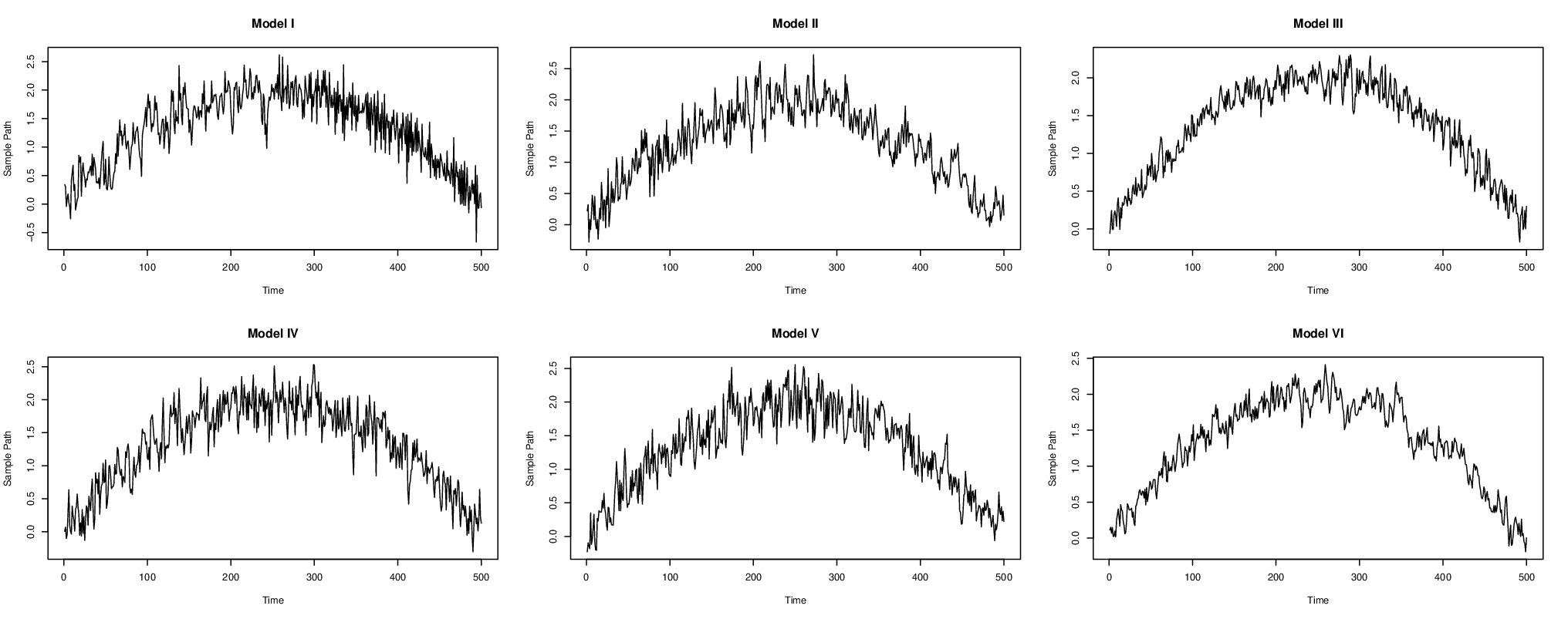
Refer to caption — Figure 1: Typical sample paths of the processes corresponding to model I-VI.

5.1 Change point tests for the variance

In this section we investigate the finite sample properties of the bootstrap tests for the “classical” hypothesis (1.1) of a constant variance and for the null hypothesis (1.3) of a non relevant change in the variance. It turned out that for change point analysis of the variance the Minimal Volatility (MV) method for the selection of the bandwidth provided slightly better results than the commonly used cross validation. The MV-method has been advocated in Politis et al., (1999). To be precise consider a sufficiently wide interval $(a,b)\subset(0,1)$ and define the points $d_{i}:=a+(i-1)(b-a)/l\in(a,b)$ , $i=1,2,\ldots,l$ as potential bandwidths. For each $d_{i}$ , we calculate the statistic $\hat{T}_{n}(i)$ , which is defined as the test statistic $\hat{T}_{n}$ in (3.1) with bandwidth $b_{n}=d_{i}$ . We then calculate for $i=4,\ldots,l-3$ the standard errors $SD(i):=sd(\hat{T}_{n}(j),i-3\leq j\leq i+3)$ of different subsamples of these statistics. Finally, the bandwidth $b_{n}$ in the interval $(a,b)$ is chosen as $b_{n}=d_{i^{*}}$ , where ${i^{*}}=\mathop{\mbox{argmin}}_{4\leq i\leq l-3}SD(i)$ .
In the following we discuss three models for the filters of the innovations in model (2.1).

: (I) $G(t,\mathcal{F}_{i})=H(t,\mathcal{F}_{i})/4$ , where $H(t,\mathcal{F}_{i})=0.5H(t,\mathcal{F}_{i-1})+\varepsilon_{i}$ for $t\leq 0.5$ , and $H(t,\mathcal{F}_{i})=-0.5H(t,\mathcal{F}_{i-1})+\varepsilon_{i}$ for $t>0.5$ .
: (II) $G(t,\mathcal{F}_{i})=H(t,\mathcal{F}_{i})\sqrt{1-a^{2}(t)}/4$ , where $H(t,\mathcal{F}_{i})=\sum_{j=0}^{\infty}a^{j}(t)\varepsilon_{i-j}$ and $a(t)=1/4+t/2$ .
: (III) $G(t,\mathcal{F}_{i})=H(t,\mathcal{F}_{i})\sqrt{1-a^{2}(t)}/8$ for $t\leq 0.5$ , and $G(t,\mathcal{F}_{i})=H(t,\mathcal{F}_{i})\sqrt{2(1-b^{2}(t))}/8$ for $t>0.5$ . Here $H(t,\mathcal{F}_{i})=\sum_{j=0}^{\infty}a^{j}(t)\varepsilon_{i-j}$ for $t\leq 0.5$ , and $H(t,\mathcal{F}_{i})=\sum_{j=0}^{\infty}b^{j}(t)\varepsilon_{i-j}$ for $t>0.5$ , $a(t)=1/4+t/2$ and $b(t)=0.5-(t-0.5)^{2}$ .

Model (I) is a piecewise stationary process. The correlation has a structural break at the point $t=0.5$ . Model (II) is a locally stationary process. The MA coefficient is smoothly time-varying. By our construction, the variance of model (I) and model (II) remains constant, which means that both models correspond to the “classical” null hypothesis in (1.1). Model (III) is a piecewise locally stationary process. The correlation of model (III) has a jump at the point $t=0.5$ . The MA coefficients before and after the point $t=0.5$ are smoothly varying. The variance of model (III) also has a jump at $t=0.5$ and remains constant before and after the jump, respectively. This model corresponds to the null hypothesis in (1.3) of a non relevant change point in the variance. Typical trajectories of the processes corresponding to model (I) - (III) are displayed in the upper part of Figure 1.

Table 1: Simulated Type I error of the tests (3.7) and (4.7) for a change in the variance for various bandwidths and the bandwidth calculated by the MV-method (last line). Left and middle column: test for the hypothesis (1.1) (model (I) and (II)). Right column: test for the hypothesis (1.3) (model (III)).

model	I		II		III
$b_{n}/\alpha$	5%	10%	5%	10%	5%	10%
0.025	19.15	31.55	30.45	44.9	2.45	4.95
0.05	8.8	16.9	15.2	25.9	5.4	8.7
0.075	5.7	13.1	10.25	18.75	7.55	11.9
0.1	6.05	12.8	8.85	16.3	8.15	12.7
0.125	4.75	10.95	7.95	15.2	7.4	12.15
0.15	5.55	11.9	7.3	14.5	8.75	14.05
0.175	4.1	10.2	6.5	14.5	8	13.05
0.2	4.6	10.7	4.9	11.15	7.55	11.8
0.225	3.55	8.85	4.75	10.3	7.3	12.85
0.25	3	8	5.15	10.8	8.35	14.75
0.275	3.05	9.3	4.75	10.7	7.8	14.15
0.3	4.15	9.55	5.6	10.35	16.35	26.65
MV	4.7	11.4	6.75	13.9	6.75	12.3

For model (I) and (II) we investigate approximation of the nominal level of the bootstrap test (3.7) for the classical hypothesis (1.1) of a change in the variance over the interval $[0,1]$ . The corresponding rejection probabilities are displayed in the left and middle column of Table 1. We display the simulated type I error using different bandwidths in the interval $(0.025,0.3)$ and the bandwidth calculated by the MV-method (last line). We observe that the results are rather stable with respect to the choice of $b_{n}$ . Only if $b_{n}\leq 0.1$ the level is overestimated. In particular the bandwidth calculated by the MV-method yields good results for both models.

For model (III), we are interested in testing the hypothesis (1.3) of non relevant changes in variance, where the threshold is given by $\delta=1/64$ . The corresponding rejection probabilities are shown in the right column of Table 1 for the case that $\Delta=\delta=1/64$ . Note that this choice corresponds to the boundary of the null hypothesis, and according to Remark 4.1 the nominal level is smaller in the interior of the null hypothesis, i.e. $\Delta<\delta$ (these results are not displayed for the sake of brevity). Interestingly - compared to the problem of testing the “classical” hypothesis (1.1) - the method is more sensitive with respect to the choice of the bandwidth. However, the MV-method yields a rather accurate approximation of the nominal level.

5.2 Change point tests for a lag $k$ -correlation

We now investigate the same properties of the tests for changes in the lag $1$ -correlation. For this purpose we consider the following models.

: (IV) $G(t,\mathcal{F}_{i})=H(t,\mathcal{F}_{i})\sqrt{1-(t-0.5)^{2}}/4$ , where $H(t,\mathcal{F}_{i})=0.3H(t,\mathcal{F}_{i})+\varepsilon_{i}$ .
: (V) $G(t,\mathcal{F}_{i})=H(t,\mathcal{F}_{i})\sqrt{c(t)}/4$ for $t\leq 0.5$ , and $G(t,\mathcal{F}_{i})=H(t,\mathcal{F}_{i})\sqrt{d(t)}/4$ for $t>0.5$ , where $c(t)=1-(t-0.5)^{2}$ , $d(t)=1-\frac{1}{2}\sin t$ and $H(t,\mathcal{F}_{i})=0.3H(t,\mathcal{F}_{i})+\varepsilon_{i}$ .
: (VI) $G(t,\mathcal{F}_{i})=H(t,\mathcal{F}_{i})\sqrt{1-(t-0.5)^{2}}/8$ , where $H(t,\mathcal{F}_{i})=0.5H(t,\mathcal{F}_{i-1})+\varepsilon_{i}$ for $t\leq 0.5$ , and $H(t,\mathcal{F}_{i})=0.7H(t,\mathcal{F}_{i-1})+\varepsilon_{i}$ for $t>0.5$ .

Model (IV) is a locally stationary processes. The variance of the process is time-varying, but the correlation remains constant. Model (V) and model (VI) are piecewise locally stationary processes, where the variance has a change point. Before and after the jump, the variance varies smoothly. The correlation of model (IV) and (V) is constant, while the correlation of model (VI) has a break at $t=0.5$ . Typical trajectories corresponding to these processes are depicted in the lower part of Figure 1

Note that the change point analysis by the tests proposed in Section 4.1 and 4.2 requires the choice of two bandwidths in the local linear estimates of the mean and variance. We use a generalized cross validation method introduced by Zhou and Wu, (2010) to select the bandwidth for estimating the mean function. Then we apply this cross validation procedure again to select the bandwidth for estimating the variance function. The parameters $L$ and $\zeta$ in the estimator (3.10) are chosen as $L=\lfloor n^{1/3}\rfloor$ and $\zeta=0.016$ , respectively.

The corresponding rejection probabilities are displayed in Table 2 for various bandwidths $b_{n}$ in the interval $(0.025,0.3)$ . At each fixed $b_{n}$ , the bandwidth for variance $c_{n}$ is calculated by cross validation. The results for the bandwidths calculated by cross validation are displayed in the last row of the table. The left and middle column correspond to the “classical” hypothesis whether the correlation remains constant (model (IV) and (V)). We observe a very accurate approximation of the nominal level if the bandwidth is chosen such that $b_{n}<0.1$ . If $b_{n}\in(0.1,0.3)$ the nominal level is slightly underestimated. For both models the generalized cross validation proposed by Zhou and Wu, (2010) yields a rather accurate approximation of the nominal level,

The right column of Table 2 shows the simulated type I error of the test (4.10) for a non relevant change in correlation with $\delta=0.2$ . Again the case $\delta=\Delta=0.2$ is displayed in model (VI) corresponding to the boundary of the null hypothesis, and the simulated rejection probabilities are smaller if $|\Delta|<\delta$ . Compared to the test for a non relevant change in the variance (see Table 1) the test for a non relevant change in the correlation is rather stable with respect to the choice of the bandwidth. Also the proposed cross validation methodology performs reasonably well, which is reported in the last line of Table 2.

Table 2: Simulated Type I error of the tests for a change in the lag

1

-correlation for various bandwidths and the bandwidth calculated by generalized cross validation (last line). Left and middle column: test for the hypothesis (3.8) (model (IV) and (V)). Right column: test for the hypothesis (4.10) (model (VI)).

model	IV		V		VI
$b_{n}/\alpha$	5%	10%	5%	10%	5%	10%
0.025	4.7	10.4	4.9	10.3	6	8.95
0.05	3.75	8.5	4.5	9.1	6	9.25
0.075	4.15	9.7	4.4	9.6	7.05	9.9
0.1	3.4	8.1	3.4	8.1	6.05	9.55
0.125	3.85	9.1	4.05	8.25	6.4	9.35
0.15	3.35	8.35	3.2	8.25	5.3	7.7
0.175	2.85	8.15	3.5	8.3	4.9	6.75
0.2	2.6	7.6	3.95	8.9	4.5	6.95
0.225	2.9	7.75	3.1	8.05	4	6
0.25	3.1	8	3.45	8.25	5.15	7.6
0.275	2.8	8.75	3.5	8.9	6.3	8.9
0.3	3.05	8.55	3.15	8.35	5.9	8.8
CV	5	10.15	4.75	9.65	6.75	10.45

Finally, we display in Figure 2 the simulated rejection probabilities of the tests for the hypotheses (1.3) and (4.10) for a non relevant change in the variance or correlation, respectively, as a function of the parameter $\delta\in[0,2\Delta]$ . The significance level is chosen as $0.1$ . As expected the probability of rejection decreases with $\delta$ (see also the discussion in Remark 4.1).

5.3 Power properties

In this section we investigate the power of the tests proposed in this paper considering the following four scenarios.

: (I’) $G(t,\mathcal{F}_{i})=(\mathbf{1}(t\leq 0.5)+\mathbf{1}(t>0.5)\sqrt{1+\lambda})H(t,\mathcal{F}_{i})/4$ , where $\lambda>-1$ , $H(t,\mathcal{F}_{i})=0.5H(t,\mathcal{F}_{i-1})+\varepsilon_{i}$ for $t\leq 0.5$ , and $H(t,\mathcal{F}_{i})=-0.5H(t,\mathcal{F}_{i-1})+\varepsilon_{i}$ for $t>0.5$ .
: (II’) $G(t,\mathcal{F}_{i})=H(t,\mathcal{F}_{i})\big[\mathbf{1}(t\leq 0.5)\sqrt{1-a^{2}(t)}+\mathbf{1}(t>0.5)\sqrt{(2+\lambda)(1-b^{2}(t))}\big]/8$ , where $H(t,\mathcal{F}_{i})=\sum_{j=0}^{\infty}a^{j}(t)\varepsilon_{i-j}$ for $t\leq 0.5$ , and $H(t,\mathcal{F}_{i})=\sum_{j=0}^{\infty}b^{j}(t)\varepsilon_{i-j}$ for $t>0.5$ and the function $a$ and $b$ are defined by $a(t)=1/4+t/2$ and $b(t)=0.5-(t-0.5)^{2}$ , respectively.
: (III’) $G(t,\mathcal{F}_{i})=\sqrt{1-(t-0.5)^{2}}/4H(t,\mathcal{F}_{i})$ , where $H(t,\mathcal{F}_{i})=0.3H(t,\mathcal{F}_{i})+\varepsilon$ for $t\leq 0.5$ , and $H(t,\mathcal{F}_{i})=(0.3-\lambda)H(t,\mathcal{F}_{i})+\varepsilon$ for $t>0.5$ .
: (IV’) $G(t,\mathcal{F}_{i})=H(t,\mathcal{F}_{i})\sqrt{1-(t-0.5)^{2}}/8$ , where $H(t,\mathcal{F}_{i})=(0.5-\lambda)H(t,\mathcal{F}_{i-1})+\varepsilon_{i}$ for $t\leq 0.5$ , and $H(t,\mathcal{F}_{i})=0.7H(t,\mathcal{F}_{i-1})+\varepsilon_{i}$ for $t>0.5$ ,

Model (I’) is used to study the power of the test (3.7) where the case $\lambda=0$ corresponds to the null hypothesis of a constant variance. The power properties of the test (4.7) for a non relevant change in the variance is investigated in model (II’). Here we test the hypotheses $H_{0}:\Delta\leq 1/64$ versus $H_{1}:\Delta>1/64$ , where the case $-2<\lambda\leq 0$ corresponds to the null hypothesis. Similarly, the power of the test for a constant lag $1$ -correlation (3.18) is studied in model (III’) (again the case $\lambda=0$ corresponds to the null hypothesis of a constant correlation) and the corresponding hypotheses $H_{0}:\Delta\leq 0.2$ versus $H_{1}:\Delta>0.2$ of a non relevant change in the lag $1$ -correlation are investigated in model (IV’) (here the case $-0.4\leq\lambda\leq 0$ corresponds to the null hypothesis). The rejection probabilities for various values of $\lambda$ are displayed in Figure 3. We observe that the proposed methodology can detect (relevant) changes in the variance or correlation with reasonable size.

6 Data Analysis

Various scientific data show that since the late 1800s, the mean global temperature starts to increase significantly. For example, during 1906–2005, the Earth’s average surface temperature rose by $0.74\pm 0.18$ ^∘C, with the rate of warming also increasing with time. On the other hand, however, there are much fewer studies on possible changes in the second order characteristics (especially the correlations) of temperature time series, both globally and regionally. In this section, we are interested in identifying possible changes in the second order structures of regional temperature in the recent three centuries. To this end, we analyse the Hadley Centre Central England Temperature (HadCET) data from 1659–2015. These data can be downloaded from http://www.metoffice.gov.uk/hadobs/hadcet/. We present the analysis results of monthly temperature series in January and July as representatives of the winter and summer monthly temperature patterns in central England. The time series are shown in Figure 4. There are apparent increasing trends in both time series.

We first test the constancy in the variance and lag $1$ -correlation for the January data. In our analysis the critical values are generated by $8000$ bootstrap replications. The bandwidths were chosen as described in Section 5. The results are summarized in Table 3. The test (3.7) rejects the null hypothesis of no change point in the variance at $5\%$ level. We then use the statistic (4.1) to estimate the change point and obtain $\tilde{t}_{n}=226$ , which corresponds to the year of $1884$ . Next we apply the test (3.7) again to the periods before and after the identified change point and conclude that there are no further structural breaks in the variance during the two periods. The estimates of the variance before and after the year $1884$ are given by $4.05$ and $2.85$ , respectively. Next we apply (3.18) to testing the constancy in the lag $1$ -correlation, where we use the statistic (3.10) to estimate the change points in the variance with $\zeta=0.14$ and $L=38$ . We identify $t^{*}_{n}=242$ , which corresponds to the year of $1900$ . The result is close to the one which is obtained by the estimator (4.1). The null hypothesis of no change points in the lag $1$ -correlation is rejected at $5\%$ level [see Table 3]. Next we use the statistic (4.12) to identify the location of the change point of the first order correlation and obtain $\hat{t}_{n}=213$ , which corresponds to the year of $1871$ . Again we investigate the existence of further changes in the lag $1$ -correlation before and after the year $1871$ and conclude that there are no further structural breaks in the lag $1$ -correlation during the two periods. The estimates of the lag $1$ -correlation before and after the break point are equal to $-0.108$ and $0.231$ , respectively.

The results from Section 4 enable us to perform tests for relevant changes in the variance and lag $1$ -correlation for the January data. Figure 5 displays the $p$ -values of the tests for a relevant change in the variance and log $1$ -correlation for different values of the threshold $\delta$ . At the 5% significance level, we conclude that there exists a relevant change with size $\delta=0.645$ in the variance and a relevant change with size $\delta=0.313$ in the lag $1$ -correlation.

For comparison, we also analyse the July data. For the variance, we choose the bandwidths $b_{n}=0.205$ and $m=33$ . The test statistic (3.1) is 1.90, together with the simulated $90\%$ critical value 1.83 and $95\%$ critical value 2.04. Hence we cannot reject the null hypothesis of no change point in the variance at the $5\%$ significance level. For the correlation, the bandwidths are chosen as $b_{n}=0.26$ , $c_{n}=0.06$ and $m=25$ . The test statistic (3.14) is 0.84, and the simulated $90\%$ critical value is 1.11, and the $95\%$ critical value is 1.25. Hence, again we cannot reject the null hypothesis of no change points in lag $1$ -correlation at the $10\%$ significance level.

In conclusion, our data analysis suggests that besides the mean trend, there exists strong evidence indicating structural changes in the second order structures of monthly temperatures in central England. Further, the latter changes are inhomogeneous among different seasons, in the sense that changes in the variance and correlation are more significant in the winter than in the summer. This implies that winter temperatures in central England have become more unstable and more difficult to predict since the late 19th century. Finally, we also locate the change point in the second order structure of the HadCET temperate data through all three ways we proposed in our paper. The three change points, $1871$ , $1884$ and $1900$ , are quite close. Our findings suggest that the time of change in the second order structure of our data coincides with that of the mean global temperature identified in various previous studies.

Table 3: Tests for the existence of a change point in the variance and lag

1

-correlation in the HadCET data.

v^{*}_{\alpha}

denotes the critical values obtained by the bootstrap procedure. “Whole” represents the whole period, “Before” and “After” represent the period before and after the detected change point, respectively.

	Variance			lag $1$ -Correlation
	Whole	Before	After	Whole	Before	After
Test Stat.	5.29**	2.82	3.34	1.53**	0.64	0.71
$v^{*}_{90\%}$	4.56	4.66	5.1	1.31	0.76	0.95
$v^{*}_{95\%}$	5.11	5.22	5.67	1.45	0.85	1.07
$b_{n}$	0.155	0.26	0.26	0.23	0.19	0.21
$m$	40	30	18	19	32	11
$c_{n}$	–	–	–	0.05	0.06	0.059

Acknowledgements. The work of H. Dette has been supported in part by the Collaborative Research Center “Statistical modeling of nonlinear dynamic processes” (SFB 823, Teilprojekt A1, C1) of the German Research Foundation (DFG). Z. Zhou’s research has been supported in part by NSERC of Canada. The authors would like to thank Martina Stein who typed this manuscript with considerable technical expertise.

References

Abraham and Wei, (1984) Abraham, B. and Wei, W. W. S. (1984). Inferences about the parameters of a time series model with changing variance. Metrika, 31:183–194.
Andrews, (1993) Andrews, D. W. K. (1993). Tests for parameter instability and structural change with unknown change point. Econometrica, 61(4):128–156.
Aue et al., (2009) Aue, A., Hörmann, S., Horváth, L., and Reimherr, M. (2009). Break detection in the covariance structure of multivariate time series models. Annals of Statistics, 37(6):4046–4087.
Aue and Horváth, (2013) Aue, A. and Horváth, L. (2013). Structural breaks in time series. Journal of Time Series Analysis, 34(1):1–16.
Baufays and Rasson, (1985) Baufays, P. and Rasson, J. P. (1985). Variance changes in autoregressive models. In Anderson, D., editor, Time Series Analysis: Theory and Practice 7, pages 119–127. North-Holland, New York.
Berger and Delampady, (1987) Berger, J. O. and Delampady, M. (1987). Testing precise hypotheses. Statistical Science, 2(3):317–335.
Berkson, (1938) Berkson, J. (1938). Some difficulties of interpretation encountered in the application of the chi-square test. Journal of the American Statistical Association, 33(203):526–536.
Chen and Gupta, (1997) Chen, J. and Gupta, A. K. (1997). Testing and locating variance changepoints with application to stock prices. Journal of the American Statistical Association, 92(438):739–747.
Chow and Liu, (1992) Chow, S.-C. and Liu, P.-J. (1992). Design and Analysis of Bioavailability and Bioequivalence Studies. Marcel Dekker, New York.
Davis et al., (2006) Davis, R. A., Lee, T. C. M., and Rodriguez-Yam, G. A. (2006). Structural break estimation for nonstationary time series models. Journal of the American Statistical Association, 101(473):223–239.
Dette and Wied, (2014) Dette, H. and Wied, D. (2014). Detecting relevant changes in time series models. Journal of the Royal Statistical Society, Ser., B., to appear, arxiv.org/abs/1403.8120 .
Fan and Gijbels, (1996) Fan, J. and Gijbels, I. (1996). Local Polynomial Modelling and its Applications. Chapman & Hall, London.
Galeano and Peña, (2007) Galeano, P. and Peña, D. (2007). Covariance changes detection in multivariate time series. Journal of Statistical Planning and Inference, 137:194–211.
Inclán and Tiao, (1994) Inclán, C. and Tiao, G. C. (1994). Use of cumulative sums of squares for retrospective detection of changes of variance. Journal of the American Statistical Association, 89(427).
Jandhyala et al., (2013) Jandhyala, V., Fotopoulos, S., MacNeill, I., and Liu, P. (2013). Inference for single and multiple change-points in time series. Journal of Time Series Analysis, 34(4):423–446.
Lee and Park, (2001) Lee, S. and Park, S. (2001). The cusum of squares test for scale changes in infinite order moving average processes. Scandinavian Journal of Statistics, 28(4):625644.
Mallik et al., (2013) Mallik, A., Banerjee, M., and Sen, B. (2013). Asymptotics for $p$ -value based threshold estimation in regression settings. Electronic Journal of Statistics, 7:2477–2515.
Mallik et al., (2011) Mallik, A., Sen, B., Banerjee, M., and Michailidis, G. (2011). Threshold estimation based on a p-value framework in dose-response and regression settings. Biometrika, 98:887–900.
Mcbride, (1999) McBride, G. B. (1999). Equivalence tests can enhance environmental science and management. Australian $\&$ New Zealand Journal of Statistics, 41:19–29.
Müller, (1992) Müller, H.-G. (1992). Change-points in nonparametric regression analysis. Annals of Statistics, 20:737–761.
Page, (1954) Page, E. S. (1954). Continuous inspection schemes. Biometrika, 41:100–115.
Politis et al., (1999) Politis, D. N., Romano, J. P., and Wolf, M. (1999). Subsampling. Springer, New York.
Preuss et al., (2014) Preuss, P., Puchstein, R., and Dette, H. (2014). Detection of multiple structural breaks in multivariate time series. Journal of the American Statistical Association, DOI: 10.1080/01621459.2014.920613.
Qu, (2008) Qu, Z. (2008). Testing for structural change in regression quantiles. Journal of Econometrics, 148:170–184.
Solomon, (2007) Solomon, S. (2007). Climate change 2007-the physical science basis: Working group I contribution to the fourth assessment report of the IPCC, volume 4. Cambridge University Press.
Vogt, (2012) Vogt, M. (2012). Nonparametric regression for locally stationary time series. The Annals of Statistics, 40(5):2601–2633.
Vogt and Dette, (2015) Vogt, M. and Dette, H. (2015). Detecting gradual changes in locally stationary processes. Annals of Statistics, 43(2):713–740.
Wichern et al., (1976) Wichern, D. W., Miller, R. B., and Hsu, D.-A. (1976). Changes of variance in first-order autoregressive time series models - with an application. Journal of the Royal Statistical Society. Ser. C (Applied Statistics), 25(3):248–256.
Wied et al., (2012) Wied, D., Krämer, W., and Dehling, H. (2012). Testing for a change in correlation at an unknown point in time using an extended functional delta method. Econometric Theory, 28(3):570–589.
Wu, (2005) Wu, W. B. (2005). Nonlinear system theory: Another look at dependence. Proceedings of the National Academy of Sciences of the United States of America, 102(40):14150–14154.
Zhou, (2013) Zhou, Z. (2013). Heteroscedasticity and autocorrelation robust structural change detection. Journal of the American Statistical Association, 108:726–740.
Zhou, (2014) Zhou, Z. (2014). Inference of weighted $V$ -statistics for non-stationary time series and its applications.. Annals of Statistics, 42:87–114.
Zhou and Wu, (2010) Zhou, Z. and Wu, W. B. (2010). Simultaneous inference of linear models with time-varying coefficients. Journal of the Royal Statistical Society, Series B, 72:513–531.

7 Proofs of main results

In this section we provide proofs of the main results, where some of the technical details are deferred to an online supplement. Throughout this section the symbol $\Rightarrow$ denotes weak convergence of a stochastic process in $\mathcal{C}(0,1)$ with the uniform topology.

7.1 Proof of Theorem 3.1, 3.2, Lemma 3.1, Theorem 3.3 and 3.4

7.1.1 Proof of Theorem 3.1

In order to study the asymptotic properties of the statistic $\hat{T}_{n}$ we introduce the random variable

\displaystyle T_{n}=\max_{1\leq i\leq n}\Big|S_{i}-\frac{i}{n}S_{n}\Big|,

where $S_{i}$ is the $i$ th partial sum of the PLS $\{e_{i}^{2}\}_{i=1}^{n}$ , that is $S_{i}=\sum_{j=1}^{i}e_{j}^{2}$ . It follows from the results of Zhou, (2013) that $\frac{1}{\sqrt{n}}T_{n}\stackrel{{\scriptstyle\cal D}}{{\longrightarrow}}\sup_{t\in(0,1)}|U_{1}(t)-tU_{1}(1)|$ , where $\{U_{1}(t)\}_{t\in[0,1]}$ is a centered Gaussian process with covariance kernel (3.5).

We will show below that for the maximum deviation between $\hat{S}_{i}$ and $S_{i}$ satisfies

\max_{1\leq i\leq n}|S_{i}-\hat{S}_{i}|=O_{p}(\sqrt{nb_{n}}+nb_{n}^{3}+b_{n}^{-1}).

(7.1)

From (7.1) we obtain $T_{n}-\hat{T}_{n}=O_{p}(\sqrt{nb_{n}}+nb_{n}^{3}+b_{n}^{-1})=o(\sqrt{n})$ , where the last estimate follows from our choice of the bandwidth $b_{n}$ . This yields the assertion of Theorem 3.1.

For a proof of the remaining estimate (7.1) we use the decomposition

\displaystyle{S}_{i}-\hat{S}_{i}=A_{n,i}+B_{n,i},

(7.2)

where the quantities $A_{n,i}$ and $B_{n,i}$ are defined by

\displaystyle A_{n,i}=2\sum_{j=1}^{i}e_{j}\big(\hat{\mu}_{b_{n}}(t_{j})-\mu(t_{j})\big),\quad B_{n,i}=\sum_{j=1}^{i}\big(\mu(t_{j})-\hat{\mu}_{b_{n}}(t_{j})\big)^{2}.

Observing the estimate (8.4) in Section 8.1 of the technical appendix we have $0\leq B_{n,i}\leq B_{n,n}=O_{p}(b_{n}^{-1}+nb_{n}^{4})$ for all $1\leq i\leq n$ , which implies

\displaystyle\max_{1\leq i\leq n}B_{n,i}=O_{p}(b_{n}^{-1}+nb_{n}^{4}).

(7.3)

By Lemma 8.1 (which is proved in Section 8.1) it follows that

		$\displaystyle\max_{{\lfloor nb_{n}\rfloor}\leq i\leq n-\lfloor nb_{n}\rfloor}\Big\|A_{n,i}-2\sum_{j=\lfloor nb_{n}\rfloor+1}^{i}a_{n,j}-2\sum_{j=1}^{\lfloor nb_{n}\rfloor}e_{j}(\hat{\mu}_{b_{n}}(t_{j})-\mu(t_{j}))\Big\|=O_{p}(n\chi_{n}),$
		$\displaystyle\max_{n-\lfloor nb_{n}\rfloor+1\leq i\leq n}\Big\|A_{n,i}-2\sum_{j=\lfloor nb_{n}\rfloor}^{n-\lfloor nb_{n}\rfloor}a_{n,j}-2\sum_{j=1}^{\lfloor nb_{n}\rfloor-1}e_{j}(\hat{\mu}_{b_{n}}(t_{j})-\mu(t_{j}))$
		$\displaystyle\qquad\qquad\qquad\qquad\qquad\qquad-2\sum_{j=n-\lfloor nb_{n}\rfloor+1}^{{i}}e_{j}(\hat{\mu}_{b_{n}}(t_{j})-\mu(t_{j}))\Big\|=O_{p}(n\chi_{n}),$

where $\chi_{n}=b_{n}^{3}+\frac{b_{n}}{n}$ , and

\displaystyle a_{n,j}=\frac{e_{j}}{nb_{n}}\sum^{n}_{s=1}K_{b_{n}}\big(\frac{s-j}{n}\big)e_{s}\qquad(j=1,\dots,n).

(7.4)

A further application of the estimate (8.4) in Section 8.1 and the Cauchy-Schwarz inequality gives

$\displaystyle\Big\\|\max_{1\leq j\leq\lfloor nb_{n}\rfloor}\Big\|\sum_{i=1}^{j}e_{j}\big(\mu(t_{j})-\hat{\mu}_{b_{n}}(t_{j})\big)\Big\|\Big\\|_{2}$	$\displaystyle\leq$	$\displaystyle\sum_{i=1}^{\lfloor nb_{n}\rfloor}\\|e_{j}\\|_{4}\\|\mu(t_{j})-\hat{\mu}_{b_{n}}(t_{j})\\|_{4}$
	$\displaystyle=$	$\displaystyle O(\sqrt{nb_{n}}+nb_{n}^{3}),$
$\displaystyle\Big\\|\max_{n-\lfloor nb_{n}\rfloor+1\leq j\leq n}\Big\|\sum_{i={n-\lfloor nb_{n}\rfloor+1}}^{j}e_{j}\big(\mu(t_{j})-\hat{\mu}_{b_{n}}(t_{j})\big)\Big\|\Big\\|_{2}$	$\displaystyle=$	$\displaystyle O(\sqrt{nb_{n}}+nb_{n}^{3}).$

This implies that

\max_{1\leq i\leq n}|A_{n,i}|\leq\max_{\lfloor nb_{n}\rfloor\leq i\leq n-\lfloor nb_{n}\rfloor}|\bar{A}_{n,i}|+O_{p}(\sqrt{nb_{n}}+nb^{3}_{n}),

(7.5)

where $\bar{A}_{n,i}=2\sum^{i}_{j=\lfloor nb_{n}\rfloor}a_{n,j}$ and $a_{n,j}$ is defined in (7.4).

In the following we derive an estimate for the first term on the right-hand side of (7.5). For this purpose we consider the random variables $\tilde{e}_{s,m}=\mathbb{E}(e_{s}|\varepsilon_{s},...,\varepsilon_{s-m})$ and note that the sequence $(\tilde{e}_{s,m})^{n}_{s=1}$ is $m$ -dependent. Now define $a^{(m)}_{n,j}=e_{j}\sum_{s=1}^{n}K_{b_{n}}\big(\frac{s-j}{n}\big)\tilde{e}_{s,m}/(nb_{n})$ and

\displaystyle\bar{A}^{(m)}_{n,i}=2\sum_{j=\lfloor nb_{n}\rfloor}^{i}a^{(m)}_{n,j},

then a similar argument as given in the proof of Theorem 1 of Zhou, (2014) shows that

\displaystyle\max_{1\leq j\leq n}\Big\|\sum_{s=1}^{n}K_{b_{n}}\big(\frac{s-j}{n}\big)(\tilde{e}_{s,m}-e_{s})\Big\|_{4}\leq C\sqrt{nb_{n}}m\chi^{m}

for some constant $\chi\in(0,1)$ . By the Cauchy-Schwartz inequality it follows that

	$\displaystyle\Big\\|\max_{\lfloor nb_{n}\rfloor\leq i\leq n-\lfloor nb_{n}\rfloor}\|\bar{A}_{n,i}-\bar{A}^{(m)}_{n,i}\|\Big\\|_{2}$	$\displaystyle\leq$	$\displaystyle\Big\\|\frac{2}{nb_{n}}\sum_{j=\lfloor nb_{n}\rfloor}^{n-\lfloor nb_{n}\rfloor}\|e_{j}\|\sum_{s=1}^{n}K_{b_{n}}\big(\frac{s-j}{n}\big)(\tilde{e}_{s,m}-e_{s})\|\Big\\|_{2}$		(7.6)
		$\displaystyle=$	$\displaystyle O(\sqrt{n}m\chi^{m}b_{n}^{-1/2}).$		(7.6)

With the notations $\tilde{a}^{(m)}_{n,j}=\tilde{e}_{j,m}\sum_{s=1}^{n}K_{b_{n}}(\frac{s-j}{n})\tilde{e}_{s,m}/(nb_{n})$ and $\tilde{A}^{(m)}_{n,i}=2\sum_{j=\lfloor nb_{n}\rfloor}^{i}\tilde{a}^{(m)}_{n,j}$ it is easy to see that

\displaystyle\Big\|\max_{\lfloor nb_{n}\rfloor\leq i\leq n-\lfloor nb_{n}\rfloor}|\tilde{A}^{(m)}_{n,i}-\bar{A}^{(m)}_{n,i}|\Big\|_{2}\leq\frac{2}{nb_{n}}\sum_{j=1}^{n}\|e_{j}-\tilde{e}_{j,m}\|_{4}\Big\|\sum_{s=1}^{n}K_{b_{n}}(\frac{s-j}{n})\tilde{e}_{s,m}\Big\|_{4}.

(7.7)

Now an elementary calculation via Burkholder’s inequality shows

\displaystyle\max_{1\leq j\leq n}\Big\|\frac{1}{nb_{n}}\sum_{s=1}^{n}K_{b_{n}}\Big(\frac{s-j}{n}\Big)\tilde{e}_{s,m}\Big\|_{4}=O\Big(\frac{1}{\sqrt{nb_{n}}}\Big),

and by a similar argument as given in the proof of Theorem 1 of Zhou, (2014) we have for some constant $\chi\in(0,1)$ the estimate $\max_{1\leq j\leq n}\|\tilde{e}_{j,m}-e_{j}\|_{4}=O(\chi^{m})$ . This gives for the left-hand side of (7.7)

\displaystyle\Big\|\max_{\lfloor nb_{n}\rfloor\leq i\leq n-\lfloor nb_{n}\rfloor}|\bar{A}^{(m)}_{n,i}-\tilde{A}^{(m)}_{n,i}|\Big\|_{2}=O(\sqrt{n/b_{n}}\chi^{m}),

and an application of (7.6) yields

\displaystyle\Big\|\max_{\lfloor nb_{n}\rfloor\leq i\leq n-\lfloor nb_{n}\rfloor}|\bar{A}_{n,i}-\tilde{A}^{(m)}_{n,i}|\Big\|_{2}=O(\sqrt{n/b_{n}}m\chi^{m}).

(7.8)

A tedious but straightforward calculation shows that $\mathcal{P}_{j-l}(\tilde{e}_{j,m}\tilde{e}_{i,m})=0$ for $l>2m$ . For example, if $i\geq j-m$ , then by definition, $\tilde{e}_{j,m}\tilde{e}_{i,m}$ is $\sigma(\varepsilon_{j-2m},\varepsilon_{j-2m+1},...,\varepsilon_{i})$ measurable. Consequently, $\mathbb{E}(\tilde{e}_{j,m}\tilde{e}_{i,m}|\mathcal{F}_{j-l})=\mathbb{E}(\tilde{e}_{j,m}\tilde{e}_{i,m}|\mathcal{F}_{j-l-1})=\mathbb{E}(\tilde{e}_{j,m}\tilde{e}_{i,m})$ if $l>2m$ , which gives $\mathcal{P}_{j-l}(\tilde{e}_{j,m}\tilde{e}_{i,m})=0$ . The other cases $i\leq j-l-1$ and $j-l\leq i\leq j-m-1$ are treated similarly, and details are omitted for the sake of brevity. Observing $\mathcal{P}_{j-l}(\tilde{e}_{j,m}\tilde{e}_{i,m})=0$ for $l>2m$ we obtain

\displaystyle\Big\|\max_{\lfloor nb_{n}\rfloor\leq i\leq n-\lfloor nb_{n}\rfloor}|\tilde{A}^{(m)}_{n,i}-\mathbb{E}\tilde{A}^{(m)}_{n,i}|\Big\|_{2}\leq{2}\sum_{l=0}^{2m}\Big\|\max_{\lfloor nb_{n}\rfloor\leq i\leq n-\lfloor nb_{n}\rfloor}|\sum_{j=\lfloor nb_{n}\rfloor}^{i}\mathcal{P}_{j-l}\tilde{a}^{(m)}_{n,j}|\Big\|_{2}.

(7.9)

Similar arguments as given in the proof of Theorem 1 in Wu, (2005) show

\displaystyle\|\mathcal{P}_{j-l}\tilde{a}^{(m)}_{n,j}\|_{2}\leq\frac{M}{n}\Big\|\tilde{e}_{j,m}\sum_{s=1}^{n}\tilde{e}_{s,m}K_{b_{n}}\Big(\frac{s-j}{n}\Big)-\tilde{e}^{(j-l)}_{j,m}\sum_{s=1}^{n}\tilde{e}^{(j-l)}_{s,m}K_{b_{n}}\Big(\frac{s-j}{n}\Big)\Big\|_{2},

and by the triangle inequality it follows that

\displaystyle\|\mathcal{P}_{j-l}\tilde{a}^{(m)}_{n,j}\|_{2}\leq M(Z_{1,j}+Z_{2,j}),

where the terms $Z_{1,j}$ and $Z_{2,j}$ are defined by

	$\displaystyle Z_{1,j}$	$\displaystyle=\frac{1}{nb_{n}}\Big\\|\tilde{e}_{j,m}\sum_{s=1}^{n}K_{b_{n}}\Big(\frac{s-j}{n}\Big)\big[\tilde{e}_{s,m}^{(j-l)}-\tilde{e}_{s,m}\big]\Big\\|_{2},$
	$\displaystyle Z_{2,j}$	$\displaystyle=\frac{1}{nb_{n}}\Big\\|\big[\tilde{e}^{(j-l)}_{j,m}-\tilde{e}_{j,m}\big]\sum_{s=1}^{n}K_{b_{n}}\Big(\frac{s-j}{n}\Big)\tilde{e}^{(j-l)}_{s,m}\Big\\|_{2},$

$\tilde{e}_{s,m}^{(j)}=\mathbb{E}(e_{s}^{(j)}|\varepsilon_{s-m},\ldots,\varepsilon_{j}^{\prime},\ldots,\varepsilon_{s})$ for $s-m\leq j\leq s$ , $e_{s}^{(j)}=G_{l}(t_{s},\mathcal{F}_{s}^{(j)})$ for $b_{l}<t_{s}\leq b_{l+1}$ and we use the convention $\tilde{e}_{s,m}^{(j)}=\tilde{e}_{s,m}$ for $j<s-m$ or $j>s$ . Elementary calculations show that for $l\geq 0$

\displaystyle\Big\|\sum_{s=1}^{n}K_{b_{n}}(\frac{s-j}{n})\tilde{e}^{(j-l)}_{s,m}\Big\|_{4}=O(\sqrt{nb_{n}}),\qquad 1\leq j\leq n,

while by definition $\|\tilde{e}_{j,m}^{(j-l)}-\tilde{e}_{j,m}\|_{4}=0$ for $l>m$ . On the other hand, if $1\leq j\leq n$ , $0\leq l\leq m$ , we have by Assumption (A4)

\displaystyle\|\tilde{e}_{j,m}^{(j-l)}-\tilde{e}_{j,m}\|_{4}=\big\|\mathbb{E}(e_{j}-e_{j}^{(j-l)}|\varepsilon_{j-m},...,\varepsilon_{j-l},\varepsilon_{j-l}^{\prime},\varepsilon_{j})\big\|_{4}\leq M\chi^{l},

which gives $Z_{2,j}=O(\frac{\chi^{l}}{\sqrt{nb_{n}}})$ . Observing that $\tilde{e}_{s,m}^{(j-l)}-\tilde{e}_{s,m}=0$ if $s\geq j-l+m+1$ or $s\leq j-l-1$ , it is easy to see that $Z_{1,j}=O(\frac{m}{nb_{n}})$ . It now follows from Doob’s inequality

\displaystyle\Big\|\max_{\lfloor nb_{n}\rfloor\leq i\leq n-\lfloor nb_{n}\rfloor}|\sum_{j=\lfloor nb_{n}\rfloor}^{i}\mathcal{P}_{j-l}\tilde{a}^{(m)}_{n,j}|\Big\|_{2}=O\Big(\sqrt{n}\Big(\frac{\chi^{l}}{\sqrt{nb_{n}}}+\frac{m}{nb_{n}}\Big)\Big),

and we obtain from (7.9) that

\displaystyle\Big\|\max_{\lfloor nb_{n}\rfloor\leq i\leq n-\lfloor nb_{n}\rfloor}|\tilde{A}^{(m)}_{n,i}-\mathbb{E}\tilde{A}^{(m)}_{n,i}|\Big\|_{2}=O\Big(\frac{m^{2}}{n^{1/2}b_{n}}+(b_{n})^{-1/2}\Big).

(7.10)

Finally, similar arguments as given in the proof of Lemma 5 in Zhou and Wu, (2010) show

\max_{\lfloor nb_{n}\rfloor\leq i\leq n-\lfloor nb_{n}\rfloor}\mathbb{E}[\tilde{A}_{i,m}]=O\Big(\sum_{i=1}^{n}\sum_{j=1}^{n}\chi^{|i-j|}/(nb_{n})\Big)=O(b_{n}^{-1}).

Observing (7.5), (7.8) and (7.10) and taking $m=M\log n$ for a sufficiently large constant $M>0$ yields $\max_{1\leq i\leq n}|A_{n,i}|=O_{p}(\sqrt{nb_{n}}+nb_{n}^{3}+b_{n}^{-1}).$ Consequently, the assertion (7.1) follows from (7.2), (7.3) and this estimate.

7.1.2 Proof of Theorem 3.2

We recall the definition of $\hat{\Phi}_{i,n}$ in (3.6) and define on the interval $[0,1]$ the linear interpolation

\displaystyle\hat{\tilde{\Phi}}_{m,n}(t)=\hat{\Phi}_{\lfloor nt\rfloor,m}+(nt-\lfloor nt\rfloor)(\hat{\Phi}_{\lfloor nt\rfloor+1,m}-\hat{\Phi}_{\lfloor nt\rfloor,m}).

(7.11)

The assertion follows if the weak convergence

\{\hat{\tilde{\Phi}}_{m,n}(t)\}_{t\in[0,1]}\Rightarrow\{U_{1}(t)\}_{t\in[0,1]}

conditional on $\mathcal{F}_{n}$ can be established. For a proof of this statement define ${\Phi}_{i,m}$ and $\tilde{\Phi}_{m,n}(t)$ by replacing the nonparametric residuals $\{\hat{e}_{i}\}_{i=1}^{n}$ by the (non-observable) errors $\{e_{i}\}_{i=1}^{n}$ in the definition (3.6) and (7.11) of ${\hat{\Phi}}_{i,m}$ and ${\hat{\tilde{\Phi}}}_{m,n}(t)$ , respectively. Note that similar arguments as given in the proof of Theorem 3 in Zhou, (2013) show that { $\tilde{\Phi}_{m,n}(t)\}_{t\in[0,1]}\Rightarrow\{U_{1}(t)\}_{t\in[0,1]}$ . The assertion of Theorem 3.2 then follows from the estimate

\displaystyle\sup_{t\in[0,1]}\big|\tilde{\Phi}_{m,n}(t)-\hat{\tilde{\Phi}}_{m,n}(t)\big|=O_{p}\Bigl(\Bigl(\frac{m\log^{2}n}{nb_{n}^{3/2}}\Bigr)^{1/2}+\sqrt{m}b_{n}^{2}\log n\Bigr).

(7.12)

In order to prove (7.12) let $C$ denote a sufficiently large constant, which may vary from line to line in the following calculations, and consider the event

A_{n}=\Big\{\sup_{t\in[0,1]}|\hat{\mu}_{b_{n}}(t)-\mu(t)|\leq C\Big(\frac{\log n}{\sqrt{nb_{n}}b_{n}^{1/4}}+b_{n}^{2}\log n\Big)\Big\}.

By Lemma 8.3 of Section 8.1 in the technical appendix we have that $\lim_{n\rightarrow\infty}\mathbb{P}(A_{n})=1$ . This yields for $1\leq j\leq n-m+1$ the estimate

	$\displaystyle\mathbb{E}[(S_{j,m}-\hat{S}_{j,m})^{2}I(A_{n})]$	$\displaystyle\leq\mathbb{E}\Big[\sum_{r=j}^{j+m-1}(e_{r}-\hat{e}_{r})^{2}\sum_{r=j}^{j+m-1}(2e_{r}+\hat{e}_{r}-e_{r})^{2}I(A_{n})\Bigr]$
		$\displaystyle\leq C\Big(\frac{m^{2}\log^{2}n}{nb_{n}^{3/2}}+m^{2}b_{n}^{4}\log^{2}n\Big).$

Similarly, it follows that $\mathbb{E}[(S_{n}-\hat{S}_{n})^{2}\frac{m^{2}}{n^{2}}I(A_{n})]\leq C(\frac{m^{2}\log^{2}n}{nb_{n}^{3/2}}+m^{2}b_{n}^{4}\log^{2}n)$ , which gives

	$\displaystyle\\|({\Phi}_{n-m+1}-\hat{\Phi}_{n-m+1})I(A_{n})\\|^{2}_{2}$	$\displaystyle=\frac{1}{m(n-m+1)}\sum_{j=1}^{n-m+1}\mathbb{E}\Big[\big(S_{j,m}-\hat{S}_{j,m}-\frac{m}{n}(S_{n}-\hat{S}_{n})\big)^{2}I(A_{n})\Big]$
		$\displaystyle\leq C\Big(\frac{m\log^{2}n}{nb_{n}^{3/2}}+mb_{n}^{4}\log^{2}n\Big).$

An application of Doob’s inequality and Proposition 8.2 in Section 8.2 finally yields

\displaystyle\max_{1\leq i\leq n-m+1}|\Phi_{i,m}-\hat{\Phi}_{i,m}|=O_{p}\Big(\Big(\frac{m\log^{2}n}{nb_{n}^{3/2}}\Big)^{1/2}+\sqrt{m}b_{n}^{2}\log n\Big).

The estimate (7.12) now follows from this result and definition (7.11), which completes the proof of Theorem 3.2.

7.1.3 Proof of Lemma 3.1

Define $\mathcal{N}(i)=\frac{1}{L}\big(\sum_{j=i-L+1}^{i}e_{j}^{2}-\sum_{j=i}^{i+L-1}e_{j}^{2}\big)$ and recall the definition of $\mathcal{M}(i)$ in (3.11). By similar arguments as given in the proof of Lemma 8.3 in the technical appendix (note that $\iota>8$ ) we have $\|\mathcal{M}(i)-\mathcal{N}(i)\|_{4}=b_{n}^{2}+\frac{1}{\sqrt{nb_{n}}}$ , and Proposition 8.1 yields

\displaystyle\max_{L\leq i\leq n-L+1}|\mathcal{M}(i)-\mathcal{N}(i)|=O_{p}\Big(n^{1/4}b_{n}^{2}+{\frac{1}{n^{1/4}b_{n}^{1/2}}}\Big).

(7.13)

Consider the case that $i\in B:=\{i:|t_{i}-\tilde{t}_{v}|>L\}$ . Then by our assumption on the variance function, there exists a large constant $C$ , such that $|\mathbb{E}\mathcal{N}(i)|\leq CL/n$ for $L\leq i\leq n-L+1$ , $i\in B$ . By Lemma 8.3 and Lemma 8.4 in the technical appendix it now follows $\|\mathcal{N}(i)-\mathbb{E}\mathcal{N}(i)\|_{\iota/2}\leq CL^{-1/2}$ ( $L\leq i\leq n-L+1$ , $i\in B$ ), which gives

\displaystyle\max_{L\leq i\leq n-L+1,i\in B}|\mathcal{N}(i)|=O_{p}(L^{-1/2}n^{2/\iota}+L/n).

Combining this estimate with (7.13) yields

\displaystyle\max_{L\leq i\leq n-L+1,i\in B}|\mathcal{M}(i)|=O_{p}\Big(L^{-1/2}n^{2/\iota}+L/n+n^{1/4}b_{n}^{2}+{\frac{1}{n^{1/4}b_{n}^{1/2}}}\Big).

Similarly, we can show that $\mathcal{M}(\lfloor n\tilde{t}_{v}\rfloor)=\sigma(t_{v}^{+})-\sigma(t_{v}^{-})+O_{p}\big(n^{1/4}b_{n}^{2}+{\frac{1}{n^{1/4}b_{n}^{1/2}}}+L^{-1/2}+{L/n}\big).$ The choice of $L$ implies that

\displaystyle\lim_{n\rightarrow\infty}\mathbb{P}\Big(|\mathcal{M}(\lfloor n\tilde{t}_{v}\rfloor)|>\max_{L\leq i\leq n-L+1,i\in B}|\mathcal{M}(i)|\Big)=1,

which completes the proof of Lemma 3.1. $\Box$

7.1.4 Proof of Theorem 3.3

\max_{1\leq i\leq n}|{\hat{S}_{i}^{W}-{S}_{i}^{W}}|=O_{p}({nc_{n}^{2}+nb_{n}^{3}c_{n}^{-1/4}+b_{n}^{-1}c_{n}^{-1}}),

(7.14)

which implies ${\hat{T}^{c}_{n}-{T}^{c}_{n}}=O_{p}({nc_{n}^{2}+nb_{n}^{3}c_{n}^{-1/4}+b_{n}^{-1}c_{n}^{-1}})$ . It follows from Zhou, (2013) that ${T}^{c}_{n}/\sqrt{n}$ converges weakly to the distribution of the random variable ${\cal K}_{2}$ defined in Theorem 3.3. By our choice of the bandwidth $b_{n}$ we have ${nc_{n}^{2}+nb_{n}^{3}c_{n}^{-1/4}+b_{n}^{-1}c_{n}^{-1}}=o(\sqrt{n})$ , and the assertion of Theorem 3.3 follows.

For the sake of simplicity we omit in the subscripts $c_{n},b_{n}$ in the variance estimator $\hat{\sigma}_{c_{n},b_{n}}$ and the superscript $k$ in the definition $\hat{W}^{k}_{i},W^{k}_{i}$ the proof of the estimate (7.14). With the notation $\tilde{W}_{i}=\frac{e_{i}e_{i+k}}{\sigma^{2}(t_{i})}$ we obtain

\displaystyle\max_{1\leq j\leq n}\Big|\sum_{i=1}^{j}\left(W_{i}-\tilde{W}_{i}\right)\Big|\leq\max_{1\leq j\leq n}\sum_{i=1}^{j}\frac{|e_{i}e_{i+k}|\cdot|\sigma(t_{i})-\sigma(t_{i+k})|}{\sigma^{2}(t_{i})\sigma(t_{i+k})}=O_{p}(1),

(7.15)

where we have used the fact that the variance function is Lipschitz continuous. Let $\bar{W}_{i}=\frac{\hat{e}_{i}\hat{e}_{i+k}}{{\sigma^{2}}(t_{i})}$ denote the analogue of $\hat{W}_{i}$ , where the estimate $\hat{\sigma}^{2}(t_{i})$ has been replaced by the “true” variance $\sigma^{2}(t_{i})$ . By a careful inspection of the proof of Theorem 3.1, it can be seen that

\displaystyle\max_{1\leq j\leq n}\Big|{\sum_{i=1}^{j}}\left(\bar{W}_{i}-\tilde{W}_{i}\right)\Big|=O_{p}(\sqrt{nb_{n}}+nb_{n}^{3}+b_{n}^{-1}).

(7.16)

Define

\displaystyle\Lambda_{j}:=\sum_{i=1}^{j}(\hat{W}_{i}-\bar{W}_{i})=\sum_{i=1}^{j}\frac{\hat{e}_{i}\hat{e}_{i+k}(-\hat{\sigma}^{2}(t_{i})+\sigma^{2}(t_{i}))}{\hat{\sigma}^{2}(t_{i})\sigma^{2}(t_{i})},

then our next goal is to estimate $\max_{1\leq j\leq n}|\Lambda_{j}|$ . For this purpose we consider the random variable

\displaystyle\bar{\Lambda}_{j}:=\sum_{i=1}^{j}\frac{\hat{e}_{i}\hat{e}_{i+k}(-\hat{\sigma}^{2}(t_{i})+\sigma^{2}(t_{i}))}{\sigma^{4}(t_{i})}

(here the estimator in the denominator has been replaced by the true variance function), and obtain

\displaystyle\max_{1\leq j\leq n}|\Lambda_{j}-\bar{\Lambda}_{j}|\leq\sum_{i=1}^{n}\frac{|\hat{e}_{i}\hat{e}_{i+k}|(\hat{\sigma}^{2}(t_{i})-\sigma^{2}(t_{i}))^{2}}{\hat{\sigma}^{2}(t_{i})\sigma^{4}(t_{i})}.

(7.17)

For the expectation of the right-hand side it follows

\displaystyle\mathbb{E}\Big[\sum_{i=1}^{n}\frac{|\hat{e}_{i}\hat{e}_{i+k}|(\hat{\sigma}^{2}(t_{i})-\sigma^{2}(t_{i}))^{2}}{\hat{\sigma}^{2}(t_{i})\sigma^{4}(t_{i})}\Big]\leq C\sum_{i=1}^{n}\|\hat{e}_{i}\|_{4}\|\hat{e}_{i+k}\|_{4}\|(\hat{\sigma}^{2}(t_{i})-\sigma^{2}(t_{i}))^{2}\|_{2}.

(7.18)

By Lemma 8.3 of Section 8.1 in the technical appendix we have that

\|\hat{\mu}_{b_{n}}(t)-\mu(t)\|_{4}=O\Big(b_{n}^{2}+\frac{1}{\sqrt{nb_{n}}}\Big),

(7.19)

which implies $\|\hat{e}_{i}\|_{4}\leq C$ . On the other hand, Corollary 8.1 in Section 8.1 shows

\displaystyle\max_{1\leq i\leq n}\|(\hat{\sigma}^{2}(t_{i})-\sigma^{2}(t_{i}))^{2}\|_{2}=O\Big(b_{n}^{4}+\frac{1}{nb_{n}}+c_{n}^{4}+\frac{1}{nc_{n}}\Big),

(7.20)

and we obtain from (7.17), (7.18) and Proposition 8.1 in Section 8.2 the estimate

\displaystyle\max_{1\leq j\leq n}|\Lambda_{j}|\leq\max_{1\leq j\leq n}|\bar{\Lambda}_{j}|+\max_{1\leq j\leq n}|\Lambda_{j}-\bar{\Lambda}_{j}|=\max_{1\leq j\leq n}|\bar{\Lambda}_{j}|+O_{p}(nb_{n}^{4}+b_{n}^{-1}+nc_{n}^{4}+c_{n}^{-1}).

(7.21)

Now the remaining problem is to derive an appropriate estimate for the quantity $\max_{1\leq j\leq n}|\bar{\Lambda}_{j}|$ . For this purpose note that $\bar{\Lambda}_{j}=\bar{\lambda}_{j,1}+\bar{\lambda}_{j,2}$ , where

	$\displaystyle\bar{\lambda}_{j,1}$	$\displaystyle=$	$\displaystyle\sum_{i=1}^{j}\frac{(\hat{e}_{i}\hat{e}_{i+k}-e_{i}e_{i+k})(\sigma^{2}(t_{i})-\hat{\sigma}^{2}(t_{i}))}{\sigma^{4}(t_{i})},$
	$\displaystyle\bar{\lambda}_{j,2}$	$\displaystyle=$	$\displaystyle\sum_{i=1}^{j}\frac{e_{i}e_{i+k}(\sigma^{2}(t_{i})-\hat{\sigma}^{2}(t_{i}))}{\sigma^{4}(t_{i})}.$

By Lemma 8.1, Corollary 8.1 of Section 8.1 and the estimate (7.19) it is easy to see that

$\displaystyle\mathbb{E}\Big[\max_{1\leq j\leq n}\|\bar{\lambda}_{j,1}\|\Big]$	$\displaystyle\leq$	$\displaystyle\sum_{i=1}^{n}\frac{\\|\hat{e}_{i}\hat{e}_{i+k}-e_{i}e_{i+k}\\|_{2}}{\sigma^{4}(t_{i})}\\|\sigma^{2}(t_{i})-\hat{\sigma}^{2}(t_{i})\\|_{2}=O(\underline{\pi}_{n}),$	(7.22)
$\displaystyle\mathbb{E}\Big[\max_{1\leq j\leq\lfloor nb_{n}+nc_{n}\rfloor}\|\bar{\lambda}_{j,2}\|\Big]$	$\displaystyle\leq$	$\displaystyle\sum_{i=1}^{\lfloor nb_{n}+nc_{n}\rfloor}\frac{\\|e_{i}e_{i+k}\\|_{2}}{\sigma^{4}(t_{i})}\\|\sigma^{2}(t_{i})-\hat{\sigma}^{2}(t_{i})\\|_{2}=O(\pi_{n}),$	(7.23)
$\displaystyle\max_{n-\lfloor nb_{n}+nc_{n}\rfloor\leq j\leq n}\|\bar{\lambda}_{j,2}\|$	$\displaystyle\leq$	$\displaystyle\|\bar{\lambda}_{n-\lfloor nb_{n}+nc_{n}\rfloor-1,2}\|+\sum_{i=n-\lfloor nb_{n}+nc_{n}\rfloor}^{n}\frac{\|e_{i}e_{i+k}\|}{\sigma^{4}(t_{i})}\|\sigma^{2}(t_{i})-\hat{\sigma}^{2}(t_{i})\|$	(7.24)
	$\displaystyle\leq$	$\displaystyle\max_{\lfloor nb_{n}+nc_{n}\rfloor\leq j\leq n-\lfloor nb_{n}+nc_{n}\rfloor-1}\|\bar{\lambda}_{j,2}\|+\sum_{i=n-\lfloor nb_{n}+nc_{n}\rfloor}^{n}\frac{\|e_{i}e_{i+k}\|}{\sigma^{4}(t_{i})}\|\sigma^{2}(t_{i})-\hat{\sigma}^{2}(t_{i})\|$
	$\displaystyle=$	$\displaystyle\max_{\lfloor nb_{n}+nc_{n}\rfloor\leq j\leq n-\lfloor nb_{n}+nc_{n}\rfloor-1}\|\bar{\lambda}_{j,2}\|+O_{p}(\pi_{n}).$

where the constants $\underline{\pi}_{n}$ and $\pi_{n}$ are given by $\underline{\pi}_{n}=nb_{n}^{2}c_{n}^{2}+\sqrt{\frac{n}{c_{n}}}b_{n}^{2}+\sqrt{\frac{n}{b_{n}}}c_{n}^{2}+\frac{1}{\sqrt{b_{n}c_{n}}},$ $\pi_{n}=(nb_{n}+nc_{n})(b_{n}^{2}+c_{n}^{2}+\frac{1}{\sqrt{nb_{n}}}+\frac{1}{\sqrt{nc_{n}}}),$ respectively.

In order to prove a corresponding estimate for the remaining term $\max_{\lfloor nb_{n}+nc_{n}\rfloor\leq j\leq n-\lfloor nb_{n}+nc_{n}\rfloor}|\bar{\lambda}_{j,2}|$ in (7.24) we study the asymptotic behavior of the quantity $\hat{\sigma^{2}}(t)-\sigma^{2}(t)$ . By Lemma 8.4 in Section 8.1 it easily follows that

\displaystyle\sup_{t\in\mathfrak{T}_{n}}\Big|\hat{\sigma}^{2}(t)-\sigma^{2}(t)-\frac{\mu_{2}\ddot{\sigma}^{2}(t)c_{n}^{2}}{2}-\frac{1}{nc_{n}}\sum_{i=1}^{n}K_{c_{n}}(t_{i}-t)(\hat{e}^{2}_{i}-\mathbb{E}({e}_{i}^{2}))\Big|=O\Big(c_{n}^{3}+\frac{1}{nc_{n}}\Big).

(7.25)

We now consider the decomposition

\displaystyle\sum_{i=1}^{n}K_{c_{n}}(t_{i}-t)\big(\hat{e}^{2}_{i}-\mathbb{E}({e}_{i}^{2})-(e_{i}^{2}-\mathbb{E}(e_{i}^{2}))\big)=\sum_{i=1}^{n}K_{c_{n}}(t_{i}-t)Q_{i},

where $Q_{i}=Q_{1,i}+Q_{2,i}$ , $Q_{1,i}=2e_{i}[\mu(t_{i})-\hat{\mu}(t_{i})]$ , $Q_{2,i}=[\mu(t_{i})-\hat{\mu}(t_{i})]^{2}$ . By Lemma 8.1 in Section 8.1 we obtain

\displaystyle\sup_{\lfloor nb_{n}\rfloor\leq i\leq n-\lfloor nb_{n}\rfloor}\Bigl|\hat{\mu}_{b_{n}}(t_{i})-\mu(t_{i})-{\frac{\mu_{2}\ddot{\mu}(t_{i})}{2}b_{n}^{2}}-\frac{1}{nb_{n}}\sum_{j=1}^{n}e_{j}K_{b_{n}}(t_{j}-t_{i})\Bigr|=O(b_{n}^{3}+\frac{b_{n}}{n}).

The triangle inequality and Proposition 8.1 in Section 8.2 imply

\displaystyle\Big\|\sup_{t\in\mathfrak{T^{\prime\prime}_{n}}}\Big|\sum_{i=1}^{n}K_{c_{n}}(t_{i}-t)\big[Q_{1,i}-\frac{2e_{i}}{nb_{n}}\sum_{j=1}^{n}e_{j}K_{b_{n}}(t_{i}-t_{j})-{\mu_{2}\ddot{\mu}(t_{i})b_{n}^{2}e_{i}}\big]\Big|\Big\|_{4}=O(nb_{n}^{3}c_{n}^{3/4}),

(7.26)

where we use the notation $\mathfrak{T}^{\prime\prime}_{n}=[b_{n}+c_{n},1-b_{n}-c_{n}]$ . Similar arguments as given in the calculation of $\max_{\lfloor nb_{n}\rfloor\leq i\leq n-\lfloor nb_{n}\rfloor}|A_{n,i}|$ in the proof of Lemma 7.1 and the summation by parts formula show

	$\displaystyle\Big\\|\sup_{t\in\mathfrak{T}^{\prime\prime}_{n}}\frac{2}{nb_{n}}\Big\|\sum_{i=1}^{n}K_{c_{n}}(t_{i}-t)e_{i}\sum_{j=1}^{n}e_{j}K_{b_{n}}(t_{i}-t_{j})\Big\|\Big\\|_{2}={O(b_{n}^{-1})},$
	$\displaystyle{\Big\\|\sup_{t\in\mathfrak{T}^{\prime\prime}_{n}}\Big\|\sum_{i=1}^{n}K_{c_{n}}(t_{i}-t)\mu_{2}\ddot{\mu}(t_{i})b_{n}^{2}e_{i}\Big\|\Big\\|_{2}={O(n^{1/2}b_{n}^{2})},}$

and (7.26) gives $\big\|\sup_{t\in\mathfrak{T}^{\prime\prime}_{n}}\big|\sum_{i=1}^{n}K_{b_{n}}(t_{i}-t)Q_{1,i}\big|\big\|_{2}=O(nb_{n}^{3}c_{n}^{3/4}+b_{n}^{-1}+n^{1/2}b_{n}^{2})$ . On the other hand, note that

\displaystyle\Big\|\sup_{t\in\mathfrak{T}^{\prime\prime}_{n}}\Big|\sum_{i=1}^{n}K_{c_{n}}(t_{i}-t)Q_{2,i}\Big|\Big\|_{2}

\displaystyle\leq R_{n,1}+R_{n,2}

where

	$\displaystyle R_{n,1}$	$\displaystyle=\Big\\|\sup_{t\in\mathfrak{T}^{\prime\prime}_{n}}\Big\|\sum_{i=1}^{n}K_{c_{n}}(t_{i}-t)\Big(\frac{1}{nb_{n}}\sum_{j=1}^{n}e_{j}K_{b_{n}}(t_{i}-t_{j})+{\frac{\mu_{2}\ddot{\mu}(t_{i})}{2}b_{n}^{2}}\Big)^{2}\Big\|\Big\\|_{2}$
	$\displaystyle R_{n,2}$	$\displaystyle=\Big\\|\sup_{t\in\mathfrak{T}^{\prime\prime}_{n}}\Big\|\sum_{i=1}^{n}K_{c_{n}}(t_{i}-t)\Big(\mu(t_{i})-\hat{\mu}(t_{i})+\frac{1}{nb_{n}}\sum_{j=1}^{n}e_{j}K_{b_{n}}(t_{i}-t_{j})+{\frac{\mu_{2}\ddot{\mu}(t_{i})}{2}b_{n}^{2}}\Big)$
		$\displaystyle\qquad\qquad\times\Big(\mu(t_{i})-\hat{\mu}(t_{i})-\frac{1}{nb_{n}}\sum_{j=1}^{n}e_{j}K_{b_{n}}(t_{i}-t_{j})-{\frac{\mu_{2}\ddot{\mu}(t_{i})}{2}b_{n}^{2}}\Big)\Big\|\Big\\|_{2}.$

Proposition 8.1 in Section 8.2 and similar calculations as given in the proof of Lemma 7.1 show that

\displaystyle R_{n,1}=O\Big(nc_{n}c_{n}^{-1/2}(\frac{1}{nb_{n}}+{b_{n}^{4}})\Big)=O(c_{n}^{1/2}b_{n}^{-1}+{nc_{n}^{1/2}b_{n}^{4}}),

while a further application of Lemma 8.1 in Section 8.1 yields

\displaystyle R_{n,2}=O\Big(\frac{nb_{n}^{3}c_{n}}{\sqrt{nb_{n}}}c_{n}^{-1/2}+{nb_{n}^{5}c_{n}^{1/2}}\Big)=O(\sqrt{n}b_{n}^{5/2}c_{n}^{1/2}+{nb_{n}^{5}c_{n}^{1/2}}).

(7.27)

Consequently, combining the arguments in (7.25)-(7.27), it follows that

\displaystyle\Big\|\sup_{t\in\mathfrak{T}^{\prime\prime}_{n}}\Big|\hat{\sigma^{2}}(t)-\sigma^{2}(t)-{\frac{\mu_{2}\ddot{\sigma^{2}}(t)c_{n}^{2}}{2}}-\frac{1}{nc_{n}}\sum_{i=1}^{n}K_{b_{n}}(t_{i}-t)\big(e^{2}_{i}-\mathbb{E}(e_{i}^{2})\big)\Big|\Big\|_{2}=O(\bar{\pi}_{n}),

(7.28)

where $\bar{\pi}_{n}=c_{n}^{3}+\frac{1}{nc_{n}}+b_{n}^{3}c_{n}^{-1/4}+\frac{1}{nb_{n}c_{n}}+\frac{b_{n}^{2}}{\sqrt{n}c_{n}}+c_{n}^{-1/2}b_{n}^{-1}n^{-1}+c_{n}^{-1/2}b_{n}^{4}+b_{n}^{5/2}(nc_{n})^{-1/2}+b_{n}^{5}c_{n}^{-1/2}$ . Recall the definition of $\tilde{W}_{i}$ , define $Z_{i}^{\prime}=e^{2}_{i}-\mathbb{E}e_{i}^{2}$ , then it follows from (7.28) that

		$\displaystyle\mathbb{E}\Big(\max_{\lfloor nb_{n}+nc_{n}\rfloor\leq j\leq n-\lfloor nb_{n}+nc_{n}\rfloor}\Big\|\bar{\lambda}_{j,2}+\sum_{i=1}^{j}\frac{{\tilde{W}_{i}}(\sum_{j=1}^{n}K_{c_{n}}(t_{j}-t_{i})Z_{i}^{\prime}+{\mu_{2}\ddot{\sigma}^{2}(t_{i})nc_{n}^{3}/2)}}{\sigma^{2}(t_{i})nc_{n}}\Big\|\Big)\leq$
		$\displaystyle\sum_{i=\lfloor nb_{n}+nc_{n}\rfloor}^{n-\lfloor nb_{n}+nc_{n}\rfloor}\\|e_{i}e_{i+k}\\|_{2}\Big\\|\frac{\hat{\sigma}^{2}(t_{i})-\sigma^{2}(t_{i})-\frac{1}{nc_{n}}\sum_{j=1}^{n}K_{c_{n}}(t_{j}-t_{i})Z_{i}^{\prime}-{\mu_{2}\ddot{\sigma}^{2}(t_{i})c_{n}^{2}/2}}{\sigma^{4}(t_{i})}\Big\\|_{2}$		(7.29)
		$\displaystyle\qquad\qquad\qquad\qquad=O(n\bar{\pi}_{n}).$

By the Cauchy-Schwarz inequality we obtain ${\|\tilde{W}_{i}-\tilde{W}_{i}^{(m)}\|_{4}}=O(\chi^{|i-m|}),\ \ \|Z_{i}^{\prime}-Z_{i}^{\prime(m)}\|_{4}=O(\chi^{|i-m|})$ , where $Z_{i}^{\prime(m)}=(e^{(m)}_{i})^{2}-\mathbb{E}(e^{(m)}_{i})^{2}$ , ${\tilde{W}_{i}^{(m)}}=\frac{e_{i}^{(m)}e_{i+k}^{(m)}}{\sigma(t_{i})^{2}}$ , and

\displaystyle\ e_{i}^{(m)}=G_{j}(t_{i},\mathcal{F}^{(m)}_{i}),\mbox{ if }\ b_{j}<t_{i}\leq b_{j+1}.

Hence, with similar arguments as given in the proof of Lemma 5 of Zhou and Wu, (2010) we get

\displaystyle\max_{\lfloor nb_{n}+nc_{n}\rfloor\leq j\leq n-\lfloor nb_{n}+nc_{n}\rfloor}\mathbb{E}\Big[\sum_{i=\lfloor nb_{n}+nc_{n}\rfloor}^{j}\frac{\tilde{W}_{i}\sum_{j=1}^{n}K_{c_{n}}(t_{j}-t_{i})Z_{j}^{\prime}}{{\sigma^{2}}(t_{i})nc_{n}}\Big]=O(c_{n}^{-1}).

Then by a similar $m$ -dependent approximating technique as given in the proof of Lemma 7.1 we get

\displaystyle\max_{\lfloor nb_{n}+nc_{n}\rfloor\leq j\leq n-\lfloor nb_{n}+nc_{n}\rfloor}\Big|\sum_{i=\lfloor nb_{n}+nc_{n}\rfloor}^{j}\frac{\sum_{j=1}^{n}{\tilde{W_{i}}}K_{c_{n}}(t_{j}-t_{i})Z_{j}^{\prime}-\mathbb{E}[\tilde{W_{i}}K_{c_{n}}(t_{j}-t_{i})Z_{j}^{\prime}]}{{\sigma^{2}}(t_{i})nc_{n}}\Big|=O_{p}(c_{n}^{-1}).

Similarly, and more easily one obtains

\max_{\lfloor nb_{n}+nc_{n}\rfloor\leq j\leq n-\lfloor nb_{n}+nc_{n}\rfloor}\Big|\sum_{i=1}^{j}e_{i}e_{i+k}\mu_{2}\ddot{\sigma^{2}}(t_{i})b_{n}^{2}/(2\sigma^{4}(t_{i}))\Big|=O_{p}(nc_{n}^{2}).

(7.30)

Hence, it follows from (7.29) and (7.30) that $\max_{\lfloor nb_{n}+nc_{n}\rfloor\leq j\leq n-\lfloor nb_{n}+nc_{n}\rfloor}|\bar{\lambda}_{j,2}|=O_{p}(n\bar{\pi}_{n}+nc_{n}^{2})$ , which implies, observing (7.22) - (7.24),

\max_{\lfloor nb_{n}+nc_{n}\rfloor\leq j\leq n-\lfloor nb_{n}+nc_{n}\rfloor}|\bar{\Lambda}_{j}|=O_{p}(\pi_{n}+\underline{\pi}_{n}+n\bar{\pi}_{n}+nc_{n}^{2}).

Combining this result with the estimates (7.15), (7.16) and (7.21), and by our choice of the bandwidths, we have that

\max_{1\leq j\leq n}\Big|\sum^{j}_{i=1}(\hat{W}_{i}-W_{i})\Big|{=}O_{p}(nc_{n}^{2}+nb_{n}^{3}c_{n}^{-1/4}+b_{n}^{-1}c_{n}^{-1}),

which establishes the estimate (7.14) and completes the proof of Theorem 3.3.

7.1.5 Proof of Theorem 3.4

We restrict ourselves to the case of a variance function with no change point and the corresponding estimator (3.9). The statement for the estimator (3.12) follows by similar arguments as given in Theorem 4.4, where we deal with the problem of testing for relevant changes in the correlation.
Recall the definition of $\hat{W}_{i}$ and $W_{i}$ in (3.13) and (3.15) and introduce the notation $\tilde{W}_{i}=\frac{e_{i}e_{i+k}}{\sigma^{2}(t_{i})}$ (again the superscript is omitted in our notation). We consider the corresponding partial sums $S_{j,m}=\sum_{r=j}^{j+m-1}W_{r}$ , $\tilde{S}_{j,m}=\sum_{r=j}^{j+m-1}\tilde{W}_{r}$ and $\hat{S}_{j,m}^{W}=\sum_{r=j}^{j+m-1}\hat{W}_{r}$ and define $S_{n}=\sum_{r=1}^{n}W_{r}$ , $\tilde{S}_{n}=\sum_{r=1}^{n}\tilde{W}_{r}$ , $\hat{S}_{n}^{W}=\sum_{r=1}^{n}\hat{W}_{r}$ . Similarly, define $(\Phi_{i,m}$ , $\tilde{\Phi}_{m,n}(t))$ , ( $\Phi^{o}_{i,m}$ , $\tilde{\Phi}^{o}_{m,n}(t)$ ) and ( $\hat{\Phi}^{W}_{i,m}$ , $\hat{\tilde{\Phi}}^{W}_{m,n}(t)$ ) by replacing ( $\hat{S}_{n}$ , $\hat{S}_{j,m}$ ) in the definitions (3.6), (7.11) of $\hat{\Phi}_{i,m}$ and $\hat{\tilde{\Phi}}_{m,n}(t)$ by $(S_{n},S_{j,m})$ , ( $\tilde{S}_{n}$ , $\tilde{S}_{j,m}$ ) and ( $\hat{S}^{W}_{n}$ , $\hat{S}^{W}_{j,m}$ ), respectively. It then follows from the results Zhou, (2013) that $\{\tilde{\Phi}_{m,n}(t)\}_{t\in[0,1]}\Rightarrow\{U_{2}(t)\}_{t\in[0,1]},$ where $\{U_{2}(t)\}_{t\in[0,1]}$ is a centered Gaussian process with mean $0$ and covariance kernel (3.16). The assertion of Theorem 3.4 is now a consequence of the estimate

\displaystyle\sup_{t\in[0,1]}|\tilde{\Phi}_{m,n}(t)-\hat{\tilde{\Phi}}_{m,n}(t)|=O_{p}\big(\sqrt{m}\delta_{n}\big),

(7.31)

where $\delta_{n}=\big(c_{n}^{2}+(\frac{1}{\sqrt{nc_{n}}}+b_{n}^{2}+\frac{1}{\sqrt{nb_{n}}})c_{n}^{-1/4}\big)\log n$ . For a proof of this estimate we consider the events

	$\displaystyle A_{n}$	$\displaystyle=$	$\displaystyle\Big\{\sup_{t\in[0,1]}\|\hat{\mu}_{b_{n}}(t)-\mu(t)\|\leq C\frac{\log n}{\sqrt{nb_{n}}b_{n}^{1/4}}+Cb_{n}^{2}\log n\Big\},$
	$\displaystyle B_{n}$	$\displaystyle=$	$\displaystyle\Big\{\sup_{t\in[0,1]}\|\hat{\sigma}^{2}(t)-\sigma^{2}(t)\|\leq C\Big(c_{n}^{2}+(\frac{1}{\sqrt{nc_{n}}}+b_{n}^{2}+\frac{1}{\sqrt{nb_{n}}})c_{n}^{-1/4}\Big)\log n.\Big\},$

then by (8.5) and Corollary 8.2 in Section 8.1 it follows that $\lim_{n\rightarrow\infty}\mathbb{P}(A_{n}\cap B_{n})=1$ . Using similar arguments as in the proof of the estimate (7.12) it can be shown that

	$\displaystyle\\|({\Phi}^{o}_{n,m}-{\Phi}_{n,m})I(A_{n}\cap B_{n})\\|^{2}\leq C\Big(\frac{m}{n^{2}}\Big),$
	$\displaystyle\\|({\Phi}^{o}_{n,m}-\hat{\tilde{\Phi}}_{n,m})I(A_{n}\cap B_{n})\\|^{2}\leq Cm\delta_{n}^{2}.$

The assertion of Theorem 3.4 now follows by a similar argument as given in the proof of Theorem 3.2. $\Box$

7.2 Proof of Lemma 4.1 - 4.3

In order to simplify the notation define $G_{n}(m)=S_{m}-\frac{m}{n}S_{n}$ , $\hat{G}_{n}(m)=\hat{S}_{m}-\frac{m}{n}\hat{S}_{n}$ , where $S_{m}=\sum_{i=1}^{m}e_{i}^{2}$ , $\hat{S}_{m}=\sum_{i=1}^{m}\hat{e}_{i}^{2}$ . Then it is easy to see that the estimator $\tilde{t}_{n}$ of the change point in the variance function defined in (4.1) can be represented as $\tilde{t}_{n}=\frac{1}{n}\mathop{\mbox{argmax}}_{1\leq m\leq n}(\hat{G}_{n}(m))^{2}.$ Similarly, we introduce the notation

\check{G}_{n}(m)=\sum_{j=1}^{m}\frac{\hat{e}_{j}\hat{e}_{j+k}}{\hat{\sigma}^{2*}(t_{j})}-\frac{m}{n}\sum_{j=1}^{n}\frac{\hat{e}_{j}\hat{e}_{j+k}}{\hat{\sigma}^{2*}(t_{j})}

and obtain the representation $\hat{t}_{n}=\frac{1}{n}\mathop{\mbox{argmax}}_{1\leq m\leq n}(\check{G}_{n}(m))^{2}$ for the estimator of the change point in the correlation function defined in (4.12).

7.2.1 Proof of Lemma 4.1

Recall that Section 4.1 considers the problem of testing for a non relevant change in the variance and that under null hypothesis, we have $\sigma^{2}(s)=\sigma^{2}$ for $s\leq{\tilde{t}_{v}}$ and $\sigma^{2}(s)=\sigma^{2}+\gamma$ for $s>{\tilde{t}_{v}}$ , where $\gamma$ is an unknown (without loss of generality) positive constant. A simple calculation shows that

\displaystyle f_{n}(m):=\mathbb{E}G_{n}(m)=n(m(n)t(n)-m(n)\wedge t(n))\gamma,

(7.32)

where we used the notation $m(n)=m/n$ and $t(n)=\lfloor n{\tilde{t}_{v}}\rfloor/n$ . By Proposition 5 of Zhou, (2013), on a possibly richer probability space, there exist $i.i.d$ standard normal variables, say $\{V_{i}\}_{i\in\mathbb{Z}}$ , such that

\displaystyle\max_{1\leq i\leq n}\Big|S_{i}-\mathbb{E}(S_{i})-\sum_{j=1}^{i}\kappa_{1}(t_{j})V_{j}\Big|=o_{p}(n^{1/4}\log n),

(7.33)

where $\kappa_{1}$ is defined in assumption (A5). By the arguments given in Section 7.1.1 we have

\displaystyle\max_{1\leq m\leq n}|G_{n}(m)-\hat{G}_{n}(m)|=O_{p}(\varrho_{n}),

(7.34)

where $\varrho_{n}=b_{n}^{-1}+nb_{n}^{3}+\sqrt{nb_{n}}$ . Now a similar reasoning as given in the proof of Lemma 5 of Zhou and Wu, (2010), Assumption (A3) (A4) and (A5) yield that there exists a constant $C$ such that $\kappa_{1}^{2}(s)\leq C$ for all $s\in[0,1]$ . Then it is easy to see that $\|\Xi_{n}\|_{2}^{2}=O(n)$ . By Doob’s inequality, we have that

\displaystyle{\max_{1\leq j\leq n}|\Xi_{j}|=O_{p}(\sqrt{n}),}

(7.35)

and observing (7.33) we obtain

\displaystyle\max_{1\leq m\leq n}\big|G^{2}_{n}(m)-\hat{G}^{2}_{n}(m)\big|=\max_{1\leq m\leq n}|G_{n}(m)+\hat{G}_{n}(m)||G_{n}(m)-\hat{G}_{n}(m)|={O_{p}(n\varrho_{n})}.

Define $\hat{V}_{n}(m)=\hat{G}^{2}_{n}(m)-\hat{G}^{2}_{n}(\lfloor nt\rfloor)$ , note that $\hat{V}_{n}(\lfloor nt\rfloor)=0$ and consider a constant $\alpha\in(\frac{1}{2},\frac{2}{3})$ , such that $n^{1-\alpha}/\varrho_{n}\rightarrow\infty$ . Observing the definition (7.32) and the estimate (7.33), it follows that

\displaystyle\max_{1\leq m\leq n}\Big|G_{n}^{2}(m)-\Big(f_{n}(m)+\Xi_{m}-\frac{m}{n}\Xi_{n}\Big)^{2}\Big|=O_{p}(n^{5/4}\log n).

(7.36)

By (7.35), we have $\max_{1\leq m\leq n}(\Xi_{m}-\frac{m}{n}\Xi_{n})^{2}=O_{p}(n)$ , and together with (7.34) and (7.36) this yields

		$\displaystyle\max_{m\in{\cal M}_{n}}\hat{V}_{n}(m)=\max_{m\in{\cal M}_{n}}\left[G_{n}^{2}(m)-G_{n}^{2}(\lfloor nt\rfloor)\right]+O_{p}(n\rho_{n})=\max_{m\in{\cal M}_{n}}\Big\{f^{2}_{n}(m)-f^{2}_{n}(\lfloor nt\rfloor)$
		$\displaystyle~~~~~~~~+2(f_{n}(m)-f_{n}(\lfloor nt\rfloor))\Xi_{m}+2f_{n}(\lfloor nt\rfloor)(\Xi_{m}-\Xi_{\lfloor nt\rfloor})$
		$\displaystyle~~~~~~~~-2\frac{m}{n}f_{n}(m)\Xi_{n}+2\frac{\lfloor nt\rfloor}{n}f_{n}(\lfloor nt\rfloor)\Xi_{n}\Big\}+O_{p}(n\varrho_{n}+n^{5/4}\log n),$		(7.37)

where the maxima are taken over the set ${\cal M}_{n}=\{m~|~{\lfloor n\tilde{t}_{v}\rfloor-\lfloor n^{1-\alpha/2}\rfloor\leq m\leq\lfloor n\tilde{t}_{v}\rfloor-\lfloor n^{1-\alpha}\rfloor}|\}$ . Observing the definition of $f_{n}(m)$ in (7.32) we have for some positive constant $C$ ,

\displaystyle\max_{m\in{\cal M}_{n}}[f^{2}_{n}(m)-f^{2}_{n}(\lfloor nt\rfloor)]\leq-Cn^{2-\alpha},

(7.38)

and (7.35) implies

	$\displaystyle\max_{m\in{\cal M}_{n}}[f_{n}(m)-f_{n}(\lfloor nt\rfloor)]\Xi_{m}=O_{p}(n^{3/2-\alpha/2}\log n),$		(7.39)
	$\displaystyle\max_{m\in{\cal M}_{n}}[\frac{m}{n}f_{n}(m)-\frac{\lfloor nt\rfloor}{n}f_{n}(\lfloor nt\rfloor)]\Xi_{n}=O_{p}(n^{3/2-\alpha/2}\log n).$		(7.40)

Using the representation $\Xi_{m}-\Xi_{\lfloor nt\rfloor}=\sum_{i=m+1}^{\lfloor nt\rfloor}\sigma(t_{i})V_{i}$ and similar arguments as in the derivation of (7.35) yields

\displaystyle\max_{m\in{\cal M}_{n}}[\Xi_{m}-\Xi_{\lfloor nt\rfloor}]=O_{p}(n^{1/2(1-\alpha/2)}\log n).

Consequently,

\displaystyle\max_{m\in{\cal M}_{n}}f_{n}(\lfloor nt\rfloor)[\Xi_{m}-\Xi_{\lfloor nt\rfloor}]=O_{p}(n^{3/2-\alpha/4}\log n).

(7.41)

By our choice of $\alpha$ , (7.37) - (7.41) it now follows that

\displaystyle{\mathbb{P}\Big(\limsup_{n\rightarrow\infty}\max_{\lfloor n\tilde{t}_{v}\rfloor-\lfloor n^{1-\alpha/2}\rfloor\leq m\leq\lfloor n\tilde{t}_{v}\rfloor-\lfloor n^{1-\alpha}\rfloor}\hat{V}_{n}(m)=-\infty\Big)=1}.

(7.42)

On the other hand, similar arguments give the estimates

$\displaystyle\max_{1\leq m\leq\lfloor n\tilde{t}_{v}\rfloor-\lfloor n^{1-\alpha/2}\rfloor}[f^{2}_{n}(m)-f^{2}_{n}(\lfloor nt\rfloor)]$	$\displaystyle\leq$	$\displaystyle-Cn^{2-\alpha/2},$
$\displaystyle\max_{1\leq m\leq\lfloor n\tilde{t}_{v}\rfloor-\lfloor n^{1-\alpha/2}\rfloor}f_{n}(\lfloor nt\rfloor)[\Xi_{m}-\Xi_{\lfloor nt\rfloor}]$	$\displaystyle=$	$\displaystyle O_{p}(n^{3/2}\log n),$
$\displaystyle\max_{1\leq m\leq\lfloor n\tilde{t}_{v}\rfloor-\lfloor n^{1-\alpha/2}\rfloor}[\frac{m}{n}f_{n}(m)-\frac{\lfloor nt\rfloor}{n}f_{n}(\lfloor nt\rfloor)]\Xi_{n}$	$\displaystyle=$	$\displaystyle O_{p}(n^{3/2}\log n),$
$\displaystyle\max_{1\leq m\leq\lfloor n\tilde{t}_{v}\rfloor-\lfloor n^{1-\alpha/2}\rfloor}[f_{n}(m)-f_{n}(\lfloor nt\rfloor)]\Xi_{m}$	$\displaystyle=$	$\displaystyle O_{p}(n^{3/2}\log n),$

and by our choice of $\alpha$ we obtain $\mathbb{P}(\limsup_{n\rightarrow\infty}\max_{1\leq m\leq\lfloor n\tilde{t}_{v}\rfloor-\lfloor n^{1-\alpha/2}\rfloor}\hat{V}_{n}(m)=-\infty)=1$ . Combined with (7.42) this gives $\mathbb{P}(\limsup_{n\rightarrow\infty}\max_{1\leq m\leq\lfloor n\tilde{t}_{v}\rfloor-\lfloor n^{1-\alpha}\rfloor}\hat{V}_{n}(m)=-\infty)=1$ , and it can be shown by similar arguments that $\mathbb{P}(\limsup_{n\rightarrow\infty}\max_{\lfloor n\tilde{t}_{v}\rfloor+\lfloor n^{1-\alpha}\rfloor\leq m\leq n}\hat{V}_{n}(m)=-\infty)=1$ . Consequently, it follows that

\displaystyle\lim_{n\rightarrow\infty}\mathbb{P}(|n\tilde{t}_{n}-\lfloor n\tilde{t}_{v}\rfloor|\leq n^{1-\alpha})=1,

which proves part (ii) of Lemma 4.1. For the case that the variance has no jump at time $t$ , the desired result follows from the fact that $\hat{G}_{n}(m)/\sqrt{n}$ converges weakly to some Gaussian process $\{U_{1}(s)-sU_{1}(1)\}_{s\in[0,1]}$ , which implies $\tilde{t}_{n}\stackrel{{\scriptstyle\cal D}}{{\longrightarrow}}\tilde{T}=\mathop{\mbox{argmax}}_{s\in(0,1)}|U_{1}(s)-sU_{1}(1)|$ , where the Gaussian process $\{U_{1}(s)\}_{s\in[0,1]}$ is defined in Theorem 3.1.

7.2.2 Proof of Lemma 4.2

By a careful examination of the proof of Theorem 4.3 (see the next section) it follows that

\displaystyle\max_{1\leq m\leq n}|\check{G}_{n}(m)-\bar{G}_{n}(m)|=O_{p}({nc_{n}^{2}+nb_{n}^{3}c_{n}^{-1/4}}+n^{1-\alpha}\log n+b_{n}^{-1}c_{n}^{-1}),

where

\displaystyle\bar{G}_{n}(m)=\sum_{j=1}^{m}\frac{{e}_{j}{e}_{j+k}}{{\sigma^{2}}(t_{j})}-\frac{m}{n}\sum_{j=1}^{n}\frac{{e}_{j}{e}_{j+k}}{{\sigma^{2}}(t_{j})}.

Write $\varrho_{n}^{\prime}={nc_{n}^{2}+nb_{n}^{3}c_{n}^{-1/4}+b_{n}^{-1}c_{n}^{-1}}+n^{1-\alpha}\log n$ , where $\alpha$ is defined in the proof of Lemma 4.1. Let $1/2<\alpha^{\prime}<2/3$ , such that $n^{1-\alpha^{\prime}}/\varrho^{\prime}_{n}\rightarrow\infty$ . Then using similar arguments as given in the proof of Lemma 4.1 we can show that

\displaystyle\hat{t}_{n}-t_{n}=O_{p}(n^{-\alpha^{\prime}}),

if there is a change in the correlation at time $t$ . On the other hand, if there is no change in correlation, we have that $\hat{t}_{n}\stackrel{{\scriptstyle\cal D}}{{\longrightarrow}}{T}_{\max}$ , where $T_{\max}=\mathop{\mbox{argmax}}_{t\in(0,1)}|U_{2}(t)-tU_{2}(1)|$ , and the stochastic process $\{U_{2}(s)\}_{s\in[0,1]}$ is defined in Theorem 3.3.

7.2.3 Proof of Lemma 4.3

Recall the definition of (4.17) and define $\Delta_{n,1}={1\over\lfloor nt\rfloor}\sum_{j=1}^{\lfloor nt\rfloor}{W}_{j}$ , $\Delta_{n,2}={1\over n-\lfloor nt\rfloor}\sum_{j=\lfloor nt\rfloor+1}^{n}{W}_{j}$ (the superscript $k$ is again omitted). From the proof of Theorem 3.3 we have that

\displaystyle\Delta_{n,1}-\mathbb{E}[\Delta_{1}]=O_{p}\Big(\frac{1}{\sqrt{n}}\Big),\quad\Delta_{n,2}-\mathbb{E}[\Delta_{2}]=O_{p}\Big(\frac{1}{\sqrt{n}}\Big).

Since $\Delta=\mathbb{E}[\Delta_{2}]-\mathbb{E}[\Delta_{1}]$ we have $\Delta_{n}:=\Delta_{n,2}-\Delta_{n,1}={\Delta}+O_{p}(1/\sqrt{n})$ . In order to prove this estimate we introduce the notation ${\cal A}_{n}=\{|\hat{t}_{n}-t|\leq\frac{C\log n}{\sqrt{n}}\}$ . Then by Lemma 4.2, we have that $\lim_{n\rightarrow\infty}\mathbb{P}(\mathcal{A}_{n})=1$ . This yields

\displaystyle(\Delta_{n,1}-\hat{\Delta}_{n,1})I({\cal A}_{n})=I({\cal A}_{n})(A_{n}+B_{n}+C_{n}),

where

\displaystyle A_{n}=\sum_{j=1}^{\lfloor nt\rfloor}\frac{W_{j}}{\lfloor nt\rfloor}-\sum_{j=1}^{\lfloor n\hat{t}_{n}\rfloor}\frac{W_{j}}{\lfloor nt\rfloor}~,~B_{n}=\sum_{j=1}^{\lfloor n\hat{t}_{n}\rfloor}\Big(\frac{W_{j}}{\lfloor nt\rfloor}-\frac{\hat{W}_{j}}{\lfloor nt\rfloor}\Big)~,~C_{n}=\sum_{j=1}^{\lfloor n\hat{t}_{n}\rfloor}\Big(\frac{\hat{W}_{j}}{\lfloor nt\rfloor}-\frac{\hat{W}_{j}}{\lfloor n\hat{t}_{n}\rfloor}\Big).

(7.43)

It is easy to see that $I(\mathcal{A}_{n})A_{n}=O_{p}(\frac{\log n}{\sqrt{n}})$ . Using the same arguments as in the proof of Theorem 4.3, we obtain $I({\cal A}_{n})B_{n}=o(\sqrt{n}/n)=o(1/\sqrt{n})$ and

$\displaystyle I({\cal A}_{n})\cdot C_{n}$	$\displaystyle=I({\cal A}_{n})\sum_{j=1}^{\lfloor n\hat{t}\rfloor}\hat{W}_{j}\frac{\lfloor n\hat{t}\rfloor-\lfloor nt\rfloor}{\lfloor nt\rfloor\lfloor n\hat{t}\rfloor}\leq C\cdot I({\cal A}_{n})\sum_{j=1}^{\lfloor n\hat{t}\rfloor}\hat{W}_{j}\frac{\log n}{n\sqrt{n}}$
	$\displaystyle=C\cdot I({\cal A}_{n})\Big(\sum_{j=1}^{\lfloor n\hat{t}\rfloor}{W}_{j}+o_{p}(\sqrt{n})\Big)\frac{\log n}{n\sqrt{n}}$
	$\displaystyle=I({\cal A}_{n})\cdot\Big(\sum_{j=1}^{\lfloor nt\rfloor}{W}_{j}+\sum_{j=\lfloor nt\rfloor}^{\lfloor n\hat{t}\rfloor}{W}_{j}I(t\leq\hat{t})-\sum_{j=\lfloor n\hat{t}\rfloor}^{\lfloor n{t}\rfloor}{W}_{j}I(t>\hat{t})+o_{p}(\sqrt{n})\Big)\frac{\log n}{n\sqrt{n}}$
	$\displaystyle=O_{p}\Big(\frac{\log n}{\sqrt{n}}\Big).$	(7.44)

Combining (7.43) - (7.44) and using Proposition 8.2 in Section 8.2 shows $\Delta_{n,1}-\hat{\Delta}_{n,1}=O_{p}\big(\frac{\log n}{\sqrt{n}}\big).$ Similarly, we have $\Delta_{n,2}-\hat{\Delta}_{n,2}=O_{p}(\frac{\log n}{\sqrt{n}})$ , and the assertion of the lemma follows.

7.3 Proof of Theorem 4.3 and 4.4

7.3.1 Proof of Theorem 4.3

We consider the non-observable analogue

\displaystyle{T}^{r}_{n}=\frac{3}{{t}^{2}(1-{t})^{2}}\int_{0}^{1}{U}^{2}_{n}(s)ds.

of the statistic ${\hat{T}^{r}_{n}}$ defined in (4.22), where the process $U_{n}$ is given by

\displaystyle{U}_{n}(s)=\frac{1}{n}\sum_{j=1}^{\lfloor ns\rfloor}\frac{{e}_{j}{e}_{j+k}}{{\sigma}(t_{j}){\sigma}(t_{j+k})}-\frac{s}{n}\sum_{j=1}^{n}\frac{{e}_{j}{e}_{j+k}}{{\sigma}(t_{j}){\sigma}(t_{j+k})}.

It follows from the proof of Theorem 3.3 that

\displaystyle\{\sqrt{n}(U_{n}(s)+(s\wedge t-st){\Delta})\}_{s\in[0,1]}\Rightarrow\{U_{2}(s)-sU_{2}(1)\}_{s\in[0,1]},

(7.45)

whenever $\Delta\not=0$ . The continuous mapping theorem, elementary calculations, and the identity ${3}\int_{0}^{1}[st-s\wedge t]^{2}ds={{t}^{2}(1-{t})^{2}}$ imply $\sqrt{n}({T}^{r}_{n}-\Delta^{2})\stackrel{{\scriptstyle\cal D}}{{\longrightarrow}}\mathcal{Z}_{2}(\Delta),$ where the random variable $\mathcal{Z}_{2}(\Delta)$ is defined in Theorem 4.3. Finally, we show the estimate

\displaystyle\sqrt{n}(T^{r}_{n}-\hat{T}^{r}_{n})=O_{p}({n^{1/2}c_{n}^{2}+n^{1/2}b_{n}^{3}c_{n}^{-1/4}}+n^{-1/2}\zeta_{n}+n^{-1/2}b_{n}^{-1}c_{n}^{-1}),

(7.46)

where $\zeta_{n}=n^{1-\alpha}+nc_{n}\big(n^{-\alpha}c_{n}^{-5/4}+c_{n}^{2}+(\frac{1}{\sqrt{nc_{n}}}+b_{n}^{2}+\frac{1}{\sqrt{nb_{n}}})c_{n}^{-1/4}\big)$ , $\alpha=1-4/\iota-\nu$ for some $\nu>0$ , which completes the proof.

For a proof of this remaining estimate we consider the case $\Delta>0$ , where it follows from Lemma 3.1 that $|{t}^{*}_{n}-\tilde{t}_{v}|=O_{p}(n^{-\alpha})$ . The proof of the statement in the case $\Delta=0$ (which corresponds to $\hat{t}_{n}\stackrel{{\scriptstyle\cal D}}{{\longrightarrow}}T_{\max}$ ) is easier and omitted for the sake of brevity. For the event $A_{n}=\{|{t}^{*}_{n}-\tilde{t}_{v}|\leq\frac{1}{n^{\alpha}}\}$ it follows from Lemma 3.1 that $\lim_{n\rightarrow}\mathbb{P}(A_{n})=1$ . Observe that we have from Lemma 8.4

\displaystyle\sup_{t\in T_{n}}\Big|\hat{\sigma}_{n}^{2*}(t)-\sigma^{2}(t)-\frac{\mu_{2}\ddot{\sigma}^{2}(t)c_{n}^{2}}{2}-\frac{1}{nc_{n}}\sum_{i=1}^{n}(\hat{e}_{i}^{2}-\mathbb{E}{e}_{i}^{2})K_{b_{n}}(t_{i}-t)\Big|=O\Big(c_{n}^{3}+\frac{c_{n}}{n}\Big),

where $T_{n}=[c_{n},\tilde{t}_{v}-n^{-\alpha}-c_{n}]\cup[\tilde{t}_{v}+n^{-\alpha}+c_{n},1-c_{n}]$ . Also (8.9) still holds. Now similar calculations as given in the proof of (7.14) yield

		$\displaystyle\max_{1\leq l\leq\lfloor n(\tilde{t}_{v}-n^{-\alpha}-c_{n})\rfloor}\Big\|\sum_{j=1}^{l}\Big(\frac{{e}_{j}{e}_{j+k}}{{\sigma}(t_{j}){\sigma}(t_{j+k})}-\frac{\hat{e}_{j}\hat{e}_{j+k}}{\hat{\sigma}_{n}^{2*}(t_{j})}\Big)\Big\|I(A_{n})=O_{p}({nc_{n}^{2}+nb_{n}^{3}c_{n}^{-1/4}+b_{n}^{-1}c_{n}^{-1}}),$
		$\displaystyle\max_{\lfloor n(\tilde{t}_{v}-n^{-\alpha}-c_{n})\rfloor\leq l\leq\lfloor n(\tilde{t}_{v}+n^{-\alpha}+c_{n})\rfloor}\Big\|\sum_{j=\lfloor n(\tilde{t}_{v}-n^{-\alpha}-c_{n})\rfloor}^{l}\Big(\frac{{e}_{j}{e}_{j+k}}{{\sigma}(t_{j}){\sigma}(t_{j+k})}-\frac{\hat{e}_{j}\hat{e}_{j+k}}{\hat{\sigma}_{n}^{2*}(t_{j})}\Big)\Big\|I(A_{n})=O_{p}(\zeta_{n}),$
		$\displaystyle\max_{\lfloor n(\tilde{t}_{v}+n^{-\alpha}+c_{n})\rfloor\leq l\leq\lfloor ns\rfloor}\Big\|\sum_{j=\lfloor n(\tilde{t}_{v}+n^{-\alpha}+c_{n})\rfloor}^{l}\Big(\frac{{e}_{j}{e}_{j+k}}{{\sigma}(t_{j}){\sigma}(t_{j+k})}-\frac{\hat{e}_{j}\hat{e}_{j+k}}{\hat{\sigma}_{n}^{2*}(t_{j})}\Big)\Big\|I(A_{n})=O_{p}({nc_{n}^{2}+nb_{n}^{3}c_{n}^{-1/4}+b_{n}^{-1}c_{n}^{-1}}),$

where we used Corollary 8.3 for the second statement. So we have

\displaystyle\sup_{0\leq s\leq 1}n|U_{n}(s)-\hat{U}_{n}(s)|I(A_{n})=O_{p}({nc_{n}^{2}+nb_{n}^{3}c_{n}^{-1/4}+b_{n}^{-1}c_{n}^{-1}+\zeta_{n}}).

Using the same arguments and Proposition 8.2 in Section 8.2 we obtain

\displaystyle\sup_{0\leq s\leq 1}n|U_{n}(s)-\hat{U}_{n}(s)|=O_{p}({nc_{n}^{2}+nb_{n}^{3}c_{n}^{-1/4}+b_{n}^{-1}c_{n}^{-1}+\zeta_{n}}).

From (7.45) it follows that $\int_{0}^{1}|U_{n}(s)|ds=O_{p}(1)$ . Consequently, we have

	$\displaystyle n^{1/2}\int_{0}^{1}[U^{2}_{n}(s)-\hat{U}^{2}_{n}(s)]ds\leq\sup_{0\leq s\leq 1}n^{1/2}\|U_{n}(s)-\hat{U}_{n}(s)\|\int_{0}^{1}\|U_{n}(s)+\hat{U}_{n}(s)\|ds$
	$\displaystyle\qquad{\leq 2n^{1/2}\sup_{0\leq s\leq 1}\|U_{n}(s)-\hat{U}_{n}(s)\|\int_{0}^{1}\|U_{n}(s)\|ds+{n^{1/2}\sup_{0\leq s\leq 1}\|U_{n}(s)-\hat{U}_{n}(s)\|^{2}}}$
	$\displaystyle\qquad=O_{p}({n^{1/2}c_{n}^{2}+n^{1/2}b_{n}^{3}c_{n}^{-1/4}+n^{-1/2}\zeta_{n}}+n^{-1/2}b_{n}^{-1}c_{n}^{-1}),$

and the remaining estimate (7.46) follows.

7.3.2 Proof of Theorem 4.4

Recall the definition of $\hat{{\Delta}}_{n}$ , $\hat{A}_{j}$ , $\hat{\Phi}^{A}_{i,m}$ in (4.17), (4.18), (4.19) and define

	$\displaystyle A_{j}$	$\displaystyle=\frac{e_{j}e_{j+k}}{\sigma(t_{j})\sigma(t_{j+k})}-{\Delta}I(j\geq\lfloor nt\rfloor),$
	$\displaystyle\Phi^{A}_{i,m}$	$\displaystyle=\frac{1}{\sqrt{m(n-m+1)}}\sum_{j=1}^{n-m+1}(S_{j,m}^{A}-\frac{m}{n}S_{n}^{A})R_{j},$

where $S_{j,m}^{A}=\sum_{r=j}^{j+m-1}A_{r},$ $S_{n}^{A}=\sum_{r=1}^{n}A_{r}$ . We introduce the processes

	$\displaystyle{\Phi}^{A}_{m,n}(s)=\Phi^{A}_{\lfloor ns\rfloor,m}+(ns-\lfloor ns\rfloor)(\Phi^{A}_{\lfloor ns\rfloor+1,m}-\Phi^{A}_{{\lfloor ns\rfloor},m}),$
	$\displaystyle\hat{\Phi}^{A}_{m,n}(s)=\hat{\Phi}^{A}_{\lfloor ns\rfloor,m}+(ns-\lfloor ns\rfloor)(\hat{\Phi}^{A}_{\lfloor ns\rfloor+1,m}-\hat{\Phi}^{A}_{{\lfloor ns\rfloor},m}).$		(7.47)

and note that it follows from Zhou, (2013) that $\{{\Phi}^{A}_{m,n}(s)\}_{s\in[0,1]}\Rightarrow\{U_{2}(s)\}_{s\in[0,1]}$ conditional on $\mathcal{F}_{n}$ . The assertion of Theorem 4.4 is therefore a consequence of the estimate

\displaystyle\sup_{s\in(0,1)}|{\Phi}^{A}_{m,n}(s)-\hat{\Phi}^{A}_{m,n}(s)|=O_{p}(\sqrt{m}\rho_{n}),

(7.48)

where $\rho_{n}=\big(n^{-\alpha}c_{n}^{-5/4}+c_{n}^{2}+(\frac{1}{\sqrt{nc_{n}}}+b_{n}^{2}+\frac{1}{\sqrt{nb_{n}}})c_{n}^{-1/4}\big)\log n.$ To show (7.48), define ${\cal A}_{n}=\{|\hat{t}_{n}-t|\leq\frac{C\log n}{\sqrt{n}}\}$ , ${\cal B}_{n}=\{|\hat{{\Delta}}_{n}-{\Delta}|\leq\frac{C\log^{2}n}{\sqrt{n}}\}$ , ${\cal C}_{n}=\{\sup_{t\in(0,1)}|\hat{\mu}_{b_{n}}(t)-\mu(t)|\leq C\frac{\log n}{\sqrt{nb_{n}}b_{n}^{1/4}}+Cb_{n}^{2}\log n\}$ ,

{\cal D}_{1,n}=\Big\{\sup_{t\in[0,\tilde{t}_{v}-n^{-\alpha})}|\hat{\sigma^{2*}}(t)-\sigma^{2}(t)|\leq C\rho_{n}\Big\},

{\cal D}_{2,n}=\Big\{\sup_{t\in(\tilde{t}_{v}+n^{-\alpha},1]}|\hat{\sigma^{2*}}(t)-\sigma^{2}(t)|\leq C\rho_{n}\Big\},

where $C$ is some sufficiently large constant, $\alpha$ is defined in Corollary 8.3. By construction it follows $\lim_{n\rightarrow\infty}\mathbb{P}(\mathcal{W}_{n})=1$ , where $\mathcal{W}_{n}={\cal A}_{n}\cap{\cal B}_{n}\cap{\cal C}_{n}\cap{\cal D}_{1,n}\cap{\cal D}_{2,n}$ . Let $\tilde{A}_{j}=\frac{\hat{e}_{j}\hat{e}_{j+k}}{\hat{\sigma^{2*}}(t_{j})}-{{\Delta}}I(j\geq\lfloor nt\rfloor)$ . Similarly to the definition (4.19) and (7.47), we define $\tilde{S}^{A}_{i,m}$ , $\tilde{\Phi}^{A}_{i,m}$ , $\tilde{\Phi}^{A}_{m,n}(t)$ , where the random variables $\hat{A}_{i}$ are replaced by $\tilde{A}_{i}$ . From the proof of the estimate (7.31) it follows

\displaystyle\sup_{t\in(0,1)}|\tilde{\Phi}^{A}_{m,n}(t)-{\Phi}^{A}_{m,n}(t)|=O_{p}\Big(\sqrt{m}\rho_{n}+\sqrt{m}n^{-\alpha/2}\Big).

(7.49)

On the other hand,

		$\displaystyle\mathbb{E}[(\tilde{S}^{A}_{j,m}-\hat{S}^{A}_{j,m})^{2}I(\mathcal{W}_{n})]$
	$\displaystyle=$	$\displaystyle\mathbb{E}\Big[\sum_{r=j}^{j+m-1}I(\mathcal{W}_{n})\big({\Delta}\big(I(r\geq\lfloor nt\rfloor)-I(r\geq\lfloor n\hat{t}_{n}\rfloor)\big)\big)+\sum_{r=j}^{j+m-1}I(\mathcal{W}_{n})({\Delta}-\hat{{\Delta}})I(r\geq\lfloor n\hat{t}_{n}\rfloor)\Big]^{2}$
	$\displaystyle\leq$	$\displaystyle C\mathbb{E}\Big[\sum_{r=j}^{j+m-1}I(\mathcal{W}_{n})\big({\Delta}\big(I(r\geq\lfloor nt\rfloor)-I(r\geq\lfloor n\hat{t}_{n}\rfloor)\big)\big)\Big]^{2}+\Big(\frac{m\log^{2}n}{\sqrt{n}}\Big)^{2}.$

Note that $\mathbb{E}[\sum_{r=j}^{j+m-1}I(\mathcal{W}_{n})({\Delta}(I(r\geq\lfloor nt\rfloor)-I(r\geq\lfloor n\hat{t}_{n}\rfloor)))]^{2}=0$ if $j<\lfloor nt-{C\log n\sqrt{n}}\rfloor-m+1$ or $j\geq\lfloor nt+{C\log n\sqrt{n}}\rfloor$ , and is bounded by $m^{2}$ if $j\in[\max(1,\lfloor nt-{C\log n\sqrt{n}}\rfloor+m-1),\min(n,\lfloor nt+{C\log n\sqrt{n}}\rfloor)]$ . Thus we have

\displaystyle\frac{1}{(n-m+1)m}\sum_{j=1}^{n-m+1}\mathbb{E}[(\tilde{S}^{A}_{j,m}-\hat{S}^{A}_{j,m})^{2}I(\mathcal{W}_{n})]\leq\frac{Cm\log n}{\sqrt{n}}+\frac{Cm\log^{4}n}{n},

(7.50)

and similar arguments lead to

\displaystyle\frac{1}{(n-m+1)m}\sum_{j=1}^{n-m+1}\mathbb{E}\Big[(\tilde{S}^{A}_{n}-\hat{S}^{A}_{n})^{2}I(\mathcal{W}_{n})\frac{m^{2}}{n^{2}}\Big]\leq{\frac{Cm\log^{4}n}{n}}.

(7.51)

Now similar arguments as given in the proof of estimate (7.31) together with (7.50) and (7.51), yield

\displaystyle\sup_{t\in(0,1)}|\tilde{\Phi}^{A}_{m,n}(t)-\hat{\Phi}^{A}_{m,n}(t)|=O_{p}\Big(\Big(\frac{m\log n}{\sqrt{n}}\Big)^{1/2}\Big),

and the assertion (7.48) follows from (7.49).

8 More technical details

8.1 Uniform bounds for nonparametric estimates

The following two lemmas provide uniform bounds for the estimate $\hat{\mu}_{b_{n}}$ in the interior $\mathfrak{T}_{n}=[b_{n},1-b_{n}]$ and at the boundary $\mathfrak{T}_{n}^{\prime}=(0,b_{n}]\cup[1-b_{n},1)$ of the interval $[0,1]$ .

Lemma 8.1.

If assumptions (A1)-(A3) are satisfied and $b_{n}\rightarrow 0$ , $nb_{n}\rightarrow\infty$ , we have

\displaystyle\sup_{t\in\mathfrak{T}_{n}}\Bigl|\hat{\mu}_{b_{n}}(t)-\mu(t)-\frac{\mu_{2}\ddot{\mu}(t)}{2}b_{n}^{2}-\frac{1}{nb_{n}}\sum_{i=1}^{n}e_{i}K_{b_{n}}(t_{1}-t)\Bigr|=O(b_{n}^{3}+\frac{b_{n}}{n}),

where $\mathfrak{T}_{n}=[b_{n},1-b_{n}]$ .

Proof. With the notations

\displaystyle S_{n,l}(t)=\frac{1}{nb_{n}}\sum_{i=1}^{n}\big(\frac{t_{i}-t}{b_{n}}\big)^{l}K_{b_{n}}(t_{i}-t),\qquad R_{n,l}(t)=\frac{1}{nb_{n}}\sum_{i=1}^{n}Y_{i}\big(\frac{t_{i}-t}{b_{n}}\big)^{l}K_{b_{n}}(t_{i}-t),

( $l=0,1,...$ ) we obtain the representation

\displaystyle\begin{bmatrix}\hat{\mu}_{b_{n}}(t)\\ b_{n}\hat{\dot{\mu}}_{b_{n}}(t)\end{bmatrix}=\begin{bmatrix}S_{n,0}(t)&S_{n,1}(t)\\ S_{n,1}(t)&S_{n,2}(t)\end{bmatrix}^{-1}\begin{bmatrix}R_{n,0}(t)\\ R_{n,1}(t)\end{bmatrix}=:S_{n}^{-1}(t)R_{n}(t),

(8.1)

for the local linear estimate $\tilde{\mu}_{b_{n}}$ , where the last identity defines the $2\times 2$ matrix $S_{n}(t)$ and the vector $R_{n}(t)$ in an obvious manner. By elementary calculation and a Taylor expansion we have

\displaystyle S_{n}(t)\begin{bmatrix}\hat{\mu}_{b_{n}}(t)-\mu(t)\\ b_{n}(\hat{\dot{\mu}}_{b_{n}}(t)-\dot{\mu}(t))\end{bmatrix}=\begin{bmatrix}\frac{1}{nb_{n}}\sum_{i=1}^{n}e_{i}K_{b_{n}}(t_{i}-t)+\frac{1}{2}\ddot{\mu}(t)\mu_{2}b_{n}^{2}\\ \frac{1}{nb_{n}}\sum_{i=1}^{n}e_{i}K_{b_{n}}(t_{i}-t)(\frac{t_{i}-t}{b_{n}})\end{bmatrix}+O(b_{n}^{3}+b_{n}/n)

uniformly with respect to $t\in\mathfrak{T}_{n}$ . Note that $S_{n,0}(t)=1+O(\frac{1}{nb_{n}})$ and $S_{n,1}(t)=O(\frac{1}{nb_{n}})$ , uniformly with respect to $t\in\mathfrak{T}_{n}$ , which yields

\displaystyle\sup_{t\in\mathfrak{T}_{n}}\Big|\hat{\mu}_{b_{n}}(t)-\mu(t)-\frac{\mu_{2}\ddot{\mu}(t)}{2}b_{n}^{2}-\frac{1}{nb_{n}}\sum_{i=1}^{n}e_{i}K_{b_{n}}(t_{i}-t)\Big|=O\big(b_{n}^{3}+\frac{b_{n}}{n}\big).

Therefore the lemma follows from the definition of the estimate $\hat{\mu}_{b_{n}}$ in (3.2). $\hfill\Box$

Lemma 8.2.

Assume that the conditions of Lemma 8.1 hold, then

	$\displaystyle\sup_{t\in\mathfrak{T}_{n}^{\prime}}\Big\|c(t)(\hat{\mu}_{b_{n}}(t)-\mu(t))-\frac{1}{nb_{n}}\sum_{i=1}^{n}\Big[\nu_{2,b_{n}}(t)-\nu_{1,b_{n}}(t)\Big(\frac{t_{i}-t}{b_{n}}\Big)\Big]e_{i}K_{b_{n}}(t_{i}-t)+$
	$\displaystyle\frac{b_{n}^{2}}{2}\ddot{\mu}(t)(\nu_{2,b_{n}}^{2}(t)-\nu_{1,b_{n}}(t)\nu_{3,b_{n}}(t))\Big\|=O(b_{n}^{3}+\frac{b_{n}}{n}),$

where $\mathfrak{T}_{n}^{\prime}=[0,b_{n}]\cup[1-b_{n},1]$ , $\nu_{j,b_{n}}(t)=\int_{-t/b_{n}}^{(1-t)/b_{n}}x^{j}K(x)dx$ and $c(t)=\nu_{0,b_{n}}(t)\nu_{2,b_{n}}(t)-\nu^{2}_{1,b_{n}}(t)$ .

Proof. For any $t\in[0,b_{n}]\cup[1-b_{n},1]$ , using $(\ref{11})$ , we obtain

\displaystyle S_{n}(t)\begin{bmatrix}\hat{\mu}_{b_{n}}(t)-\mu(t)\\ b_{n}(\hat{\dot{\mu}}_{b_{n}}(t)-\dot{\mu}(t))\end{bmatrix}=\begin{bmatrix}\frac{1}{nb_{n}}\sum_{i=1}^{n}[Y_{i}-\mu(t)-\dot{\mu}(t)(t_{i}-t)]K_{b_{n}}(t_{i}-t)\\ \frac{1}{nb_{n}}\sum_{i=1}^{n}[Y_{i}-\mu(t)-\dot{\mu}(t)(t_{i}-t)]K_{b_{n}}(t_{i}-t)(\frac{t_{i}-t}{b_{n}})\end{bmatrix},

and a Taylor expansion yields

\displaystyle S_{n}(t)\begin{bmatrix}\hat{\mu}_{b_{n}}(t)-\mu(t)\\ b_{n}(\hat{\dot{\mu}}_{b_{n}}(t)-\dot{\mu}(t))\end{bmatrix}=\begin{bmatrix}\frac{1}{nb_{n}}\sum_{i=1}^{n}e_{i}K_{b_{n}}(t_{i}-t)+\frac{b_{n}^{2}}{2}\nu_{2,b_{n}}(t)\ddot{\mu}(t)\\ \frac{1}{nb_{n}}\sum_{i=1}^{n}e_{i}K_{b_{n}}(t_{i}-t)(\frac{t_{i}-t}{b_{n}})+\frac{b_{n}^{2}}{2}\nu_{3,b_{n}}(t)\ddot{\mu}(t)\end{bmatrix}+O(b_{n}^{3}+b_{n}/n)

(8.2)

uniformly with respect to $t\in[0,b_{n}]\cup[1-b_{n},1]$ . On the other hand, uniformly with respect to $t\in[0,b_{n}]\cup[1-b_{n},1]$ , we have that

\displaystyle S_{n}(t)=\begin{bmatrix}\nu_{0,b_{n}}(t)&\nu_{1,b_{n}}(t)\\ \nu_{1,b_{n}}(t)&\nu_{2,b_{n}}(t)\end{bmatrix}+O(\frac{1}{nb_{n}}).

(8.3)

Therefore, combining (8.2) and (8.3), it follows that

	$\displaystyle c(t)(\hat{\mu}_{b_{n}}(t)-\mu(t))=\frac{1}{nb_{n}}\sum_{i=1}^{n}\big[\nu_{2,b_{n}}(t)-\nu_{1,b_{n}}(t)\big(\frac{t_{i}-t}{b_{n}}\big)\big]e_{i}K_{b_{n}}(t_{i}-t)+$
	$\displaystyle\frac{b_{n}^{2}}{2}\ddot{\mu}(t)\big(\nu_{2,b_{n}}^{2}(t)-\nu_{1,b_{n}}(t)\nu_{3,b_{n}}(t)\big)+O\Big(b_{n}^{3}+\frac{b_{n}}{n}\Big)$

uniformly with respect to $t\in[0,b_{n}]\cup[1-b_{n},1]$ . $\hfill\Box$

The next lemma concerns the order of deviations of $\hat{\mu}_{b_{n}}$ from $\mu$ in the $\|\cdot\|_{4}$ -norm.

Lemma 8.3.

Assume that assumptions (A1)-(A4) are satisfied and that $nb^{3}_{n}\rightarrow\infty$ , $nb_{n}^{6}\rightarrow 0$ , then

		$\displaystyle\sup_{t\in[0,1]}\\|\hat{\mu}_{b_{n}}(t)-\mu(t)\\|_{4}=O(b_{n}^{2}+(nb_{n})^{-1/2}),$		(8.4)
		$\displaystyle\Big\\|\sup_{t\in[0,1]}\|\hat{\mu}_{b_{n}}(t)-\mu(t)\|\Big\\|_{4}=O(b_{n}^{2}+(nb_{n})^{-1/2}b_{n}^{-1/4}).$		(8.5)

Proof. Observing the stochastic expansion in Lemma 8.1 we first evaluate $\|\sum_{i=1}^{n}e_{i}K_{b_{n}}(t_{i}-t)\|_{4}$ and $\|\frac{\partial}{\partial t}\sum_{i=1}^{n}e_{i}K_{b_{n}}(t_{i}-t)\|_{4}$ . Recalling the definition of $\mathcal{P}_{i}$ we note that

\displaystyle\Big\|\sum_{i=1}^{n}e_{i}K_{b_{n}}(t_{i}-t)\Big\|_{4}=\Big\|\sum_{i=1}^{n}\sum_{k=0}^{\infty}\mathcal{P}_{i-k}e_{i}K_{b_{n}}(t_{i}-t)\Big\|_{4}\leq\sum_{k=0}^{\infty}\Big\|\sum_{i=1}^{n}\mathcal{P}_{i-k}e_{i}K_{b_{n}}(t_{i}-t)\Big\|_{4}.

Since for each $k$ , $\mathcal{P}_{i-k}e_{i}K_{b_{n}}(t_{i}-t)$ , $1\leq i\leq n$ is a martingale difference sequence, it follows from Burkholder’s inequality

		$\displaystyle\Big\\|\sum_{i=1}^{n}\mathcal{P}_{i-k}e_{i}K_{b_{n}}(t_{i}-t)\Big\\|^{2}_{4}\leq C\Big\\|\big({\sum_{i=1}^{n}(\mathcal{P}_{i-k}e_{i}K_{b_{n}}(t_{i}-t))^{2}}\big)^{1/2}\Big\\|_{4}^{2}$
		$\displaystyle\leq C\sum_{i=1}^{n}\\|(\mathcal{P}_{i-k}e_{i}K_{b_{n}}(t_{i}-t))^{2}\\|_{2}=C\sum_{i=1}^{n}\\|(\mathcal{P}_{i-k}e_{i}K_{b_{n}}(t_{i}-t))\\|^{2}_{4},$

and condition (A4) implies $\|\sum_{i=1}^{n}\mathcal{P}_{i-k}e_{i}K_{b_{n}}(t_{i}-t)\|_{4}=O(\sqrt{nb_{n}}\chi^{k})$ , uniformly with respect to $t\in[0,1]$ . This yields

\displaystyle\sup_{t\in[0,1]}\Big\|\sum_{i=1}^{n}e_{i}K_{b_{n}}(t_{i}-t)\Big\|_{4}=O(\sqrt{nb_{n}}).

(8.6)

Similar arguments show $\sup_{t\in[0,1]}\|\frac{\partial}{\partial t}\sum_{i=1}^{n}e_{i}K_{b_{n}}(t_{i}-t)\|_{4}=O(\sqrt{nb_{n}}b_{n}^{-1})$ , and by Proposition 8.1 in Section 8.2 it follows that

\|\sup_{t\in[0,1]}|\sum_{i=1}^{n}e_{i}K_{b_{n}}(t_{i}-t)/(nb_{n})|\|_{4}=O((nb_{n})^{-1/2}b_{n}^{-1/4}),

(8.7)

and by Lemma 8.1, we obtain

\displaystyle\Big\|\sup_{t\in\mathfrak{T}_{n}}\Big|(\hat{\mu}_{b_{n}}(t)-\mu(t))^{2}-\big(\frac{1}{nb_{n}}\sum_{i=1}^{n}e_{i}K_{b_{n}}(t_{i}-t)+\frac{\mu_{2}\ddot{\mu}(t)}{2}b_{n}^{2}\big)^{2}\Big|\Big\|_{2}=O\Big(\frac{\chi_{n}}{\sqrt{nb_{n}}b_{n}^{1/4}}+\chi^{2}_{n}\Big),

where $\chi_{n}=b_{n}^{3}+b_{n}/n$ . Hence $\|\sup_{t\in\mathfrak{T}_{n}}(\hat{\mu}_{b_{n}}(t)-\mu(t))^{2}\|_{2}=O(\frac{1}{nb_{n}^{3/2}}+b_{n}^{4}).$ By similar argument and Lemma 8.2 it follows that $\|\sup_{t\in\mathfrak{T}^{\prime}_{n}}(\hat{\mu}_{b_{n}}(t)-\mu(t))^{2}\|_{2}=O(\frac{1}{nb_{n}^{3/2}}+b_{n}^{4})$ , and a combination of the last two estimates gives (8.5). On the other hand, Lemma 8.1 and (8.6) also imply

\displaystyle\sup_{t\in\mathfrak{T}_{n}}\Big\|(\hat{\mu}_{b_{n}}(t)-\mu(t))^{2}-\big(\frac{1}{nb_{n}}\sum_{i=1}^{n}e_{i}K_{b_{n}}(t_{i}-t)+\frac{\mu_{2}\ddot{\mu}(t)}{2}b_{n}^{2}\big)^{2}\Big)^{2}\Big\|_{2}=O\Big(\frac{\chi_{n}}{\sqrt{nb_{n}}}+\chi^{2}_{n}\Big),

which further yields $\sup_{t\in\mathfrak{T}_{n}}\|(\hat{\mu}_{b_{n}}(t)-\mu(t))^{2}\|_{2}=O((\frac{1}{\sqrt{nb_{n}}}+b_{n}^{2})^{2})$ . Similar arguments show the estimate $\sup_{t\in\mathfrak{T}^{\prime}_{n}}\|(\hat{\mu}_{b_{n}}(t)-\mu(t))^{2}\|_{2}=O((\frac{1}{\sqrt{nb_{n}}}+b_{n}^{2})^{2})$ , which proves the remaining estimate (8.4). $\Box$

The following results give a uniform bound for the $p$ -mean of $\hat{\sigma}^{2}(t)-\sigma^{2}(t)$ , where $\hat{\sigma}^{2}=\hat{\sigma}^{2}_{c_{n},b_{n}}$ is the variance estimator defined in (3.9). We begin with a uniform asymptotic stochastic expansion for the difference $\hat{\sigma}^{2}(t)-\sigma^{2}(t)$ .

Lemma 8.4.

Suppose that Assumptions (A1)-(A4) are satisfied, $c_{n}\rightarrow 0$ , $nc_{n}\rightarrow\infty$ , and the variance function $\sigma^{2}$ is strictly positive, twice differentiable with a Lipschitz continuous second derivative $\ddot{\sigma}^{2}$ . Then the estimate $\hat{\sigma}^{2}=\hat{\sigma}_{c_{n},b_{n}}^{2}$ defined in (3.9) satisfies

\displaystyle\sup_{t\in\mathfrak{T}_{n}}\Big|\hat{\sigma}^{2}(t)-\sigma^{2}(t)-\frac{\mu_{2}\ddot{\sigma}^{2}(t)c_{n}^{2}}{2}-\frac{1}{nc_{n}}\sum_{i=1}^{n}(\hat{e}_{i}^{2}-\mathbb{E}{e}_{i}^{2})K_{c_{n}}(t_{i}-t)\Big|=O\Big(c_{n}^{3}+\frac{c_{n}}{n}\Big),

(8.8)

	$\displaystyle\sup_{t\in\mathfrak{T}_{n}^{\prime}}\Big\|c(t)(\hat{\sigma}^{2}(t)-\sigma^{2}(t)-\frac{1}{nc_{n}}\sum_{i=1}^{n}\Big[\nu_{2,c_{n}}(t)-\nu_{1,c_{n}}(t)\Big(\frac{t_{i}-t}{c_{n}}\Big)\Big][\hat{e}^{2}_{i}-\mathbb{E}(e^{2}_{i})]K_{c_{n}}(t_{i}-t)+$
	$\displaystyle\frac{c_{n}^{2}}{2}\ddot{\sigma}^{2}(t)(\nu_{2,c_{n}}^{2}(t)-\nu_{1,c_{n}}(t)\nu_{3,c_{n}}(t))\Big\|=O\Big(c_{n}^{3}+\frac{c_{n}}{n}\Big),$		(8.9)

where $c(t)$ , $\nu_{j,c_{n}}(t)$ are defined in Lemma 8.2, $\mathfrak{T}_{n}=[c_{n},1-c_{n}]$ and $\mathfrak{T}_{n}^{\prime}=[0,c_{n}]\cup[1-c_{n},1]$ .

Proof. Following the argument given in the proof of Lemma 8.1, we have that

\displaystyle S_{n}(t)\begin{bmatrix}(\hat{\sigma}^{2}(t)-\sigma^{2}(t))\\ c_{n}(\hat{\dot{\sigma}}^{2}(t)-\dot{\sigma}^{2}(t))\end{bmatrix}=\begin{bmatrix}\frac{1}{nc_{n}}\sum_{i=1}^{n}(\hat{e}_{i}^{2}-\sigma^{2}(t)-\dot{\sigma}^{2}(t)(t_{i}-t))K_{c_{n}}(t_{i}-t)\\ \frac{1}{nc_{n}}\sum_{i=1}^{n}(\hat{e}_{i}^{2}-\sigma^{2}(t)-\dot{\sigma}^{2}(t)(t_{i}-t))(\frac{t_{i}-t}{c_{n}})K_{c_{n}}(t_{i}-t)\end{bmatrix},

where $S_{n}(t)$ is defined in the proof of Lemma 8.1. The lemma now follows by the same arguments as given in the proof of Lemma 8.1 and Lemma 8.2, which are omitted for the sake of brevity. $\Box$

Corollary 8.1.

Suppose that the conditions of Lemma 8.4 hold with $\iota\geq 8$ , then

\displaystyle\sup_{t\in[0,1]}\|\hat{\sigma}^{2}(t)-\sigma^{2}(t)\|_{4}=O\Big(c_{n}^{2}+\frac{1}{\sqrt{nc_{n}}}+b_{n}^{2}+\frac{1}{\sqrt{nb_{n}}}\Big).

Proof. By (8.8), we have for some large constant $C$ ,

	$\displaystyle\sup_{t\in\mathcal{T}_{n}}\\|\hat{\sigma}^{2}(t)-\sigma^{2}(t)\\|_{4}\leq Cc_{n}^{2}+{\sup_{t\in\mathcal{T}_{n}}}\Big\\|\frac{1}{nc_{n}}\sum_{i=1}^{n}(\hat{e}_{i}^{2}-\mathbb{E}{e}_{i}^{2})K_{c_{n}}(t_{i}-t)\Big\\|_{4}\leq$
	$\displaystyle Cc_{n}^{2}+{\sup_{t\in\mathcal{T}_{n}}}\Big\\|\frac{1}{nc_{n}}\sum_{i=1}^{n}({e}_{i}^{2}-\mathbb{E}{e}_{i}^{2})K_{c_{n}}(t_{i}-t)\Big\\|_{4}+\sup_{t\in\mathcal{T}_{n}}\Big\\|\frac{1}{nc_{n}}\sum_{i=1}^{n}({e}_{i}^{2}-\hat{e}_{i}^{2})K_{c_{n}}(t_{i}-t)\Big\\|_{4}.$

It is easy to verify that the first term satisfies

\displaystyle{\sup_{t\in\mathcal{T}_{n}}}\Big\|\frac{1}{nc_{n}}\sum_{i=1}^{n}({e}_{i}^{2}-\mathbb{E}{e}_{i}^{2})K_{c_{n}}(t_{i}-t)\Big\|_{4}=O\Big(\frac{1}{\sqrt{nc_{n}}}\Big).

By the proof of Lemma 8.3, we obtain (note that $\iota\geq 8$ )

\displaystyle\sup_{t\in[0,1]}\|\hat{\mu}_{b_{n}}(t)-\mu(t)\|_{8}=O\Big(b_{n}^{2}+\frac{1}{\sqrt{nb_{n}}}\Big),

which yields (note that $\hat{e}_{i}=e_{i}+\mu(t_{i})-\hat{\mu}_{b_{n}}(t_{i})$ )

\displaystyle\sup_{t\in\mathcal{T}_{n}}\Big\|\frac{1}{nc_{n}}\sum_{i=1}^{n}({e}_{i}^{2}-\hat{e}_{i}^{2})K_{c_{n}}(t_{i}-t)\Big\|_{4}=O\Big(b_{n}^{2}+\frac{1}{\sqrt{nb_{n}}}\Big).

Hence $\sup_{t\in\mathcal{T}_{n}}\|\hat{\sigma}^{2}(t)-\sigma^{2}(t)\|_{4}=O(c_{n}^{2}+\frac{1}{\sqrt{nc_{n}}}+b_{n}^{2}+\frac{1}{\sqrt{nb_{n}}})$ . Similarly, using the estimate (8.9) we obtain $\sup_{t\in\mathcal{T}^{\prime}_{n}}\|\hat{\sigma}^{2}(t)-\sigma^{2}(t)\|_{4}=O(c_{n}^{2}+\frac{1}{\sqrt{nc_{n}}}+b_{n}^{2}+\frac{1}{\sqrt{nb_{n}}})$ , which completes the proof. $\Box$

Corollary 8.2.

Suppose the conditions of Lemma 8.4 hold, with $\iota\geq 8$ . Then

\displaystyle\Big\|\sup_{t\in(0,1)}|\hat{\sigma}^{2}(t)-\sigma^{2}(t)|\Big\|_{4}=O\Big(c_{n}^{2}+\Big(\frac{1}{\sqrt{nc_{n}}}+b_{n}^{2}+\frac{1}{\sqrt{nb_{n}}}\Big)c_{n}^{-1/4}\Big).

Proof: The lemma follows from Proposition 8.1 in Section 8.2, the triangle inequality and simple calculations. Note that the first assumption of Proposition 8.1 is satisfied by the arguments in Corollary 8.1. The second assumption regarding the derivative can be shown by similar arguments as given in (8.6) and (8.7). $\Box$

Corollary 8.3.

Suppose that the conditions of Corollary 8.2 hold. Let $\alpha=1-4/\iota-\nu$ for some $\nu>0$ , and $\iota$ is defined in condition (A3) and condition (A4). Then we have

\displaystyle\sup_{t\in[0,\tilde{t}_{v}-n^{-\alpha}]\cup[\tilde{t}_{v}+n^{-\alpha},1]}|\sigma_{n}^{2*}(t)-\sigma^{2}(t)|=O_{p}(\rho_{n})~,

where $\rho_{n}=n^{-\alpha}c_{n}^{-5/4}+c_{n}^{2}+\big(\tfrac{1}{\sqrt{nc_{n}}}+b_{n}^{2}+\frac{1}{\sqrt{nb_{n}}}\big)c_{n}^{-1/4}$

Proof. Define

	$\displaystyle\bar{S}_{n,l}^{k}=\frac{1}{nc_{n}}\sum_{i=1}^{k}\Big(\frac{t_{i}-t}{c_{n}}\Big)^{l}K_{c_{n}}(t_{i}-t),\ \bar{R}_{n,l}^{k}=\frac{1}{nc_{n}}\sum_{i=1}^{k}\Big(\frac{t_{i}-t}{c_{n}}\Big)^{l}K_{c_{n}}(t_{i}-t)\hat{e}_{i}^{2},$
	$\displaystyle\underline{S}_{n,l}^{k}=\frac{1}{nc_{n}}\sum_{i=k}^{n}\Big(\frac{t_{i}-t}{c_{n}}\Big)^{l}K_{c_{n}}(t_{i}-t),\ \underline{R}_{n,l}^{k}=\frac{1}{nc_{n}}\sum_{i=k}^{n}\Big(\frac{t_{i}-t}{c_{n}}\Big)^{l}K_{c_{n}}(t_{i}-t)\hat{e}_{i}^{2}.$

Recall the definition of $\sigma_{n}^{2*}(t)$ in (3.12). With the notation $k^{*}=\lfloor nt_{n}^{*}\rfloor$ elementary calculations yield

	$\displaystyle\tilde{\sigma}_{1}^{2}(t):=\tilde{\sigma}_{1,k^{}}^{2}(t)=\big(\bar{R}_{n,0}^{k^{}}(t)\bar{S}_{n,2}^{k^{}}(t)-\bar{R}_{n,1}^{k^{}}(t)\bar{S}_{n,1}^{k^{}}(t)\big)/\big(\bar{S}_{n,0}^{k^{}}(t)\bar{S}_{n,2}^{k^{}}(t)-(\bar{S}_{n,1}^{k^{}}(t))^{2}),$		(8.10)
	$\displaystyle\tilde{\sigma}_{2}^{2}(t):=\tilde{\sigma}_{2,k^{}+1}^{2}(t)=\big(\underline{R}_{n,0}^{k^{}+1}(t)\underline{S}_{n,2}^{k^{}+1}(t)-\underline{R}_{n,1}^{k^{}+1}(t)\underline{S}_{n,1}^{k^{}+1}(t)\big)/\big(\underline{S}_{n,0}^{k^{}+1}(t)\underline{S}_{n,2}^{k^{}+1}(t)-(\underline{S}_{n,1}^{k^{}+1}(t))^{2}\big).$

We will show below that

	$\displaystyle{\sup_{\|\tilde{t}_{v}-t_{h}\|\leq n^{-\alpha}}}\sup_{t\in[0,\tilde{t}_{v}-n^{-\alpha}]}\|\tilde{\sigma}_{1,h}^{2}(t)-\sigma_{1}^{2}(t)\|=O_{p}(\rho_{n}),$
	$\displaystyle{\sup_{\|\tilde{t}_{v}-t_{h}\|\leq n^{-\alpha}}}\sup_{t\in[\tilde{t}_{v}+n^{-\alpha},1]}\|\tilde{\sigma}_{2,h}^{2}(t)-\sigma_{2}^{2}(t)\|=O_{p}(\rho_{n}).$

The assertion of Corollary 8.3 then follows since $t_{n}^{*}-\tilde{t}_{v}=O_{p}(n^{-\alpha})$ . For a proof of the two remaining estimates we assume without loss of generality $t_{h}>\tilde{t}_{v}$ and define

\bar{\mathcal{R}}_{n,l}^{h}(t)=\frac{1}{nc_{n}}\Big(\sum_{i=1}^{\lfloor n\tilde{t}_{v}\rfloor}\Big(\frac{t_{i}-t}{c_{n}}\Big)^{l}K_{c_{n}}(t_{i}-t)\hat{e}_{i}^{2}+\sum_{i=\lfloor n\tilde{t}_{v}+1\rfloor}^{h}\Big(\frac{t_{i}-t}{c_{n}}\Big)^{l}K_{c_{n}}(t_{i}-t)\tilde{e}_{i}^{2}\Big),

where $\{\tilde{e}_{i}^{2}|\lfloor n\tilde{t}_{v}\rfloor+1\leq i\leq t_{h}\}$ are independent of $\{\mathcal{F}_{i},i\in\mathbb{Z}\}$ with bounded $\iota_{th}$ moment, $\mathbb{E}(\tilde{e}_{i})=0$ , Var $(\tilde{e}_{i}){:=}\tilde{\sigma}^{2}(t_{i})$ such that $\ddot{\tilde{\sigma}}^{2}(t_{i})$ are Lipschitz continuous in $[\tilde{t}_{v},t_{h}]$ and $\ddot{\tilde{\sigma}}^{2}(\tilde{t}_{v}^{+})=\ddot{\tilde{\sigma}}^{2}(\tilde{t}_{v})=\ddot{\sigma}^{2}(\tilde{t}_{v}^{-})=\ddot{\sigma}^{2}_{1}(\tilde{t}_{v}-)$ . Define

\displaystyle\tilde{\tilde{\sigma}}_{1,h}^{2}(t)=\big(\bar{\mathcal{R}}_{n,0}^{h}(t)\bar{S}_{n,2}^{h}(t)-\bar{\mathcal{R}}_{n,1}^{h}(t)\bar{S}_{n,1}^{h}(t)\big)/\big(\bar{S}_{n,0}^{h}(t)\bar{S}_{n,2}^{h}(t)-\left(\bar{S}_{n,1}^{h}(t)\right)^{2}\big).

(8.11)

Using similar arguments as given in the proof of Corollary 8.2 it follows that

\displaystyle\sup_{\lfloor n\tilde{t}_{v}\rfloor<h<\lfloor n\tilde{t}_{v}\rfloor+\lfloor n^{1-\alpha}\rfloor}\sup_{t\in[0,\tilde{t}_{v}-n^{-\alpha}]}|\tilde{\tilde{\sigma}}_{1,h}^{2}(t)-\sigma_{1}^{2}(t)|=O_{p}\Big(c_{n}^{2}+\Big(\frac{1}{\sqrt{nc_{n}}}+b_{n}^{2}+\frac{1}{\sqrt{nb_{n}}}\Big)c_{n}^{-1/4}\Big).

(8.12)

On the other hand, by Proposition 8.1 we can show that for $l=0,1$

\displaystyle\sup_{\lfloor n\tilde{t}_{v}\rfloor<h<\lfloor n\tilde{t}_{v}\rfloor+\lfloor n^{1-\alpha}\rfloor}\sup_{t\in[0,\tilde{t}_{v}-n^{-\alpha}]}|\bar{\mathcal{R}}_{n,l}^{h}(t)-{\bar{R}}_{n,l}^{h}(t)|=O_{p}(n^{-\alpha}c_{n}^{-5/4}).

Combining (8.10) and (8.11), the last estimate implies that

\displaystyle\sup_{\lfloor n\tilde{t}_{v}\rfloor<h<\lfloor n\tilde{t}_{v}\rfloor+\lfloor n^{1-\alpha}\rfloor}\sup_{t\in[0,\tilde{t}_{v}-n^{-\alpha}]}|\tilde{\tilde{\sigma}}_{1,h}^{2}(t)-\tilde{\sigma}_{1}^{2}(t)|=O_{p}(n^{-\alpha}c_{n}^{-5/4}).

By (8.12) we have

\displaystyle\sup_{\lfloor n\tilde{t}_{v}\rfloor<h<\lfloor n\tilde{t}_{v}\rfloor+\lfloor n^{1-\alpha}\rfloor}\sup_{t\in[0,\tilde{t}_{v}-n^{-\alpha}]}|{\tilde{\sigma}}_{1,h}^{2}(t)-\sigma_{1}^{2}(t)|=O_{p}\ (\rho_{n}),

(8.13)

and it is easy to see that

		$\displaystyle\sup_{\lfloor n\tilde{t}_{v}\rfloor<h<\lfloor n\tilde{t}_{v}\rfloor+\lfloor n^{1-\alpha}\rfloor}\sup_{t\in[\tilde{t}_{v}+n^{-\alpha},1]}\|{\tilde{\sigma}}_{2,h}^{2}(t)-\sigma_{2}^{2}(t)\|=O_{p}(\rho_{n})$
		$\displaystyle\sup_{\lfloor n\tilde{t}_{v}\rfloor-\lfloor n^{1-\alpha}\rfloor<h<\lfloor n\tilde{t}_{v}\rfloor\rfloor}\sup_{t\in[0,\tilde{t}_{v}-n^{-\alpha}]}\|{\tilde{\sigma}}_{1,h}^{2}(t)-\sigma_{1}^{2}(t)\|=O_{p}(\rho_{n}),$
		$\displaystyle\sup_{\lfloor n\tilde{t}_{v}\rfloor-\lfloor n^{1-\alpha}\rfloor<h<\lfloor n\tilde{t}_{v}\rfloor}\sup_{t\in[\tilde{t}_{v}+n^{-\alpha},1]}\|{\tilde{\sigma}}_{2,h}^{2}(t)-\sigma_{2}^{2}(t)\|=O_{p}\ (\rho_{n}).$		(8.14)

The assertion now follows from (8.13)–(8.14), the definition of $\sigma^{2*}_{n}(t)$ , and the fact that $t_{n}^{*}-\tilde{t}_{v}=o_{p}(n^{-\alpha})$ . $\Box$

8.2 Two additional technical results

Proposition 8.1.

Let $\{\Upsilon_{n}(t)\}_{t\in[0,1]}$ be a sequence of stochastic processes with differentiable paths. Assume that for some $p\geq 1$ and any $t\in[0,1],\|\Upsilon_{n}(t)\|_{p}=O(m_{n}),\|\dot{\Upsilon}_{n}(t)\|_{p}=O(l_{n}),$ where $m_{n},l_{n}$ are sequences of real numbers, $m_{n}=O(l_{n})$ , then

\Big\|\sup_{t\in[0,1]}|\Upsilon_{n}(t)|\Big\|_{p}=O\Big(m_{n}\Big(\frac{m_{n}}{l_{n}}\Big)^{-\frac{1}{p}}\Big).

In particular, if $p=2$ , we have $\|\sup_{t\in[0,1]}|\Upsilon_{n}(t)|\|_{2}=O(\sqrt{m_{n}l_{n}})$ .

Proof. For a sequence $b_{n}$ define $\tilde{b}_{n}=\lfloor{b_{n}}^{-1}\rfloor$ and let $\tau_{i}=ib_{n}$ , $i=1,2,...,\tilde{b}_{n}$ and $\tau_{i}=1$ for $i=\tilde{b}_{n}+1$ . Then by the triangle inequality, we have

\displaystyle\sup_{t\in{(0,1)}}|\Upsilon_{n}(t)|\leq\max_{0\leq i\leq\tilde{b}_{n}+1}|\Upsilon_{n}(\tau_{i})|+\max_{1\leq i\leq\tilde{b}_{n}+1}Z_{in},

where $Z_{in}=\sup_{\tau_{i}-b_{n}<t<\tau_{i}}|\Upsilon_{n}(t)-\Upsilon_{n}(\tau_{i})|.$ Observing the inequalities

\|Z_{in}\|_{p}\leq\Big\|\int^{\tau_{i}}_{\tau_{i}-b_{n}}|\dot{\Upsilon}(t)|dt\Big\|_{p}\leq\int_{\tau_{i}-b_{n}}^{\tau_{i}}\|\dot{\Upsilon}_{n}(t)\|_{p}dt=O(b_{n}l_{n})

and $\max_{1\leq i\leq\tilde{b}_{n}+1}Z^{p}_{in}\leq\sum_{i=1}^{\tilde{b}_{n}+1}Z^{p}_{in}$ , we have

\Big\|\max_{1\leq i\leq\tilde{b}_{n}+1}Z_{in}\Big\|_{p}=O((l_{n}^{p}b_{n}^{(p-1)})^{1/p})=O(l_{n}b_{n}^{(p-1)/p}).

Similarly, we obtain the estimate $\|\max_{0\leq i\leq\tilde{b}_{n}+1}|\Upsilon_{n}(t_{i})|\|_{p}=O_{p}(b_{n}^{-1/p}m_{n})$ , and picking $b_{n}=m_{n}/l_{n}$ proves the assertion. $\Box$

Proposition 8.2.

Suppose $A_{n}$ are sets such that $\mathbb{P}(A_{n})\rightarrow 0$ as $n\rightarrow\infty$ , and $X_{n}I(\bar{A}_{n})=O_{p}(1)$ . Then $X_{n}=O_{p}(1)$ .

Proof. For any $\epsilon>0$ , let $N$ be a large constant such that $\mathbb{P}(A_{n})\leq\epsilon/2$ for $n\geq N$ , and $M$ be a large constant such that $\mathbb{P}(|X_{n}|I(\bar{A}_{n})\geq M/2)\leq\epsilon/2$ for $n\geq N$ . Then

	$\displaystyle\mathbb{P}(\|X_{n}\|\geq M)\leq\mathbb{P}(\|X_{n}\|I(A_{n})\geq M/2)+\mathbb{P}(\|X_{n}\|I(\bar{A}_{n})\geq M/2)$
	$\displaystyle\leq\mathbb{P}(A_{n})+\mathbb{P}(\|X_{n}\|I(\bar{A}_{n})\geq M/2)\leq\epsilon$

for all $n\geq N$ . $\Box$

		$\displaystyle\hat{t}_{n}\stackrel{{\scriptstyle\cal D}}{{\longrightarrow}}T_{\max},\ {\text{if}\ \|\Delta\|=0},$		(4.13)
	$\displaystyle\|\hat{t}_{n}-t\|$	$\displaystyle=O_{p}(n^{-\alpha}),\ {\text{if}\ \|\Delta\|>0},$		(4.14)

	$\displaystyle R_{n,1}$	$\displaystyle=\Big\\|\sup_{t\in\mathfrak{T}^{\prime\prime}_{n}}\Big\|\sum_{i=1}^{n}K_{c_{n}}(t_{i}-t)\Big(\frac{1}{nb_{n}}\sum_{j=1}^{n}e_{j}K_{b_{n}}(t_{i}-t_{j})+{\frac{\mu_{2}\ddot{\mu}(t_{i})}{2}b_{n}^{2}}\Big)^{2}\Big\|\Big\\|_{2}$
	$\displaystyle R_{n,2}$	$\displaystyle=\Big\\|\sup_{t\in\mathfrak{T}^{\prime\prime}_{n}}\Big\|\sum_{i=1}^{n}K_{c_{n}}(t_{i}-t)\Big(\mu(t_{i})-\hat{\mu}(t_{i})+\frac{1}{nb_{n}}\sum_{j=1}^{n}e_{j}K_{b_{n}}(t_{i}-t_{j})+{\frac{\mu_{2}\ddot{\mu}(t_{i})}{2}b_{n}^{2}}\Big)$
		$\displaystyle\qquad\qquad\times\Big(\mu(t_{i})-\hat{\mu}(t_{i})-\frac{1}{nb_{n}}\sum_{j=1}^{n}e_{j}K_{b_{n}}(t_{i}-t_{j})-{\frac{\mu_{2}\ddot{\mu}(t_{i})}{2}b_{n}^{2}}\Big)\Big\|\Big\\|_{2}.$

		$\displaystyle\sup_{\lfloor n\tilde{t}_{v}\rfloor<h<\lfloor n\tilde{t}_{v}\rfloor+\lfloor n^{1-\alpha}\rfloor}\sup_{t\in[\tilde{t}_{v}+n^{-\alpha},1]}\|{\tilde{\sigma}}_{2,h}^{2}(t)-\sigma_{2}^{2}(t)\|=O_{p}(\rho_{n})$
		$\displaystyle\sup_{\lfloor n\tilde{t}_{v}\rfloor-\lfloor n^{1-\alpha}\rfloor<h<\lfloor n\tilde{t}_{v}\rfloor\rfloor}\sup_{t\in[0,\tilde{t}_{v}-n^{-\alpha}]}\|{\tilde{\sigma}}_{1,h}^{2}(t)-\sigma_{1}^{2}(t)\|=O_{p}(\rho_{n}),$
		$\displaystyle\sup_{\lfloor n\tilde{t}_{v}\rfloor-\lfloor n^{1-\alpha}\rfloor<h<\lfloor n\tilde{t}_{v}\rfloor}\sup_{t\in[\tilde{t}_{v}+n^{-\alpha},1]}\|{\tilde{\sigma}}_{2,h}^{2}(t)-\sigma_{2}^{2}(t)\|=O_{p}\ (\rho_{n}).$		(8.14)

Change point analysis of second order characteristics in non-stationary time series

Abstract

1 Introduction

2 Piecewise locally stationary processes

Definition 2.1.

Remark 2.1.

3 Tests for changes in the second order structure

3.1 Change point tests for the variance

Theorem 3.1.

Theorem 3.2.

Algorithm 3.1.

Remark 3.1.

3.2 Changes in the correlation

Lemma 3.1.

Remark 3.2.

Theorem 3.3.

Theorem 3.4.

Remark 3.3.

Remark 3.4.

4 Relevant changes of second order characteristics

4.1 Relevant changes in the variance

Lemma 4.1.

Theorem 4.1.

Theorem 4.2.

Algorithm 4.1.

Remark 4.1.

4.2 Relevant changes in correlation

Lemma 4.2.

Theorem 4.3.

Lemma 4.3.

Theorem 4.4.

Remark 4.2.

5 Finite sample properties

5.1 Change point tests for the variance

5.2 Change point tests for a lag kk-correlation

5.3 Power properties

6 Data Analysis

References

7 Proofs of main results

7.1 Proof of Theorem 3.1, 3.2, Lemma 3.1, Theorem 3.3 and 3.4

7.1.1 Proof of Theorem 3.1

7.1.2 Proof of Theorem 3.2

7.1.3 Proof of Lemma 3.1

7.1.4 Proof of Theorem 3.3

7.1.5 Proof of Theorem 3.4

7.2 Proof of Lemma 4.1 - 4.3

7.2.1 Proof of Lemma 4.1

7.2.2 Proof of Lemma 4.2

7.2.3 Proof of Lemma 4.3

7.3 Proof of Theorem 4.3 and 4.4

7.3.1 Proof of Theorem 4.3

7.3.2 Proof of Theorem 4.4

8 More technical details

8.1 Uniform bounds for nonparametric estimates

Lemma 8.1.

Lemma 8.2.

Lemma 8.3.

Lemma 8.4.

Corollary 8.1.

Corollary 8.2.

Corollary 8.3.

8.2 Two additional technical results

Proposition 8.1.

Proposition 8.2.

5.2 Change point tests for a lag $k$ -correlation