A Finite Element Based P3M Method for -body Problems
Abstract
We introduce a fast mesh-based method for computing -body interactions that is both scalable and accurate. The method is founded on a particle-particle–particle-mesh (P3M) approach, which decomposes a potential into rapidly decaying short-range interactions and smooth, mesh-resolvable long-range interactions. However, in contrast to the traditional approach of using Gaussian screen functions to accomplish this decomposition, our method employs specially designed polynomial bases to construct the screened potentials. Because of this form of the screen, the long-range component of the potential is then solved exactly with a finite element method, leading ultimately to a sparse matrix problem that is solved efficiently with standard multigrid methods. Moreover, since this system represents an exact discretization, the optimal resolution properties of the FFT are unnecessary, though the short-range calculation is now more involved than P3M/PME methods. We introduce the method, analyze its key properties, and demonstrate the accuracy of the algorithm.
keywords
-body, finite element, multigrid, P3M, PME, multipole methodsAMS
70–08, 70F10, 65N30, 65N991 Introduction
-body interactions arise in a range of applications, including molecular dynamics, plasma dynamics, vortex methods, and viscous flow: systems that are described by a Green’s function solution to the Poisson equation or its derivatives. We focus on three-dimensional electrostatic-like interactions, where is the distance to a particle; this is the simplest kernel in three dimensions and well-known for this class of problems. However, the resulting algorithm we describe extends to other systems. We consider a periodic domain, which is commonly used to model extensive systems, and discuss a straightforward extension to other boundary conditions in Section 2.6. Without loss of generality we consider a cubic unit cell containing point charges, which has the total electrostatic potential energy
| (1) |
where is the electrostatic potential at location of particle with charge . The central challenge in (1) is the computation of the potential,
| (2) |
because of the fairly slow decay rate of the interactions at large distances.
There are a number of approaches for efficiently evaluating (2). The most widely used methods are generally classified as either tree-based, such as the fast multipole method (FMM) [11], or mesh-based (sometimes called “particle-in-cell”), such as the particle-particle–particle-mesh (P3M) method [16] and its popular variant, the particle-mesh-Ewald (PME) method [5, 7]. In the FMM, particles are grouped within multipole expansions to provide an accurate representation of their combined influence at a distance, thus limiting the number of terms needed to explicitly compute the interactions. The resulting algorithm scales with complexity, although the coefficient in this scaling can be large, especially if a high-order multipole expansion is required for the desired accuracy [12]. Efficient implementations are intricate—especially in parallel—but demonstrated, and the FMM has been shown to be effective as an adaptive three-dimensional algorithm [4]. The method also extends to systems with more complicated kernels, such as Stokes flow [28, 30, 29].
In comparison, mesh-based methods also reduce the number of explicit calculations but achieve this by splitting the potential into a rapidly decaying component , which is accurately calculated with inclusion of only a few short-range interactions, and a smooth part , which is solved on a mesh covering the domain [16]. It is instructive to view this splitting as the addition and subtraction of strategically selected “screening” functions, so that the potential in (2) decomposes as
| (3) |
The particle-mesh-Ewald (PME) method [5] bases this decomposition directly on the Ewald summation [8] for (2) and uses Lagrangian interpolation to move between particle locations and the mesh, while the smooth PME (SPME) uses B-spline interpolants, similar to those proposed in the P3M method [7]. PME-based algorithms use Gaussian screening functions, as illustrated in Figure 1. Here, the screen is designed to yield a that is straightforward to calculate within a prescribed cutoff at radius , while the long-range portion of the potential remains smooth.

In PME-based methods, the Gaussian screen yields a that is accurately solved by fast Fourier transforms (FFTs). To do this, the screen is interpolated to a regular mesh and the Poisson (or similar) operator is inverted. For computational efficiency it is desirable that these screens be as compact as possible and barely resolved on the mesh, since this maximizes the decay of the screened potential . Fast decay allows for a small point-to-point interaction cutoff distance , which reduces the number of interactions that need to be explicitly computed for the targeted accuracy. The ideal wavenumber resolution of the FFT provides accurate representation of the most compact screens possible. The FFT also makes these methods most natural for periodic domains, but they can be extended to free space [16, 24, 9].
Here we propose a fundamentally new decomposition that is constructed within a P3M-type framework. The method incorporates screen potentials that are selected to yield exact mesh potentials, which has many potential benefits. The screens are designed for a mesh and thus have no explicit dependence on problem geometry; this suggests complex geometries as well as more general boundary conditions fit naturally within this method. In addition, the exact mesh potential recast the problem as sparse matrix problem where multigrid methods are known (and shown in Section 4) to be effective and scale to high core counts [1]. As a result, since the method does not rely on the Fourier resolution for an accurate mesh solution, a global FFT can be avoided, which may be beneficial at extreme scales. Indeed, while multigrid methods are ultimately latency bound, they do not exhibit the strong dependence on a machine’s half-bandwidth, which is a limited factor of using multidimensional FFTs a large core counts [10].
The new decomposition we propose comes with the cost of representing more intricate short-range interactions. The calculations are more involved than the simple isotropic point-to-point interactions of PME, but are tractable and more importantly local, which contributes to scalability. As we highlight in the following sections, the short-range potential also has fast but algebraic decay (up to in our examples), which is less attractive than the exponential decay seen in PME, thus possibly leading to more local interactions.
Improvements to Ewald-type schemes range from coarsening strategies to reduce the number of grid points by using a staggered mesh [3] to multilevel approaches [2] that yield increased locality in the FFT calculations while resulting in only a small increase in total work. Moreover, other methods such as the Multilevel Summation Method (MSM) [25, 26, 27, 17] take different approach to operator splitting altogether.
In summary, the goal of this paper is to detail a method the incorporates mesh-based screens and to investigate the accuracy of such an approach. In Section 2, we develop the mathematical construction of each component. In particular, we detail the screen functions that lead to the exact sparse linear system for and the local evaluation of . In Section 3, we develop a performance model for the method and discuss its implications in a parallel setting. A numerical experiment is shown in Section 4 to confirm the accuracy of our method. Additional considerations and possible extensions are discussed in Section 5.
2 Description of method
The Ewald decomposition is often viewed through the construction of a screen potential to define the corresponding short-range and long-range potentials. The usual PME formulation is consistent with the original Ewald decomposition in that it uses a Gaussian screen function
| (4) |
This screen, as depicted in Figure 1, yields a short-range potential so that , which is straightforward to compute. The resulting mesh potential satisfies the Poisson problem,
| (5) |
which is then optimally solved using FFTs on a mesh.
We instead propose screening functions that are piecewise polynomials of order , as shown in Figure 2.

The corresponding potential is then solved exactly with (5) using a finite element method with basis functions of order . That is, the potential is represented exactly in the finite element space, making the optimal resolution provided by an FFT-based solve unnecessary.
Next, we describe the details of the method, following the four basic steps of P3M methods: assignment of charges to the mesh, solving for the smooth potential on the mesh, transferring the potential back to the charge locations, and calculating the point-to-point (short-range) interactions. A high-level synopsis of the algorithm is described in Algorithm 1 to illustrate the structural pieces of our approach.
We assume a collection of charges located at in a cube (see Figure 3). A mesh with elements is constructed to conform to the domain, and a uniform mesh is assumed in each direction for simplicity of presentation — i.e., . Finally, the collocation points for -order basis functions on the mesh are denoted , with .

2.1 Charge assignment
A central component of particle-mesh methods is the assignment of singular charges to the mesh, yielding a mesh-based charge density function, . In particular, we seek an assignment function that reflects our specially selected screen functions and provides a weighting that distributes a charge at to each collocation point of the basis functions:
| (6) |
Existing methods use Lagrange polynomials (PME [5]) or B-splines (P3M [16] and SPME [7]) for this weighting, the latter of which work particularly well with FFTs. The charge assignment function impacts both accuracy and efficiency of the method. In our approach we design an assignment operator based directly on polynomial basis functions for compatibility with a finite-element-based Poisson solver.
2.1.1 Defining the polynomial screens
We define our screen density function for a single charge as
| (7) |
with linear superposition providing the extension to multiple charges. Here are a collection of -order Lagrange basis functions over an index set determined as follows. If charge is located within element of the mesh, we choose to be the interpolation support of the charge assignment operator. That is, the support is the union of the element of the mesh that includes the charge along with all neighboring elements, leading to a support of elements in three dimensions. Generalization to other choices for this support are briefly discussed in Section 5. To construct the polynomial screen, we consider the degrees of freedom which are interior to or on the faces of the element containing the charge. For -order interpolating polynomials, this leads to degrees of freedom. These degrees of freedom are determined so that the charge-screen combination has a potential that decays rapidly in space by considering the multipole expansion of the screen for a point well outside the screen, given by
| (8) |
where , with representing the observation point, is the center of the screen volume, and is the mesh size. The quantity is the unit direction vector .
For a charge located at in element (see Figure 3), we denote the offset with respect to the center of the element , and define the -moment and centered -moment of the screen function as
| (9) | ||||
| (10) |
where the origin is taken to be , the center of the screen volume . Dividing by gives the first term of the screen’s multipole expansion from (8). Thus, requiring guarantees that the combined point-charge and screen have a potential that decays at least as fast as with distance from the point charge. Likewise, zeroing higher moments of the screen enforces the cancellation of dipole and higher-order terms and further accelerates the long-range decay rate, thereby reducing the number of interactions that must be explicitly represented by point-to-point computations. With the available degrees of freedom, a screen of order cancels all terms up to , leaving . This is summarized in Table 1, which shows the moments that result from performing the vector operations in the integrands of (8).
| Power of | Single terms | Mixed terms |
|---|---|---|
| — | ||
| — | ||
| , with , and |
Constructing the screen
The goal is to perform multipole cancellations with screens that are also compatible with the basis functions of our finite element discretization. With this description, each screen is composed of nodal screen basis functions, :
| (11) |
Thus, revisiting (6), the assignment operator is
| (12) |
Restricting the first moments leads to a linear system for the coefficients in (11):
| (13) |
where is the -moment, as defined in (9) for , of the -th screen basis function .
Figure 4 shows cross-sections of example screens constructed using . Each screen’s peak is attained near the marked charge, and the screens are constructed to decay to zero at the edge of . The screens have support in the active screen region and for , the screens are in general non-monotone.


We confirm in Figure 5 that screens constructed in this fashion yield potentials with the expected behavior: in all cases, the far-field behavior approximates . In Figure 6, we estimate mean and peak errors incurred for point-to-point interaction truncation at a distance . To do this, the short-range potential is constructed for charge locations and sampled in 42 directions; the behavior of is shown in the figure as the weighted average and the maximum from all samples . In addition, the radius from a charge location is also normalized as , and is denoted (see Figure 3). We see that twice the screen-size scale corresponds to the expected start of the asymptotic decay behavior. This is the distance at which a multipole expansion is generally considered “well-separated” and expected to show convergence with . Both the mean and peak errors show the expected behavior for increasing beyond this distance.


A fast algorithm for screen construction
Solving (13) directly requires operations for each screen, which is feasible, but is not necessary in general. In the following, we design a fast algorithm for computing screens, which follows from a generalization of the Parallel Axis Theorem applied to moments used in the system. First, we note that the moments are additive. For example, the first moment in variable of basis function satisfies
| (14) |
where is the centered moment of the -th basis function as in (10). Therefore, second row of (13) is equivalent to
| (15) |
Similarly, the second moment of satisfies
| (16) |
so the third row of (13) becomes
| (17) |
Continuing this procedure for other moments in (13) yields:
| (18) |
which we write compactly as . An advantage of this form is that for a uniform mesh, the matrix is the same for each screen, since the moments reference the center of the element. As a result, the matrix is pre-factorized leading to a complexity of only to solve for each screen.
For small this yields a small operation count, yet the computation is further reduced if is separable, as is the case for the regular cubic mesh shown in Figure 3. In this case,
| (19) |
where are the one-dimensional nodal basis functions for a mesh size and with . With separable, the moment integrals are also separable:
| (20) |
Following the notation of (10), we define
| (21) |
and likewise for the one-dimensional and centered moments. We take and recognize that the right-hand side of (18) is also separable as with . This yields three equivalent systems of the form
| (22) |
which are solved independently. The inverse of the matrix is computed once and applied for all right hand sides, resulting in only operations per screen. This method also extends to regular rectangular meshes, where is not necessarily equal in each direction.
2.2 Solution of the mesh potential
Given our construction of the screen using the finite element basis functions via (12), the solution of is straightforward. We simply use a finite element solver with basis functions of order , which results in a symmetric, positive definite sparse linear system (under realistic assumptions regarding the boundary conditions) that does not introduce any numerical approximations.
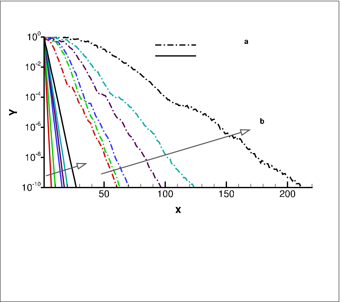
Multigrid preconditioners are effective for this problem, even for high-order bases, and allow the sparse matrix problem to be solved to any level of accuracy. As an example, consider the case of a high-order finite element discretization of the Poisson problem with Dirichlet boundary conditions. Figure 7 shows the convergence history of a multigrid preconditioned conjugate gradient method for basis functions of order through . An algebraic multigrid preconditioner, based on smoothed aggregation using a more general strength measure [22] and optimal interpolation operator [21], is used. We observe only a weak dependence on . Moreover, more advanced multigrid techniques have shown still better scalings for both Poisson and other elliptic problems such as for Stokes flow [15, 20]. Importantly for our principal objective, multigrid preconditioners are well-known to exhibit high parallel efficiency [10, 1]. In the following tests, we use AMG through the BoomerAMG package [13].
2.3 Evaluation of the smooth potential at charge locations
The next step is to evaluate at the charge locations. For standard P3M and PME implementations, this involves interpolation with the Lagrangian or B-spline basis functions from the charge assignment. In contrast, our method requires no interpolation, though interpolation can be used to speed up calculations, if desired. Since the smooth potential exists in each element as a linear combination of coefficients — i.e., the values of at for all points in an element — and the basis functions , the smooth potential is expressed exactly at any point as
| (23) |
where is the number of collocation points in an element. Direct evaluation at the charge locations is straightforward.
2.4 Short-range potential
Our formulation for the exact mesh solution yields a more complex short-range interaction than PME. In addition to , the short-range interaction now also depends on the position of the charge relative to the underlying mesh. Consequently, additional effort is required to evaluate the short-range interaction. However, the calculation is local, so it does not inhibit parallel efficiency.
The short-range potential at point due to a charge located at is
| (24) |
where
| (25) |
Though feasible, performing accurate quadrature for each screen individually is computationally expensive. We therefore shift a significant portion of this computational effort to a pre-processing step, for which there are multiple options.
One approach is to consider a look-up table of pre-computed values for the screen potential evaluated at due to a charge at . These values are represented in a six-dimensional look-up table as , since they are a function of the difference between the evaluation point and the charge location, and also the offset of the charge within its element (which determines the screen).
With some additional computation, but still without resorting to direct evaluation of (25), it is possible to remove the charge offset interpolation to reduce errors. We accomplish this by recognizing the screen’s formulation as a linear combination of basis functions,
| (26) | ||||
| (27) |
This approach yields look-up tables for basis-function potential values . However, for the polynomial nature of the screen leads to non-monotonic decay for some directions within the region where the screen is active, as shown in Figure 5. Consequently, a direct implementation of a look-up table for such functions requires sufficient resolution, which is harder to achieve for larger . For good performance, knowledge of the underlying structure of the screen potentials should be used to inform both the storage locations for the look-up table values and the interpolation method.
2.5 A note about the self term
If the point is the location of a charge, we do not wish to include the potential due to this charge in our calculation. However, we do still need to subtract the screen potential from the charge’s own screen, which is sometimes called the “self” term. We can allow for this by amending our short-range potential expression to include both cases:
| (28) |
2.6 Alternate boundary conditions
The formulation above is presented under the assumption of periodic boundary conditions, which is the simplest case and important for a range of applications. It is straightforward to generalize boundary conditions via the mesh potential . This is accomplished by adjusting for short-range effects present at the boundary and then proceeding in the usual manner for a finite element problem with the given type of boundary conditions. For example, for a Dirichlet boundary condition of on , the condition for our mesh problem becomes
| (29) |
which leads to
| (30) |
A similar approach is used in [14]. This also extends to the case of Neumann or mixed-type boundary conditions, with the usual constraint to address the non-uniqueness of the fully Neumann problem. Free-space conditions impose the usual challenges but are no more difficult for the proposed scheme than for any mesh-based Poisson solver.
3 Performance model
The computational cost of the method for charges is formulated as , where is the total number of degrees of freedom in the mesh. Example CPU time scalings for the major -related components is illustrated in Figure 8(a), with the -dependent mesh solve times shown in Figure 8(b). Given and and assuming on average neighboring elements in the short-range interaction list for each charge, then it is possible to express the coefficients in the linear operation count in terms of . Such a formulation provides a more detailed description of the actual costs of each component of the method and their relationships to the order of the screens.


3.1 Breakdown of costs
Screens of order are built out of basis functions — recall that . The corresponding finite element solve associated with these screens involves degrees of freedom per element and a total of degrees of freedom. We also define the average number of charges per element as .
3.1.1 Screen construction
For each evaluation, the element containing each charge is identified, and the offsets from the center of these elements determined. This incurs a small cost, which we designate . The screen coefficients are then calculated. As shown in (22), assuming pre-computed inverses, this amounts to three matrix-vector multiplications of size , for a cost of . We then multiply the one-dimensional weights, resulting in two additional floating point multiplications. The total cost for determining the screen coefficients is thus
| (screen construction) |
3.1.2 Short-range potential
The cost of evaluating the short-range potential depends on the method chosen for calculating , as discussed in Section 2.4. In addition, there is a cost of due to the singular part of the short-range calculations, which we denote . For a general six-dimensional look-up table, the cost of calculating at a point due to all charges in the short-range interaction volume is , where depends on the order of interpolation used. If three-dimensional look-up tables are used, as we have done in the example calculations of Section 4, then the interpolation is repeated for tables and combined by an inner product with the screen coefficients and a multiplication by for a total of . The cost for the short-range calculation is then
Since , this expression is also written in terms of . However, we assume that in practice, is chosen to be small enough to render this effectively as . Furthermore, if is , this cost is reduced further by calculating the effects of all charges in an element at once in an “element-to-point” operation. To do this, we compile a combined list of for all the charges in any given element, so that the screen potential for this sum at a point as calculated by (27) is the same as if the charges were handled individually. The cost then is then reduced by a factor of yielding
3.1.3 Mesh solve
The “transfer” of the order- screens to a representation in order basis functions by (12) to construct the source in the right-hand side of the finite element solve (5) requires an inner product between a vector containing the screen coefficients with the evaluation of the order- basis functions at the collocation points, followed by a multiplication by . This is done at each degree of freedom within an active screen area, for a total of operations. The multigrid solve for the finite element problem is , with a coefficient that depends on the convergence of the iterations, but is considered low in practice. Overall the mesh solve thus has complexity
3.1.4 Evaluation
The smooth potential is written as a combination of basis functions at the location of each charge, as in (23). Thus evaluation involves basis functions at a cost of operations for each function. However, empirically we find that this cost is minimal in terms of CPU time.
3.2 Summary
The screen creation (mostly due to the “transfer” portion) and short-range interaction calculations are the most costly even for modest values of given the scaling shown above. The relative costs of these two portions of the algorithm depend on choices in short-range calculation method, mesh size, and . For any given cutoff error, decreasing mesh spacing decreases the number of short-range interactions, but results in an increased number of collocation points in the mesh solve. Likewise, increasing also decreases the number of short-range interactions, but at the price of the increased cost of constructing and manipulating screens for larger . Calculating the short-range effects of each individual charge becomes more costly with increased , though at a slower rate than the transfer. The scaling of these components is shown in Figure 9 for cases of to randomly distributed particles in a triply-periodic box with elements. It is noted that once , the singular short-range calculation loses its linearity in . However, the screen potential portion of the short-range calculation retains its linearity due utilization of the “element-to-point” evaluation method.


4 Example calculation
We consider cases with ranging from to unit charges placed in a triply-periodic unit cube of elements with . The exact positions are selected randomly, but distributed so that any given charge experiences both long-range interactions, on the scale of the overall periodic domain size, and short-range interactions of comparable magnitude. This is done to provide a balanced test of both the short-range and smooth portions of our decomposition. To achieve this, the charges are randomly distributed within two smaller cubes: is biased toward positive charges, to , and is biased equally strongly toward negative charges. This set-up is visualized in Figure 10a for .
The potential is then calculated using a short-range interaction of elements (corresponding to a minimum possible value of for the cutoff distance ) for linear through quartic screens. This short-range cutoff is chosen to ensure that the short-range potential of every charge near the cutoff exhibits asymptotic behavior. The short-range calculation uses the approach of (27), with look-up tables. These experiments are tested using a dual, quad-core Intel Xeon E5506 CPU with 48 GB of main memory.
Remark 1.
In our current implementation, we use a variation (but equivalent form) to this construction, in which the values stored in the tables are for “basis screens” instead of screen basis functions. These basis screens, , are the polynomial screens associated with each node in an order- finite element. The values of each table are computed as a Dirichlet finite element solution for Poisson’s equation, with . The computation is completed in a domain larger than the size that will be kept in the look-up table to minimize boundary effects. Because these basis screens follow our moment-canceling rules, they have long-range decay , and the boundary conditions are accurately set by the first terms of the multipole expansion (8). The finite element solver uses basis functions of order , and the look-up tables are stored in terms of their order- basis functions, allowing them to be evaluated and combined in the same way as for all charge locations. We note that because the number of tables and coefficients is unchanged, the computational complexity for the short-range calculation is not altered by this variation.
Upon calculation the potential is compared, allowing for a constant which is included in a potential and in this case is equal to the average value of throughout the computational domain, with that of an Ewald summation with large enough resolution that we consider it the “exact” solution. This uses two periodic images in physical space with and four modes for each direction in the Fourier sum. As we see for a representative calculation in Figure 11, the method has super-algebraic convergence with .


In each of these tests, we use an algebraic multigrid preconditioned GMRES solver with single precision residual tolerance — i.e., . Boomeramg [13] is used and the resulting method yields 8 or fewer iterations in each of the tests reported above. The timing dependence on mesh size is reported in Figure 8(b) where we see that the solver exhibits scaling.
4.1 Estimated memory requirements
The memory requirements of the method in our example calculations are classified as finite element matrices or particle-related arrays. As the number of elements increases, the finite element matrices comprise a majority of the total allocated memory, as demonstrated in the following for the case of :
| Order of | Particle | FE matrices | FE matrices |
|---|---|---|---|
| screens | arrays | () | () |
| linear (): | 184 MB | 39 MB ( 18%) | 844 MB ( 81%) |
| quartic (): | 1120 MB | 1290 MB ( 52%) | 27 600 MB ( 95%) |
As the polynomial order increases — e.g. , which corresponds with a th order basis for the finite element solve — this effect increases as expected. We note that this memory footprint is typical for high-order FEM, but more optimal methods do exist [18].
5 Discussion
5.1 Comparison to PME
While the method proposed here incorporates several advantageous features of PME, there are several notable differences that may offer benefits in certain settings. Our method no longer relies on the FFT, which may be limiting a extreme scales (in comparison to other Poisson solvers) and forces an assumption of structure on the compute geometry. The key is the introduction of a mesh-based screen, which introduces additional complexities locally, but also allows for a more general decomposition of the problem. There are particle-mesh variants that use finite elements — e.g., some PIC methods [6, 23] — but these have been proposed with a symmetric screen, which must be resolved on the mesh. We avoid this approximation, but at the cost of more intricate screen functions, which are constructed with (and the resulting potentials evaluated by) using memory-local operations. This fundamental difference hampers direct cost comparison with PME/P3M methods, which perform well when global FFTs do not impose restrictions. Still, we make some general comparisons in the following.
The locality of the new method comes at the cost of more intricate screens, which incur an cost when represented by -order basis functions as discussed in Section 3. This is larger than the cost of the -order B-spline interpolations in PME. However, the polynomial order in the present scheme and the B-spline order in PME are only loosely related. The B-spline order affects the overall accuracy of the PME method since it affects the resolution of the mesh description of the smooth potential. The polynomial order in the present method does not, since the mesh solve is exact for any . Instead, affects via the decay of the screened potential as shown in Figure 6. This is important, since for uniform charge density the cost of point-to-point interactions scales with volume . An independent Ewald splitting parameter sets the corresponding truncation error at fixed cut-off radius for PME.
Similarly, the mesh density has different implications in the two methods. As with the B-spline order, the mesh density in PME affects the accuracy by providing more resolution for the potential. A denser mesh does not affect the short-range calculation, but requires more global communication for the FFT. In contrast, the mesh density in the present scheme decreases the communication burden for the short-range component of the calculation by reducing the number of interactions included for a given , since the cut-off radius is scaled by the mesh size, unlike in PME. The communication required of the mesh solver is that of multigrid.
5.2 Comparison to FMM
The method presented in this paper shares several attractive features of the fast multipole method, most notably the linear scaling. The relative merits in comparison to FMM are likely application dependent, and the preferred choice depends on several factors. Though intricate, the low communication burden of FMM leads to efficient implementations [19]. Both methods become expensive with increased , the basis order in the present scheme or the multipole expansion order for FMM. Yet the highly local work load of the proposed high-order screens is more suitable for emerging architectures with accelerators. Unlike FMM, the present method is not naturally adaptive to larger regions without singularities — e.g., charges. The degree to which FMM takes advantage of this in parallel depends on load balancing issues of the system.
5.3 Other considerations
For dynamic application, the conservation properties of the overall scheme are important, such as conservation of energy in molecular dynamics simulations. Since we are only evaluating potentials in this paper, we do not consider momentum or energy conservation in detail. For the formulation as presented, the operators we demonstrate do not exactly satisfy the symmetry discussed by Hockney and Eastwood [16], so exact momentum conservation is not anticipated. Moreover, as the basis functions are not differentiable at the collocation points, straightforward analytical differentiation of the potentials is not always possible.
The nature of the mesh solve in the presented method lends itself to varied boundary conditions since the fundamental formulation of the algorithm does not change when the boundary conditions are changed. As with PME, periodic boundary conditions are the simplest to implement in our method, and require no extra effort beyond creating a finite element matrix that honors the periodic structure of the mesh. As presented in Section 2.6, Dirichlet and Neumann boundary conditions simply require calculations to allow for any short-range effects already present on the surface before applying the conditions to the finite element problem.
The method is also extensible to non-uniform meshes common in finite element discretizations without fundamental changes. The main differences for general meshes is in the cost of the method. The screens are still built in the same way, that is, they still solve (13). However, the discussed simplifications of the screen coefficient calculations depend on a regular, rectangular mesh and are not applicable to an unstructured mesh with general quadrilateral elements. Thus, the flexibility of a complex mesh is balanced with the benefits of localizing the mesh cells. Likewise, the short-range potential becomes more difficult to generalize due to the many different shapes a screen could take based on the shapes of the elements composing it. Gaining accurate values for the short-range potentials may require quadrature-based evaluations for each pair of interacting charges. However, the locality and structured character of these operations is expected to coincide with high-throughput accelerators.
In our demonstration, we have presented one choice for the support of the screens. Another possible variation of the method is to limit the screens to have support in only the element containing the charge, so that each screen includes only degrees of freedom interior to the element and not those on the faces. Using the same multipole representation to construct the screen, this choice results in a loss of two powers in the short-range decay of the screens — e.g., for the screen yields a far-field decay instead of , while of course still requiring in the mesh solve (and all the cost incurred by this order of ). However, the more compact screen provides an asymptotic decay rate starting at instead of (see Figure 6), which reduces the cost through reducing for certain target accuracies. The local composition of these one-element screens also facilitates the move to unstructured meshes, helping alleviate some of the additional cost in the screen-related calculations.
In constructing our screens, we have chosen to maximize the far-field decay rate. Some simulation goals may be better served by other choices — e.g., by a weighted objective function. In such cases, a least-squares optimization might provide screens with advantageous properties to meet overall simulation objectives. We have also restricted our discussion to purely polynomial basis functions. Given the regularity of the underlying Green’s function, basis enrichments with specially designed functions chosen to increase the short-range decay likely enhance the overall performance of the method, though this also disrupts the exactness of the mesh solve.
Acknowledgments
This work was supported by the Computational Science & Engineering program at the University of Illinois at Urbana-Champaign, NSF 09–32607 and 13–36972, NSF DMS 07–46676. This material is also based in part upon work supported by the Department of Energy, National Nuclear Security Administration, under Award Number DE-NA0002374. We would also like to thank Doug Fein and the team at the National Center for Supercomputing Applications (NCSA) for their computing resources.
References
- [1] Allison H. Baker, Robert D. Falgout, Tzanio V. Kolev, and Ulrike Meier Yang, Scaling hypre’s multigrid solvers to 100,000 cores, in High-Performance Scientific Computing, Michael W. Berry, Kyle A. Gallivan, Efstratios Gallopoulos, Ananth Grama, Bernard Philippe, Yousef Saad, and Faisal Saied, eds., Springer London, 2012, pp. 261–279.
- [2] D. S. Cerutti and D. A. Case, Multi-level Ewald: A hybrid multigrid/fast Fourier transform approach to the electrostatic particle-mesh problem, J. Chem. Theory Comput., 6 (2010), pp. 443–458.
- [3] David S. Cerutti, Robert E. Duke, Thomas A. Darden, and Terry P. Lybrand, Staggered mesh Ewald: An extension of the smooth Particle-Mesh Ewald method adding great versatility, J. Chem. Theory Comput., 5 (2009), pp. 2322–2338.
- [4] H. Cheng, L. Greengard, and V. Rokhlin, A fast adaptive multipole algorithm in three dimensions, J. Comp. Phys., 55 (1999), pp. 468Ж498.
- [5] Tom Darden, Darrin York, and Lee Pedersen, Particle mesh Ewald: An method for Ewald sums in large systems, J. Chem. Phys., 98 (1993), pp. 10089–10092.
- [6] James W. Eastwood, Particle simulation methods in plasma physics, Comput Phys Commun, 43 (1986), p. 89Ñ106.
- [7] Ulrich Essmann, Lalith Perera, Max L. Berkowitz, Tom Darden, and Hsing Lee et al., A smooth particle mesh Ewald method, J. Chem. Phys., 103 (1995), pp. 8577–8593.
- [8] P. Ewald, Die berechnung optischer und elektrostatischer gitterpotentiale, Ann. Phys., 369 (1921), pp. 253–287.
- [9] Jonathan B. Freund, Electro-osmosis in a nanometer-scale channel studied by atomistic simulation, J Chem Phys, 116 (2002), pp. 2194–2200.
- [10] Hormozd Gahvari and William Gropp, An introductory exascale feasibility study for ffts and multigrid, Parallel and Distributed Processing Symposium, International, 0 (2010), pp. 1–9.
- [11] L. Greengard and V. Rokhlin, A fast algorithm for particle simulations, J. Comp. Phys., 135 (1987), pp. 280–292.
- [12] Leslie Greengard and Vladimir Rokhlin, A new version of the fast multipole method for the Laplace equation in three dimensions, Acta Numerica, 6 (1997), pp. 229–269.
- [13] Van Emden Henson and Ulrike Meier Yang, Boomeramg: a parallel algebraic multigrid solver and preconditioner, Applied Numerical Mathematics, 41 (2000), pp. 155–177.
- [14] Juan P. Hernandez-Ortiz, Juan J. de Pablo, and Michael D. Graham, Fast computation of many-particle hydrodynamic and electrostatic interactions in a confined geometry, Phys. Rev. Let., 98 (2007), p. 140602.
- [15] J. J. Heys, T. A. Manteuffel, S. F. McCormick, and L. N. Olson, Algebraic multigrid for higher-order finite elements, J. Comput. Phys., 204 (2005), pp. 520–532.
- [16] R. W. Hockney and J. W. Eastwood, Computer simulation using particles, Institute of physics publishing, Bristol, 1988.
- [17] J. A. Izaguirre, S. S. Hampton, and T. Matthey, Parallel multigrid summation for the N–body problem, J. Parallel Distrib. Comput., 65 (2005), pp. 949–962.
- [18] RobertC. Kirby, Fast simplicial finite element algorithms using bernstein polynomials, Numerische Mathematik, 117 (2011), pp. 631–652.
- [19] Ilya Lashuk, Aparna Chandramowlishwaran, Harper Langston, Tuan-Anh Nguyen, Rahul Sampath, Aashay Shringarpure, Richard Vuduc, Lexing Ying, Denis Zorin, and George Biros, A massively parallel adaptive fast multipole method on heterogeneous architectures, Commun ACM, 55 (2012), pp. 101–109.
- [20] Luke Olson, Algebraic multigrid preconditioning of high-order spectral elements for elliptic problems on a simplicial mesh, SIAM J. Sci. Comput., 29 (2007), pp. 2189–2209.
- [21] Luke N. Olson, Jacob Schroder, and Raymond S. Tuminaro, A new perspective on strength measures in algebraic multigrid, Numerical Linear Algebra with Applications, 17 (2010), pp. 713–733.
- [22] Luke N. Olson, Jacob B. Schroder, and Raymond S. Tuminaro, A general interpolation strategy for algebraic multigrid using energy minimization, SIAM Journal on Scientific Computing, 33 (2011), pp. 966–991.
- [23] A. C. J. Paes, N. M. Abe, V. A. Serrão, and A. Passaro, Simulations of plasmas with electrostatic PIC models using the finite element method, Braz J Phys, 33 (2003), pp. 411–417.
- [24] E.L. Pollock and Jim Glosli, Comments on p3m, fmm, and the ewald method for large periodic coulombic systems, Comput Phys Commun, 95 (1996), pp. 93–110.
- [25] C. Sagui and T. Darden, Multigrid methods for classical molecular dynamics simulations of biomolecules, J. Chem. Phys., 114 (2001), pp. 6578–6591.
- [26] Bilha Sandak, Multiscale fast summation of long-range charge and dipolar interactions, J. Comput. Chem., 22 (2001), pp. 717–731.
- [27] R. D. Skeel, I. Tezcan, and D. J. Hardy, Multiple grid methods for classical molecular dynamics, J Comput Chem., 23 (2002), pp. 673–684.
- [28] Anna-Karin Tornberg and Leslie Greengard, A fast multipole method for the three-dimensional Stokes equations, J. Comp. Phys., 227 (2008), pp. 1613Ж1619.
- [29] S.K. Veerapaneni, A. Rahimian, G. Biros, and D. Zorin, A fast algorithm for simulating vesicle flows in three dimensions, J. Comp. Phys., 230 (2011), pp. 5610–5634.
- [30] Haitao Wang, Ting Lei, Jin Li, Jingfang Huang, and Zhenhan Yao, A parallel fast multipole accelerated integral equation scheme for 3D Stokes equations, Int. J. Numer. Meth. Engng, 70 (2007), pp. 812–Ð839.