Nontrivial paths and periodic orbits of the $T$-fractal billiard table.Thanks: The work of M. L. Lapidus was partially supported by the National Science Foundation under the research grants DMS-0707524 and DMS-1107750, as well as by the Institut des Hautes Etudes Scientifiques (IHES) in Bures-sur-Yvette, France, where he was a visiting professor while part of this paper was written. The work of R. G. Niemeyer was partially supported by the National Science Foundation under the MCTP grant DMS-1148801, while a postdoctoral fellow at the University of New Mexico, Albuquerque.

A fractal billiard table is a planar billiard table $\Omega(F)$ where the boundary $\partial\Omega(F)=F$ is a fractal curve. In this paper, we take $\Omega(F)$ to be the $T$-fractal billiard table shown in Figure 1. In [CheNie1], the fractal billiard table is a self-similar Sierpinski carpet billiard table. In [LapNie1, LapNie2, LapNie3], the fractal billiard table under consideration was the Koch snowflake fractal billiard table. In [LapNie4], recent results on the Koch snowflake fractal billiard table and a self-similar Sierpinski fractal billiard table are surveyed and the $T$-fractal billiard table is introduced; preliminary results regarding the $T$-fractal billiard table were presented without proof. The $T$-fractal is not, strictly speaking, a self-similar set nor is it the finite union of self-similar sets. However, as we demonstrate at the end of this introduction, $\Omega(\mathscr{T})$ can be constructed by way of a particular iterated function system whose contraction mapping is denoted by $\Phi$. We illustrate in Figure 1 how to construct the $T$-fractal billiard.

We mention that the $T$-fractal is not the unique fixed point attractor of $\Phi$, this being a technical detail that does not take away from the fractality of the set. Rather, the unique fixed point attractor of $\Phi$ is of great interest and is hereafter referred to as the set of elusive points of the fractal billiard table; such points are those that are never found in any finite approximation and a formal definition of elusive point is given in Definition 2.2, with further elaboration given in Remark 2.3. The geometry of $\Omega(\mathscr{T})$ will aide us in our analysis of nontrivial paths (in the sense of Definition 2.12) and periodic orbits of the $T$-fractal billiard table.

The $T$-fractal enjoys particular properties not found in the Koch snowflake and a self-similar Sierpinski carpet. Indeed, the Koch snowflake $K\!S$ is a nowhere differentiable curve bounding a region with finite area. Furthermore, a self-similar Sierpinski carpet contains no area. By contrast, the T-fractal bounds a region with finite area, yet a nontrivial portion of the boundary remains differentiable. Hence, determining directions for which one gets periodic orbits is a much easier task compared to finding such orbits in the Koch snowflake fractal billiard table. Additionally, the set of directions for which one finds periodic orbits of the $T$-fractal billiard table is countably infinite, this being in contrast to a self-similar Sierpinski carpet billiard table, where the number of directions for which periodic orbits occur is finite (this finite value depending exclusively on the scaling ratio of the carpet). We note that Propositions 3.1 and 3.2 below first appeared without proof and were stated under more restrictive conditions in [LapNie4]; in this paper, we provide detailed proofs of these more general propositions, among many other results.

The overarching themes of the research program on fractal billiards and fractal flat surfaces are topological and measure-theoretic in nature. In one instance, we seek to understand what constitutes a periodic orbit of a fractal billiard table. In another instance, we seek to understand when an orbit may be dense in a fractal billiard table. More generally, we eventually seek to answer the question asking which directions yield flows that are closed and which yield flows that are ergodic (i.e., where almost every orbit is uniformly distributed in the fractal billiard table).

Of course, all of this relies on the existence of a well-defined billiard map and phase space. Defining such a map and space for a fractal billiard table is a very difficult task, one that the authors have yet to accomplish. In order to work towards the abovementioned goals in the absence of a billiard map and phase space, we rely on the geometric properties of the fractal to construct what we are calling nontrivial paths of a fractal billiard table. We are ultimately interested in nontrivial paths reaching elusive points¹¹ 1 An elusive point is never a point of any finite approximation and is formally defined in Definition 2.2. of a fractal billiard table. In the case of the $T$-fractal billiard (and, likewise, the Koch snowflake fractal billiard table), any pointmass on a trajectory that results in the pointmass reaching an elusive point does so in an increasingly confined manner. It is then natural to ask how a pointmass will “reflect” off from an elusive point and under what conditions will such an orbit

1. (1)

   form a periodic orbit of the fractal billiard table (i.e., return to the elusive point infinitely often in the same direction),

2. (2)

   terminate at an elusive point, because of some sort of inherent ambiguity,

3. (3)

   or manage to fill all or part of some nontrivial 2-dimensional subset of $\Omega(\mathscr{T})$ (either uniformly or not).

We answer in part these questions by giving a variety of sufficient conditions under which 1) a periodic orbit of $\Omega(\mathscr{T})$ exists and, more generally, 2) a nontrivial path²² 2 A path that manages to never be confined to any finite approximation of $\Omega(\mathscr{T})$. of $\Omega(\mathscr{T})$ exists; see Definition 2.12. In the case of the $T$-fractal billiard (and, also, the Koch snowflake fractal billiard), there are trajectories yielding orbits that reach elusive points. The geometric properties of the $T$-fractal billiard lend themselves well to the description of such trajectories, this being the major focus of §3 and §4.

The paper is organized as follows. In §2, the necessary background is given so that a reader not familiar with mathematical billiards or the terminology developed in earlier works may be able to understand the remainder of the paper. Sufficient conditions for sequences of compatible periodic orbits are given in §3. In §4, we build upon the concepts developed in §3 and show (via an explicit construction) that there exist nontrivial paths and periodic orbits in the $T$-fractal billiard $\Omega(\mathscr{T})$. Then, in §5, we introduce an important example of a nontrivial path with an initial direction that is irrational, yet reaches an elusive point of the $T$-fractal billiard in a way that is similar to how particular nontrivial paths with rational initial directions reach their respective elusive points. This is an unintuitive behavior that begins to depart from the classical theory of billiards on square tiled billiard tables. Finally, in §6, we discuss some of our results and propose directions for future research.

As we previously mentioned, the set of elusive points, which we denote by $\mathscr{E}$, is the unique fixed point attractor of $\Phi$. Since $\Phi([-1,2]\times\{3\})=[-1,2]\times\{3\}$ and the attractor of $\Phi$ is unique, we see that $\mathscr{E}=[-1,2]\times\{3\}$.

For the reader’s easy reference, we provide in this section various definitions appearing in previous joint works; see [CheNie1, LapNie1, LapNie2, LapNie3, LapNie4]. However, the notation in all of the definitions will reflect the fact that we are discussing the $T$-fractal billiard table, which will significantly simplify the exposition. Particular definitions (e.g., the definitions for compatible initial conditions and a sequence of compatible initial conditions) will be phrased in full generality so that the reader may be able to understand the results appearing in the abovementioned works.

In order to understand the following notations and definitions, we first discuss the phase space for the billiard dynamics on a polygonal billiard table. If $\Omega(B)$ is a polygonal billiard with boundary $B$, then we consider the Cartesian product $\Omega(B)\times S^{1}$, where $S^{1}$ is the unit circle in $\mathbb{R}^{2}$. As a subset of the tangent bundle on $\mathbb{R}^{2}$, the flow on $\Omega(B)\times S^{1}$ is only partially defined, since any trajectory on $\Omega(B)$ would intersect with $B$. For points of $\Omega(B)$ that are not vertices, one can define an equivalence relation $\sim$ on $\Omega(B)\times S^{1}$ that identifies outward pointing vectors with inward pointing vectors so that the flow on $\Omega(B)\times S^{1}$ can be continued in a continuous manner at the boundary. That is, if $\rho_{i}$ is the reflection through the edge $e_{i}$ of $B$, then for a point $x$ on $e_{i}$ which is not a vertex of $B$, we write that $(x,\theta)\sim(x,\rho_{i}(\theta))$; for points in the interior of $\Omega(B)$, $(x,\theta)$ is equivalent to itself and to no other ordered pair.

However, for points of $B$ that are vertices, a geodesic cannot always be continued in a well-defined manner. A priori, one terminates the geodesic when it intersects a vertex of $B$. More precisely, if $x$ is a vertex of $B$, then $(x,\theta)\sim(x,\rho(\theta))$ for every $\rho$ in the group generated by $\rho_{i}$ and $\rho_{j}$, the reflections through the edges $e_{i}$ and $e_{j}$, respectively. As one may then see, in certain situations, one can show that a geodesic intersecting a vertex of $B$ can be continued in a well-defined manner. This occurs when there is only one $\rho^{\prime}$ in the group generated by the elements $\rho_{i}$ and $\rho_{j}$ such that $\rho^{\prime}(\theta)$ is an inward pointing direction at the vertex $x$. Thus, one can define the quotient space $(\Omega(B)\times S^{1})/\!\sim$ to be the tangent bundle of $\Omega(B)$.

In the context of a prefractal approximation $\Omega(\mathscr{T}_{n})$ of the $T$-fractal billiard, this is when a billiard orbit intersects a right angle of $\Omega(\mathscr{T}_{n})$ (when one measures the angle from the interior of $\Omega(\mathscr{T}_{n})$). When a billiard orbit intersects a vertex with an obtuse angle (still when measured from the interior of $\Omega(\mathscr{T}_{n})$), one cannot determine the continuation of the geodesic in a well-defined manner. Hence, the geodesic terminates.

In general, one restricts one’s attention to $(B\times S^{1})/\!\sim$. When defined, the map $f_{B}\!:(B\times S^{1})/\!\sim\,\,\rightarrow(B\times S^{1})/\!\sim$ is a map on the set of equivalence classes. The representative element of an equivalence class $[(x,\theta)]$ is the element $(x,\theta)$, where $\theta$ is the inward pointing direction based at $x$. As such, one simplifies notation slightly by considering $f_{B}$ (again, when defined) as a map on the representative elements; i.e., $f_{B}(x,\theta)=(x^{\prime},\rho_{i}(\theta^{\prime}))$, where $\rho_{i}(\theta^{\prime})$ is the reflection of the angle $\theta^{\prime}$ through the side $e_{i}$ containing $x^{\prime}$. The map $f_{B}$ is called the billiard map (of $\Omega(B)$).

Being an interval in the plane, the set $\mathscr{E}$, though stretched, is a copy of the unit interval $[0,1]$. As a result, an elusive point can be given an address in terms of $L$’s and $R$’s. Geometrically, this is motivated by the fact that with each iteration of $\Omega(\mathscr{T}_{n})$, one adds to each scaled copy of $\Omega(\mathscr{T}_{0})$ two smaller copies of $\Omega(\mathscr{T}_{0})$ of scale $2^{-n-1}$, a left copy and a right copy; see Figure 4. We want to distinguish between what we call rational and irrational elusive points. Let $x\in\mathscr{E}$. Then $x$ is called a rational elusive point if the address for $x$ is a preperiodic sequence of $L$’s and $R$’s. Otherwise, $x$ is called an irrational elusive point; see Figure 4.

In this article, $x_{n}^{0}$ will never be on a segment of $\mathscr{T}_{n}$ to be removed in the construction of $\Omega(\mathscr{T}_{n+1})$. Hence, there exists a nonnegative integer $i$ such that $x_{n}^{0}=x_{i}^{0}$ for all $n\geq i$ as a point in the plane.⁶⁶ 6 We note that for $m\neq n$, $x_{n}^{0}$ and $x_{m}^{0}$ really lie in two different spaces. When we say that they are equal, we are actually implying that some embeddings of $x_{n}^{0}$ and $x_{m}^{0}$ into the plane are equal. This is a technical detail that will not cause any problems, but is worth mentioning. See Figure 8 for an example of a sequence of compatible orbits.

As was alluded to at the beginning of this section, Definitions 2.4 and 2.6 were stated in full generality so that the reader may understand the results in the aforementioned articles, should they refer back to them for examples of periodic orbits and nontrivial paths of other fractal billiard tables (namely, the Koch snowflake fractal billiard and a self-similar Sierpinski carpet fractal billiard table studied, respectively, in [LapNie1–5], [CheNie1], [LapNie4]). As we see in Figure 5, it may be that two initial conditions are compatible and $x^{0}_{0}=x^{0}_{n}$ for all $n\geq 0$. Also, it is possible, as shown in Figure 6, that $x_{n}^{0}\neq x_{n+1}^{0}$ for, in this case, $n=1$, thereby necessitating a more general definition.⁷⁷ 7 As we mentioned, however, we will always assume that $x_{i}^{0}$ is not on a segment to be removed in the construction of $\Omega(\mathscr{T}_{i+1})$ from $\Omega(\mathscr{T}_{i})$. In the case of the Koch snowflake, we give an example in Figure 7 that demonstrates the necessity for the full generality of Definitions 2.4 and 2.6.

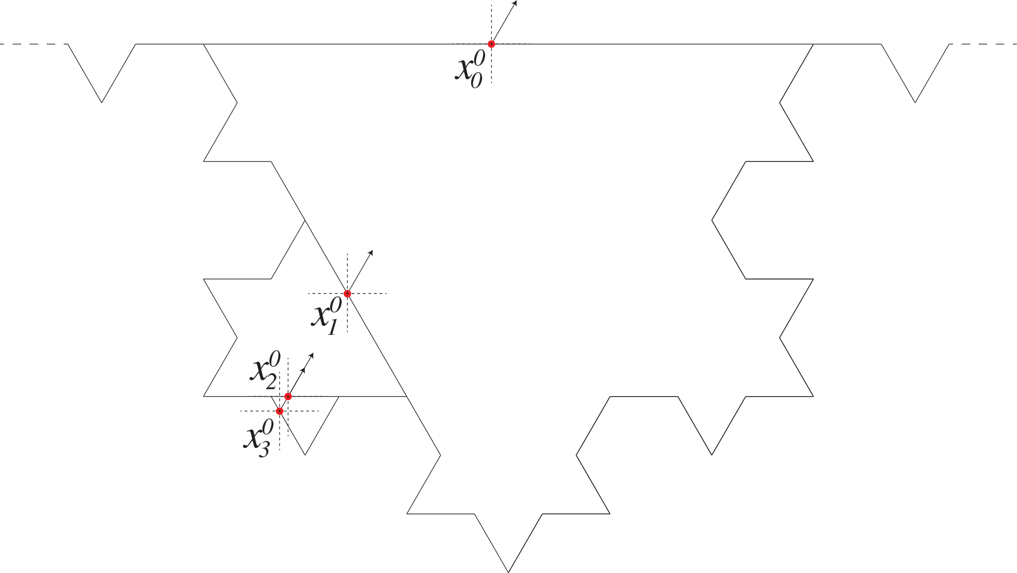
If $\mathscr{O}_{m}(x_{m}^{0},\theta_{m}^{0})$ is an orbit of $\Omega(\mathscr{T}_{m})$, then $\mathscr{O}_{m}(x_{m}^{0},\theta_{m}^{0})$ is a member of a sequence of compatible orbits $\{\mathscr{O}_{n}(x_{n}^{0},\theta^{0})\}_{n=i}^{\infty}$, for some $i\leq m$. It is clear from the definition of a sequence of compatible orbits that such a sequence is uniquely determined by the first orbit $\mathscr{O}_{i}(x_{i}^{0},\theta^{0})$. Since the initial condition of an orbit determines the orbit, we can say without any ambiguity that a sequence of compatible orbits is determined by an initial condition $(x_{i}^{0},\theta^{0})$. Consequently, one is then in a position to discuss particular types of sequences of compatible orbits, namely, sequences where, for a given sequence, every orbit in that sequence has the same property. More precisely, let $\mathcal{P}$ be a property (resp., $\mathcal{P}_{1},...,\mathcal{P}_{j}$ a list of properties). If every orbit in a sequence of compatible orbits has the property $\mathcal{P}$ (resp., a list of properties $\mathcal{P}_{1},...,\mathcal{P}_{j}$), then we call such a sequence a sequence of compatible $\mathcal{P}$ (resp., $\mathcal{P}_{1},...,\mathcal{P}_{j}$) orbits.

In general, for any $j\geq 1$, we let $\upsilon_{n}^{j}$ be the $j$th return time of the orbit $\mathscr{O}_{n}(x_{n}^{0},\theta_{n}^{0})$. As previously mentioned, given a sequence of compatible orbits $\{\mathscr{O}_{n}(x_{n}^{0},\theta^{0})\}_{n=i}^{\infty}$, the geometry of the $T$-fractal dictates that there exists $m\geq i$ such that $x_{n}^{0}=x_{m}^{0}$ for every $m\geq n$. This implies that there exists $m\geq i$ such that for every $j\geq 1$, $x_{n}^{\upsilon^{j}_{n}}$ is on the same segment as $x_{m}^{0}$ for all $n\geq m$.

Let $\{\mathscr{O}_{n}(x_{n}^{0},\theta^{0})\}_{n=i}^{\infty}$ be a sequence of compatible orbits such that $\tau_{n}<\infty$ for every $n\geq i$. From now on, we denote by $\mathscr{N}_{n}(x_{n}^{0},\theta^{0})$ the path given by $\mathscr{O}_{n}(x_{n}^{0},\theta^{0})_{\tau_{n}}$. We next define what it means for a path in $\Omega(\mathscr{T})$ to be a nontrivial path. (Recall that, intuitively, a nontrivial path in $\Omega(\mathscr{T})$ is one that manages to never remain confined in any finite approximation $\Omega(\mathscr{T}_{n})$ of the billiard table $\Omega(\mathscr{T})$.)

In Figure 9, the first three paths $\mathscr{N}_{i}(x_{i}^{0},\theta^{0})$, $i=0,1,2$, of a sequence $\{\mathscr{N}_{n}(x_{n}^{0},\theta^{0})\}_{n=0}^{\infty}$ derived from a particular sequence of compatible periodic orbits, are given.

As was mentioned just after Definition 2.8, we denote by $\upsilon_{n}^{j}$ the $j$th return time of the orbit $\mathscr{O}_{n}(x_{n}^{0},\theta_{n}^{0})$. We now define what it means for an orbit of $\Omega(\mathscr{T})$ to be a recurrent orbit of the $T$-fractal billiard table. We also note that Definitions 9–2.16 below are specific to the $T$-fractal billiard. However, it is plausible that one may be able to appropriately generalize them so as to account for what have been called periodic orbits of the given fractal billiard table(s) in each of [CheNie1, LapNie1, LapNie2, LapNie3, LapNie4]. Moreover, in some of the aforementioned works, we have indicated that a periodic orbit of a fractal billiard table may be the suitable limit of a sequence of compatible periodic orbits, namely the Hausdorff--Gromov limit.⁸⁸ 8 We have discussed the use of the Hausdorff–Gromov limit since, technically speaking, each orbit is in an entirely different space, though each may project down onto the plane and into a billiard table that contains the previous prefractal billiard table approximation. In the results presented in the subsequent sections, we will see how the Hausdorff–Gromov limits of particular sequences of compatible orbits do in fact produce orbits of the $T$-fractal billiard satisfying Definition 2.15. Definitions 9–2.16 remain more general in the event that the Hausdorff–Gromov limit of a sequence of compatible periodic orbits cannot be calculated or does not exist. In the latter case, we may still see that such (perhaps, pathological) examples satisfy Definition 2.15, but exhibit some oddity that prevents them from being the Hausdorff–Gromov limit of a sequence of compatible orbits.

Figure 8 gives an illustration of a sequence of points $\{x_{n}^{\upsilon_{n}}\}_{n=0}^{\infty}$ converging to some $x$ in the unit-interval base of $\Omega(\mathscr{T})$. Moreover, we consider $x$ to be the point of first return for the orbit of the fractal billiard table. In general, it does not have to be the case that $x_{n}^{\upsilon_{n}^{j}}=x^{\upsilon^{j}}$ for sufficiently large $n$ and all $j\geq 1$. In fact, in many of the examples and results that we will present, it is the case that $x_{n}^{\upsilon_{n}}\neq x_{m}^{\upsilon_{m}}$, whenever $n\neq m$; see, for example, Figure 8. We now formally define what it means for an orbit to be a periodic orbit of $\Omega(\mathscr{T})$.

The three orbits shown in Figure 8 are part of a sequence of compatible orbits satisfying Definitions 9 and 2.15. As one may be able to deduce from Figure 8, $x_{n}^{\upsilon_{n}}\neq x_{m}^{\upsilon_{m}}$ for all $n\neq m$, but $x_{n}^{\upsilon_{n}}\to x^{\upsilon}$ as $n\to\infty$ where $x^{\upsilon}=x^{0}$ and $x^{0}:=x_{0}^{0}$. The sequence of compatible orbits illustrated in Figure 8 is a sequence of compatible orbits where $\mathscr{O}_{n}(x_{n}^{0},\theta^{0})\neq\mathscr{O}_{m}(x_{m}^{0},\theta^{0})$ for all $n\neq m$. On the other hand, Definitions 9 and 2.15 are phrased in such a way as to also account for what we will see is the trivial limit of an eventually constant sequence of compatible periodic orbits; see Definition 3.5 and Theorem 3.10.

When we speak of a singular orbit of $\Omega(\mathscr{T}_{n})$, we mean that the forward orbit is a singular orbit. This is to differentiate from what are called saddle connections.¹⁰¹⁰ 10 A saddle connection of a polygonal billiard table is an orbit that connects two singularities, or corners, of the billiard table. The reason for this distinction is that an orbit with $\theta^{0}$ such that $\tan\theta^{0}$ is irrational may yield a singular forward orbit, yet starting from the same point $x_{n}^{0}$, but with a new direction of $\pi-\theta^{0}$, will yield a dense orbit, or vice-versa.

In the classical case of a rational billiard table, when a pointmass intersects with a corner where the orbit cannot be continued in a well-defined manner, we terminate the trajectory. It is very ambiguous how a pointmass would continue in such a situation. In Part (1) of Definition 2.16, the fact that, for some $j\geq 1$, the sequence $\{x_{n}^{\upsilon^{j}_{n}}\}_{n=i}^{\infty}$ does not converge to a single limit point highlights an analogous ambiguity for the pointmass in the fractal billiard table. In §5, we give an example of a sequence of compatible orbits satisfying Part (2) of Definition 2.16. While no example of a sequence of compatible orbits satisfying Part (1) has yet been found, this does not mean that such a definition is unnecessary. Indeed, this definition captures the essence of a singular orbit, namely, that such an orbit cannot be continued in a well-defined manner. For each $j\geq 1$, the set $\{x_{n}^{\upsilon_{n}^{j}}\}_{n=i}^{\infty}$ having two or more accumulation points is analogous to an orbit having two or more ways of continuing past a nonremovable singularity (i.e., one for which reflection cannot be well defined). We believe that such an example can be found, this being the focus of [JohNie2].

In this section, we give sufficient conditions for when a sequence of compatible orbits is a sequence of compatible periodic orbits. Our goal here is to lay the foundation for the study of the limiting behavior of particular sequences of compatible periodic orbits considered in §4. In §5, we will give an example of a sequence of compatible singular orbits that yields a nontrivial path of the $T$-fractal billiard table. Such a nontrivial path will constitute a singular orbit of $\Omega(\mathscr{T})$.

We remind the reader that the geometry of $\Omega(\mathscr{T}_{0})$ is given in Figure 2. Determining which intercepts and slopes yield line segments in the plane that avoid lattice points of the form $(\frac{a}{2^{c}},\frac{b}{2^{d}})$, with $c$ and $d$ nonnegative integers, is equivalent to specifying an initial condition of an orbit of a square billiard table that avoids corners of the billiard table. Extending this reasoning to $\Omega(\mathscr{T})$, we can determine various sufficient conditions for the existence of a sequence of compatible periodic orbits of the prefractal billiard tables $\Omega(\mathscr{T}_{n})$, for $n\geq 0$.

Specifically, using the fact that an appropriately scaled square billiard table tiles $\Omega(\mathscr{T}_{n})$, we can reflect-unfold such an orbit in $\Omega(\mathscr{T}_{n})$ in order to determine an orbit of $\Omega(\mathscr{T}_{n})$.

Note that the condition (3) above is automatically satisfied if the slope $m$ is irrational.

Finally, Propositions 3.1 and 3.2 (combined with the fact that an initial condition of an orbit of $\Omega(\mathscr{T}_{i})$, $i\geq 0$, determines a sequence of compatible orbits $\{\mathscr{O}_{n}(x_{n}^{0},\theta^{0})\}_{n=i}^{\infty}$), allow us to determine a countably infinite family of sequences of compatible periodic orbits. We state this as a theorem.

We now introduce a specific family of sequences of compatible periodic orbits. A sequence of compatible periodic orbits in such a family will clearly have a trivial limit, this point being discussed at the end of §4.

It should be made clear that a sequence of compatible dense orbits given by $\{\mathscr{O}_{n}(x_{n}^{0},\theta^{0})\}_{n=i}^{\infty}$ will never be an eventually constant sequence of compatible orbits, because we are concerned with both the forward orbit and the backwards orbit simultaneously, though the notation may belie this fact; this is another subtle difference between an orbit and a nontrivial path. Suppose $\{\mathscr{O}_{n}(x_{n}^{0},\theta^{0})\}_{n=i}^{\infty}$ yields a singular orbit of $\Omega(\mathscr{T})$, in the sense that each (forward) orbit $\mathscr{O}_{n}(x_{n}^{0},\theta^{0})$ is a singular orbit. Instead, now consider the sequence of compatible orbits $\{\mathscr{O}_{n}(x_{n}^{0},\pi-\theta^{0})\}_{n=i}^{\infty}$. Such a sequence of compatible orbits is never eventually constant, since each orbit must be uniformly distributed in its respective billiard table. We will see an example of this phenomenon in §5.

The following two lemmas are necessary for establishing sufficient conditions for the existence of a particular family of eventually constant sequences of compatible periodic orbits of prefractal billiard tables.

As discussed in the caption of Figure 11, Figure 12 illustrates the construction of an eventually constant sequence of compatible periodic orbits. Such a sequence of compatible periodic orbits is guaranteed to exist by Theorem 3.10.

In §3, we showed that there are sequences of compatible periodic orbits that are eventually constant; see Theorem 3.10 and Figure 12. In this section, we will focus on determining nontrivial paths and periodic orbits of the $T$-fractal billiard. Specifically, we will be focusing on determining periodic orbits and nontrivial paths from sequences of compatible orbits with certain initial conditions (recall that a sequence of compatible orbits is determined by the initial condition of the first orbit in the sequence of compatible orbits). Such initial conditions will be of the form $x_{0}^{0}\neq m2^{-l}$, with $m$ and $l$ being positive integers and $\theta^{0}$ such that $\tan\theta^{0}=\pm\frac{1}{p}$, where $p$ is an odd positive integer. Then, the initial condition $(x_{0}^{0},\theta^{0})$ satisfies Theorem 3.3, meaning that $\{\mathscr{O}_{n}(x_{n}^{0},\theta^{0})\}_{n=0}^{\infty}$ is a sequence of compatible periodic orbits. What we will now see is that $\{\mathscr{O}_{n}(x_{n}^{0},\theta^{0})\}_{n=0}^{\infty}$ is not an eventually constant sequence of compatible periodic orbits. More to the point, we will see that for every $n\geq 0$, $\tau_{n}<\infty$, $\tau_{n}<\upsilon_{n}$ and $\mathscr{O}_{n}(x_{n}^{0},\theta^{0})_{\tau_{n}}=\mathscr{N}_{n}(x_{n}^{0},\theta^{0})$ will be part of a nontrivial path of $\Omega(\mathscr{T})$, where such a nontrivial path reaches a rational elusive point if and only if $x_{0}^{0}$ is a rational value. In §5, we provide an example of a sequence of compatible singular orbits that yields a nontrivial path. We begin with a specific example of the former as a motivation for some of the following results.

References

- [AcST] Achdou, Y. Sabot, C., Tchou, N.: Diffusion and propagation problems in some ramified domains with a fractal boundary, M2AN Math. Model. Numer. Anal. No. 4, 40 (2006), 623–652.
- [CheNie1] Chen, J. P., Niemeyer, R. G.: Periodic billiard orbits of self-similar Sierpinski carpets, J. Math. Anal. Appl. 416 (2014), 969–994.
- [GaStVo] Galperin, G., B., Stepin, A. M., Vorobets, Ya.: Periodic billiard trajectories in polygons, Russian Math. Surveys No. 3, 47 (1992), 5–80.
- [Gut1] Gutkin, E.: Billiards on almost integrable polyhedral surfaces, Erg. Th. and Dyn. Syst. 4 (1984), 569–584.
- [GutJu1] Gutkin, E., Judge, C.: The geometry and arithmetic of flat surfaces with applications to polygonal billiards, Math. Res. Lett. 3 (1996), 391–403.
- [GutJu2] Gutkin, E., Judge, C.: Affine mappings of flat surfaces: Geometry and arithmetic, Duke Math. J. 103 (2000), 191–213.
- [Hoo] Hooper, W. P.: The invariant measures of some infinite interval exchange maps, Geometry and Topology 19 (2015), 1895–2038.
- [HuLeTr] Hubert, P., Lelievre, S., Troubetzkoy, S.: The Ehrenfest wind-tree model: periodic directions, recurrence, diffusion, Journal für die Reine und Angewandte Mathematik 656 (2011), 223–244.
- [HuSc] Hubert, P., Schmidt, T.: An introduction to Veech surfaces, in: Handbook of Dynamical Systems, vol. 1B (A. Katok and B. Hasselblatt, eds.), Elsevier, Amsterdam, 2006, pp. 501–526.
- [JohNie1] Johnson, C. C., Niemeyer, R. G.: An interval exchange transformation on a fractal flat surface, in progress, 2016.
- [JohNie2] Johnson, C. C., Niemeyer, R. G.: A computational investigation of a particular nontrivial path, in progress, 2016.
- [LapNie1] Lapidus, M. L., Niemeyer, R. G.: Towards the Koch snowflake fractal billiard—Computer experiments and mathematical conjectures, in: Gems in Experimental Mathematics (T. Amdeberhan, L. A. Medina and V. H. Moll, eds.), Contemporary Mathematics, Amer. Math. Soc., Providence, RI, 517 (2010), pp. 231–263. [E-print: arXiv:math.DS.0912.3948v1, 2009.]
- [LapNie2] Lapidus, M. L., Niemeyer, R. G.: Families of periodic orbits of the Koch snowflake fractal billiard, 63 pages, e-print, arXiv:math.DS.1105.0737v1, 2011.
- [LapNie3] Lapidus, M. L., Niemeyer, R. G.: Sequences of compatible periodic hybrid orbits of prefractal Koch snowflake billiards, Discrete and Continuous Dynamical Systems – Ser. A, No. 8, 33 (2013), pp. 3719–3740. [E-print: IHES/M/2/16, 2012; arXiv:math.DS.1204.3133v1, 2012.]
- [LapNie4] Lapidus, M. L., Niemeyer, R. G.: The current state of fractal billiards, in: Fractal Geometry and Dynamical Systems in Pure and Applied Mathematics II: Fractals in Applied Mathematics (D. Carfì, M. L. Lapidus, M. van Frankenhuijsen and E. P. J. Pearse, eds.), Contemporary Mathematics, Amer. Math. Soc., Providence, RI, 601 (2013), pp. 251–288. [E-print: arXiv:math.DS.1210.0282v2, 2013.]
- [LapNie5] Lapidus, M. L., Niemeyer, R. G.: Veech groups of the Koch snowflake prefractal translation surfaces , in progress, 2016.
- [MasTa] Masur, H., Tabachnikov, S.: Rational billiards and flat structures, in: Handbook of Dynamical Systems, vol. 1A (A. Katok and B. Hasselblatt, eds.), Elsevier, Amsterdam, 2002, pp. 1015–1090.
- [Sm] Smillie, J.: Dynamics of billiard flow in rational polygons, in: Dynamical Systems, Encyclopedia of Math. Sciences, vol. 100, Math. Physics 1 (Ya. G. Sinai, ed.), Springer-Verlag, New York, 2000, pp. 360–382.
- [Ta] Tabachnikov, S.: Billiards, Panoramas et Synthèses, Soc. Math. France, Paris, 1995.
- [Ve1] Veech, W. A.: The billiard in a regular polygon, Geom. Funct. Anal. 2 (1992), 341–379.
- [Ve2] Veech, W. A.: Flat surfaces, Amer. J. Math. 115 (1993), 589–689.
- [Ve3] Veech, W.: Teichmüller curves in modular space, Eisenstein series, and an application to triangular billiards, Invent. Math. 97 (1989), 553–583.
- [Vo] Vorobets, Ya. B.: Plane structures and billiards in rational polygons: The Veech alternative, Russian Math. Surveys 51 (1996), 779–817.
- [We-Sc] Weitze-Schmithüsen, G.: An algorithm for finding the Veech group of an origami, Experimental Mathematics No. 4, 13 (2004), 459–472.
- [Zo] Zorich, A.: Flat surfaces, in: Frontiers in Number Theory, Physics and Geometry I (P. Cartier, et al., eds.), Springer-Verlag, Berlin, 2002, pp. 439–585.