Conformal defects in supergravity
– backreacted Dirac delta sources
Abstract
We construct numerically gravitational duals of theories deformed by localized Dirac delta sources for scalar operators both at zero and at finite temperature. We find that requiring that the backreacted geometry preserves the original scale invariance of the source uniquely determines the potential for the scalar field to be the one found in a certain Kaluza-Klein compactification of supergravity. This result is obtained using an efficient perturbative expansion of the backreacted background at zero temperature and is confirmed by a direct numerical computation. Numerical solutions at finite temperatures are obtained and a detailed discussion of the numerical approach to the treatment of the Dirac delta sources is presented. The physics of defect configurations is illustrated with a calculation of entanglement entropy.
1 Introduction
Many phenomena in condensed matter physics involve strongly interacting systems and it is suspected that in many cases the physics is governed by a quantum critical point, with effective scale invariance. Thus the description involves strongly coupled conformal field theories (CFT). A widely used tool to analyze certain strongly coupled CFT systems is the anti-de Sitter conformal field theory (AdS/CFT) correspondence [1, 2, 3], a setup in which a nongravitational system is mapped to a theory with gravity in a higher dimensional spacetime. Over the past few years, it has been applied to model many interesting phenomena, including superconductivity and superfluidity, Fermi surfaces and non-Fermi liquids – see [4, 5] for a review.
The initial applications of AdS/CFT to model condensed matter like systems typically involved exact translation invariance which then by construction made some relevant physics inaccessible or obscured. Hence one of the main directions in current research is to incorporate such key elements of condensed matter systems as atomic lattices and localized defects into a dual gravitational AdS/CFT description.
There have been various ways of how to introduce lattices into the correspondence including Q-lattices [6, 7, 8], helical lattices [9, 10], single momentum modes in scalar field (neutral lattices) [11, 12] or in chemical potential (ionic lattices) [13, 14, 15]. Also very recent studies of localized charge defects [16, 17] brought interesting physical insights an example being holographic Friedel charge oscillations [16]. Most of these models incorporated the breaking of translation invariance through the introduction of spatially varying smooth sources deforming the CFT action typically including one to a few Fourier modes.
A quintessential model of a solid state lattice is the venerable Kronig-Penney model [18], in which a periodic lattice of Dirac delta functions is imposed in the potential in the Schrödinger equation. This allows for quasi-analytical calculations of the key physical quantities of interest. Our main motivation is to develop techniques for dealing with a similar setup on the dual holographic gravity side. Although seemingly this looks like an innocuous generalization from a single Fourier mode source to one where all the Fourier modes are turned on in the source11 1 To avoid confusion, throughout this paper by ‘a source’ we always mean the deformation of the field theory CFT Lagrangian. Within the AdS/CFT dictionary this is encoded in the boundary conditions for the bulk gravitational/scalar/gauge fields. The bulk Einstein-matter equations do not have in contrast any external sources. in a uniform manner, the nonlinear nature of the bulk gravitational description makes this problem very challenging. This is especially so as we need to employ numerical relativity methods and imposing distributional Dirac delta like boundary conditions is very nontrivial and we lack guidance from the conventional numerical relativity literature. By itself this problem is thus also quite interesting purely from the numerical relativity point of view.
This paper is a first step in this direction where we construct a fully backreacted gravity and scalar configuration with a single (1D) Dirac delta source both at zero and at nonzero temperature. We will consider a periodic version in a forthcoming work.
We should note, however, that investigations of localized configurations in holography have, despite recent applications, a much longer history starting with a seminal Janus configuration of Type IIB supergravity [19]. Subsequent research include configurations with different supersymetry breaking patterns [20, 21, 22, 23, 24, 25] and configurations at finite temperature [26]. A particulary interesting case has been found in the context of eleven dimensional supergravity [27], where localized defect solution was demonstrated for a scalar field of mass . This solution is a one parameter, regular deformation of the vacuum and preserves half of the original supersymmetry as well as residual conformal symmetry. However, it contains non trivial profiles of various forms and the special ansatz makes it difficult for finite temperature and finite charge generalizations.
This motivates the search for cases more suited for applications. In particular we will employ a relatively minimal framework developing on ideas initiated in [11] where a single Fourier mode source for the scalar field played a role of an atomic lattice. We consider the opposite limit of exciting all modes with equal amplitudes. This means imposing a Dirac delta function source for the scalar field. Surprisingly, we find that a scale invariant Dirac delta source (which occurs in our setup for a linear 1D Dirac delta source) leads to a consistent scale invariant backreacted background only if the self-interaction potential for the scalar field is exactly equal to the one appearing in dimensional reductions of supergravity. In this case we can control the numerics directly for the case of a Dirac delta source without any regularization and extend the computation to nonzero temperature.
The paper is organized as follows. In section 2 we formulate the problem and present a linearized analysis. Section 3 contains a construction of the backreacted solution at together with the unique determination of the scalar potential from the requirement that the backreacted geometry preserves the scale invariance of the linear Dirac delta deformation. The finite temperature solution is constructed in section 4 using the DeTurck method adapted to the Dirac delta asymptotics. We also perform numerical cross checks with regularized delta-like sources. The physics of the configuration is illustrated with a calculation of the entanglement entropy in section 5, both for the and nonzero temperature cases. We close the paper with conclusions and a summary.
2 Defect source for the scalar field
Let us consider a general action for a real, self-interacting scalar field coupled to gravity
| (1) |
where we choose
| (2) |
with the coefficients being for the moment arbitrary. With such a definition the leading order terms give the right cosmological constant and determine the mass of the scalar to be . The vacuum solution of this theory is empty space with a vanishing scalar. Throughout this paper we consider the Poincare patch
| (3) |
with being the bulk coordinate. The asymptotics of the scalar field near the conformal boundary () are
| (4) |
According to the standard holographic dictionary , and hence we have two allowed solutions and . Both of the choices are possible and we choose to set as a source of an operator of conformal dimension . Then the subleading term is related to the corresponding expectation value .
2.1 Linearized analysis
As a first step of the analysis it is instructive to impose a 1D Dirac delta source
| (5) |
and find a linearized scalar profile around empty with neglected backreaction on the geometry. The solution which has the correct boundary conditions for a delta function located on a line is
| (6) |
which is essentially just a bulk-boundary propagator. On the dual theory side this corresponds to the shift of the original lagrangian
| (7) |
which induces the vacuum expectation value . This approximation is valid for .
This deformation plainly breaks the translational invariance of the theory. The original conformal symmetry is broken to the conformal symmetry of dimensions along the defect, where the operator is sourced. This is easily seen when one remembers that 1D Dirac delta has scaling dimension equal to 1, which, together with scaling of the sourced operator, exactly cancels scaling dimension of the integration measure. In order to make this symmetry manifest we can adopt the slicing coordinates [19, 27] in which the background metric takes the following form
| (8) |
In these coordinates linearized fluctuations around (8) are governed by the equation
| (9) |
with the solution possessing the right boundary condition being of the simple shape
| (10) |
It is easy to see that the coordinate change and this solution transforms back to ordinary Poincare coordinates (6).
3 Backreacted solution at
In this section we will construct a fully backreacted solution for the one dimensional delta-like defect (5) at zero temperature . We will require the solution to possess the residual scaling symmetry of the linearized case. In order to solve the full set of Einstein-scalar equation we adopt the slicing coordinates familiar from the consideration of Janus solutions with a minor modification
| (11) |
Here is a constant introduced in order for the boundary to be located always at . This is ensured by imposing as a boundary condition. In this coordinate system space with linearized scalar profile (6) is
| (12) |
The conformal boundary consists of two parts joined together along the defect. Transformation to the Poincare coordinates is in that case and and will get modified in the full backreacted solution. Due to the symmetry of the problem all the relevant fields depend only on . The coupled set of Einstein-scalar equations reads
| (13) |
| (14) |
which in our case explicitly gives
| (15) |
| (16) |
| (17) |
From the first two of the above equations we can obtain a first order ordinary differential equation for the function convenient for numerical or perturbative analysis
| (18) |
It is instructive to first perform a perturbative expansion of the solution
| (19) |
where the lowest order is the solution with the scalar profile (12). It is convenient to identify the expansion parameter with the value of the scalar field at .
We demand the following boundary conditions for equations (15)-(17): we assume reflection symmetry around which implies
| (20) |
For the scalar field in addition we require , which ensures that becomes a physical expansion parameter i.e. it remains equal to the value of the scalar field at at any order in the perturbative expansion. We determine the constants by requiring that the boundary is always at through .
The above conditions, for a given choice of the scalar potential (2) determine a unique solution. A surprising generic feature of the obtained solution is that , which, when translated to standard Fefferman-Graham coordinates leads to a nonvanishing nonnormalizable mode away from i.e. a modification of the original Dirac delta source to
| (21) |
Since we want to have a purely localized Dirac delta source, we impose the additional condition
| (22) |
as an equation for the coefficients of the scalar potential (2) which turn out to be uniquely fixed order by order. The first couple of coefficients are . Those are exactly the same as the first terms in the Taylor series expansion of
| (23) |
Consequently, only for this potential does a backreacted conformal defect with a Dirac delta function source on a line exist.
It is interesting to note that the above potential is not accidental and comes from a certain Kaluza-Klein compactification of supergravity after truncation of equations of motion to supersymmetry [28, 29] (see [30] for a review). The minimal lagrangian of such a reduction, apart from the scalar and the graviton, contains one gauge field coupled in a non-minimal way with the scalar field
| (24) |
The result that for the conformal defect to exist the scalar self interaction potential has to be of the SUGRA form is indeed quite surprising at first sight. This may be qualitatively understood in analogy to deforming a CFT by marginal or exactly marginal operators. In the former case, on the linearized level one still has a CFT, but if the operator is not exactly marginal, at higher orders in the deformation parameter a mass scale is generated and the deformed theory looses scale invariance. The phenomenon that we are seeing here is analogous but for a linear 1D Dirac Delta source. On the linearized level we have scale invariance just by dimensional analysis. However we may expect anomalous scaling on the fully nonlinear level w.r.t. the deformation parameter. The fact that this does not happen for a theory with a supergravity dual is quite natural as we may expect that for a supersymmetric field theory there may be appropriate cancellations which would ensure the ‘exact marginality’ of the defect deformation. However it would be very interesting to understand this in more detail.
As a cross check of the perturbative considerations we implemented the system (15)-(17) numerically for the specific supergravity choice of potential (23) and checked that we can obtain a consistent backreacted geometry with the purely localized Dirac delta source (i.e. satisfying ) for finite values of . It is at this stage that the introduction of the constant was particularly useful as it made the size of the numerical grid to be fixed and the same irrespective of the value of .
4 The finite temperature solution
In view of possible applications it is interesting and natural to generalize the configurations from the previous section to the finite temperature case. This will no longer reduce to a system of ordinary differential equations and will depend on both variables and making the problem much more involved. We will employ the DeTurck method with appropriate modifications for incorporating the Dirac delta source.
4.1 The DeTurck method
The DeTurck method amounts to adding to the original Einstein equations carefully chosen terms that make them elliptic partial differential equations. One solves the resulting equations numerically and then makes sure that this solution solves the initial problem with the original Einstein equations. It was first used to prove the short time existence of solutions of the Ricci flow equation [32]. In the context of finding numerically static black hole solutions it was used in references [33, 34].
In the general case the equations of motion take the following form
| (25) |
| (26) |
| (27) |
where
and are Christoffel symbols of the reference metric, which we take to be the standard black hole metric.
The generic ansatz for the metric we take is
| (28) | |||||
where we have set AdS radius to and factored out
| (29) |
With proper regularity conditions at this geometry will have a smooth horizon with the temperature . This ansatz was used in the study of [11] where the boundary source was a single Fourier mode . For the case of a Dirac delta source , we need to judiciously modify the coordinate system in order to take into account the high variability of the metric coefficients close to Dirac delta source at the boundary . Note that in the DeTurck method, since the ansatz for the metric is always the most general, the change of the coordinate system essentially amounts to an appropriate modification of the reference metric.
Motivated by the treatment of the case we define
| (30) |
keeping the second relevant coordinate unmodified. In contrast to the case the geometry will depend on both variables and at we assume the appearance of a regular, static event horizon.
4.2 The boundary ODE system
In the new coordinate system the two sides of the boundary on both sides of the defect are represented by two points and . The unknown functions on an open interval represent the (backreacted) infinitesimal neighbourhood of the delta source and thus have to be determined from the equations of motion. The resulting solution will then provide the right boundary conditions at for subsequently solving the DeTurck equations in the bulk. This is the major necessary modification of the standard setup, where typically the boundary conditions at are completely trivial and explicitly known from the outset.
To solve the above problem we expand the equations of motion near the point and take the leading order terms, which provide a closed self-consistent22 2 In particular no derivatives appear. set of coupled, second order ordinary differential equations for the boundary values of the fields which we then numerically solve. For we set symmetric boundary condition i.e. we set all functions, except for , to be symmetric. The off-diagonal function has to be clearly anti-symmetric. For we choose empty boundary condition with a vanishing scalar. The obtained solution at will be used as a Dirichlet boundary condition at the conformal boundary for the set of equations in the bulk.
4.3 The backreacted geometry for
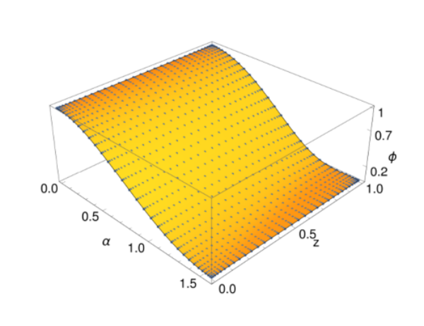
As was discussed in the previous subsection we assume symmetry in variable and use solution of the boundary ODE system as a Dirichlet condition for . The line corresponds to the line . We set there black hole condition with a vanishing scalar field. At the horizon we impose the regularity of the solution following [11]. As in the previous case of zero temperature we use the same spectral methods [31] combined with a scipy nonlinear solver in Python. Sample solutions for are shown in the plot on Fig. 2. We see that the special choice of coordinate system rendered the Dirac delta source well behaved with the solution being regular and showing no anomalies which are present in the case without supersymmetric potential. The geometry smoothly interpolates between the horizon and the delta defect located at the boundary. Surprisingly there is only little dependence on the holographic direction as one goes from the UV to IR where the horizon is located.

While solving (27) numerically we have to make sure that the solution is also a solution to the original Einstein equations. In the pure gravity case one can show that it is indeed true and no Ricci solitons are possible [33]. In the case with matter this question remains open and we checked numerically, that our solutions indeed have .
4.4 Regularized Dirac delta at
To cross-check our numerics we also constructed backreacted geometries corresponding to a set of regularized localized defects, which converge to an exact Dirac delta for a vanishing regulator. In this case we take as a quasi-localized source for the scalar
| (31) |
which is motivated by the linear solution of our problem. Here determines the width of the configuration and in the limit we recover the strict Dirac delta source of the previous sections.
In this case we use a modified version of our coordinates namely we define
| (32) |
so that our source term takes the form
| (33) |
As previously is in the range .
The treatment of boundary conditions is similar to the previous case but for the significant simplification that for the conformal boundary we can now directly impose the source (33) for the scalar and empty metric for the remaining functions.
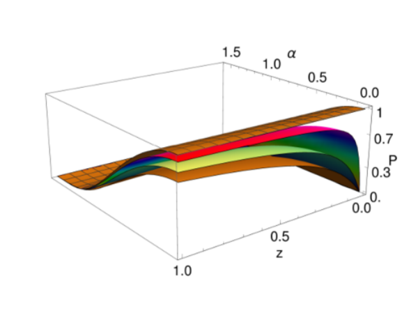

In order to compare the regularized solutions with the backreacted geometries from the previous sections we need to match the relevant parameters which is not completely trivial. The solutions of the exact defect are parameterized by the value of the scalar field at the point and . One recovers the amplitude by an integration of the source term over the conformal boundary
| (34) |
where the last equality comes from the coordinate transformation (32) and the term comes from normalization. This function turns out to have a fixed point for i.e. for that value of the field . In Fig. 3 we see that for smaller and smaller values of the regulator, the results converge to the solution corresponding to the exact Dirac delta defect.
5 Entanglement entropy
Entanglement entropy is an interesting probe of various physical systems, for which there exists a clear holographic prescription due to Ryu and Takayanagi [35, 36] (see [37] for a review). Apart from being of direct physical interest, we will employ entanglement entropy also as an important nontrivial cross-check of our numerical relativity constructions of the backreacted geometries with Dirac delta sources. Namely, we will link the small size limit of the entanglement entropy with the one. Due to the fact that the relevant and background geometries were obtained using quite different methods in qualitatively different coordinate systems, the agreement of these observables will be a nontrivial check of our determination of these backreacted geometries.
According to [35, 36], in a holographic setup the prescription to compute entanglement entropy of some region of boundary CFT is the following: one takes a closed curve inside of which the region of interest lies and then computes the extremal surface (with respect to the bulk metric) whose boundary is the given curve. Then the entanglement entropy is given by the area of that surface. One must proceed with some caution and renormalise the observable, as the conformal boundary lies ’at infinity’ of the bulk space-time and therefore any surface reaching conformal boundary has an infinite area. In the case of various kinds of defects similar calculations of entropy in CFT have already been done [26, 38, 39]. In particular in reference [39] entanglement entropy has been obtained for a number of known defect configurations.
Since our problem admits translational symmetry along the axis we will only be interested in entanglement entropy contained in a strip of boundary theory which has the defect in its center. The first issue one encounters in this calculation is how are curves that reach conformal boundary at some given values of the variable mapped under the coordinate transformation connecting Poincaré coordinates (6) and our slicing ones (8) for the case, or the transformation given by (30) for the black hole case. The two cases need a separate treatment as the employed coordinate systems are different.
5.1 The case
In the case we use the generalized angular coordinate system with a generic rule of transformation to ordinary Fefferman-Graham (FG) patch coordinates , . The functions and are no longer simple trigonometric functions in the backreacted case which poses some complications in the following.
The problem of finding the relevant extremal surface reduces to determining the function which solves the equations of motion following from extremalization of the Nambu-Goto action. The entanglement entropy is then determined by evaluation of the action on the solution. With our assumptions NG action takes the following form
| (35) |
with the resulting equation of motion
| (36) |
Since the integral in the Nambu-Goto (NG) action is clearly UV divergent, one has to perform a cut-off procedure. In order to combine the results both with and without the defect, the regularization has to be done covariantly. This is achieved by always expressing the asymptotic part of the metric in FG coordinates and setting the regulator . This then translates back to the cutoff in new coordinates by the solution of . We thus have to determine, to some degree, the coordinate transformation function .
This can be done by writing, in FG coordinates, the most general form of a metric which is consistent with the symmetries of the problem
| (37) |
Employing now the transformation laws , and comparing with our metric ansatz (11), one obtains
| (38) |
The two integration constants are determined by the requirement that for we get the empty metric which boils down to two conditions
| (39) |
| (40) |
It is important to note, that coordinates (37) do not cover the whole spacetime, since . However, for our purposes, it is enough to consider only the near boundary region, where formulas work fine. There, the transformation can be found perturbatively, in parallel to the expansion of , and it reduces to the ordinary polar coordinates in the absence of the defect, in which case it is regular in the whole range of .
To get the entanglement entropy we now must evaluate the NG action on the solution. Due to translational symmetry along the defect we quote all formulas per unit length in the direction. As it was already mentioned there is a UV divergence coming from a simple pole of at . This part of the integral can be separated and estimated analitically to be
| (41) |
where is a cut-off defined above by . To find the limiting behaviour we can now expand this equation near the boundary to obtain to get the divergent part expressed by a Poincare path regulator
| (42) |
It turns out that for all our solutions , which gives the right UV divergence. The regular part follows conformal invariance so that the total result reads
| (43) |
for some positive which depends on the amplitude of the source.
A surprising feature of the obtained result is that the regularized entanglement entropy is lower than the corresponding one in empty spacetime (see figure 4). Indeed for , a fit to the difference between numerical data and the empty result yields
| (44) |
This is clearly intriguing, although it does not indicate any contradiction, especially as we are not considering here a different state in the original theory but rather a deformation of the theory by a nontrivial source added to the Lagrangian.
5.2 The finite temperature case
The entanglement entropy calculation at nonzero temperature follows the same basic steps as before but with appropriate modifications due to the different coordinate system employed for the background geometry. In this case the corresponding minimal surface will be described by coordinates with a non-trivial dependence . The boundary condition for the surface is where is the half width of the strip. In order for the equations to be regular we adopt the following ansatz
| (45) |
after which the NG Lagrangian takes the following form
| (46) |
where
| (47) | |||||
The equation of motion is a non-linear ordinary differential equation defined numerically in terms of the profiles calculated in section 4. The boundary conditions for the extremal surface translate to: and . The resulting equation with these boundary conditions can be solved using spectral discretization with the Newton method.
In order to evaluate the entanglement entropy we regularize the divergent action, evaluated on-shell, by subtracting pointwise the proper NG Lagrangian evaluated on a corresponding extremal surface in empty , found numerically in an analogous coordinate system on the same numerical grid in i.e.
| (48) |
We calculate the entanglement entropy for a Dirac delta defect characterized by for the (half-)width of the strip the range . The results are shown in figure 5.
Due to the conformal symmetry of the defect the generic form of the entanglement entropy has to be
| (49) |
where is some smooth function. Of course will also depend on the (dimensionless) amplitude of the Dirac delta function. This formula allows for making a connection with the entanglement entropy computation for presented earlier. Indeed, for fixed when we recover the vacuum defect result. For this particular case the falloff has a coefficient which is consistently checked against zero temperature calculation (44). This is also a nontrivial check of our numerical constructions of the relevant backgrounds, as due to the different coordinate systems employed the extremal surfaces for small obtained in both cases are quite different as can be seen on Fig. 6.
It is quite interesting to compare the finite temperature entanglement entropy with and without the defect. The relevant plots are shown in figure 7. Again we observe the rather surprising result that the defect source decreases the entanglement entropy. Clearly, for small the effects of the defect are significant while for thermal effects start to dominate.
6 Conclusions
In this paper we constructed holographic duals of strongly coupled three-dimensional CFT’s deformed by a localized Dirac delta source. The motivation for this work was to move towards a holographic construction mimicking a crystalline lattice with pointlike localized sources. In the present paper we have concentrated on developing the necessary numerical relativity methods in order to consistently handle Dirac delta like sources and considered explicitly a single defect along a line both at zero and at nonzero temperature.
The 1D Dirac delta source for a scalar operator of dimension is scale invariant. We found that requiring that the backreacted geometry respects this scale invariance imposes very stringent constraints on the scalar potential which is consequently uniquely determined. An intriguing outcome is that the resulting potential is exactly the scalar potential appearing in certain Kaluza-Klein reductions of 11D supergravity. All further considerations in the present paper were performed with this concrete choice of the scalar self-interaction.
In order to find the dual backgrounds, we had to use systems of coordinates which were adapted to the presence of the Dirac delta source and which took into account the high variability of the scalar field and of the metric coefficients in the infinitesimal neighbourhood of the point of insertion of the Dirac delta function on the boundary.
At zero temperature, we constructed the dual backgrounds in two ways: using a perturbative expansion and performing a direct numerical solution of the equations of motion using an slicing analogous to the one used for obtaining the Janus solution [19, 27].
For nonzero temperature, we adopted the DeTurck method which required, however, two modifications. Firstly, the adapted choice of coordinates (similar but different from the one that we used for ) was encoded in the choice of coordinates used for the reference black hole metric. Secondly, the boundary at of the numerical grid represented really the infinitesimal neighbourhood of the Dirac delta source and the values of the fields there had to be determined from the equations of motion. With those two modifications in place we constructed the numerical background and performed two cross checks. We compared the resulting numerical background with analogous geometries obtained for regularized delta sources. We also compared the small size limit of entanglement entropy with the entanglement entropy evaluated at zero temperature.
Incidentally, we found that the entanglement entropy evaluated in the theory deformed by the Dirac delta source is lower than the analogous quantity without the defect. It would be very interesting to understand this property from a more physical perspective.
There are numerous directions for further study like the construction of a lattice of Dirac delta defects in order to study phenomena analogous to [11], extensions to chemical potentials and pointlike sources. It would be interesting to determine whether the ‘hovering black hole’ phenomena observed in [17] have their counterpart in the present context. We intend to address at least some of these issues in subsequent work.
Acknowledgements: The authors would like to thank Maciej Maliborski, Hesam Soltanpanahi, Paweł Caputa, Ludwik Turko, Jorge Santos and Przemysław Witaszczyk for discussions. RJ and JJ wish to thank Galileo Galilei Institute for Theoretical Physics for hospitality and the INFN for partial support during the program Holographic Methods for Strongly Coupled Systems where this work was finalized. RJ was partially supported by the Polish National Science Center (NCN) grant 2012/06/A/ST2/00396 while JJ by the NCN post-doctoral internship grant DEC-2013/08/S/ST2/00547.
References
- [1] J. M. Maldacena, “The Large N limit of superconformal field theories and supergravity,” Int.J.Theor.Phys. 38 (1999) 1113–1133, arXiv:hep-th/9711200 [hep-th].
- [2] E. Witten, “Anti-de Sitter space and holography,” Adv.Theor.Math.Phys. 2 (1998) 253–291, arXiv:hep-th/9802150 [hep-th].
- [3] S. Gubser, I. R. Klebanov, and A. M. Polyakov, “Gauge theory correlators from noncritical string theory,” Phys.Lett. B428 (1998) 105–114, arXiv:hep-th/9802109 [hep-th].
- [4] S. A. Hartnoll, “Lectures on holographic methods for condensed matter physics,” Class.Quant.Grav. 26 (2009) 224002, arXiv:0903.3246 [hep-th].
- [5] J. McGreevy, “Holographic duality with a view toward many-body physics,” Adv.High Energy Phys. 2010 (2010) 723105, arXiv:0909.0518 [hep-th].
- [6] A. Donos and J. P. Gauntlett, “Holographic Q-lattices,” JHEP 1404 (2014) 040, arXiv:1311.3292 [hep-th].
- [7] T. Andrade and B. Withers, “A simple holographic model of momentum relaxation,” JHEP 1405 (2014) 101, arXiv:1311.5157 [hep-th].
- [8] B. Goutéraux, “Charge transport in holography with momentum dissipation,” JHEP 1404 (2014) 181, arXiv:1401.5436 [hep-th].
- [9] A. Donos and S. A. Hartnoll, “Interaction-driven localization in holography,” Nature Phys. 9 (2013) 649–655, arXiv:1212.2998.
- [10] A. Donos, B. Goutéraux, and E. Kiritsis, “Holographic Metals and Insulators with Helical Symmetry,” JHEP 1409 (2014) 038, arXiv:1406.6351 [hep-th].
- [11] G. T. Horowitz, J. E. Santos, and D. Tong, “Optical Conductivity with Holographic Lattices,” JHEP 1207 (2012) 168, arXiv:1204.0519 [hep-th].
- [12] M. Rangamani, M. Rozali, and D. Smyth, “Spatial Modulation and Conductivities in Effective Holographic Theories,” arXiv:1505.05171 [hep-th].
- [13] G. T. Horowitz and J. E. Santos, “General Relativity and the Cuprates,” JHEP 06 (2013) 087, arXiv:1302.6586 [hep-th].
- [14] A. Donos and J. P. Gauntlett, “The thermoelectric properties of inhomogeneous holographic lattices,” JHEP 1501 (2015) 035, arXiv:1409.6875 [hep-th].
- [15] Y. Ling, C. Niu, J.-P. Wu, and Z.-Y. Xian, “Holographic Lattice in Einstein-Maxwell-Dilaton Gravity,” JHEP 1311 (2013) 006, arXiv:1309.4580 [hep-th].
- [16] M. Blake, A. Donos, and D. Tong, “Holographic Charge Oscillations,” arXiv:1412.2003 [hep-th].
- [17] G. T. Horowitz, N. Iqbal, J. E. Santos, and B. Way, “Hovering Black Holes from Charged Defects,” arXiv:1412.1830 [hep-th].
- [18] R. de L. Kronig and W. G. Penney, “Quantum Mechanics of Electrons in Crystal Lattices,” Proc. R. Soc. Lond. A 1931 130 (1931) .
- [19] D. Bak, M. Gutperle, and S. Hirano, “A Dilatonic deformation of AdS(5) and its field theory dual,” JHEP 0305 (2003) 072, arXiv:hep-th/0304129 [hep-th].
- [20] E. D’Hoker, J. Estes, and M. Gutperle, “Ten-dimensional supersymmetric Janus solutions,” Nucl.Phys. B757 (2006) 79–116, arXiv:hep-th/0603012 [hep-th].
- [21] A. Clark and A. Karch, “Super Janus,” JHEP 0510 (2005) 094, arXiv:hep-th/0506265 [hep-th].
- [22] E. D’Hoker, J. Estes, and M. Gutperle, “Exact half-BPS Type IIB interface solutions. I. Local solution and supersymmetric Janus,” JHEP 0706 (2007) 021, arXiv:0705.0022 [hep-th].
- [23] E. D’Hoker, J. Estes, and M. Gutperle, “Exact half-BPS Type IIB interface solutions. II. Flux solutions and multi-Janus,” JHEP 0706 (2007) 022, arXiv:0705.0024 [hep-th].
- [24] N. Bobev, K. Pilch, and N. P. Warner, “Supersymmetric Janus Solutions in Four Dimensions,” JHEP 1406 (2014) 058, arXiv:1311.4883 [hep-th].
- [25] M. Suh, “Supersymmetric Janus solutions in five and ten dimensions,” JHEP 1109 (2011) 064, arXiv:1107.2796 [hep-th].
- [26] D. Bak, M. Gutperle, and R. A. Janik, “Janus Black Holes,” JHEP 1110 (2011) 056, arXiv:1109.2736 [hep-th].
- [27] E. D’Hoker, J. Estes, M. Gutperle, and D. Krym, “Janus solutions in M-theory,” JHEP 0906 (2009) 018, arXiv:0904.3313 [hep-th].
- [28] M. Cvetic, M. Duff, P. Hoxha, J. T. Liu, H. Lu, et al., “Embedding AdS black holes in ten-dimensions and eleven-dimensions,” Nucl.Phys. B558 (1999) 96–126, arXiv:hep-th/9903214 [hep-th].
- [29] M. Duff and J. T. Liu, “Anti-de Sitter black holes in gauged N = 8 supergravity,” Nucl.Phys. B554 (1999) 237–253, arXiv:hep-th/9901149 [hep-th].
- [30] M. Duff, “TASI lectures on branes, black holes and Anti-de Sitter space,” arXiv:hep-th/9912164 [hep-th].
- [31] P. Grandclement and J. Novak, “Spectral methods for numerical relativity,” Living Rev.Rel. 12 (2009) 1, arXiv:0706.2286 [gr-qc].
- [32] D. DeTurck, “Deforming metrics in the direction of their Ricci tensors (Improved version),” Series in Geometry and Topology 37 163 (2003) .
- [33] T. Wiseman, “Numerical construction of static and stationary black holes,” arXiv:1107.5513 [gr-qc].
- [34] M. Headrick, S. Kitchen, and T. Wiseman, “A New approach to static numerical relativity, and its application to Kaluza-Klein black holes,” Class.Quant.Grav. 27 (2010) 035002, arXiv:0905.1822 [gr-qc].
- [35] S. Ryu and T. Takayanagi, “Holographic derivation of entanglement entropy from AdS/CFT,” Phys.Rev.Lett. 96 (2006) 181602, arXiv:hep-th/0603001 [hep-th].
- [36] S. Ryu and T. Takayanagi, “Aspects of Holographic Entanglement Entropy,” JHEP 0608 (2006) 045, arXiv:hep-th/0605073 [hep-th].
- [37] T. Nishioka, S. Ryu, and T. Takayanagi, “Holographic Entanglement Entropy: An Overview,” J.Phys. A42 (2009) 504008, arXiv:0905.0932 [hep-th].
- [38] T. Azeyanagi, A. Karch, T. Takayanagi, and E. G. Thompson, “Holographic calculation of boundary entropy,” JHEP 0803 (2008) 054–054, arXiv:0712.1850 [hep-th].
- [39] J. Estes, K. Jensen, A. O’Bannon, E. Tsatis, and T. Wrase, “On Holographic Defect Entropy,” JHEP 1405 (2014) 084, arXiv:1403.6475 [hep-th].