Spatial Process Gradients and Their Use in Sensitivity Analysis for Environmental Processes
Abstract
This paper develops methodology for local sensitivity analysis based on directional derivatives associated with spatial processes. Formal gradient analysis for spatial processes was elaborated in previous papers, focusing on distribution theory for directional derivatives associated with a response variable assumed to follow a Gaussian process model. In the current work, these ideas are extended to additionally accommodate a continuous covariate whose directional derivatives are also of interest and to relate the behavior of the directional derivatives of the response surface to those of the covariate surface. It is of interest to assess whether, in some sense, the gradients of the response follow those of the explanatory variable. The joint Gaussian structure of all variables, including the directional derivatives, allows for explicit distribution theory and, hence, kriging across the spatial region using multivariate normal theory. Working within a Bayesian hierarchical modeling framework, posterior samples enable all gradient analysis to occur post model fitting. As a proof of concept, we show how our methodology can be applied to a standard geostatistical modeling setting using a simulation example. For a real data illustration, we work with point pattern data, deferring our gradient analysis to the intensity surface, adopting a log-Gaussian Cox process model. In particular, we relate elevation data to point patterns associated with several tree species in Duke Forest.
Keywords:
Cauchy Process, Directional Derivative, Gaussian Process, log-Gaussian Cox Process, Matérn Correlation Function1 Introduction
Increasingly, data is being collected at geo-referenced locations. For a region of interest , the set of conceptual responses can be viewed as a realization of a random surface, observed at a finite set of locations. While covariate information may explain a substantial portion of the variation in response, there is often underlying spatial structure that is difficult to measure. Inference on this spatial structure can be made via the parameters in a spatial process model. Under these models, prediction at unobserved locations, or kriging, is possible, enabling interpolation across the region.
Spatial regression models commonly assume a linear relationship and make inference based on the coefficient assigned to the covariate. This coefficient describes the expected change in response given a unit change in covariate, thus providing a global measure for the sensitivity of the response to the covariate. However, it is expected that the relationship between the variables may vary locally over the study region. Such local, or second-order, behavior can be studied through spatial sensitivity or gradient analysis.
A spatial gradient analysis will enable spatial examination of a response variable’s sensitivity to a covariate across the region of interest. The sensitivity of the response variable may vary based on the rate of change for the covariate or due to additional unaccounted for factors, resulting in areas where the relationship appears weaker or stronger. Models allowing for spatially varying coefficients, such as Fotheringham et al. (2002); Gelfand et al. (2003), provide some similar inference but assume a more complex model structure. The methodology proposed here assumes a standard spatial linear regression model but provides a post model fitting framework for examining the variation in the response’s sensitivity to the covariate.
In ecology such sensitivities are typically discussed when relating plant characteristics to climate. For instance, researchers are increasingly interested in characterizing how abundance and frequency of tree species relate to changes in variables such as temperature and precipitation, in order to learn about the expected effects of climate change on range distributions (Thuiller et al., 2004; Canham and Thomas, 2010; Thomas, 2010, e.g.). These analyses focus on a comparison of sensitivities across species, while little consideration is given to how sensitivities may vary spatially within a given species. Our approach is aimed at the latter question.
The interpretation of the coefficient in a spatial regression as a global gradient, , inspires consideration of local sensitivities through directional derivative processes, or spatial gradients. Spatial gradients under Gaussian processes were elaborated by Banerjee et al. (2003b) to address the rate of change of a spatial surface at a given point in a given direction. Their paper defines directional derivative processes with corresponding distribution theory to enable interpolation across a region. The gradient distributions are fully determined by the spatial model parameters, allowing all gradient analysis to occur post model fitting. Distributions for derivatives of Gaussian processes have also been discussed in the context of observed derivatives of functions (O’Hagan, 1992; Solak et al., 2003, e.g.), as well as for random fields more generally Adler (1981). In all of the previous work with Gaussian process directional derivatives (Banerjee and Gelfand, 2003; Banerjee and Gelfand, 2006; Majumdar et al., 2006, e.g.), the researchers have considered the rates of change of a response surface with the mean surface modeled as a linear function of a set of fixed covariates. In contrast, to accommodate the desired spatial sensitivity analysis, we will assume a single covariate of interest whose surface is spatially smooth such that it too can be treated as a realization of a stochastic process. The behavior of the response and covariate processes, as well as their associated derivative processes, are then considered jointly and functions of these derivatives can be explored.
The contribution of this paper is to extend the existing spatial gradient theory to accommodate spatial sensitivity analysis by modeling the response and covariate jointly. Working within a hierarchical Bayesian modeling framework, corresponding gradients for the spatial surfaces can be sampled simultaneously from the joint predictive distribution post model fitting. Under a significant regression relationship it is not sensible to investigate the gradient behavior of the surfaces marginally. Suitable comparison between the gradient surfaces illustrates how sensitive the response surface is to the covariate surface, as well as the strength of this relationship. The former is accomplished through comparison between the directions of the maximum gradient at a given location; the latter requires consideration of their directional derivatives relative to one another. In particular, we introduce two new spatial processes, a local directional sensitivity process and a spatial angular discrepancy process. These inferential tools are developed and carried out on simulated data in the context of a customary geostatistical model Banerjee et al. (2003a); Cressie and Wikle (2011) as well as with an ecological dataset where we connect point patterns of trees with elevation.
In Section 2 the formal distribution theory for the spatial gradients is extended to the multivariate case. Section 3 outlines the modeling framework for our examples. This section also defines the two processes of interest, namely the local directional sensitivity process and the spatial angular discrepancy process. Section 4 provides a simulated example with a multivariate Gaussian process setup as a proof of concept. Section 5 provides an analysis of point pattern data from Duke Forest, extending the analysis techniques to a non-Gaussian response; the intensity of the point pattern, modeled using a log-Gaussian Cox process, is explored by employing a spatial gradient chain rule. Finally, Section 6 summarizes the contributions of the paper and suggests future work.
2 Distribution Development
In this section we review the definitions and distributions presented in Banerjee et al. (2003b) and extend these ideas to consider a multivariate Gaussian process. We assume locations , 2-dimensional Euclidean space, however extension to a generic -dimensional setting is straightforward. The process is assumed, for convenience, to be (weakly) stationary such that the covariance function, , depends only on the separation vector . In fact, in our examples we adopt isotropic covariance functions that depend only on the length of the separation vector, .
Consider two surfaces drawn from a joint Gaussian process specified such that has constant mean, say , and covariance function . Given , has mean and covariance function . Observed at a set of locations , we write: with . Considered jointly, we have:
where and are matrices of the covariance functions with entry evaluated at .
We follow the notation and theory in Banerjee et al. (2003b). Suppose mean square differentiable processes and . That is, for , at there exists a vector such that for any scalar and any unit vector , where in the sense as . Similarly, for .
In particular, define the finite difference processes at scale in direction :
where is a unit vector. Taking the limit as tends to 0, Banerjee et al. (2003b) define the directional derivative processes in the direction :
where is the vector of directional derivatives in the orthonormal basis directions and for . We can study the directional derivative processes for any by working with the basis set and .
From Banerjee et al. (2003b), we know that if and are stationary Gaussian processes, then the resulting marginal distributions involving the directional derivatives will be stationary Gaussian processes as well. Note, isotropy in the process does not induce isotropy in the process; only stationarity will be inherited. Similar to the discussion in their paper, we know by linearity that will be a stationary multivariate Gaussian process. And then, by a standard limiting moment generating function argument, will also be a stationary multivariate Gaussian process.
To explicitly provide the joint distribution, we derive the cross covariance structure by examining pair-wise covariances between the response and covariate processes and their directional derivatives. For notational convenience, write the marginal covariance function of to be . Assume the and processes are mean zero, setting , since in practice the gradients are calculated for the mean zero residual process. If , then , so the joint processes will all be mean zero. We calculate the covariances associated with the directional derivatives by taking the limits of the covariances corresponding to the analogous finite difference process.
The covariances for the response surface are derived in Banerjee et al. (2003b):
and covariances for the covariate surface are analogous:
To fully describe the joint distribution we derive the covariances between response and covariate surfaces similarly:
where and .
Relationships between the response surface, the covariate surface and their corresponding directional derivative surfaces can be described through the 6-dimensional multivariate stationary Gaussian process . Using the covariances calculated above, the associated cross-covariance matrix for will be:
where is a gradient vector associated with , and is the Hessian matrix associated with .
For , we have a block diagonal local covariance matrix:
Thus, at a location , the directional derivative surfaces will be correlated with one another, but neither will be correlated with either of the data surfaces. Intuitively, this makes sense since we would not expect the level of the surface at a location to be correlated with the rate of change at that location. Of course, since is a bivariate Gaussian process, the correlation between the rates of changes is not surprising.
The Matérn covariance is adopted below. It depends on a smoothness parameter which directly controls the mean square differentiability of process realizations Stein (1999). This is convenient since, again, the and processes must be mean square differentiable for their associated directional derivative processes to be well defined. If we let and be Matérn with then they are once (but not twice) mean square differentiable, and, if , the covariance functions are of the closed form . We denote the parameters of as and , and the parameters of as and .
Under the Matérn covariance the components of the cross-covariance matrix will be , , , and similar for . Then, we have for :
where is the identity matrix. As above, and will be correlated with one another, and similarly and will be correlated with one another, but all other pairings of the directional derivatives will be uncorrelated.
3 Model Fitting and Inference
3.1 Sampling Method
Following the modeling of the previous section, let and , where the and are valid two-dimensional correlation functions. We work with the Matérn class of covariance functions parameterized by and with .
Let . For locations , the overall likelihood can be written in terms of the conditional likelihoods
where , and . The likelihood could be equivalently written in its joint form, but the conditional form is more conducive to interpreting and implementing the gradient analysis.
We see that we have a low dimensional parametric model, with only dimensional. We utilize fairly non-informative priors for its components. For example, vague normal priors on , vague inverse Gamma priors on , vague Gamma priors on , and priors on . The prior on follows the suggestion of Stein (1999) and others who observe that distinguishing from would be very difficult in practice. This model is straight forward to fit in its conditional form, for example using the ‘spBayes’ package in R Finley et al. (2007). Thus, assume we now have posterior samples , from .
Once we have posterior samples of the parameters, we draw samples of the gradient vectors using composition since the posterior predictive distribution . The cross-covariance matrix derived earlier allows us to immediately write the joint multivariate normal distribution given , which can be evaluated at each sample . Based on this joint distribution, standard multivariate normal theory allows us to write down the desired conditional distributions needed to draw from the predictive distribution.
For an unobserved location , obtaining draws of the gradient vectors is again done via the predictive distribution. The cross covariance matrix derived enables us to write the joint distribution, from which we can derive the conditional distribution . If interest is also in the values of the and surfaces at the new location, we would derive the conditional distribution , which is again straight forward given the cross covariance matrix and allows joint prediction of the surfaces and their gradients at the new location.
If we want and to be adjusted based on some fixed covariates, then we simply introduce such covariates into the mean functions of the model. We create a spatial random effects model:
where and are vectors of covariates used to explain the and surfaces respectively, with coefficients and ; and are independent mean-zero stationary Gaussian processes with parameters as before; and is a Gaussian white-noise process with variance intended to capture measurement error or microscale variability in the response. The process is assumed to be a fully spatial model (no nugget effect), such as might be used for elevation, temperature, or pollutant level.
With now extended to , the likelihood for locations above can be trivially revised.
Prior selection for the parameters will be similar to the previous example. Again, this model can be implemented using ‘spBayes’, and draws of the gradients will rely on the posterior predictive distribution, which can be calculated as before using the derived cross-covariance matrix.
3.2 Local Directional Sensitivity Process
At a given location there may additionally be interest in the ratio of directional derivatives, , corresponding to the relative rates of change in the two surfaces in direction . This quantity is analogous to in more standard calculus applications as well as sensitivity functions studied in sensitivity analysis Tomovic and Vukobratovic (1972). With this in mind, we refer to the resulting spatial process as the local directional sensitivity process. The choice of will depend on the application being considered. For example, this direction may correspond to latitudinal direction, an elevation direction, or to an environmental feature expected to impact the response. Large values of this process would suggest that the change in covariate surface has a high impact on the the response surface.
The joint process defined in Section 2 can be equivalently represented as a spatial random effects model (excluding nugget effects):
where and are independent processes. With this notation we can write the unconditional response surface and corresponding directional derivative process as follows:
The local directional sensitivity process can then be written
| (5) |
We see that the multiplicative parameter, , defining the overall relationship between the and processes serves to center the local directional sensitivity process.
As mentioned in Majumdar et al. 2006, if we consider , then one could write ; i.e., is describing the rate of change in relative to changes in . Again, at any location the directional derivative ratio will be centered at the global (non-directional) derivative ratio plus some (directional) spatial noise. In this way, the directional derivative ratio process is describing the spatial variation in the relative rates of change between and . This is analogous to modeling adopting spatially varying coefficients, , Gelfand et al. (2003) but is arguably a simpler context since the derivatives require no additional model fitting. In addition, consideration of directional perspectives using this gradient approach allows for inference distinct from what one can learn from a non-directional parameter.
By noting that is a ratio of independent mean zero normal random variables, at each location the directional spatial noise is a Cauchy random variable with scale equal to the ratio of the respective standard deviations, . If , then . If is isotropic, then Banerjee et al. (2003b) and . If and are Matérn with , then , and the scale for the Cauchy distribution will be . When the respective standard deviations are equal, the scale will be 1 and the directional derivative ratio will have a standard Cauchy distribution.
In fact, the collection of directional derivative ratios form a well defined spatial stochastic process which would naturally be called a spatial Cauchy process (see Appendix A for details). For any set of locations the joint distribution is well defined. For example, consider two locations and , simplifying the notation for clarity:
In turn, each of these terms can be computed as an integral involving normal densities. For example, the first term can be written as follows:
| (6) |
where is the bivariate normal density for the Gaussian process with parent covariance function evaluated at and , and similar for . Recall that a univariate Cauchy distribution can be defined as a scale mixture of normals Andrews and Mallows (1974). If we write the corresponding CDF as , then the form in Equation 6 is evidently similar and can be regarded as a bivariate analogue. In this way, the spatial Cauchy process is defined such that at any location the distribution is a univariate Cauchy distribution and for any set of locations the distribution is a sum of integrals of a similar form.
In the data analysis examples we consider a fixed direction and draw samples of the directional derivative ratio at each location across a region. Although we cannot show mean square continuity for this surface, by imposing additional smoothness conditions on the covariance functions for and , we can argue that this surface will be almost surely continuous using results from Kent (1989), following the development in Banerjee and Gelfand (2003). We omit the details.
3.3 Spatial Angular Discrepancy Process
At any given location there may be interest not only in the magnitude of the gradients in various directions, but also in the direction at which the maximum gradients are achieved. Stronger alignment between the directions of maximum gradients would suggest a stronger relationship between the response and covariate surfaces.
Consider the covariate process . At location the maximum gradient will be achieved in the direction described by the unit vector , and the directional derivative in the direction of maximum gradient will be Banerjee et al. (2003b). We can similarly consider the direction of maximum gradient for the response surface which will occur for . In applications, researchers may be interested in the behavior of the response surface, or its relative rate of change, in the direction . That is, there may be interest in as well as .
At a location the magnitude of the maximum gradient, , will be the square root of a sum of squared independent normal random variables; as such, this quantity will have a Chi distribution with degrees of freedom, possibly scaled by some factor. If the process is isotropic, then will have a Chi distribution with degrees of freedom scaled by . For the Matérn covariance () structure this scaling factor will be equal to .
The unit vector describing the direction of max gradient for the covariate surface can equivalently be described by an angle such that , and similarly for the response surface. The angle can take values from to , so inversion of tan must be done with care. Since tan has a period of only , the inverse function is typically taken to be arctan∗. 11 1 arctan is arctan if , ; if , ; arctan if ; arctan if , ; and undefined if , Jammalamadaka and Sengupta (2001).
As smooth functions of a well defined spatial process, the directions of maximum gradient define a bivariate projected Gaussian process, analogous to the univariate projected Gaussian processes described in Wang (2013). Marginally and will each be a projected Gaussian process Wang (2013). Assuming the Matérn () covariance structure we can derive the joint distribution of the two angles at a given location :
where , , , , , and is the zero mean bivariate normal cdf with correlation and standard deviations equal to 1 evaluated at . A brief derivation is provided in Appendix B. In addition, it is straightforward to show that at each location the angles, and , will marginally be uniform on .
The above bivariate density is plotted in Figure 1 for , holding all other parameters constant: and . When the mass is concentrated around pairs that are equal; when the mass is concentrated around pairs where . When the relationship between and is weak, and the density is roughly uniform over all angle pairs. As the magnitude of increases, the mass becomes increasingly concentrated around these respective values.

To compare the directions of maximum gradient calculated from the posterior distribution, we compute a “discrepancy” for and . Define: . As a smooth function of a spatial process, this discrepancy is a well defined spatial process which we refer to as the spatial angular discrepancy process. When the maximum gradients occur in identical directions this process will have a value of zero, when they occur in opposite directions the process will have a value of two. In our analyses we consider the process across a region, plotting the posterior median surface.
In some areas the or surface may be quite flat and there will be no direction with a gradient magnitude substantially larger than in the other directions. In these areas a large angular discrepancy may not be as meaningful as it would be in areas with larger gradient magnitudes. For this reason it is useful to examine these plots in tandem with plots of the local directional sensitivity process described in Section 3.2.
3.4 Extensions to Non-Gaussian Data Models Using the Chain Rule
One can imagine modeling scenarios where the response will be non-Gaussian, for instance, binary or zero-inflated data. In these cases, a latent Gaussian surface may be utilized and spatial gradients can still be considered. The resulting gradient surfaces will be for the latent Gaussian process, not necessarily the response of interest; however, differentiable transformations will allow for inference on the non-Gaussian response surface. Recall the chain rule result presented in Majumdar et al. (2006): for differentiable on and , the directional derivative exists and is given by . Here is the latent Gaussian surface and the function describes its relationship to the non-Gaussian response of interest.
When analyzing the Duke Forest data in Section 5, we work with a log-Gaussian Cox process model for the intensity surface. To study gradients associated with the intensity surface itself, we can use the fact that, if is our response and , then .
In the case of binary data we can write a model with response if and if , where is a latent Gaussian process centered at a linear function of a spatial covariate . We have a spatial probit regression since Heagerty and Lele (1998). There may be interest in identifying areas where the transition between regions of high absence probabilities to regions of low presence probabilities is rapid (or vice versa). Consideration of the local directional sensitivity process associated with the probability surface and the covariate surface would provide an avenue to answer these kinds of questions. Now, with the function , we obtain .
4 Simulation Example
We consider a simulation example to explore the behavior of gradient quantities in a controlled setting. From the foregoing development, in the context of spatial gradient analysis the quantities of interest will be directional derivatives. These derivatives are unobservable even in a simulation study with known parameters. Thus, assessing inference performance with regard to these quantities requires some novelty.
Recall that the gradient processes describe the shape and behavior of spatial surfaces. With a simulated dataset, we are able to draw a realization of the Gaussian process over a larger number of locations, allowing for fairly detailed understanding of the spatial surfaces. To avoid any unfair advantage that might come from the increased sample size, we use only a subset of the locations to fit the model and reserve the full set of locations for assessing the quality of our inference. Contour lines highlighting the shape of the surface are interpolated using the full set of locations. Conclusions made using gradients are then compared to those suggested by the contour lines to examine performance.
4.1 Data and Model
We simulate a realization from a mean zero Gaussian process on , and a realization from a Gaussian process with mean . We use Matérn covariance functions setting in order to capitalize on the resultant closed form. We simulate the Gaussian processes assuming Matérn covariance functions with parameters , , , and . We draw a larger realization at 2000 locations, to allow for finer knowledge of the underlying surface, from which we consider a subset of 200 locations to be our “observations”.
Treating as a multivariate Gaussian process, we fit a coregionalization model using the conditional parameterization, as described in Section 2. The model is fitted using the ‘spbayes’ package in R by first fitting parameters for , then fitting parameters for . We obtain 2000 samples after a burn-in of 500 iterations and a thinning of every fifth iterate. We assume . Priors for the remaining parameters are: where and . Summaries of the posterior parameter samples are provided in Table 1.
| Parameter | 0.025 | Mean | 0.975 | Truth |
|---|---|---|---|---|
| -0.7126 | -0.0614 | 0.6214 | 0 | |
| 0.2726 | 0.8179 | 1.3867 | 0 | |
| 0.4685 | 0.5943 | 0.7202 | 0.5 | |
| 0.6725 | 1.0692 | 1.7390 | 1 | |
| 0.8242 | 1.0230 | 1.2124 | 1.05 | |
| 0.4911 | 0.8057 | 1.3341 | 1 | |
| 0.8572 | 1.0718 | 1.3116 | 1.05 |
We consider a region centered at the location . The and values at this location are provided in Figure 2. (The full processes were realized on , but we only show a subregion here.) The interpolated surface and contour lines are produced using the full 2000 locations, while the circles indicate the subset of 200 locations used to predict the gradient.

4.2 Local Directional Sensitivity Process
We are interested in the behavior of . We consider and . Since Banerjee et al. (2003b), any discussion of the behavior in direction implies the opposite behavior is occurring in the opposite direction. When applied to the ratios, this means that the local directional sensitivity process will be equal for and .
Returning to the region in Figure 2, to visualize the local directional sensitivity process we draw samples at a grid of 125 locations denoted as . We draw 2000 samples of from the joint predictive distribution, again, given the fitting data at 200 observed locations. For each of these samples we calculate . We summarize the central behavior of these Cauchy quantities at a given location using the median value of the ratios.
For the two directions being considered, we plot the median predictive surface in Figure 3. Interpretation of these surfaces requires examination of the sign of the ratio as well as the magnitude. Magnitudes less than 1 suggest that the surface is changing more rapidly than the surface; magnitudes greater than 1 suggest that the surface is changing more rapidly than the surface; negative values suggest that one surface is increasing while the other decreases; positive values suggest that both surfaces are either increasing or decreasing.
The direction points towards the east. The corresponding ratio surface is provided in the left hand plot of Figure 3. There is a peak in the ratio surface around (6.75,6.25), suggesting that both surfaces are either decreasing or increasing and that the surface is doing so more rapidly. Referring back to Figure 2, the contour lines indicate that both surfaces are increasing at that location looking east, and that the surface is doing so more rapidly. The direction points towards the north. The corresponding ratio surface is provided in the right hand plot of Figure 3. There is a peak in the ratio surface around (8.75, 6), suggesting that both surfaces are either decreasing or increasing and that the surface is doing so more rapidly. Referring back to Figure 2, the contour lines indicate that both surfaces are increasing at that location looking east, and that the surface is doing so more rapidly.

4.3 Spatial Angular Discrepancy Process
Consider again the region in Figure 2 and the grid of 125 locations denoted as . Sampling gradients from the joint predictive distribution for , we calculate the direction of maximum gradient as and for each sample gradient at each location in the figure. Denote these angles (in radians) as and respectively.
We compute the discrepancy between these angles at each location as in Section 3.3 and provide the posterior median values in Figure 4. Most of the region has an associated distance of 0, suggesting that both and are typically increasing most rapidly in the same direction. However, there are a few small regions where the distance peaks towards a value of 2, locations where the and surfaces are increasing in nearly opposite directions.

5 Duke Forest Point Pattern, Elevation Example
5.1 Data
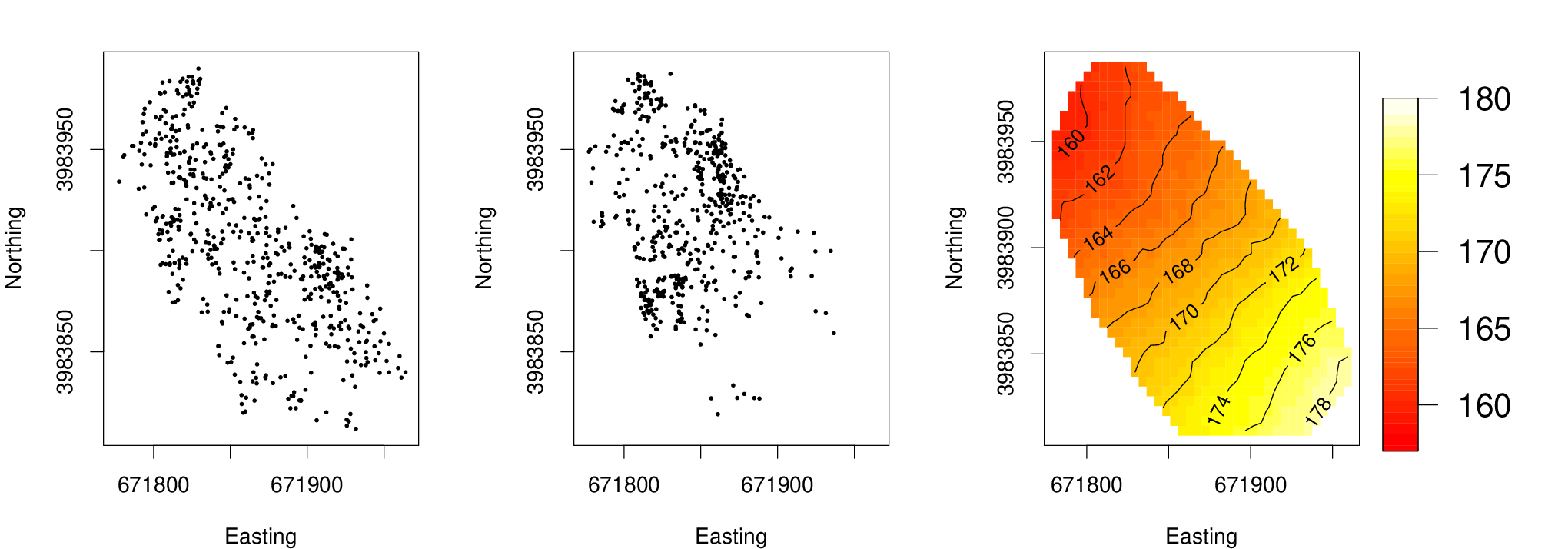
Our illustrative data set is a collection of point patterns of tree species present at the Blackwood site in the Duke Forest in Durham, NC. The site is 5 hectares in area and exhibits a range of elevation. A road and powerline separate the site into three subregions, and we focus on the northwestern of these subregions. We consider two tree species, Flowering Dogwood (Cornus florida) and Sweetgum (Liquidambar styraciflua), with regard to their respective point patterns of locations within the site in the year 2000. Some trees have multiple stems observed at a single location; however we treat these as a single observed tree at the given location. The point pattern for Sweetgum consists of 531 trees, and the point pattern for Flowering Dogwood consists of 570 trees. Elevation is recorded at each location where a tree of any species was observed, resulting in 5654 elevation observations.
Figure 5 provides a heatmap of the elevation data. There is a clear increase in elevation across the region in a roughly southeastern direction. Figure 5 also provides the observed point patterns for each of the species. Flowering Dogwood is well dispersed across the entire region while Sweetgum is more abundant in the northwestern half of the region.
5.2 Point Pattern Model given Elevation
Given the observed elevation, , we model the intensity for each species as a log-Gaussian Cox process: , , and . Placing priors on the parameters, we have the following model:
where is the observed point pattern and is equivalently considered using .
We approximate the likelihood by dividing the region into a fine grid with cells . This gives us the likelihood
where corresponds to a realization from a Gaussian process evaluated at a representative point in each grid cell . This likelihood can be sampled using elliptical slice sampling, as described in Murray et al. (2009) and Murray and Adams (2010).
5.3 Conditional Bivariate Model
In terms of , we immediately have a conditional bivariate GP model with elevation: and with and . Hence, we are in the framework developed above and can apply the proposed gradient analyses. The difference in this case will be that the Gaussian response is latent and thus unobserved. The uncertainty about is propagated through the model by drawing a posterior sample of the surface for each posterior sample of the parameters.

Table 2 provides the fitted parameter values for elevation. Tables 3 and 4 provide the fitted parameter values for each of the species. Note that the parameter is fixed at the minimum contrast estimate, as suggested in Møller et al. (1998), to facilitate identifiability in the fitting of the log-Gaussian Cox process. The fixed values are and 0.0434 for Flowering Dogwood and Sweetgum respectively. The 95% credible interval for contains zero for Flowering Dogwood, but not for Sweetgum. This negative coefficient suggests that the intensity of Sweetgum decreases as elevation increases, while the intensity of Flowering Dogwood is not responsive to elevation changes at this scale. Figure 6 provides the posterior median intensity for each of the species. Both intensities have fairly low values across most of the domain, with a few regions of higher intensity.
| Parameter | 0.025 | Mean | 0.975 |
|---|---|---|---|
| 166.1043 | 167.8577 | 169.4328 | |
| 7.1681 | 9.4117 | 12.9494 | |
| 0.0791 | 0.0892 | 0.0979 |
5.4 Local Directional Sensitivity Process
| Parameter | 0.025 | Mean | 0.975 |
|---|---|---|---|
| -3.6416 | -3.5478 | -3.4590 | |
| -0.0866 | -0.0284 | 0.0348 | |
| 0.3367 | 0.5237 | 0.7648 |
| Parameter | 0.025 | Mean | 0.975 |
|---|---|---|---|
| -4.2161 | -4.0297 | -3.8728 | |
| -0.4094 | -0.2619 | -0.1024 | |
| 0.7942 | 1.2652 | 1.9160 |
The methods developed in previous sections allow for straight forward examination of , although interest is more likely in the behavior of the intensity surface itself. Applying the spatial gradient chain rule discussed in Section 3.4 gives us , with the directional derivative ratio . As before, we can simplify this in terms of the independent Gaussian processes:
As before, will center the Cauchy random variable, but now there will also be scaling according to the value of .
In Figure 5 we saw a clear increase in elevation in a roughly southeastern direction. We approximate this direction by the unit vector . Again, via the chain rule, we can consider the behavior of the directional derivative ratios in this direction for each of the species. Figure 7 plots the resulting posterior median surfaces.
For Flowering Dogwood the majority of the domain has a ratio close to zero. This suggests that the changes in the intensity are negligible compared to the changes in elevation. Recalling the fairly even spread of the trees in the region, as well as the non-significant , this pattern makes sense.
For Sweetgum, virtually the entire region has a negative directional derivative ratio. This aligns with our interpretation of the significantly negative coefficient, namely that as elevation increases the intensity decreases. There are a few subregions where the change in intensity occurs more rapidly than elsewhere, and there is a larger subregion where the change in intensity is zero due to an absence of trees. The cause for subregions of rapid change could be further illuminated through examination of other factors in those regions. Similarly, the region of zero change in intensity could be roughly interpreted as Sweetgum having an aversion to elevations beyond a certain value.

5.5 Spatial Angular Discrepancy Process
Finally, we can compare the intensity and elevation surfaces by computing the discrepancy between their directions of maximum gradient at each location, i.e., the posterior median of across the region. Values close to 2 suggest the surfaces are most rapidly increasing in opposite directions; values close to 0 suggest the surfaces are most rapidly increasing in the same direction. The posterior median discrepancy surfaces are provided in Figure 8 for Flowering Dogwood and Sweetgum.
The discrepancies for Flowering Dogwood roughly range between 0.8 and 1.5. There is no clear pattern, which supports there being no strong relationship between Flowering Dogwood intensity and elevation.

The pattern for Sweetgum is quite different. All of the discrepancies appear to be between 1.5 and 2, with most around 1.9. This suggests that the Sweetgum intensity and elevation are increasing in nearly opposite directions virtually everywhere in the domain. This again confirms the negative relationship, and additionally highlights this pattern as being slightly weaker in the northern part of the region.
6 Summary and Conclusions
We have developed methodology for performing spatial sensitivity analysis for a bivariate process where one variable is treated as a response to the other variable. Consideration of the associated directional derivatives can be done jointly and results in a multivariate Gaussian process directly derivable from the model for the parent process fit in a Bayesian framework. Utilizing the posterior draws of the process parameters, all gradient analysis occurs post model fitting.
Using the directional derivatives, we proposed two derived processes in order to learn about the relationship between the response and covariate processes. The first is the local directional sensitivity process, inspired by quantities explored in standard sensitivity analysis. This process captures local variation in the relationship between the two variables and provides deeper insight into their relative behavior across the region. The second is the spatial angular discrepancy process, capturing the discrepancy between the directions in which the process surfaces are most rapidly increasing. Spatial plots of this discrepancy surface highlight regions of the domain where the two processes behave most similarly and most differently, again informing on the variables’ spatial relationship.
Our application involved elevation data and point patterns of trees collected from the Duke Forest. Using a log-Gaussian Cox process, we studied local directional sensitivity of the intensity to elevation through the use of a spatial gradient chain rule. Through the two tree species, this example illustrates the different results one would expect from a spatial sensitivity analysis when the variables are significantly related versus when they are not.
The current theory provides opportunity for several extensions and applications. Many ecological data sets are observed at multiple time points, in part to see if the relationships between the variables of interest are changing over time. With this in mind, future work on gradient analyses may involve the incorporation of temporal effects. Ecological data sets can also have multiple responses such as leaf traits that are being related to multiple climate covariates (Thuiller et al., 2004, e.g.), any or all of which may have relationships that could be better highlighted through a spatial gradient analysis under a joint model. Finally, the spatial gradient chain rule will allow us to consider novel non-Gaussian responses modeled through latent Gaussian process models as described in Section 3.4.
Appendix A
We show that is a well defined spatial stochastic process.
First consider two locations and . For notational convenience, let , , , and . We can write the joint distribution of the ratios in terms of the joint distributions for the two Gaussian processes:
The above joint distribution depends only on integrals of multivariate normal densities, so consistency across permutations of the labels is clearly satisfied.
At a single location the directional derivative ratio is a ratio of two independent normal random variables. As such, it will have a Cauchy distribution with a scale parameter dependent on the parameters in the covariance functions and , namely . Next we show that marginalizing the bivariate distribution over will reduce to the known distribution for the univariate case:
We can then rewrite this as:
The associated density will then be , which was shown in Andrews and Mallows (1974) to be a Cauchy distribution. In this case we will have a Cauchy with scale parameter , as desired.
The marginalization is straight forward for larger dimensions with marginalization over the two normal densities occurring in a similar way.
Appendix B
We are interested in the marginal behavior of at a location where
,
, and
are
normally distributed with the covariance structure provided in
Equation 1.
After converting to polar coordinates, the change of variables formula gives the following integral, where is the multivariate normal density associated with . For clarity we suppress the index :
where , , , , and is the zero mean bivariate normal cdf with correlation and standard deviations equal to 1 evaluated at .
Several integration steps were treated as the expected value of a truncated normal distribution. An additional integration step required integration by three parts, then computation of the probability that the sum of a normal and a truncated normal are less than some constant. This probability was available in closed form in the query by Lipow et al. (1964) and is written in terms of the bivariate normal cdf. Somewhat simplified, this gives the density provided in the text:
Acknowledgements
This research was supported in part by NSF DEB 0842465 and NSF CDI 0940671. The authors thank Thomas J. Leininger for computational assistance and James S. Clark for providing data and giving insight into the underlying ecological processes.
References
- Adler (1981) Adler, R. J., 1981. The geometry of random fields. Vol. 62. Siam.
- Andrews and Mallows (1974) Andrews, D. F., Mallows, C. L., 1974. Scale mixtures of normal distributions. Journal of the Royal Statistical Society. Series B (Methodological), 99–102.
- Banerjee and Gelfand (2003) Banerjee, S., Gelfand, A., 2003. On smoothness properties of spatial processes. Journal of Multivariate Analysis 84 (1), 85–100.
- Banerjee and Gelfand (2006) Banerjee, S., Gelfand, A. E., 2006. Bayesian wombling: Curvilinear gradient assessment under spatial process models. Journal of the American Statistical Association 101 (476), 1487–1501.
- Banerjee et al. (2003a) Banerjee, S., Gelfand, A. E., Carlin, B. P., 2003a. Hierarchical modeling and analysis for spatial data. Crc Press.
- Banerjee et al. (2003b) Banerjee, S., Gelfand, A. E., Sirmans, C., 2003b. Directional rates of change under spatial process models. Journal of the American Statistical Association 98 (464), 946–954.
- Canham and Thomas (2010) Canham, C. D., Thomas, R. Q., 2010. Frequency, not relative abundance, of temperate tree species varies along climate gradients in eastern north america. Ecology 91 (12), 3433–3440.
- Cressie and Wikle (2011) Cressie, N., Wikle, C. K., 2011. Statistics for spatio-temporal data. John Wiley & Sons.
- Finley et al. (2007) Finley, A. O., Banerjee, S., Carlin, B. P., 2007. spbayes: an r package for univariate and multivariate hierarchical point-referenced spatial models. Journal of Statistical Software 19 (4), 1.
- Fotheringham et al. (2002) Fotheringham, A. S., Brunsdon, C., Charlton, M., 2002. Geographically weighted regression. Wiley New York.
- Gelfand et al. (2003) Gelfand, A. E., Kim, H.-J., Sirmans, C., Banerjee, S., 2003. Spatial modeling with spatially varying coefficient processes. Journal of the American Statistical Association 98 (462), 387–396.
- Heagerty and Lele (1998) Heagerty, P. J., Lele, S. R., 1998. A composite likelihood approach to binary spatial data. Journal of the American Statistical Association 93 (443), 1099–1111.
- Jammalamadaka and Sengupta (2001) Jammalamadaka, S. R., Sengupta, A., 2001. Topics in circular statistics. Vol. 5. World Scientific.
- Kent (1989) Kent, J. T., 1989. Continuity properties for random fields. The Annals of Probability 17 (4), 1432–1440.
- Lipow et al. (1964) Lipow, M., Mantel, N., Wilkinson, J., 1964. Query 2: The sum of values from a normal and a truncated normal distribution (continued). Technometrics 6 (4), 469–471.
- Majumdar et al. (2006) Majumdar, A., Munneke, H. J., Gelfand, A. E., Banerjee, S., Sirmans, C., 2006. Gradients in spatial response surfaces with application to urban land values. Journal of Business & Economic Statistics 24 (1).
- Møller et al. (1998) Møller, J., Syversveen, A. R., Waagepetersen, R. P., 1998. Log gaussian cox processes. Scandinavian Journal of Statistics 25 (3), 451–482.
- Murray and Adams (2010) Murray, I., Adams, R. P., 2010. Slice sampling covariance hyperparameters of latent gaussian models. arXiv preprint arXiv:1006.0868.
- Murray et al. (2009) Murray, I., Adams, R. P., MacKay, D. J., 2009. Elliptical slice sampling. arXiv preprint arXiv:1001.0175.
- O’Hagan (1992) O’Hagan, A., 1992. Some bayesian numerical analysis. Bayesian statistics 4, 345–363.
- Solak et al. (2003) Solak, E., Murray-Smith, R., Leithead, W., Leith, D., Rasmussen, C., 2003. Derivative observations in gaussian process models of dynamic systems. Advances in Neural Information Processing Systems 15.
- Stein (1999) Stein, M. L., 1999. Interpolation of spatial data: some theory for kriging. Springer.
- Thomas (2010) Thomas, C. D., 2010. Climate, climate change and range boundaries. Diversity and Distributions 16 (3), 488–495.
- Thuiller et al. (2004) Thuiller, W., Lavorel, S., Midgley, G., Lavergne, S., Rebelo, T., 2004. Relating plant traits and species distributions along bioclimatic gradients for 88 leucadendron taxa. Ecology 85 (6), 1688–1699.
- Tomovic and Vukobratovic (1972) Tomovic, R., Vukobratovic, M., 1972. General Sensitvity Theory. Number 35 in Modern analytic and computational methods in science and mathematics. Elsevier, New York.
- Wang (2013)
Wang, F., 2013. Space and space-time modeling of directional data. PhD
dissertation, Duke University.
URL https://stat.duke.edu/sites/default/files/people/theses%/fw19_0.pdf