Tunneling between helical Majorana modes and helical Luttinger liquids

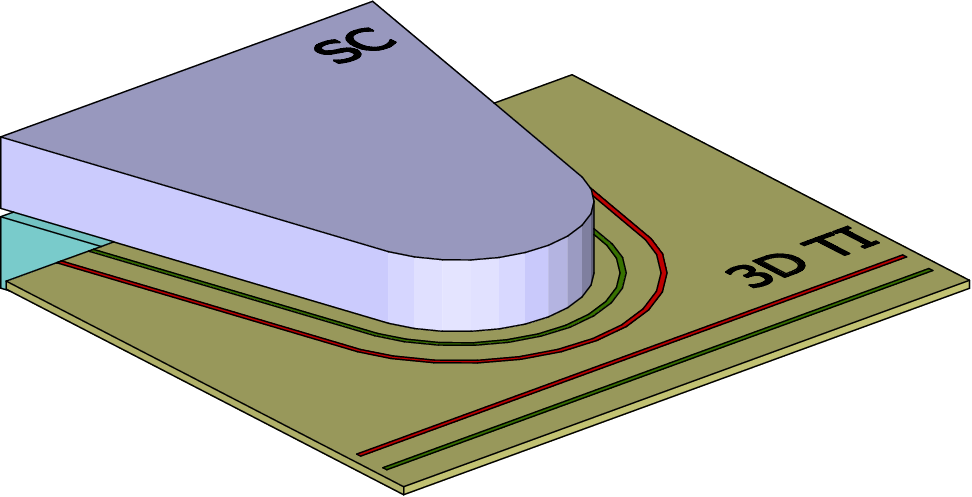
To realize both 1D helical Luttinger liquids as well as 1D helical Majorana modes, we adapt a proposal of Ref. [22] based on thin films of 3D topological insulators (3DTI) such as $\text{Bi}_{2}\text{Se}_{3}$ or $\text{Bi}_{2}\text{Te}_{3}$, see Fig. 1. Helical Dirac fermions emerge at the sample edges due to the mixing of the top and bottom surface bands of the thin film.[42, 43] Moreover, helical Majorana modes can be realized by sandwiching the thin film between conventional $s$-wave superconductors. For opposite signs of the superconductor pairing functions on the top and bottom layer, and sufficiently strong proximity-induced pairing amplitude (greater than the mixing gap of the two surfaces), helical Majorana modes are indeed formed as the edge states of the thin film.[22]

In contrast to the converter between helical Dirac fermions and Majorana modes proposed in Refs. [22, 23], we study the charge transport through tunneling junction(s) between a helical Luttinger liquid and helical Majorana modes connected to ground. For systems with broken time-reversal symmetry, where the helical edge states are replaced by chiral ones, such transport phenomena were studied with noninteracting leads[30] and interacting leads.[28] The schematic diagram for single tunneling junction is depicted in Fig. 2, where the voltage difference between the two leads is controlled by the chemical potential $\mu$ imposed on the helical Luttinger liquid lead. The tunneling amplitude $\bar{t}$ is controlled by the width of the junction and is related to the wavefunction overlap between the two leads.

In the real experiments it may not be easy to fix the relative phases of two adjacent superconductors nor fine tune the chemical potential to the topological regimes. For the heterostructure setup we can make the helical Majorana modes by different types of realizations[32], or change the helical modes to time reversal preserved double Majorana end states[31]. The results for tunnel transport to double Majorana end states is the limiting case of helical Majora mode with energy level separations going to infinity, as is shown in Fig. 5.

We consider one helical Luttinger liquid lead and one helical Majorana fermion lead. The Hamiltonian describing this system is $H=H_{L}+H_{M_{0}}+\sum_{\alpha}H_{T_{\alpha}}+\delta H$. The Hamiltonian $H_{L}=\int_{-\infty}^{\infty}dx\mathcal{H}_{L}$ for the helical fermions is a Luttinger liquid Hamiltonian density,

The Hamiltonian for the grounded propagating Majorana fermions on a ring of circumference $L$ is

Here $v_{M,\sigma}=\text{sgn}(\sigma)v_{M}$. The single particle tunneling term between the helical Luttinger liquid lead and helical Majorana fermion lead is described by[30]

Here, $t_{r\sigma\alpha}$ is the tunneling strength, and $\xi_{r\sigma\alpha}$ are complex numbers with $|\xi_{r\sigma\alpha}|=1$. $r$ indicates the left/right movers in $H_{L}$, $\sigma$ denotes the spin index of the Majorana fermions, and $\alpha=1,..,N$ is the number of tunneling channels (junctions) and $x_{\alpha}/y_{\alpha}$ are their spatial coordinates in Luttinger/Majorana leads. We restrict our discussions to $N=1$ and $N=2$ in this paper but the extension to arbitrary $N$ is straightforward and similar to the $N=2$ case. The $N=2$ case is illustrated in Fig. 3.

The remaining $\delta H$ term contains the leading instabilities[27, 28] under the renormalization group analysis in the low-energy sector. We show in the next section why they are not important in our setup. With this simplification the full low-energy effective Hamiltonian becomes $H\simeq H_{L}+H_{M_{0}}+\sum_{\alpha}H_{T_{\alpha}}$, describing the single-particle tunneling between spinful Luttinger liquids and Majorana fermions lead. The tunneling charge current through site $x_{\alpha}$ (in the helical Luttinger liquid coordinate system) is obtained by

The total tunneling current is the coherent sum of the current from all tunneling channels (under the assumption that the separation distance between junctions are less than the coherence length). We choose a time dependent gauge transformation to move the chemical potentials in $H_{L}$ to $H_{T}$ by writing $\psi_{R/L}\rightarrow e^{i\mu t}\psi_{R/L}$. By defining the Keldysh contour ordered Green’s function $G_{\sigma,R/L,\alpha}(t,t^{\prime})=-i\langle T_{c}\{\gamma_{\sigma}(y_{\alpha},t)\psi^{\dagger}_{R/L}(x_{\alpha},t^{\prime})\}\rangle$ we rewrite the particle current as

This lesser mixed Green’s function $G_{\sigma,j,\alpha}^{<}(t,t)$ is obtained by perturbation theory as

In applying the Wick theorem in the Eq.(5) we should also include all possible four fermions interactions term ($u_{2}$ and $u_{4}$ term in the edge states Hamiltonian) between any two fermions operators. We use the spinless bosonization[34] as a way to sum up all orders of perturbations in the four fermions interactions on the Keldysh contour. The edge state correlators evaluated this way is thus fully dressed by the four fermions interactions in our treatment and we do not specify this aspect in the expression of Eq. (5).

We bosonize the helical Luttinger liquids lead operators by writing the fermion fields as:

with $\eta_{R/L}$ as the Klein factor chosen to satisfy the fermion anti-commutation rule and $a_{0}$ as the lattice spacing cutoff for the linear spectrum. We define the bosonic fields $\Phi,\Theta=\phi_{L}\pm\phi_{R}$ and rewrite $H_{0}=H_{L}+H_{M_{0}}$ and $H_{T}$ as

with Luttinger parameter $K=\sqrt{\frac{2\pi v_{F}+u_{4}-u_{2}}{2\pi v_{F}+u_{4}+u_{2}}}$ and velocity $v=v_{F}\sqrt{(1+\frac{u_{4}}{2\pi v_{F}})^{2}-(\frac{u_{2}}{2\pi v_{F}})^{2}}$. Eq. (7) serves as the main Hamiltonian for computing the tunneling current in section IV. For a single tunneling point contact with time reversal symmetry preserved we set $t_{R\uparrow\alpha}=t_{L\downarrow\alpha}=\bar{t}_{\alpha}$ and otherwise zero. We discuss why other relevant perturbations $\delta H$ are not important in this time reversal preserved system in the next section.

We start with single point contact between the helical Luttinger liquid and helical Majorana modes realized in a time-reversal symmetric topological superconductor. From Ref. 36 the Keldysh component of bare (uncoupled) lead Green functions, defined as $G_{\psi_{L/R}}(\tau,\tau^{\prime})=-i\langle T_{c}\{\psi_{L/R}(\tau)\psi_{L/R}^{\dagger}(\tau^{\prime})e^{-i\mu_{L/R}(\tau^{\prime}-\tau)}\}\rangle$, expressed in frequency space at zero temperature are[37]

Here $\kappa=\frac{1}{4}(K+1/K)$ and $\tilde{h}(\kappa)=2e^{-\pi i\kappa}\sin(\pi\kappa)\Gamma(1-\kappa)^{2}$ and plus/minus sign on $G_{\psi_{L/R}}$ indicates its labeling on the Keldysh contour (with $G_{\psi_{L/R}}^{++}$ as time ordered and $G_{\psi_{L/R}}^{--}$ as anti-time ordered). By relabeling the spin index in $\gamma_{\sigma}$ by the left/right-movers label of the Luttinger lead operator, the steady state charge current is expressed as

Here $n$, $m$ denote the discrete energy levels in the finite size helical Majorana modes. Eq.(13) follows from maintaining the structure of first order expansion in Eq.(5) and resum all higher order terms through the ”dressed” helical Majorana Green’s function. The retarded helical Majorana Green’s function contains higher order terms through inclusion of self energy terms:

Here the ”bare” retarded helical Majorana Green’s function is $G_{\gamma_{j,nm}}^{(0)R}(\omega)=\delta_{n,m}/(w-\epsilon_{n,j}+i0^{+})$ with $\epsilon_{n,j}=\hbar v_{M}\text{sgn}(j)\frac{2\pi n}{L}$ (with $\text{sgn}(j)=+/-$ for $L/R$), and the retarded self energy is $\Sigma_{j,nm}^{R}(\omega)\equiv\frac{t_{j,n}t_{j,m}^{\ast}}{2}G_{\psi_{j}}^{R}(\omega)$ given by the Dyson equation. The dressed helical Majorana lesser Green’s function is $G_{\gamma_{j,nm}}^{<}(\omega)=G_{\gamma_{j,nl}}^{R}(\omega)\Sigma_{j,ll^{\prime}}^{<}(\omega)G_{\gamma_{j,l^{\prime}m}}^{A}(\omega)$ with $\Sigma_{j,nm}^{<}(\omega)\equiv\frac{t_{j,n}t_{j,m}^{\ast}}{2}G_{\psi_{j}}^{<}(\omega)$. Similar expressions hold for $G_{\gamma_{j,nm}}^{A}(\omega)$ and $G_{\gamma_{j,nm}}^{>}(\omega)$.

In Eq. (13) the summation over integers $n$, $m$ (and $l$,$l^{\prime}$ in Eq.(14)) refers to the sum over discrete Majorana modes energy level indices. From this the expression for the current is related to the evaluation of $G_{\psi_{j}}^{<}(\omega)=G_{\psi_{j}}^{+-}(\omega)$, $G_{\psi_{j}}^{A}(\omega)=G_{\psi_{j}}^{++}(\omega)-G_{\psi_{j}}^{-+}(\omega)$, and the aforementioned dressed helical Majorana Green’s functions. In this paper we assume the energy difference between different Majorana modes is sufficient large (greater than the broadening effect coming from coupling with the Luttinger lead) such that $\Sigma_{j,nm}(\omega)\simeq\Sigma_{j}(\omega)\delta_{n,m}$ to simplify the calculation. In other words, we consider the helical topological insulator as short, such that the finite size makes the energy difference between discrete Majorana modes sufficient large so that the overlap between them is negligible. Under this assumption the helical Majorana Green’s functions $G_{\gamma_{j,nm}}^{>}(\omega)$ and $G_{\gamma_{j,nm}}^{R}(\omega)$ are diagonal and the analytic expression for Eq. (13) is obtained. From there we evaluate the current numerically and obtain its relation with bias voltage $V=(\mu-0)/e$ to evaluate the differential conductance. The results for single tunneling junction, with different Luttinger parameters $K$ indicating different interaction strengths, are shown in Fig. 4.

In Fig. 4 we see the perfect transmission (maximum differential conductance) at zero voltage for a noninteracting ($K=1$) helical Luttinger liquid. It originates from the perfect Andreev reflection between the metal and superconductor mediated by the helical Majorana modes.[30] The Majorana modes inside the superconducting gap serve as resonance levels which facilitates the Andreev reflection process and give a differential conductance value $g_{1}e^{2}/h$ with $g_{1}=2\times 2=4$, reflecting particle-hole and spin symmetry. This perfect transmission signature is used to identify the Majorana zero modes in the nanowire experiments.[11] The periodic peaks at finite bias voltages, similar to the case of tunneling measurement chiral Majorana modes discussed in Ref. [30], come from discrete Majorana energy levels with energy difference (peak intervals) set by the physical size of the edge of helical topological superconductor. For (repulsive) interacting lead the general feature is the suppression of the resonant conductance peaks, both in peak magnitude and width, and the spreading out of spectral weight away from the resonance levels.[36]

The spreading of spectral weight makes the transition from perfect Andreev reflection to perfect normal reflection more difficult to observe at smaller Luttinger parameter $K$. This is because the Majorana levels begins to merge together (as shown for $K=0.3$ case in the Fig. 4), violating our starting assumption that the levels are sufficient far apart. To illustrate this kind of metallic (perfect Andreev reflection) to insulating (perfect normal reflection) behavior in this single tunneling junction context, we plot the differential conductance for a single level (zero energy) helical Majorana mode in the Fig. 5. We see that the transition takes place between $K=0.3$ and $K=0.2$ with marked tendency differences between the two at finite bias.

The scaling analysis mentioned in the previous section for single Majorana mode gives $D[\bar{t}]=(K+1/K)/4$, resulting in a critical Luttinger parameter $K_{cr}=2-\sqrt{3}$ for the repulsive helical Luttinger lead. This scaling/criticality behavior is the same as the case for two helical Luttinger liquids connected (with particle-hole symmetry imposed, or $\mu_{1}=-\mu_{2}=eV/2$) by a noninteracting single level quantum dot discussed in Ref. [36]. The vanishing charge transport at zero bias below $K=K_{cr}$ corresponds to the transition point where some quantum information stored by qubits formed by Majorana modes is maintained and does not decohere completely.[38] In general, for charge transport we can formally make analogy between the two helical Luttinger leads with particle-hole symmetric driven voltage connected via a noninteracting multi-level quantum dot system with our single helical Luttinger lead connected with the helical Majorana modes.

Note that once introducing time-reversal-invariance breaking terms[28] or different ways[27] of connecting the Majorana modes, the critical behavior in the charge transport could occur at different $K_{cr}$. For example, if we replaced the helical Majorana modes by the chiral Majorana modes (the edge state of a topological superconductor with broken time reversal symmetry),[28] similar metallic to insulating behavior is seen but with scaling behavior controlled by $D[\bar{t}]=1/2K$, or $K_{cr}=1/2$. Thus for single Majorana modes (or other modes sufficiently far apart such that the overlap is not significant) different scaling behaviors in the single tunnel junction transport reveals a great deal of information about the boundary conditions imposed on the Luttinger liquid.

In a real experiment there is a finite length region where tunneling between the Majorana modes and helical lead occurs. Assuming a separable form for the spatial dependence of tunneling term[39, 40] the analytic expressions for weak tunneling current are obtained for the case of leads made of same type of material. For tunneling between helical Luttinger leads, the power-law dependence is modified for an extended contact compared to the case of a point like contact.[40] Extension of this formulation to infinite-size helical Majorana lead case seems to be straightforward but not so easy for the case of a finite helical Majorana lead. Therefore, we proceed with the simpler case: the case of two quantum point contacts.

Proposals for double point contact setups are mainly related to the study of quantum interference effects[44, 45] and the quasi-particles statistics of the edge states.[46, 47, 48] Similar setups for the helical edge states have been discussed[50, 51, 52, 54] with the possible applications for electronic means of spin pumping[53, 55]. Different types of interferometers have also been proposed for heterostructures of topological superconductor and normal metal/edge states of topological insulators such as the Majorana Dirac converter.[22, 23, 49] Here, the double point contact between the helical Luttinger liquid and the Majorana modes is yet another type of heterostructure showing the quantum interference which is analogous to the two point source interference in optics.

For two point contacts the total current passing through those contacts is $\langle\hat{I}\rangle=\langle\hat{I}_{x_{1}}+\hat{I}_{x_{2}}\rangle$. Without loss of generality we choose $x_{1}=0$, $x_{2}=x$, $y_{1}=0$ and $y_{2}=y$. Here $x_{i}$ denotes spatial coordinate of the fermion operators in the helical Luttinger lead and $y_{i}$ denotes that of the helical Majorana operators in the topological superconductor. We evaluate the current $\langle\hat{I}\rangle$ via perturbations on the tunneling term $H_{T}$ on the Keldysh contour. To simplify the notation we denote $G_{(\psi/\gamma)_{\alpha}}^{(0)}$ as the bare (unperturbed) helical fermion/Majorana mode with chiral (or spin) and position index $\alpha$ and concentrate on the structure of perturbation in the Dyson equation without bookkeeping the Keldysh contour labels on the Green’s functions for the moment. We get:

Note that we do not have spin flip process in the tunneling term, and the $G_{\psi_{\beta}\psi_{\alpha}}$ or $G_{\gamma_{\beta}\gamma_{\alpha}}$ are diagonal in spin space and functions of differences in the spatial coordinate. In these simplified notations the current at position $x_{\alpha}$ of the helical Luttinger lead coordinate is

It is easy to check that above formula gives the single point contact result (13) by taking $t_{\alpha}=\bar{t}/\sqrt{2}$, $t_{\beta}=0$, and with the Langreth theorem[60] (to denote the contour order). Following the same recipes the current for two point contacts with $t_{\alpha}=\bar{t}_{1}/\sqrt{2}$ and $t_{\beta}=\bar{t}_{2}/\sqrt{2}$ is then expressed as:

Here $G_{\gamma_{j}}^{(0)R}(\omega,y)=\sum_{n}\frac{e^{-\text{sgn}(j)i\frac{2\pi n}{L}y}}{\omega-\epsilon_{n,j}+i\eta}$ and $G_{\gamma_{j}}^{(0)<}(\omega,y)=2\pi i\sum_{n}e^{-i\text{sgn}(j)\frac{2\pi n}{L}y}\theta(-\omega)\delta(\epsilon_{n,j}-\omega)$ are the unperturbed retarded and lesser Green’s function for helical Majorana modes, label $j=\pm 1$ denotes left/right moving mode, and $x_{12}=x_{1}-x_{2}$ and $y_{12}=y_{1}-y_{2}$ are the spatial coordinate differences. Following Eqs. (15) and (16) and the Langreth rule we obtain the various dressed Majorana Green’s functions and unperturbed helical fermions Green’s functions needed for evaluating the current. The derivations and analytic expressions for various Green’s functions are shown in the Appendix B and C. With the analytic expressions shown in the Appendices, we perform numerical integrals to compute the current (18) and obtain the differential conductance by taking numerical derivatives with respect to the source drain voltage $V$. The results are shown in the Figs. 6–9.

We chose a small separation length ($x_{12}=y_{12}=10^{-2}L$) between the two contacts in the Fig. 6 and fixed the tunneling strengths of the two point contacts to be identical. The interference effect due to two point contacts for the weakly interacting lead ($K\simeq 1$) is not apparent, and the resonance structure is similar to the single point contact. For a noninteracting lead ($K=1$ or blue solid line in Fig. 6) the differential conductance reaches its maximum value $g_{2}e^{2}/h$ with $g_{2}=2\text{(particle hole)}\times 2\text{(spin)}\times 2\text{(2 tunneling points)}=8$ when the chemical potential of the helical lead is in line with the discrete Majorana energy levels. For a helical lead with stronger repulsion (say $K=0.5$ or purple dashed line in Fig. 6) we see features similar to the single point contact (with shrinking peak width and height at resonance value and transfer of spectral weight away from the resonance) and the effect of interference between two point contacts. Around zero bias the peak splits into two, similar to the physics of Fano resonance, and slight modulations in the resonance positions in other finite voltage peaks. To further study the interference effect we fix $K=0.5$ and plot different separation lengths (still keeping $x_{12}=y_{12}$ and $x_{12}/L\sim 10^{-2}$) in Fig. 7. We see the subpeak structure (see the inset of Fig. 7) also emerges nearby finite voltage resonance peaks with peak heights at a fixed voltage depending on the separation distance. This kind of subpeak structure mainly comes from the change in the real part of self energy correction on the Majorana Green’s function, which emerges with the cancellation of fast oscillating term related to $e^{ik_{F}sgn[j]x_{12}}$ in the $G_{\psi_{\alpha}\psi_{\beta}}$ in the Appendix C from different orientations.

For longer separation distance the interference effect also brings a change in the peak heights. To demonstrate this we choose $x_{12}=y_{12}=0.1L$ in Fig. 8 such that the separation distance is one tenth of the linear dimension of the Majorana modes. Other than the subpeak structure seen for $K=0.5$ case we now also see modulations in the resonance peak heights. This larger envelope (modulation with large voltage range) is associated with the separation length scale being comparable with the Majorana system size. For off resonance region ($K=1$ plot with voltage between $eV/\Lambda=0$ to $0.1$ in Fig. 8, for example) we also see small oscillations around zero which is attributed to the inaccuracy of numerical integrals for fast oscillating functions.

For general double point contacts we could have different tunneling amplitudes $t_{1}$, $t_{2}$ and different separation distances $|x_{12}|\neq|y_{12}|$. For $|t_{1}|\gg|t_{2}|$ or $|t_{1}|\ll|t_{2}|$ the transmitted current is dominated by one of the point contact, and the result is basically the same as that of the single point contact. For $|x_{12}|\neq|y_{12}|$ but with $|t_{1}|=|t_{2}|$ and $|x_{12}|\approx|y_{12}|$ the general features are similar to what we have mentioned in this section. Here we discuss the case of identical separation length $|x_{12}|=|y_{12}|=10a_{0}$ but with different tunneling amplitude $t_{1}=t_{2}e^{i\phi}$. We plot differential conductance around zero bias as a function of the tunneling phase difference $\phi$ for different Luttinger parameters in Fig. 9. For small separation distance chosen here $\phi=\pi$ or $t_{1}=-t_{2}$ leads to almost complete cancellation of the resonance peak. For larger separation distance the general feature is the same (decreasing $dI/dV$ with increasing $\phi$) but with finite conductance even at $\phi=\pi$.

References

- [1] M. Z. Hasan and C. L. Kane, Rev. Mod. Phys. 82, 3045 (2010).
- [2] X. Qi and S.-C. Zhang, Rev. Mod. Phys. 83, 1057 (2011).
- [3] A. M. Essin and V. Gurarie, Phys. Rev. B 84, 125132 (2011).
- [4] R. S. K. Mong and V. Shivamoggi, Phys. Rev. B 83, 125109 (2011).
- [5] B. A. Bernevig, T. L. Hughes, and S.-C. Zhang, Science 314, 1757 (2006).
- [6] C. L. Kane and E. J. Mele, Phys. Rev. Lett. 95 226801 (2005).
- [7] M. König, S. Wiedmann, C. Brüne, A. Roth, H. Buhmann, L. W. Molenkamp, X.-L. Qi and S.-C. Zhang, Science 318, 766 (2007).
- [8] I. Knez, R.-R. Du, and G. Sullivan, Phys. Rev. Lett. 107, 136603 (2011).
- [9] C. W. J. Beenakker, Annu. Rev. Con. Mat. Phys. 4, 113 (2013).
- [10] J. Alicea, Rep. Prog. Phys. 75, 076501 (2012).
- [11] V. Mourik, K. Zuo, S. M. Frolov, S. R. Plissard, E. P. A. M. Bakkers, and L. P. Kouwenhoven, Science 336, 1003 (2012)
- [12] S. Nadj-Perge, I. K. Drozdov, J. Li, H. Chen, S. Jeon, J. Seo, A. H. MacDonald, B. A. Bernevig, and A. Yazdani, Science 346, 602 (2014)
- [13] L. Fu, and C. L. Kane, Phys. Rev. Lett. 100, 096407 (2008).
- [14] X.-L. Qi, T. L. Hughes, S. Raghu, and S.-C. Zhang, Phys. Rev. Lett. 102, 187001 (2009).
- [15] Y. Tanaka, T. Yokoyama, A. V. Balatsky, and N. Nagaosa, Phys. Rev. B 79, 060505 (2009).
- [16] M. Sato and S. Fujimoto, Phys. Rev. B 79, 094504 (2009).
- [17] J. Wang, Y. Xu, and S.-C. Zhang, Phys. Rev. B 90, 054503 (2014).
- [18] R. Queiroz and A. P. Schnyder, Phys. Rev. B 91, 014202 (2015).
- [19] C. Wu, B. A. Bernevig, and S.-C. Zhang, Phys. Rev. Lett. 96, 106401 (2006).
- [20] C. Xu, J. E. Moore, Phys. Rev. B 73, 045322 (2006).
- [21] T. Li, X. Mu, X. Liu, P. Wang, H. Fu, X. Lin, K. Schreiber, G. Csathy, L. Du, G. Sullivan, R.-R. Du, 2015 APS march meeting, unpublished.
- [22] C.-X. Liu and B. Trauzettel, Phys. Rev. B 83, 220510(R) (2011).
- [23] B. Bri, Phys. Rev. B 85, 140501(R) (2012).
- [24] Y. Asano, Y. Tanaka, and N. Nagaosa, Phys. Rev. Lett. 105, 056402 (2010).
- [25] S. Gangadharaiah, B. Braunecker, P. Simon, and D. Loss, Phys. Rev. Lett. 107, 036801 (2011).
- [26] C. P. Orth, R. P. Tiwari, T. Meng, and T. L. Schmidt, arXiv:1405.4353 [cond-mat.mes-hall] (2014)
- [27] L. Fidkowski, J. Alicea, N. H. Lindner, R. M. Lutchyn, and M. P. A. Fisher, Phys. Rev. B 85, 245121 (2012).
- [28] Y.-W. Lee and Y.-L. Lee, Phys. Rev. B 89, 125417 (2014).
- [29] I. Affleck and D. Giuliano, J. Stat. Mech., P06011 (2013).
- [30] K. T. Law, P. A. Lee, and T. K. Ng, Phys. Rev. Lett. 103, 237001 (2009).
- [31] C. L. M. Wong and K. T. Law, Phys. Rev. B 86, 184516 (2012).
- [32] R. Queiroz, A. P. Schnyder, Phys. Rev. B. 91, 014202 (2015).
- [33] J. Li, G. Fleury, and M. Büttiker, Phys. Rev. B 85, 125440 (2012).
- [34] T. Giamarchi, Quantum physics in one dimension, Oxford university press (2004).
- [35] T. L. Schmidt, Phys. Rev. Lett. 107, 096602 (2011).
- [36] S. P. Chao, S. A. Silotri, and C. H. Chung, Phys. Rev. B 88, 085109 (2013).
- [37] Extra factor of in the denominator here comes from different definition of Fourier transform to frequency domain used in Eq.(A9) here and Eq.(A10) in Ref. 36.
- [38] S. H. Ho, S. P. Chao, C. H. Chou, and F. L. Lin, New J. Phys. 16, 113062 (2014).
- [39] D. Chevallier, J. Rech, T. Jonckheere, C. Wahl, and T. Martin, Phys. Rev. B 82, 155318 (2010).
- [40] G. Dolcetto, S. Barbarino, D. Ferraro, N. Magnoli, and M. Sassetti, Phys. Rev. B 85, 195138 (2012).
- [41] Overall magnitude here means we sum the peaks’ magnitude if one peak splits into two due to interference.
- [42] C. X. Liu, H. J. Zhang, B. Yan, X. L. Qi, T. Frauenheim, X. Dai, Z. Fang, and S. C. Zhang, Phys. Rev. B 81, 041307 (2010).
- [43] H. Z. Lu, W. Y. Shan, W. Yao, Q. Niu, and S. Q. Shen, Phys. Rev. B 81, 115407 (2010).
- [44] C. de C. Chamon, D. E. Freed, S. A. Kivelson, S. L. Sondhi, and X. G. Wen, Phys. Rev. B 55, 2331 (1997).
- [45] B. I. Halperin, A. Stern, I. Neder, and B. Rosenow, Phys. Rev. B 83, 155440 (2011).
- [46] D. E. Feldman, Y. Gefen, A. Kitaev, K. T. Law, and A. Stern, Phys. Rev. B 76, 085333 (2007).
- [47] P. Bonderson, K. Shtengel, and J. K. Slingerland, Annals of Physics 323, 2709 (2008).
- [48] P. Bonderson, K. Shtengel, and J. K. Slingerland, Phys. Rev. Lett. 97 016401 (2006).
- [49] A. R. Akhmerov, Johan Nilsson, and C. W. J. Beenakker, Phys. Rev. Lett. 102, 216404 (2009).
- [50] P. Virtanen and P. Recher, Phys. Rev. B 83, 115332 (2011).
- [51] B. Rizzo, L. Arrachea, and M. Moskalets, Phys. Rev. B 88, 155433 (2013).
- [52] C. W. Huang, S. T. Carr, D. Gutman, E. Shimshoni, A. D. Mirlin, Phys. Rev. B 88, 125134 (2013).
- [53] F. Dolcini, Phys. Rev. B 83, 165304 (2011).
- [54] C. P. Orth, G. Strübi, T. L. Schmidt, Phys. Rev. B, 88, 165315 (2013).
- [55] R. Citro, F. Romeo, and N. Andrei, Phys. Rev. B 84, 161301 (2011).
- [56] P. Mehta and N. Andrei, Phys. Rev. Lett. 96, 216802 (2006).
- [57] S. P. Chao and G. Palacios, Phys. Rev. B 83, 195314 (2011).
- [58] M. Abramowitz and I. A. Stegun, Handbook of Mathematical Functions, Applied Mathematics Series, Vol. 55 (National Bureau of Standards, Washington, DC, 1972).
- [59] B. Braunecker, C. Bena, and P. Simon, Phys. Rev. B 85, 035136 (2012).
- [60] H. Haug and A.-P. Jauho, Quantum Kinetics in transport and optics of semiconductors, Springer-Verlag (1998).