The Supersymmetric Standard Model
with Inverse Seesaw at the Large Hadron Collider
S. Khalil1 and S. Moretti2
1 Center for Fundamental Physics, Zewail City for Science and Technology, 6 October City, Cairo, Egypt.
3 School of Physics & Astronomy, University of Southampton, Highfield, Southampton, UK.
Abstract
We review the TeV scale extension of the Minimal Supersymmetric Standard Model (BLSSM) where an Inverse Seesaw mechanism of light neutrino mass generation is naturally implemented and concentrate on its hallmark manifestations at the Large Hadron Collider (LHC).
1 Introduction
The solid experimental evidence for neutrino oscillations, pointing towards non-vanishing neutrino masses, is one of the few firm hints for physics Beyond the Standard Model (BSM). Neutrinos are strictly massless in the SM due to two main reasons: the absence of right-handed neutrinos; the SM has an exact global Baryon minus Lepton number conservation. However, the minimal extension of the SM, based on the gauge group , can account for light neutrino masses through either a Type-I Seesaw or an Inverse Seesaw (IS) mechanism [1, 2]11 1 For old attempts at analysing a high scale extension of the SM, see Ref. [3]..
In the type-I Seesaw mechanism right-handed neutrinos acquire Majorana masses at the symmetry breaking scale, which can be related to the Supersymmetry (SUSY) breaking scale, i.e., TeV, therefore the Yukawa neutrino coupling must be [4]. In contrast, in the IS case, these Majorana masses are not allowed by the gauge symmetry and another pair of SM gauge singlet fermions with tiny masses keV) must be introduced. In this case, there is no severe constraint imposed on the neutrino Yukawa couplings and the possibility of testing this type of model at the LHC is quite feasible. Moreover, in the limit of the above mentioned tiny mass, we have essentially massless light neutrinos. Therefore, such a small scale can be considered as a slight breaking of a global symmetry, hence, according to ’t Hooft criteria, the smallness of this scale becomes natural. One of these two singlet fermions couple to right-handed neutrinos and is involved in generating the light neutrino masses. The other singlet (which is usually called inert or sterile neutrino) is completely decoupled and interacts only through the gauge boson, therefore it may account for warm Dark Matter (DM) [5], see also Refs. [6, 7].
In both scenarios, this model induces several testable signals at the LHC involving the new predicted particles: a (neutral gauge boson associated with the group), an extra Higgs state (an additional singlet state is introduced to break the gauge group spontaneously) and three (Type-I) or six (IS) heavy neutrinos, (that are required to cancel the associated anomaly and are necessary for the consistency of the model). This is the setup for the non-SUSY sector of the scenario, which is well established in the literature (see Refs. [8, 9] for a review of its main phenomenological manifestations).
It is the purpose of this paper to review its Supersymmetric version, the BLSSM, particularly in the IS framework. The reason to concentrate on the IS version of the BLSSM is twofold. On the one hand, its phenomenological exploitation is more recent and less evolved with respect to the type-I Seesaw mechanism case, hence the need of reviewing its status in view of the ongoing Run 2 stage of the LHC. Secondly, the former appears to have some intriguing and testable features in the Higgs sector that the latter has not (as we shall try to emphasise), again, calling for a timely assessment of the LHC sensitivity to it, given the high priority that Higgs physics has for Run 2.
The plan of the paper is as follows. In the next section we proceed to the construction of the BLSSM Lagrangian. In Sect. 3 we describe how dynamical Electro-Weak Symmetry Breaking (EWSB) occurs in the BLSSM whereas in Sect. 4 we introduce its particle spectrum. In Sect. 5 we study in particular the Higgs masses. Then, in Sect. 6, we describe the main manifestations of the BLSSM at the LHC. We conclude in Sect. 7.
2 Constructing the BLSSM
The particle content of this model includes the following superfields in addition to those of the Minimal Supersymmetric Standard Model (MSSM): two SM singlet chiral Higgs superfields , whose Vacuum Expectation Values (VEVs) of their scalar components spontaneously break the and is required to cancel the anomaly; three sets of SM singlet chiral superfields, , to implement the IS mechanism (also in order to cancel the anomaly). Tab. 1 provides the particle content of the SUSY version of the model with IS (henceforth BLSSM-IS for short) as well as the different charge assignments of each Superfield.
| Superfield | Spin 0 | Spin | Generations | |
|---|---|---|---|---|
| 3 | ||||
| 3 | ||||
| 3 | ||||
| 3 | ||||
| 3 | ||||
| 3 | ||||
| 3 | ||||
| 3 | ||||
| 1 | ||||
| 1 | ||||
| 1 | ||||
| 1 |
The superpotential of the leptonic sector in this model is given by [10]
| (1) |
In order to prevent a possible large mass term , we assume that the superfields , and are even under matter parity, while is an odd particle. By assuming a minimal Supergravity (mSugra) inspired universality of parameters at the scale of a Grand Unification Theory (GUT), we obtain that the SUSY soft breaking Lagrangian is given by
where the trilinear terms are defined as .
The symmetry is radiatively broken by the non-vanishing VEVs () while the EW one by the non-zero VEVs , with GeV, TeV and the ratio of these VEVs are defined as and [4]. After and EW symmetry breaking, the neutrino Yukawa interaction terms lead to the following expression:
| (2) |
where and . In this framework, the light neutrino masses are related to a small mass term in the Lagrangian, with KeV, which can be generated at the scale through a non-renormalisable higher order term , where is the mass of a heavy state whose loop(s) or tree-level tadpole diagrams generate the corresponding higher order term ( in our case).Therefore, one finds that the neutrinos mix with the fermionic singlet fields to build up the following mass matrix, in the basis :
The diagonalisation of the mass matrix, Eq. (2), leads to the following light and heavy neutrino masses, respectively:
| (7) | |||||
| (8) |
Thus, one finds that the light neutrino masses can be of order eV, with a TeV scale , if , and a order one Yukawa coupling . Such a large coupling is crucial for testing the BLSSM-IS and probing the heavy neutrinos at the LHC. As shown in [12], the mixings between light and heavy neutrinos are of order . Therefore, the decay widths of these heavy neutrinos into SM fermions are sufficiently large. It is worth mentioning that the second SM singlet fermion, , remains light with mass given by
| (9) |
where is a sort of inert/sterile neutrino that has no mixing with the active neutrinos. It can therefore be a good candidate for warm DM as emphasised in Ref. [5].
3 Radiative symmetry breaking in the BLSSM-IS
The breaking of can spontaneously occur through the VEV of the scalar field or the right-handed sneutrino [4], depending on the initial values of the Yukawa couplings and soft terms involved in the Renormalisation Group Equations (RGEs) of the parameters in the scalar potential , where
| (10) |
where , and is the gauge coupling of . The stablitity condition of is given by
| (11) |
The minimisation of this potential, , implies that
| (12) | |||
| (13) |
where (no mixing between and is assumed here). From (12)–(13), one gets
| (14) |
where . Note that, again from (12)–(13), we also get
| (15) |
Now we complete our analysis of symmetry breaking. We have
| (16) | |||||
| (17) | |||||
| (18) |
where . To show that the symmetry will be broken spontaneously, we must ensure that the point is not a local minimum of the potential . Since and we should impose a condition to make a saddle point. This condition is
| (19) |
It is worth noting that it is impossible to simultaneously fulfil both the conditions (11) and (19) for positive values of and . However, one should note that the condition (19) is valid at the symmetry breaking scale, where the running of the RGEs, from the GUT scale down to the breaking scale, may induce negative squared mass of . At this scale both conditions (11) and (19) are satisfied and symmetry is spontaneously broken with stable potential. This can be seen as follows.
The RGEs for are given by
| (20) | |||||
| (21) |
where and is the gaugino mass of , which is given by at the GUT scale, . In order to solve these equations, we should take into account all involved RGEs, given in Ref. [11]. Fig. 1 reports the result of the running. In plotting this figure, we set the following mSugra inspired conditions at the high scale, e.g., GeV and an order one ratio . As can be seen from the plot, drops rapidly to a negative mass region whereas remains positive. Also in Fig. 1, we plot the scale evolution for the scalar mass as well as for and . The figure illustrates that they remain positive at the TeV scale. Therefore, the breaking via a non-vanishing VEV for right-handed sneutrinos does not occur in the present framework.
Before closing this section, let us emphasise that in the BLSSM with Type I Seesaw the symmetry is spontaneously broken by the VEV of scalar singlet only if the Yukawa coupling of the term is assumed to be degenerate, i.e. . If one assumes a hierarchical texture, where for instance only gives important contributions, one finds that right-handed sneutrino may acquire a VEV before and breaks both and -parity. However, here, within the BLSSM-IS, the situation is different. One can show that, even with one non-vanishing Yukawa, will acquire a VEV before the right-handed sneutrino such that is spontaneously broken while -parity remain conserved [13].
4 The BLSSM-IS Spectrum
We have seen the evolution of different parameters from the GUT to the scale. Once the symmetry is broken and so is the EW one too (at the scale), different particles with different quantum numbers can mix and acquire new mass eigenstates. Here, we will focus on the new particles associated with the symmetry, namely, the gauge boson, extra Higgs bosons and right-handed sneutrinos. We shall do so in three separate subsections.
Before proceeding to doing so, we should mention that, in all the analyses below, we have used the SARAH [14] and SPheno [15, 16] to build the BLSSM. Furthermore, the matrix-element calculation and event generation were derived from MadGraph 5 [17] and manipulated with MadAnalysis 5 [18]. Finally, notice that all current experimental constraints, from both collider (LEP2, Tevatron and LHC) and flavour (BaBar, Belle and LHCb) are taken into account in our numerical scans. Also DM and neutrino mass and coupling constraints are enforced throughout.
4.1 The Gauge Boson in the BLSSM-IS
The and gauge kinetic mixing can be absorbed in the covariant derivative redefinition, where the gauge coupling matrix will be transformed as follows:
where
| (27) | |||||
| (28) | |||||
| (29) |
In this basis, one finds
| (30) |
Furthermore, the mixing angle between and is given by
| (31) |
4.2 The Higgs Bosons in the BLSSM-IS
The gauge kinetic term induces mixing at tree level between the and states in the BLSSM scalar potential. Therefore, the minimisation conditions of this potential at tree level lead to the following relations [19]:
| (32) | |||||
| (33) | |||||
where and . Note that, with non-vanishing , the parameter depends on and the sign of . We may have both constructive and destructive interference between the first term and other terms in Eq. (32). In general, we find that the typical value of is of order TeV.
To obtain the masses of the physical neutral Higgs bosons, one makes the usual redefinition of the Higgs fields, i.e.,
and
.
The real parts correspond to the CP-even Higgs bosons and the imaginary parts correspond to the CP-odd Higgs bosons. The squared-mass matrix of the BLSSM CP-odd neutral Higgs fields at tree level, in the basis , is given by
| (34) |
It is clear that the MSSM-like CP-odd Higgs is decoupled from the BLSSM-like one (at tree level). However, due to the dependence of on , one may find TeV).
The squared-mass matrix of the BLSSM CP-even neutral Higgs fields at tree level, in the basis , is given by
| (35) |
where is the usual MSSM neutral CP-even Higgs mass matrix, which leads to the SM-like Higgs boson with mass, at one loop level, of order 125 GeV and a heavy Higgs boson with mass TeV).
In this case, the BLSSM matrix is given by
where and . Therefore, the eigenvalues of this mass matrix are given by
| (40) |
If , one finds that the lightest neutral Higgs state is given by
| (41) |
The mixing matrix is proportional to and can be written as [19]
For a gauge coupling , these off-diagonal terms are about one order of magnitude smaller than the diagonal ones. However, they are still crucial for generating interaction vertices between the genuine BLSSM Higgs bosons and the MSSM-like Higgs states. Note that the mixing gauge coupling constant, , is a free parameter that can be positive or negative [19].
In Fig. 2, we show the masses of the four CP-even Higgs bosons in the BLSSM for and . In this plot we fix the lightest MSSM Higgs boson mass to be of order 125 GeV. As can be seen from this figure, as intimated, one of the BLSSM Higgs bosons, , can be the second lightest Higgs boson ( GeV). Both and are instead quite heavy (since both and are of order TeV).
This sets the stage for the hypothesis made in Ref. [20] (see also [21]), wherein, motivated by a excess recorded by the ATLAS and CMS experiments at the LHC around a mass of order GeV in (CMS) and (both) samples [22, 23, 24, 25], is was shown that a double Higgs peak structure can be generated in the BLSSM, with CP-even Higgs boson masses at and GeV, a possibility instead precluded to the MSSM.
Before proceeding in this respect, though, two remarks are in order: firstly, if , the coupling of the BLSSM lightest Higgs state, , with the SM particles will be significantly suppressed ( relative to the SM strength), so that, in order to account for possible signals at the LHC, this parameter ought to be sizable; secondly, in both cases of vanishing and non-vanishing , one may fine-tune the parameters and get a light , which leads to a MSSM-like CP-even Higgs state, , with GeV. However, it is well known that in the MSSM the coupling is suppressed with respect to the corresponding one of the SM-like Higgs particle by one order of magnitude due to the smallness of , where . In addition, the total decay width of is larger than the total decay width of the SM-like Higgs, , by at least one order of magnitude, because it is proportional to , which is essentially the square of the coupling of to the bottom quark. Therefore, the MSSM-like heavy Higgs signal has a very suppressed cross section and thus cannot be a candidate for light Higgs signals at the LHC.
In the light of this, we will focus in the next section on the lightest BLSSM CP-even Higgs, , as a possible candidate for the second Higgs peak seen by CMS in both and , see Refs. [24, 25]. However, before doing so, we ought to setup appropriately the BLSSM parameter space, in order to find such a solution. As mentioned above, the recent results from CMS indicate a hint of a second Higgs boson at GeV. Herein, for definiteness, we consider GeV as reference BLSSM point.
As emphasised above, in the BLSSM, it is quite natural to have two light CP-even Higgs bosons, and , with mass GeV and GeV, respectively. The CP-even neutral Higgs mass matrix in Eq. (35) can be diagonalised by a unitary transformation:
| (46) |
The mixing elements and are proportional to and they identically vanish if , as one can see in Fig. 3. Also, in this limit, and approach and , respectively, where is the usual CP-even Higgs mixing angle in the MSSM.
The lightest eigenstate is the SM-like Higgs boson, for which we will fix its mass to be exactly 125 GeV. As mentioned, numerical scans of the BLSSM parameter space confirm that the state can then be the second light Higgs boson with mass of (137 GeV). The other two CP-even states, and , are heavy (of TeV). The can be written in terms of gauge eigenstates as
| (47) |
Thus, the couplings of the with up- and down-quarks are given in terms of the elements of the mixing matrix by
| (48) |
Similarly, one can derive the couplings with the and gauge boson pairs:
Since , the coupling of the with , , will be as follows:
| (49) |
where .
4.3 Sneutrino Masses in the BLSSM-IS
Now we turn to the sneutrino mass matrix. If we write and as and , then we get the following mass matrix for the CP-odd sneutrinos:
| (50) |
where , , , and are given in Ref. [10] and are proportional to , , , , and , respectively. The mass matrix for the CP-even sneutrino () is obtained by changing . The sneutrino mass eigenstates can be obtained by diagonalising the mass matrices as
| (51) |
However, the diagonalisation of these matrices is not an easy task and can only be performed numerically. It turns out that the mass of the lightest CP-odd sneutrino, , is almost equal to the mass of the lightest CP-even sneutrino, . Both are generated from the mixing between and . The mass of these lightest sneutrinos can be in the range 400–1400 GeV, as shown in Fig. 4.

5 (S)Neutrino Corrections to the Lightest Higgs Boson Mass
In this section, we calculate the one-loop radiative corrections due to right-handed (s)neutrinos to the mass of the lightest Higgs boson when the latter is SM-like. We show that such effects is in the range GeV, thereby giving an absolute upper limit on such a mass around 170 GeV [10]. The importance of this result from a phenomenological point of view resides in the fact that this enhancement greatly reconciles theory and experiment, by alleviating the so-called ‘little hierarchy problem’ of the minimal SUSY realisation, whereby the currently measured mass of the SM-like Higgs mass is very near its absolute upper limit predicted theoretically, of 130 GeV.
It is important to note that, unlike the squark sector, where only the third generation (stops) has a large Yukawa coupling with the Higgs boson, hence giving the relevant correction to the Higgs mass, all three generations of the (s)neutrino sector may lead to important effects since the neutrino Yukawa couplings are generally not hierarchical. Also, due to the large mixing between the right-handed neutrinos and [26], all the right-handed sneutrinos are coupled to the Higgs boson , hence they can give significant contribution to the Higgs mass correction. In this respect, it is useful to note that the stop effect is due to the running of 12 degrees of freedom (3 colors times 2 charges times 2 for left and right stops) in the Higgs mass loop corrections, just like in the case of right-handed sneutrinos for which there are also 12 degrees of freedom (3 generations times 4 eigenvalues).
To calculate the (s)neutrino corrections to the lightest Higgs mass, we computed, in a previous section, the explicit form of the sneutrino masses, while for the neutrino mass expressions, which are well known, we refer the reader to [10]. Due to one generation of neutrinos and sneutrinos, the one-loop radiative correction to the effective potential is given by the relation
| (52) |
The first sum runs over the sneutrino mass eigenvalues, while the second sum runs over the neutrino masses (with vanishing ). In case of degenerate diagonal Yukawa couplings, one finds that the total is given by three times the value of for one generation. This factor then compensates the colour factor of (s)top contributions.
Therefore, the genuine correction to the CP-even Higgs mass matrix, due to the (s)neutrinos, at the scale at which , is given by
| (53) |
It follows that (see [10] for details)
| (54) | |||||
That is, we have
| (55) | |||||
| (56) |
Therefore, the complete one-loop squared-mass matrix of CP-even Higgs bosons will be given by , with
where refers to the (s)top contribution presented in Eq. (1) of [10] and is the (s)neutrino correction given in Eq. (56). In this case, the lightest Higgs bosons mass is given by
| (60) |
For and , one finds that
| (61) |
If TeV, and GeV, one gets that , thus the Higgs mass is of order GeV GeV.

In Fig. 5 we present the Higgs mass, , as a function of the sneutrino mass, , for GeV and couplings varying from 0.1 to 0.4. As can be seen, in our model the Higgs mass can be easily within the experimental limits. In particular, we have employed the Higgs mass bound as [27, 28], where we take into account about 2 GeV uncertainty in the Higgs boson mass due to the theoretical uncertainties in the calculation of the minimum of the scalar potential, and the experimental uncertainties in and . Finally, notice that all the data points collected satisfy the requirement of radiative EWSB.
6 LHC Signatures of the BLSSM-IS
6.1 Search for the BLSSM-IS
Now we study the signatures of the extra neutral gauge boson in the BLSSM-IS at the CERN machine22 2 In fact, we assume here that all SUSY particles (including sneutrinos) are large enough so that the cannot decay into these, thereby implying that our analysis can be applied also to the standard scenario. We will look at some SUSY effects later on in this review.. The possibility of a decay into a pair of heavy (inert) neutrinos would increase the total decay width of the . Therefore, the Branching Ratio (BR) of (), the prime signal at the LHC, is suppressed with respect to the prediction of, e.g., the Sequential Standard Model (SSM), which is usually considered as benchmark in experimental searches for a . Fig. 6 shows the BRs of all decays. Note that we have assumed that the sfermion are quite heavy so that the decay is dominated by SM particles and light inert/sterile neutrinos.
According to this plot, the BRs of the non-SUSY decays are given by [29]
| (62) |
where , , and refer to the charged leptons, the six quarks, and the six heavy neutrinos respectively. Whereas stands for the three inert neutrinos. In this example we have assumed TeV, , and heavy neutrino masses are set at , and GeV, respectively.
It is worth noting that, in our model, the cross sections (’s) that were used to derive the ATLAS and CMS current mass limit could be simply rescaled by a factor of . If and BR, this reproduces the SSM cross sections that were used by ATLAS and CMS. Considering the scaling of cross sections, the current mass limits will be lowered by a factor of . This result is consistent with the conclusion of Ref. [30].
If GeV were considered, BR could be achieved (e.g., through onsetting decays into inert/sterile neutrinos), in which case fb when and fb when , while in the SSM the BR giving fb for both electron and muon channels. In this respect, the experimental limit TeV by ATLAS [31] ( TeV [32] by CMS) will be lowered, because of a rescaling of the cross section when, e.g., . This yields a new limit of 1.9[0.7] TeV (2.2[0.81] TeV). For reference, Tab. 2 gives () for the SSM and BLSSM-IS at different values.
| [GeV] | [fb] | [fb] (with IS) | ||
|---|---|---|---|---|
| 1000 | 170 | 6 | 41 | 105.7 |
| 1500 | 21.7 | 0.58 | 4.5 | 13.2 |
| 2000 | 3.4 | 0.087 | 0.72 | 2.3 |
| 2500 | 0.8 | 0.015 | 0.15 | 0.58 |
| 3000 | 0.21 | 0.003 | 0.04 | 0.19 |
| 3500 | 0.06 | 0.009 | 0.06 | |
Detecting a signals for such small masses, of order 1 TeV, obtainable for , would only be circumstantial evidence for the BLSSM-IS though, as other models may well feature a similar mass spectrum. A truly smoking-gun signature of the BLSSM-IS would be to produce a and heavy neutrinos simultaneously. Indeed, it turns out that the dominant production mode for heavy neutrinos at the LHC would be through the Drell-Yan (DY) mechanism itself, mediated by the . The mixing between light and heavy neutrinos generates new couplings between the heavy neutrinos, the weak gauge bosons and the associate leptons. These couplings are crucial for the decay of the heavy neutrinos. The main decay channel is through a gauge boson, which may decay leptonically or hadronically. We sketch this production and decay channel via the Feynman diagram given in Fig. 7. Unfortunately, the very fact that ought to be small to comply with current LHC data which rule out detection in the DY induced di-lepton channel for (1 TeV) masses in turn means that such decays also remains unaccessible. One needs a stronger coupling to access the latter, which thus requires higher masses. Hence, for the remainder of this studies, we will adopt a BLSSM-IS benchmark wherein TeV.
Once such a state is produced and decays into , one has to further sample decays. In case of a multi-lepton final state, one ends up with four leptons plus missing energy (), while in case of a multi-hadronic final state states one ends up with four jets plus two leptons (). In addition, it is also possible to have a mixed final state (). (Notice that one or more neutrinos would appear in the detector as missing transverse energy/momentum, .) If two flavours of the heavy neutrinos are assumed to be degenerate in mass, one gets the same final states for the produced heavy neutrino pair with similar event rates. This will double the number of final state events but will make it difficult to distinguish between final state leptons. Therefore, throughout the current study, we consider non-degenerate heavy neutrino masses also including the interference between every two different flavours. (See Refs. [33, 34, 35, 36, 37, 38] for alternative phenomenological analyses in the case of the standard model.)
We thus focus on the possibilities of the LHC in accessing decays into heavy neutrinos in the BLSSM-IS. In doing so, we have carried out full Monte Carlo (MC) event generation using PYTHIA [39] to simulate the initial and final state radiation, fragmentation and hadronisation effects. For detector effects we have used Delphes [40].
We consider the following benchmark: TeV, GeV, GeV and GeV. Of the three decay signatures of the pair discussed in Ref. [29], i.e., , and (), only the latter appeared promising, hence we only focus here on this case, by highlighting the main results33 3 A publication with full details and additional results is in progress [41].. In doing so, we produce our results at TeV assuming a variable luminosity, ranging from the standard 300 fb-1 to the tenfold increase forseen at the Super-LHC [42]. The selections assumed in our analysis are as follows [29]: a transverse momentum, , cut of GeV and a pseudo-rapidity, , cut of 2 were set on each electron while the separation between two electrons, , was enforced to be 0.2. We have assumed no restrictions on , generated for this signature by two neutrinos escaping detection.
The key advantage of this channel is that it is almost background free. The main SM noise comes from (three gauge boson) production with fb at 14 TeV [43, 44]. In Fig. 8 we show the invariant mass of the ‘4 lepton’ system from the signal versus the background and also the transverse mass of the ‘4 lepton + ’ system, where such a variable is defined as
| (63) |
These figures indicate that the decay channel ‘4 lepton + ’ yields a quite clean signature and is rather promising for probing both and after by the end of the standard luminosity run of the LHC by using only few simple cuts to extract the Signal () from the Background (). This is clear from the achievable numbers of events left after the set of cuts mentioned above, alongside their statistical significance, , as a function of the luminosity, see Fig. 9.
One thing should however be noted at this stage, concerning the statistical analysis presented in Fig. 9. Herein, we have at times (i.e., depending on the luminosity) calculated significances using the expression even for event numbers of , which may not be entirely appropriate, as such an approach normally requires large event samples and . In essence, the method is not accurate as it is based on a distribution of test statistics which assumes that noise is negligible. Thus, as an alternative approach, we have used the ‘frequentest method’ too, based on Ref. [45]. With reference to Sect. 2 therein, using our MC samples, we have calculated the expected significance at to reject the null, i.e., background only, hypothesis. For simplicity, we have used only the statistical error for the nuisance parameters, which can easily be extracted from our histograms. Also, we have computed the expected significance in the signal region before and after a somewhat looser final mass cut, in order to allow for a quantitatively sounder comparison (e.g., in the case of TeV only, as the pattern emerging from the selection is similar)44 4 Note that the concept of signal region is obvious where the null hypothesis has to be rejected in the region where the signal is bumped over the background and be accepted in the control region where the sample is background dominated.. From the plots in Fig. 10, it is clear that, at low luminosity, the difference between the frequentist and methods is large while at higher luminosity they tend to converge, with the latter approach overestimating the significance over the former. Clearly, an appropriate merging of the two approaches is eventually required in order to assess the feasibility of our studies at the experimental level, depending on the actual size of the data samples. In fact, to do any cut optimisation is out of scope of this paper, as in real experimental analyses this is actually done using Multi-Variate Analysis (MVA) techniques, which essentially assume a set of chosen cuts for a range of values of each of these then calculate the efficiency for each combination. Then various numerical algorithms are used to decide on the best choice of combination to finally apply in the analysis. What we did here was instead to first characterise the signal and background based on MC truth and then decide the relevant cuts after plotting both of these, which we have done essentially by chosing visually the region where the former exceeds the latter. As we are unable to access such MVA tools, which belong to the repositories of the collaborations, we cannot credibly improve our analysis any further at this stage.
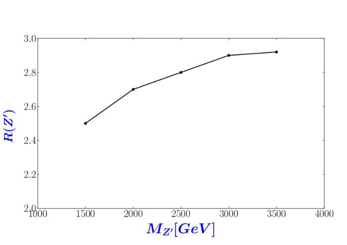
Before closing this section, we should however comment on the influence of the SUSY spectrum on the scope of the signal within the BLSSM. Clearly, once the assumption made so far (that all sparticles are heavier than the ) is dismissed, the boson can decay via SUSY objects. This will correspond to an increased value of its total width , which would then reflect onto the event rates of such a signal. In fact, the latter will scale as the inverse of . In order to quantify this (reduction) effect induced by a low mass spectrum within the BLSSM, we have revisited the benchmarks introduced in Tab. 2, excluding only the 1 TeV mass point (now ruled out by data, as discussed) and thus including the 2.5 TeV benchmark considered so far in our MC analysis. For each of these scenarios we have computed the ratio
| (64) |
the inverse of which corresponds to the rescaling factor to be applied to our event rates for the signal in presence of a low-lying SUSY spectrum in the BLSSM. We can see from Fig. 11 that , obtained from the average total width after scanning the entire BLSSM parameter space compatible with current experimental and theoretical constraints, is typically smaller than 3, so that the rates will generally not be smaller than a factor 1/3 with respect to the values considered here. In fact, also recall that we have not allowed for decays into muons (), which would contribute a factor of towards the signal rates in the ‘4 lepton + ’ channel. The SM rates presented here would of course be unchanged. One should however include intrinsic SUSY backgrounds in the full analysis, as is presently being done in [41]. We can anticipate that the latter would not spoil the feasibility of such a signal as potentially (i.e., modulus experimental verification, both kinematical and statistical) established here over a sizable portion of the full BLSSM parameter space.
6.2 Search for an Extra BLSSM-IS Higgs Boson
The Higgs decay into is one of the golden channels, with low background, to search for Higgs boson(s). The search is performed by looking for resonant peaks in the spectrum, i.e., the invariant mass of the system. In CMS [24], this decay channel shows two significant peaks at 125 GeV and around/above GeV. We define by the total production cross section, dominated by gluon-gluon fusion, computed for GeV, for definiteness. (See Tab. I in [20] for the BLSSM parameters corresponding to this specific benchmark point, which is well compliant with current experimental limits.) From Sect. 4, it is then clear that
| (65) |
(wherein the label SM identifies the SM Higgs rates computed for a 125 GeV mass), which, for GeV, is of order . Also the ratio between BRs can be estimated as
| (66) |
where
| (67) |

First we analyse the kinematic search for the BLSSM-IS Higgs boson, , in the decay channel to . In Fig. 12, we show the invariant mass of the 4-lepton final state from at TeV, after applying a cut of 5[2.5] GeV on each of the four leptons [20]55 5 Transverse momentum and pseudo-rapidity thresholds are slightly different for electrons and muons, but accounting for this subtlety would not change our conclusions.. The SM model backgrounds from the and 125 GeV Higgs boson decays, and , respectively, are taken into account, as demonstrated by the first two peaks in the plot (with the same requirement). It is clear that the third peak at GeV, produced by the decay of the BLSSM-IS Higgs boson into , can reasonably well account for the events observed by CMS [24] with the 8 TeV data. This is shown in Tab. 3, where the mass interval in m4l that we have investigated to extract the signal is wide enough to also capture another prominent 145 GeV anomaly seen in the same CMS data set. (The bin width used in [24] is 3 GeV so potentially able to separate the two peaks at 137 and 145 GeV, yet combining the handful of events under the two peaks makes statistical sense given, on the one hand, the small mass difference and, on the other hand, the fact that for masses so close to the threshold one can find intrinsic BLSSM Higgs widths of order GeV.)
| Number of events for at TeV | ||||
| Higgs mass | Observed | Expected | Background | |
| (CMS) | (BLSSM) | |||
| 125 GeV | 25 | 18.5 | 6.6 | - |
| 136.5 GeV | 29 | 10.2 | 9.15 | 0.8 |
Next we turn to the di-photon channel, which provides the greatest sensitivity for Higgs boson discovery in the intermediate mass range (i.e., for Higgs masses below )66 6 The effects of light SUSY particles leading to a possible enhancement of the di-photon signal strength of the SM-like Higgs boson were studied in [46].. Like the SM-like Higgs, the decays into two photons through a triangle-loop diagram dominated by (primarily) and (in part) top quark exchanges. As shown in Sect. 4, the couplings of the with top quarks and gauge bosons are proportional to some combinations of and , which may then lead to some suppression or enhancement in the partial width . In the SM, . Similarly, in the BLSSM, we have found that, for our GeV benchmark, the BR of in photons amounts to , hence within current experimental constraints.

| Number of events for at TeV | ||
| Higgs mass | Observed (CMS) | Expected (BLSSM) |
| GeV | 610 | 666 |
| GeV | 170 | 177 |
The distribution of the di-photon invariant mass is presented in Fig. 13 for a centre-of-mass energy TeV [20]. Again, here, the observed SM-like signal around 125 GeV is taken as background while the background can now be ignored [47]. As expected, the sensitivity to the Higgs boson is severely reduced with respect to the presence of the already observed Higgs boson, yet a peak is clearly seen at 136.5 GeV and is very compatible with the excess seen by CMS [25]. This is shown in Tab. 4. In fact, ATLAS results point in the same direction as well [22, 23], see [48] and references therein. For example, in [22], they have a slightly worse resolution, of 2 GeV, and use a mixed sample of 7 TeV (with 4.8 fb-1) and 8 TeV (20.7 fb-1) data. If we integrate five bins around 125(137) GeV, see Fig. 3 of [22], we obtain approximately 700(145) events above the background. It is worth mentioning that here we consider both the gluon-gluon fusion and vector-boson fusion modes for both and production.
Before closing this section, we should also mention that the enhancement found in the BLSSM-IS may be mirrored in the decay channel [21] for which, at present, there exists some constraints, albeit not as severe as in the case. We can anticipate (see [21]) that the BLSSM-IS regions of parameter space studied here are consistent with all available data.
7 Conclusions
In summary, in this mini-review, we have introduced the reader to the minimal SUSY version of the well established model with an IS mechanism, that we have termed as BLSSM-IS. This scenario nicely combines the theoretically appealing features of SUSY with key experimental evidence of Beyond the SM (BSM) physics in the form of neutrino masses.
Initially, we have proceeded with the construction of the BLSSM-IS Lagrangian, followed by an illustration of how dynamical EWSB naturally occurs via RGE evolution starting from an mSugra inspired model configuration at high scales. Then, we have described the emerging particle spectrum, by singling out the dynamics in the three specifically BLSSM-IS sectors: i.e., the , Higgs and (s)neutrino parts. In three separate subsections we have in fact derived the relevant masses and couplings.
As EWSB and breaking both occur close to the SUSY mass scale of order 1 TeV, the BLSSM-IS also bears interesting phenomenological manifestations at the LHC in the three aforementioned sectors. Therefore, we have studied next the hallmark signals of this scenario in turn. Firstly, we described production and decay into a variety of leptonic and hadronic signatures proceding via heavy neutrinos77 7 The case of sneutrino mediated channels has been tackled in Ref. [49]., all leading to detectable signals at Run 2 of the CERN machine. Secondly, we highlighted the striking feature of the BLSSM-IS in the Higgs sector, in the form of a possible additional light Higgs resonance yielding sizable and decays which may even explain some anomalies around a mass of 137 to 145 GeV present already in the ATLAS and CMS data of Run 1 of the LHC and which have not yet been ruled out by current Run 2 samples (neither [50] nor [51] ones).
In short, the BLSSM-IS represents a viable realisation of SUSY, compliant with all current data and giving distinctive signatures at the LHC which will enable one to disentangle it from alternative BSM scenarios. These include the simultaneous production of a and heavy (s)neutrinos. Further, these can possibly be accompanied by a second light CP-even Higgs boson signal (precluded to the MSSM), but not by a 750 GeV one [52, 53], as the BLSSM-IS specific CP-even Higgs state is heavier than its MSSM counterpart (see [54] for very recent results in this respect).
Acknowledgements
The work of SK is partially supported by the ICTP grant AC-80. SM is supported in part through the NExT Institute. The work of SK and SM is also funded through the grant H2020-MSCA-RISE-2014 no. 645722 (NonMinimalHiggs). We thank Ahmed Hammad and Juri Fiaschi for assistance in preparing this manuscript.
References
- [1] S. Khalil, J. Phys. G 35, 055001 (2008).
- [2] S. Khalil, Phys. Rev. D 82, 077702 (2010).
- [3] R. N. Mohapatra and R. E. Marshak, Phys. Rev. Lett. 44, 1316 (1980) [Erratum-ibid. 44, 1643 (1980)]; C. Wetterich, Nucl. Phys. B 187, 343 (1981); W. Buchmuller, C. Greub and P. Minkowski, Phys. Lett. B 267, 395 (1991); W. Buchmuller and T. Yanagida, Phys. Lett. B 302, 240 (1993).
- [4] S. Khalil and A. Masiero, Phys. Lett. B 665, 374 (2008); P. Fileviez Perez and S. Spinner, Phys. Rev. D 83, 035004 (2011); T. Kikuchi and T. Kubo, Phys. Lett. B 666, 262 (2008); R. M. Fonseca, M. Malinsky, W. Porod and F. Staub, Nucl. Phys. B 854, 28 (2012).
- [5] A. El-Zant, S. Khalil and A. Sil, Phys. Rev. D 91, 035030 (2015).
- [6] L. Basso, B. O’Leary, W. Porod and F. Staub, JHEP 1209, 054 (2012).
- [7] S. Khalil, O. Seto, JCAP 0810, 024 (2008).
- [8] S. Khalil and S. Moretti, J. Mod. Phys. 4, 7 (2013).
- [9] S. Khalil and S. Moretti, Front. Phys. 1, 10 (2013).
- [10] A. Elsayed, S. Khalil and S. Moretti, Phys. Lett. B 715, 208 (2012).
- [11] F. Staub, Comput. Phys. Commun. 185, 1773 (2014).
- [12] W. Abdallah, A. Awad, S. Khalil and H. Okada, Eur. Phys. J. C 72, 2108 (2012).
- [13] S. Khalil, in preparation.
- [14] F. Staub, arXiv:0806.0538 [hep-ph].
- [15] W. Porod, Comput. Phys. Commun. 153, 275 (2003).
- [16] W. Porod and F. Staub, Comput. Phys. Commun. 183, 2458 (2012).
- [17] J. Alwall et al., JHEP 1407, 079 (2014).
- [18] E. Conte, B. Fuks and G. Serret, Comput. Phys. Commun. 184, 222 (2013).
- [19] B. O’Leary, W. Porod and F. Staub, JHEP 1205, 042 (2012).
- [20] W. Abdallah, S. Khalil and S. Moretti, Phys. Rev. D 91, 014001 (2015).
- [21] A. Hammad, S. Khalil and S. Moretti, arXiv:1503.05408 [hep-ph].
- [22] ATLAS Collaboration, ATLAS-CONF-2013-012.
- [23] ATLAS Collaboration, Phys. Rev. D 90, 112015 (2014).
- [24] CMS Collaboration, Phys. Rev. D 89, 092007 (2014).
- [25] CMS Collaboration, CMS-PAS-HIG-13-016.
- [26] S. Khalil, H. Okada and T. Toma, JHEP 1107, 026 (2011).
- [27] G. Aad et al. [ATLAS Collaboration], Phys. Lett. B 716, 1 (2012).
- [28] S. Chatrchyan et al. [CMS Collaboration], Phys. Lett. B 716, 30 (2012).
- [29] A. A. Abdelalim, A. Hammad and S. Khalil, Phys. Rev. D 90, 115015 (2014).
- [30] G. Arcadi, Y. Mambrini, M. H. G. Tytgat and B. Zaldivar, JHEP 1403, 134 (2014).
- [31] ATLAS Collaboration, ATLAS-CONF-2013-017.
- [32] CMS Collaboration, arXiv:1212.6175 [hep-ex].
- [33] L. Basso, A. Belyaev, S. Moretti and C. H. Shepherd-Themistocleous, Phys. Rev. D 80, 055030 (2009).
- [34] L. Basso, A. Belyaev, S. Moretti and G. M. Pruna, JHEP 0910, 006 (2009).
- [35] L. Basso, A. Belyaev, S. Moretti, G. M. Pruna and C. H. Shepherd-Themistocleous, PoS EPS HEP2009, 242 (2009).
- [36] M. Abbas and S. Khalil, JHEP 0804, 056 (2008).
- [37] W. Emam and S. Khalil, Eur. Phys. J. C 52, 625 (2007).
- [38] K. Huitu, S. Khalil, H. Okada and S. K. Rai, Phys. Rev. Lett. 101, 181802 (2008).
- [39] T. Sjostrand, S. Mrenna and P. Skands, Comput. Phys. Commun. 178, 852 (2008).
- [40] J. de Favereau et al. [DELPHES 3 Collaboration], JHEP 1402 (2014) 057.
- [41] A. Hammad, S. Khalil and S. Moretti, in preparation.
- [42] F. Gianotti et al., Eur. Phys. J. C 39 (2005) 293.
- [43] V. D. Barger and T. Han, Phys. Lett. B 212, 117 (1988).
- [44] V. Hankele and D. Zeppenfeld, Phys. Lett. B 661, 103 (2008).
- [45] G. Cowan, K. Cranmer, E. Gross and O. Vitells, Eur. Phys. J. C 71, 1554 (2011).
- [46] A. Belyaev, S. Khalil, S. Moretti and M. C. Thomas, JHEP 1405, 076 (2014); M. Hemeda, S. Khalil and S. Moretti, Phys. Rev. D 89, 011701 (2014); J. A. Casas, J. M. Moreno, K. Rolbiecki and B. Zaldivar, JHEP 1309, 099 (2013); A. Djouadi, V. Driesen, W. Hollik and J. I. Illana, Eur. Phys. J. C 1, 149 (1998); A. Arbey, M. Battaglia, A. Djouadi, F. Mahmoudi and J. Quevillon, Phys. Lett. B 708, 162 (2012); S. Heinemeyer, O. Stal and G. Weiglein, Phys. Lett. B 710, 201 (2012); L. J. Hall, D. Pinner and J. T. Ruderman, JHEP 1204, 131 (2012) M. Carena, S. Gori, N. R. Shah and C. E. M. Wagner, JHEP 1203, 014 (2012) K. Schmidt-Hoberg and F. Staub, JHEP 1210, 195 (2012); L. Basso and F. Staub, Phys. Rev. D 87, 015011 (2013).
- [47] S. Moretti, Phys. Rev. D 91, 014012 (2015).
- [48] S. Khalil and S. Moretti, arXiv:1510.05934 [hep-ex].
- [49] W. Abdallah, J. Fiaschi, S. Khalil and S. Moretti, Phys. Rev. D 92, 055029 (2015).
- [50] ATLAS Collaboration, ATLAS-CONF-2016-067; CMS Collaboration, CMS-PAS-HIG-16-020.
- [51] ATLAS Collaboration, ATLAS-CONF-2016-079; CMS Collaboration, CMS-PAS-HIG-16-033
- [52] ATLAS Collaboration, ATLAS-CONF-2016-018.
- [53] CMS Collaboration, CMS-PAS-EXO-15-004.
- [54] A. Hammad, S. Khalil and S. Moretti, arXiv:1601.07934 [hep-ph].