Goldstone Inflation

The empirically well supported paradigm of cosmic inflation [1] has a hierarchy problem from the perspective of particle physics. Parameterised in terms of a slowly rolling scalar field, the scale of inflation (from CMB data [2]) is exceeded by the field excursion (given by the Lyth bound [3]) by roughly two orders of magnitude:

$\displaystyle\Lambda^{4}=\left(1.88\times 10^{16}\text{ GeV}\right)^{4}\left(\frac{r}{.10}\right)\,\,\,\,\text{and}\,\,\,\,\Delta\phi\geq M_{p}\sqrt{\frac{r}{4\pi}}$

(1)

where $r$ is the ratio of the tensor to the scalar power spectrum, and where $M_{p}=2.435\times 10^{18}\text{ GeV}$ is the reduced Planck mass. Meeting both these conditions implies an exceptionally flat potential for the inflaton, which generically is radiatively unstable.

Natural Inflation (NI) [4] offers a solution to this hierarchy problem by imposing a symmetry on the inflaton: the inflaton potential exhibits a shift symmetry $\phi\rightarrow\phi+C$ with $C$ a constant, and therefore could protected from higher order corrections. The shift symmetry is realised by identifying the inflaton with the Goldstone boson (GB) $\phi$ of a broken global symmetry $G$ to its subgroup $H$ ($\phi\in G/H$). In turn, the GB obtains a potential through effects that render $G$ inexact. The resulting degree of freedom is therefore not an exact Goldstone boson, but a pseudo-Goldstone boson (pGB). Different effects can lead to an inexact global symmetry; we reviewed the relevant mechanism in [5].

The original and most popular NI model has an axion as the inflaton, the GB of spontaneously broken Peccei-Quinn symmetry [4]. The axion gets a potential through non-perturbative (instanton) effects. As shown in Ref. [6] these effects lead to the characteristic $\cos(\phi/f)$ potential across models, where $f$ is the scale at which $G$ is broken. To obtain the famous NI model one adds a cosmological constant term to impose the phenomenological constraint $V(\phi_{min})=0$, to obtain,

$\displaystyle V(\phi)=\Lambda^{4}(1+\cos\phi/f)$

(2)

Alas, the original NI model can only be successfully reconciled with the data from CMB missions for superplanckian scales of the decay constant: $f=\mathcal{O}(10M_{p})$. This is evidently a problem, because above the Planck scale one should expect a theory of Quantum Gravity (QG), and it is known that theories of QG in general do not conserve global symmetries [7]. Therefore one generically expects large contributions to the simple potential (2), as was shown recently in [8]. Thus, one may conclude that vanilla NI is not a good effective theory.¹¹ 1 It is found that it is only possible to maintain control over the backreaction in very specific configurations, such as [9].

Different proposals have been made to explain the super-Planckian decay constant while maintaining the simple potential (2) and the explanatory power of the model. Among these are Extra-Natural inflation [10], hybrid axion models [11, 12], N-flation [13, 14], axion monodromy [15] and other pseudo-natural inflation models in Supersymmetry [16]. These proposals usually focus on generating an effective decay constant $f_{\mathit{eff}}$ in terms of model parameters, such that $f_{\mathit{eff}}=\mathcal{O}(10M_{p})$ is no longer problematic. Some of these models rely on a large amount of tuning or on the existence of extra dimensions, as 4D dual theories suffer from the same problems as the vanilla model.

In [5] we recognised that pGB inflation does not have to have an axion as the inflaton. There are other models which generate a natural inflaton potential, protected from radiative corrections by the same mechanism. In particular, we focussed on compact group structures and showed that one can find models that fit the CMB constraints for a sub-Planckian symmetry breaking scale $f$²² 2 One can also consider non-compact groups such as space time symmetries. In [17] the authors consider broken conformal symmetry and showed that a dilaton inflaton can generate inflation with strictly sub-Planckian scales..

For example, if the pGB field is coupled to external gauge bosons and fermions, a Coleman-Weinberg potential is generated for the inflaton. We demonstrated the general mechanism and gave a specific successful example inspired by the minimal Composite Higgs model MCHM₅  [18].

Here we develop a comprehensive approach to Goldstone Inflaton. In Sec. 2, we give a full analysis of the potentials that can be generated, and motivate that the potential that is uniquely expected to give successful single-field inflation is given by

$$V(\phi)=\Lambda^{4}\left(C_{\Lambda}+\alpha\cos(\phi/f)+\beta\sin^{2}(\phi/f)\right).$$

(3)

In Sec. 3, we compare its predictions against the CMB data and find that the latter singles out a specific region in the parameter space. We comment on the fine-tuning necessary and show that one obtains a successful model with $f<M_{p}$ at marginal tuning.

As the Goldstone inflaton is expected to have non-canonical kinetic terms, we give an analysis of the non-Gaussianity predictions. We show that the current bounds are comfortably evaded.

In Sec. 4, we further explore the region of parameter space that leads to successful inflation. The relations that we find by comparison with the Planck data give information about the form factors that parameterise the UV-theory. We comment on the scaling with momentum we expect from theoretical considerations. We finish with an analysis of the UV theory, in which we use QCD-tools to compute the relevant parameters and give a specific example in the approximation of light resonance dominance in Sec. 5. Finally, in the Appendices we give specific examples of single-field and hybrid inflation coming from Goldstone Inflation.

Our starting assumption is that the inflaton is a Goldstone boson, coming from the breaking of some global symmetry $G\rightarrow H$. We parameterise the Goldstone bosons using a non-linear sigma model

$$\Sigma(x)=\exp(iT^{\hat{a}}\phi^{\hat{a}}(x)/f),$$

(4)

where $T^{\hat{a}}$ are the broken $G/H$ generators, $\phi^{a}(x)$ are the Goldstone fields, and $f$ is the scale of spontaneous symmetry breaking [19]³³ 3 Here we assume the CCZW formalism. A different proposal relying on quark seesaw has been made recently (see for instance [20] and references therein); however, in this setup the periodicity of the Goldstone field is disguised and therefore we will stick to CCZW.. Under a $G/H$ symmetry transformation the Goldstone bosons transform via a shift $\phi^{a}(x)\rightarrow\phi^{a}+f\alpha^{a}$, for some transformation parameters $\alpha^{a}$. This non-linear shift symmetry prevents the Goldstone fields from acquiring a tree-level potential. The inflaton can only get a potential if there are sources of explicit symmetry-breaking that will render $G$ inexact. We list two possibilities:

1. 1.

   If the inflaton is a composite object formed of strongly-interacting UV fermions, then explicit fermion mass terms could break the symmetry and give the inflaton a non-zero mass. This would be analogous to the pions of QCD, which acquire a mass from the explicit breaking of chiral symmetry due to the small up and down quark masses.

2. 2.

   If the inflaton sector has couplings to particles that do not form complete representations of $G$, then loops of these ‘external’ particles will generate a Coleman-Weinberg potential for the inflaton.

Although 1. is an interesting possibility, in this paper we will explore 2., since the Coleman-Weinberg potential can be computed perturbatively (up to coefficients determined by strongly interacting dynamics).

A point worth noting is that, as of yet, we have not fixed the scale at which inflation occurs. The ‘external’ particles relevant to our calculation are those with masses close to, but below the scale of symmetry breaking $\sim f$. If inflation occurs near the TeV scale, we would have to embed the SM gauge group and the heavy quarks into representations of $G$, since these particles would be expected to have the greatest contributions to the inflaton potential (just as in Composite Higgs models). If inflation occurs at the GUT scale $\sim 10^{16}$ GeV, then our lack of knowledge of the high-scale particle spectrum means we can be more open-minded. In the following treatment we leave this question open, considering generic possibilities for the particle content.

That said, we will not consider the contribution from elementary scalars, our prime motivation being the unnaturalness of scalar masses much below the Planck scale. The only scalars appearing in our model will be those coming from the $G/H$ breaking, with masses protected by the non-linear Goldstone symmetry.

We will work through in detail a scenario in which the strong sector has a global $SO(N)$ symmetry which breaks to $SO(N-1)$⁴⁴ 4 Many of the results of this section generalise straightforwardly to $SU(N)\rightarrow SU(N-1)$.. This symmetry breaking gives rise to $N-1$ massless Goldstone fields, one linear combination of which will play the role of the inflaton. We will assume that the symmetry-breaking VEV is in the fundamental representation:

$$\Sigma_{0}=\langle\Sigma\rangle=\begin{pmatrix}0\\ 0\\ \vdots\\ 1\end{pmatrix},$$

(5)

so that

$$\Sigma(x)=\exp(iT^{\hat{a}}\phi^{\hat{a}}(x)/f)\Sigma_{0},$$

(6)

transforms as a fundamental of $SO(N)$.

If we take the unbroken symmetry $SO(N-1)$ to be a gauge symmetry, we can gauge away $N-2$ of the Goldstone fields (they give mass to $N-2$ gauge bosons), as we show pictorially in Fig. 1. This will leave us with one physical Goldstone field, which we identify with the inflaton. The same mechanism gives masses to the $W^{\pm}$ and $Z$ bosons in Composite Higgs models (see for example [21], [22]). We can gauge a smaller subgroup of $SO(N)$, although this will leave more than one Goldstone degree of freedom. Some possibilities are explored in Appendix B.

We now attempt to write down an effective Lagrangian containing couplings of the Goldstone fields to the $SO(N-1)$ gauge bosons. A useful trick is to take the whole $SO(N)$ global symmetry to be gauged, and only at the end of the calculation setting the unphysical $SO(N)/SO(N-1)$ gauge fields to zero [23]. The most general effective Lagrangian involving couplings between $\Sigma$ and $SO(N)$ gauge bosons, in momentum space and up to quadratic order in the gauge fields, is

$$\mathcal{L}_{\mathit{eff}}=\frac{1}{2}(P_{T})^{\mu\nu}\left[\Pi_{0}^{A}(p^{2})\Tr\{A_{\mu}A_{\nu}\}+\Pi_{1}^{A}(p^{2})\Sigma^{T}A_{\mu}A_{\nu}\Sigma\right],$$

(7)

where $A_{\mu}=A_{\mu}^{a}T^{a}$ ($a=1,...,N$) are the $SO(N)$ gauge fields, $P_{T}^{\mu\nu}=\eta^{\mu\nu}-q^{\mu}q^{\nu}/q^{2}$ is the transverse projector, and $\Pi_{0,1}^{A}(p^{2})$ are scale-dependent form factors, parameterising the integrated-out dynamics of the strong sector.

Taking an appropriate choice for the $SO(N)$ generators and expanding out the matrix exponential in (6), we obtain:

$$\Sigma=\frac{1}{\phi}\begin{pmatrix}\phi^{1}\sin(\phi/f)\\ \vdots\\ \phi^{N-1}\sin(\phi/f)\\ \phi\cos(\phi/f)\end{pmatrix},$$

(8)

where $\phi=\sqrt{\phi^{\hat{a}}\phi^{\hat{a}}}$. With an $SO(N-1)$ gauge transformation we can rotate the $\phi^{\hat{a}}$ fields along the $\phi^{1}$ direction, so that

$$\Sigma=\begin{pmatrix}\sin(\phi/f)\\ \vdots\\ 0\\ \cos(\phi/f)\end{pmatrix}.$$

(9)

The remaining $N-2$ degrees of freedom give masses to as many gauge bosons. Expanding out all the terms in (7) and setting the $SO(N)/SO(N-1)$ gauge fields to zero as promised, we obtain:

$$\mathcal{L}_{\mathit{eff}}=\frac{1}{2}(P_{T})^{\mu\nu}\left[\Pi_{0}^{A}(p^{2})+\frac{1}{2}\Pi_{1}^{A}(p^{2})\sin^{2}(\phi/f)\right]A_{\mu}^{\tilde{a}}A_{\nu}^{\tilde{a}},$$

(10)

where $A_{\mu}^{\tilde{a}}$ are the $SO(N-1)/SO(N-2)$ gauge fields. The remaining (massless) $SO(N-2)$ gauge fields do not couple to the inflaton (See Fig. 1).

Using this Lagrangian we can derive a Coleman-Weinberg potential for the inflaton [24]:

$$V=\frac{3(N-2)}{2}\int\frac{d^{4}p_{E}}{(2\pi)^{4}}\log\left[1+\frac{1}{2}\frac{\Pi_{1}^{A}}{\Pi_{0}^{A}}\sin^{2}(\phi/f)\right],$$

(11)

where $p_{E}^{2}=-p^{2}$ is the Wick-rotated Euclidean momentum. This result can be understood as the sum over the series of diagrams:

$$\hbox to399.45pt{\vbox to16.67pt{\pgfpicture\makeatletter\hbox{\hskip 199.72195pt\lower-8.33301pt\hbox to0.0pt{\lxSVG@begingroup@{_scopebegin=1} \lxSVG@begingroup@{stroke=#000000} \lxSVG@begingroup@{fill=#000000} \lxSVG@setlinewidth{\the\pgflinewidth}\lxSVG@begingroup@{stroke-width=0.4pt} \lx@inpgf@ignorespaces\nullfont\hbox to0.0pt{\lxSVG@begingroup@{_scopebegin=1} {{}}\lx@inpgf@ignorespaces\hbox{\hbox{{\lxSVG@begingroup@{_scopebegin=1} {{}{}{{ {}{}}}{ {}{}} {{}{{\lx@inpgf@ignorespaces}}}{{}{\lx@inpgf@ignorespaces}}{}{{}{\lx@inpgf@ignorespaces}} {\lx@inpgf@ignorespaces }{{{{\lx@inpgf@ignorespaces}}\lxSVG@begingroup@{_scopebegin=1} \lxSVG@transformcm{1.0}{0.0}{0.0}{1.0}{-196.38895pt}{-2.5pt}\lxSVG@begingroup@{transform=matrix(1.0 0.0 0.0 1.0 -271.74 -3.46)} \pgfsys@hbox{58}\lxSVG@closescope }}} \lxSVG@closescope }}} \lxSVG@closescope {{ {}{}{}{\lx@inpgf@ignorespaces}{\lx@inpgf@ignorespaces}}}{\lx@inpgf@ignorespaces}{\lx@inpgf@ignorespaces}\hss}\lxSVG@discardpath\lxSVG@closescope \hss}}\lxSVG@closescope\endpgfpicture}}+\hbox to399.45pt{\vbox to64.11pt{\pgfpicture\makeatletter\hbox{\hskip 199.72195pt\lower-32.05522pt\hbox to0.0pt{\lxSVG@begingroup@{_scopebegin=1} \lxSVG@begingroup@{stroke=#000000} \lxSVG@begingroup@{fill=#000000} \lxSVG@setlinewidth{\the\pgflinewidth}\lxSVG@begingroup@{stroke-width=0.4pt} \lx@inpgf@ignorespaces\nullfont\hbox to0.0pt{\lxSVG@begingroup@{_scopebegin=1} {{}}\lx@inpgf@ignorespaces\hbox{\hbox{{\lxSVG@begingroup@{_scopebegin=1} {{}{}{{ {}{}}}{ {}{}} {{}{{\lx@inpgf@ignorespaces}}}{{}{\lx@inpgf@ignorespaces}}{}{{}{\lx@inpgf@ignorespaces}} {\lx@inpgf@ignorespaces }{{{{\lx@inpgf@ignorespaces}}\lxSVG@begingroup@{_scopebegin=1} \lxSVG@transformcm{1.0}{0.0}{0.0}{1.0}{-196.38895pt}{21.22221pt}\lxSVG@begingroup@{transform=matrix(1.0 0.0 0.0 1.0 -271.74 29.37)} \pgfsys@hbox{58}\lxSVG@closescope }}} \lxSVG@closescope }}} \lxSVG@closescope {{ {}{}{}{\lx@inpgf@ignorespaces}{\lx@inpgf@ignorespaces}}}{\lx@inpgf@ignorespaces}{\lx@inpgf@ignorespaces}\hss}\lxSVG@discardpath\lxSVG@closescope \hss}}\lxSVG@closescope\endpgfpicture}}+\hbox to399.45pt{\vbox to16.67pt{\pgfpicture\makeatletter\hbox{\hskip 199.72195pt\lower-8.33301pt\hbox to0.0pt{\lxSVG@begingroup@{_scopebegin=1} \lxSVG@begingroup@{stroke=#000000} \lxSVG@begingroup@{fill=#000000} \lxSVG@setlinewidth{\the\pgflinewidth}\lxSVG@begingroup@{stroke-width=0.4pt} \lx@inpgf@ignorespaces\nullfont\hbox to0.0pt{\lxSVG@begingroup@{_scopebegin=1} {{}}\lx@inpgf@ignorespaces\hbox{\hbox{{\lxSVG@begingroup@{_scopebegin=1} {{}{}{{ {}{}}}{ {}{}} {{}{{\lx@inpgf@ignorespaces}}}{{}{\lx@inpgf@ignorespaces}}{}{{}{\lx@inpgf@ignorespaces}} {\lx@inpgf@ignorespaces }{{{{\lx@inpgf@ignorespaces}}\lxSVG@begingroup@{_scopebegin=1} \lxSVG@transformcm{1.0}{0.0}{0.0}{1.0}{-196.38895pt}{-2.5pt}\lxSVG@begingroup@{transform=matrix(1.0 0.0 0.0 1.0 -271.74 -3.46)} \pgfsys@hbox{58}\lxSVG@closescope }}} \lxSVG@closescope }}} \lxSVG@closescope {{ {}{}{}{\lx@inpgf@ignorespaces}{\lx@inpgf@ignorespaces}}}{\lx@inpgf@ignorespaces}{\lx@inpgf@ignorespaces}\hss}\lxSVG@discardpath\lxSVG@closescope \hss}}\lxSVG@closescope\endpgfpicture}}+...,$$

(12)

in which the inflaton field is treated as a constant, classical background. The factor of $3(N-2)$ comes from the 3 degrees of freedom of each of the massive $SO(N-1)/SO(N-2)$ gauge bosons, any of which may propagate around the loop.

As discussed in [23], $\Pi_{1}$ can be thought of as an order parameter, which goes to zero in the symmetry-preserving phase at high momenta. Provided the ratio $\Pi_{1}^{A}/\Pi_{0}^{A}$ decreases fast enough, the integral in (11) will converge. We can approximate the potential by expanding the logarithm at leading order. This approximation is equivalent to assuming the dominant contribution comes from diagrams with one vertex, and that higher order diagrams are suppressed⁵⁵ 5 Equivalently $$\int\frac{d^{4}p_{E}}{(2\pi)^{4}}\left(\frac{\Pi_{1}^{A}}{\Pi_{0}^{A}}\right)\gg\int\frac{d^{4}p_{E}}{(2\pi)^{4}}\frac{1}{2}\left(\frac{\Pi_{1}^{A}}{\Pi_{0}^{A}}\right)^{2}\gg\int\frac{d^{4}p_{E}}{(2\pi)^{4}}\frac{1}{3}\left(\frac{\Pi_{1}^{A}}{\Pi_{0}^{A}}\right)^{3}\gg...$$ (13) If the form factors behave as described in Section 5, then this is a reasonable approximation.. This gives

$$V(\phi)=\gamma\sin^{2}(\phi/f),$$

(14)

where

$$\gamma=\frac{3(N-2)}{4}\int\frac{d^{4}p_{E}}{(2\pi)^{4}}\left(\frac{\Pi_{1}^{A}}{\Pi_{0}^{A}}\right).$$

(15)

It is worth pointing out that gauge contributions generically lead to a $\sin^{2}$ type potential at leading order. A $\sin^{2}$ potential suffers from the same problems as the cosine of Natural Inflation – it is only flat enough for superplanckian values of $f$.

However, we should also include contributions from external fermions. Just as with the gauge case, the easiest way to write down a general effective Lagrangian is to assume that the fermions are embedded within representations of the full symmetry group $SO(N)$. First we try embedding two Dirac fermions (one left and one right handed) in fundamental $SO(N)$ representations:

$$\Psi_{L}=\begin{pmatrix}\psi_{L}\\ \vdots\\ 0\end{pmatrix}\;,\;\;\Psi_{R}=\begin{pmatrix}0\\ \vdots\\ \psi_{R}\end{pmatrix}.$$

(16)

The reader will note that fermions placed anywhere other than the first and $N^{\mathit{th}}$ entries of these fundamentals will not contribute to the inflaton potential, since they will not couple to the rotated $\Sigma$ (9). We place $\psi_{L}$ and $\psi_{R}$ in two separate fundamentals for the sake of generality – this arrangement will avoid cancellations between terms that would occur if we used the embedding

$$\begin{pmatrix}\psi_{L}\\ \vdots\\ \psi_{R}\end{pmatrix}.$$

(17)

The most general $SO(N)$ invariant effective Lagrangian we can write down, up to quadratic order in the fermion fields, is

$$\mathcal{L}_{\mathit{eff}}=\sum_{r=L,R}\overline{\Psi}_{r}^{i}\>\not{p}\left[\Pi_{0}^{r}(p)\delta_{ij}+\Pi_{1}^{r}(p)\Sigma_{i}\Sigma_{j}\right]\Psi_{r}^{j}+M(p)\overline{\Psi}_{L}^{i}\Sigma_{i}\Sigma_{j}\Psi_{R}^{j}+h.c.\;,$$

(18)

which can be rewritten:

$$\mathcal{L}_{\mathit{eff}}=\overline{\psi}_{L}\not{p}\left[\Pi_{0}^{L}(p)+\Pi_{1}^{L}(p)\sin^{2}(\phi/f)\right]\psi_{L}+\overline{\psi}_{R}\not{p}\left[\Pi_{0}^{R}(p)+\Pi_{1}^{R}(p)\cos^{2}(\phi/f)\right]\psi_{R}\\ +M(p)\sin(\phi/f)\cos(\phi/f)\overline{\psi}_{L}\psi_{R}+h.c.$$

(19)

We can derive the Coleman-Weinberg potential using the formula

$$V=-\frac{1}{2}N_{c}\int\frac{d^{4}p_{E}}{(2\pi)^{4}}\Tr\left[\log\left(\mathcal{M}\mathcal{M}^{\dagger}\right)\right],$$

(20)

which is correct up to terms independent of $\phi$. Here $N_{c}$ is the number of fermion colours and

$$\mathcal{M}_{ij}=\frac{\partial^{2}\mathcal{L}}{\partial\psi^{i}\partial\overline{\psi^{j}}},$$

(21)

for all fermions $\psi^{i}$. We obtain, up to terms independent of $\phi$:

$$V=-2N_{c}\int\frac{d^{4}p_{E}}{(2\pi)^{4}}\log\Bigg[1+\frac{\Pi_{1}^{L}}{\Pi_{0}^{L}}\sin^{2}(\phi/f)+\frac{\Pi_{1}^{R}}{\Pi_{0}^{R}}\cos^{2}(\phi/f)+\frac{\Pi_{1}^{L}}{\Pi_{0}^{L}}\frac{\Pi_{1}^{R}}{\Pi_{0}^{R}}\sin^{2}(\phi/f)\cos^{2}(\phi/f)\\ +\frac{M^{2}}{p_{E}^{2}\Pi_{0}^{L}\Pi_{0}^{R}}\sin^{2}(\phi/f)\cos^{2}(\phi/f)\Bigg].$$

(22)

The presence of the $\sin^{2}\cos^{2}$ function inside the logarithm is essentially due to the fact that there are loops in which both $\psi_{L}$ and $\psi_{R}$ propagate. We have, among other diagrams, the series:

$$\hbox to399.45pt{\vbox to16.67pt{\pgfpicture\makeatletter\hbox{\hskip 199.72195pt\lower-8.33301pt\hbox to0.0pt{\lxSVG@begingroup@{_scopebegin=1} \lxSVG@begingroup@{stroke=#000000} \lxSVG@begingroup@{fill=#000000} \lxSVG@setlinewidth{\the\pgflinewidth}\lxSVG@begingroup@{stroke-width=0.4pt} \lx@inpgf@ignorespaces\nullfont\hbox to0.0pt{\lxSVG@begingroup@{_scopebegin=1} {{}}\lx@inpgf@ignorespaces\hbox{\hbox{{\lxSVG@begingroup@{_scopebegin=1} {{}{}{{ {}{}}}{ {}{}} {{}{{\lx@inpgf@ignorespaces}}}{{}{\lx@inpgf@ignorespaces}}{}{{}{\lx@inpgf@ignorespaces}} {\lx@inpgf@ignorespaces }{{{{\lx@inpgf@ignorespaces}}\lxSVG@begingroup@{_scopebegin=1} \lxSVG@transformcm{1.0}{0.0}{0.0}{1.0}{-196.38895pt}{-2.5pt}\lxSVG@begingroup@{transform=matrix(1.0 0.0 0.0 1.0 -271.74 -3.46)} \pgfsys@hbox{58}\lxSVG@closescope }}} \lxSVG@closescope }}} \lxSVG@closescope {{ {}{}{}{\lx@inpgf@ignorespaces}{\lx@inpgf@ignorespaces}}}{\lx@inpgf@ignorespaces}{\lx@inpgf@ignorespaces}\hss}\lxSVG@discardpath\lxSVG@closescope \hss}}\lxSVG@closescope\endpgfpicture}}+\hbox to399.45pt{\vbox to16.67pt{\pgfpicture\makeatletter\hbox{\hskip 199.72195pt\lower-8.33301pt\hbox to0.0pt{\lxSVG@begingroup@{_scopebegin=1} \lxSVG@begingroup@{stroke=#000000} \lxSVG@begingroup@{fill=#000000} \lxSVG@setlinewidth{\the\pgflinewidth}\lxSVG@begingroup@{stroke-width=0.4pt} \lx@inpgf@ignorespaces\nullfont\hbox to0.0pt{\lxSVG@begingroup@{_scopebegin=1} {{}}\lx@inpgf@ignorespaces\hbox{\hbox{{\lxSVG@begingroup@{_scopebegin=1} {{}{}{{ {}{}}}{ {}{}} {{}{{\lx@inpgf@ignorespaces}}}{{}{\lx@inpgf@ignorespaces}}{}{{}{\lx@inpgf@ignorespaces}} {\lx@inpgf@ignorespaces }{{{{\lx@inpgf@ignorespaces}}\lxSVG@begingroup@{_scopebegin=1} \lxSVG@transformcm{1.0}{0.0}{0.0}{1.0}{-196.38895pt}{-2.5pt}\lxSVG@begingroup@{transform=matrix(1.0 0.0 0.0 1.0 -271.74 -3.46)} \pgfsys@hbox{58}\lxSVG@closescope }}} \lxSVG@closescope }}} \lxSVG@closescope {{ {}{}{}{\lx@inpgf@ignorespaces}{\lx@inpgf@ignorespaces}}}{\lx@inpgf@ignorespaces}{\lx@inpgf@ignorespaces}\hss}\lxSVG@discardpath\lxSVG@closescope \hss}}\lxSVG@closescope\endpgfpicture}}+...$$

(23)

This series includes diagrams with $2n$ vertices (compare to (12), which sums over diagrams with $n$ vertices). Thus the resummation leads to a higher order term in the argument of the log. Again we can expand the logarithm at first order to get a potential of the form:

$$V(\phi)=\alpha\sin^{2}(\phi/f)+\beta\sin^{2}(\phi/f)\cos^{2}(\phi/f).$$

(24)

This potential has a very flat region for $\alpha\simeq\beta$, the flat region being a maximum (minimum) for $\beta>0$ ($\beta<0$). For realistic inflation we require the flat region to be a local maximum, so that the inflaton can roll slowly down the potential. However, since we expect the $\Pi_{0}$ form factors to be positive (see, for example [25]), the expansion of the log gives a negative value for $\beta$⁶⁶ 6 Note that the $(\Pi_{1}^{L}\Pi_{1}^{R})/(\Pi_{0}^{L}\Pi_{0}^{R})$ term cancels other terms at next order in the expansion, so does not contribute to the potential.. The gauge contribution – being of the form $\sin^{2}(\phi/f)$ – will not help matters.

Therefore we turn to the next simplest option: embedding the fermions in spinorial representations of $SO(N)$. Spinors of $SO(N)$, for odd $N$, have the same number of components as spinors of $SO(N-1)$. The extra gamma matrix $\Gamma^{N}$ is the chiral matrix, which in the Weyl representation is the only diagonal gamma matrix. Spinors of $SO(N)$ are built from two spinors of $SO(N-2)$ in the same way that Dirac spinors are constructed using two Weyl spinors. We denote these $SO(N-2)$ spinors $\chi_{L,R}$, and embed the fermions as follows:

$$\chi_{L,R}=\begin{pmatrix}\psi_{L,R}\\ 0\\ \vdots\end{pmatrix},$$

(25)

and construct the full $SO(N)$ spinors thus:

$$\Psi_{L}=\begin{pmatrix}\chi_{L}\\ 0\end{pmatrix}\;,\;\;\Psi_{R}=\begin{pmatrix}0\\ \chi_{R}\end{pmatrix}.$$

(26)

This embedding is chosen so as to ultimately give a coupling between $\psi_{L}$ and $\psi_{R}$ – other embeddings that achieve this will lead to the same eventual result. The $SO(N)$ invariant effective Lagrangian takes the form

$$\mathcal{L}_{\mathit{eff}}=\sum_{r=L,R}\overline{\Psi}_{r}^{i}\>\not{p}\left[\Pi_{0}^{r}(p)\delta_{ij}+\Pi_{1}^{r}(p)\Gamma^{a}_{ij}\Sigma^{a}\right]\Psi_{r}^{j}+M(p)\overline{\Psi}_{L}^{i}\Gamma^{a}_{ij}\Sigma^{a}\Psi_{R}^{j}+h.c.\;,$$

(27)

where $\Gamma^{a}$ are the Gamma matrices of $SO(N)$. If we take

$$\Gamma^{1}=\begin{pmatrix}0&I\\ I&0\end{pmatrix}\;,\;\;\Gamma^{N}=\begin{pmatrix}I&0\\ 0&-I\end{pmatrix}\;$$

(28)

this can be expanded to give:

$$\mathcal{L}_{\mathit{eff}}=\overline{\psi}_{L}\not{p}\left[\Pi_{0}^{L}(p)+\Pi_{1}^{L}(p)\cos(\phi/f)\right]\psi_{L}+\overline{\psi}_{R}\not{p}\left[\Pi_{0}^{R}(p)-\Pi_{1}^{R}(p)\cos(\phi/f)\right]\psi_{R}\\ +M(p)\sin(\phi/f)\overline{\psi}_{L}\psi_{R}+h.c.$$

(29)

Combined with the gauge contribution, this will lead to the potential:

$$V(\phi)=\alpha\cos(\phi/f)+\beta\sin^{2}(\phi/f),$$

(30)

where

$$\alpha=-2N_{c}\int\frac{d^{4}p_{E}}{(2\pi)^{4}}\left(\frac{\Pi_{1}^{L}}{\Pi_{0}^{L}}-\frac{\Pi_{1}^{R}}{\Pi_{0}^{R}}\right)\;,\;\;\beta=\int\frac{d^{4}p_{E}}{(2\pi)^{4}}\left(\frac{3(N-2)}{4}\frac{\Pi_{1}^{A}}{\Pi_{0}^{A}}-2N_{c}\frac{M^{2}}{p_{E}^{2}\Pi_{0}^{L}\Pi_{0}^{R}}\right).$$

(31)

This potential has a flat maximum for $\alpha\simeq 2\beta$, $\beta>0$. The gauge contribution can now give us a positive value for $\beta$. Thus, for a region of parameter space, this is a viable inflationary potential.

Including more fermions in our model will lead to a wider class of diagrams contributing to the Coleman-Weinberg potential. If we expand consistently to first order in $\Pi_{1}/\Pi_{0}$ and $(M/\Pi_{0})^{2}$ however, the only terms that appear at leading order will be those coming from diagrams in which only a single fermion, or an alternating pair of fermions, propagates around the loop. Equation (30) will therefore be the generic leading order result, although the coefficients will be modified. In particular, $\alpha$ will be given generally by

$$\alpha=-2N_{c}\int\frac{d^{4}p_{E}}{(2\pi)^{4}}\left(\sum_{i}(-1)^{a_{i}}\frac{\Pi_{1}^{i}}{\Pi_{0}^{i}}\right),$$

(32)

where $a_{i}=0$ if $\psi_{i}$ is embedded in the upper half of an $SO(N)$ spinor, and $a_{i}=1$ if $\psi_{i}$ is embedded in the lower half.

We should also consider whether including NLO terms in the log expansion changes any of the above conclusions. Assuming that the log expansion is valid, we expect the NLO terms to be suppressed. A small $\sin^{4}(\phi/f)$ or $\cos(\phi/f)\sin^{2}(\phi/f)$ addition to the potential will only have the effect of changing slightly the conditions on the coefficients. For example, the potential

$$V(\phi)=\alpha\cos(\phi/f)+\beta\sin^{2}(\phi/f)+\delta\cos(\phi/f)\sin^{2}(\phi/f),$$

(33)

has the flatness condition $\alpha=2(\beta+\delta)$.

To satisfy the phenomenological constraint that the inflaton potential should be zero at its minimum $V(\phi_{\mathit{min}})=0$, we now insert a constant term $C_{\Lambda}$ by hand:

$$V(\phi)=C_{\Lambda}+\alpha\cos(\phi/f)+\beta\sin^{2}(\phi/f).$$

(34)

In this case, $C_{\Lambda}=\alpha$. As conventional when writing inflaton potentials we may factor out a scale $\Lambda^{4}$ to obtain (3), with a redefinition of the coefficients $\alpha$ and $\beta$.

The result that fermions in fundamental representations cannot induce a satisfactory inflation potential holds generically for any group, for precisely the reasons outlined above. It is for this reason that we did not consider $SU(N)$ symmetries, since the only single-index representations of $SU(N)$ are fundamental (or anti-fundamental) representations. Embedding fermions in spinorial representations will generally lead, at first order, to a potential of the form (30). Since spinorial representations only exist in $SO(N)$, we conclude that an $SO(N)$ symmetry of the strong sector is the simplest and most natural way to generate a realistic inflaton potential. Isomorphisms such as $SO(6)\simeq SU(4)$ and $SO(4)\simeq SU(2)\times SU(2)$ allows us to extend this result a little further. For example, embedding fermions in a vector of $SO(4)$ should lead to the same result as fermions embedded in a $(2,2)$ of $SU(2)\times SU(2)$.

After our discussion of the general structure of the inflaton potential, let us discuss the restrictions coming from inflation. We list some potentials that can give rise to inflation in Table 3.

We parameterise the flatness of the potential as usual in the slow roll approximation (SRA). That is, we require $\epsilon\ll 1$ and $\eta\ll 1$, where $\epsilon$ and $\eta$ are here given by

$\displaystyle\epsilon=\frac{M_{p}^{2}}{2}\left(\frac{V^{\prime}(\phi)}{V(\phi)}\right)^{2}\textrm{ and }\eta=M_{p}^{2}\frac{V^{\prime\prime}(\phi)}{V(\phi)}\ .$

(35)

To simplify our expressions, in this section we work in units of reduced Planck mass $M_{p}$; that is, we will rescale our parameters $\phi\rightarrow\frac{\phi}{M_{p}}$ and $f\rightarrow\frac{f}{M_{p}}$.

The number of e-foldings in the slow-roll approximation is then given by

$\displaystyle N=\frac{1}{\sqrt{2}}\int_{\phi_{E}}^{\phi_{I}}\frac{1}{\sqrt{\epsilon}}$

(36)

where $\phi_{E}$ is fixed as the field value for which either $\epsilon=1$ or $\eta=1$, in other words, the field value for which the SRA breaks down. In our models slow roll breaks down by the second condition. Here and in the following we conservatively choose $N=60$ for our predictions, and this allows us to find the initial condition for $\phi$.

We compare the predictions of our model and the CMB data for the spectral tilt and the tensor-to-scalar ratio, which can be expressed in the SRA as

$$n_{s}=1+2\eta-6\epsilon$$

(37)

$$r=16\epsilon$$

(38)

respectively.

A generic potential for a pseudo-Goldstone boson would contain powers of periodic functions, $c_{\phi}=\cos\phi/f$ and $s_{\phi}=\sin\phi/f$, which we parametrize as

$\displaystyle V(\phi)=\Lambda^{4}\,(C_{\Lambda}+\sum_{n}\alpha_{n}c_{\phi}^{n}+\beta_{n}s_{\phi}^{n})$

(39)

The derivatives of this potential are again proportional to the same periodic functions. Roughly speaking, the flatness of the potential can be achieved in two ways. One possibility is setting the argument, $\phi/f$, to be very small (modulo $2\pi$) as in the Natural Inflation scenario. As the fluctuations of the inflaton can be large, this condition typically implies $f\gtrsim M_{p}$, hence spoiling the predictivity of the model.

Another possibility, and that is what we pursue here, is to look for models with $f<M_{p}$, which in turn implies that two oscillating terms contribute to the flatness of the potential. This may seem like it would introduce fine-tuning in the model, but in the next section we quantify that tuning, finding it is milder than e.g. Supersymmetry with TeV scale superpartners.

Note that different models are equivalent from a cosmological perspective and can be transformed into each other by a rotation in parameter space. We list these redefinitions of the parameters and the cosmological constant in Table 3 as well.

In the limit that the ratio $\tilde{\beta}=\beta/\alpha$ is $\pm 1/2$, the potential is exactly flat at the origin and the spectrum is scale-invariant, i.e. $n_{s}=1$ as shown in Fig. 2.

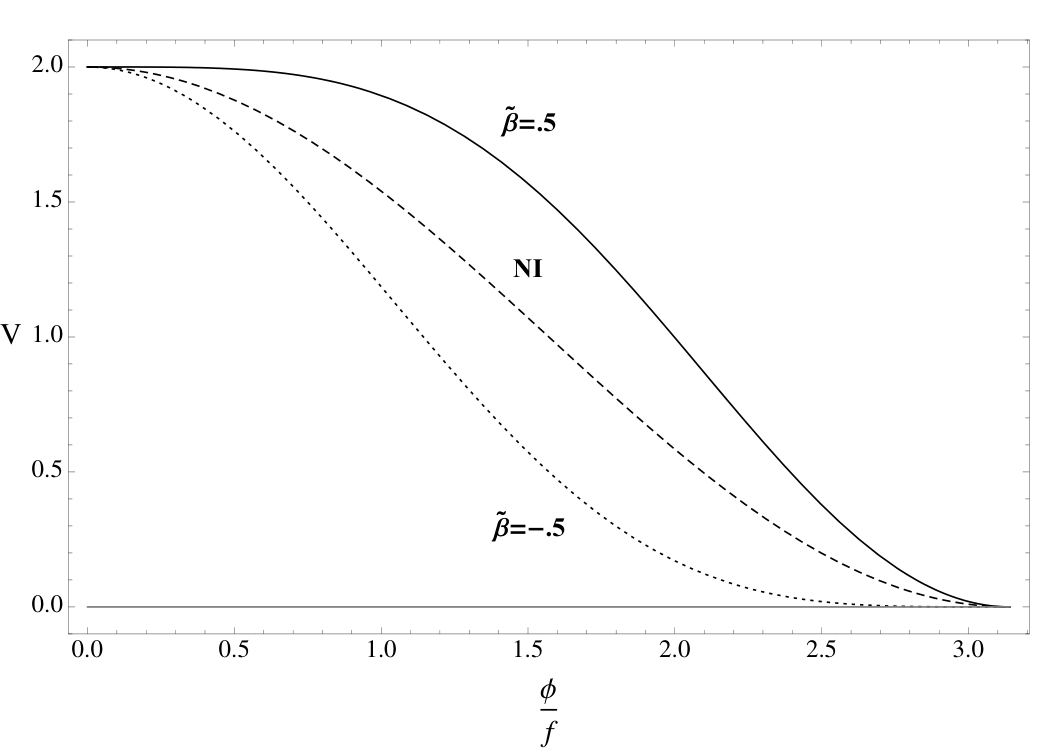
As the Planck data indicates a small deviation from scale invariance, we expect a small deviation of $\tilde{\beta}$ with respect to 1/2. We find that the smaller $f$ compared to $M_{p}$, the closer $\tilde{\beta}$ must be to the values in the table. The deviation $\delta\tilde{\beta}=1/2-\beta$ is then

$$1\times 10^{-2}\left(\frac{f}{M_{p}}\right)^{2}<\,\delta\tilde{\beta}\,<2\times 10^{-2}\left(\frac{f}{M_{p}}\right)^{2}$$

(40)

for all models in the table, but most importantly the model motivated in the previous section (34).

This is the range of $\tilde{\beta}$ for which the model is compatible with the Planck data, as we plot in Fig. 3. for the well motivated example $V=\Lambda^{4}\left(C_{\Lambda}+\alpha\cos\phi/f+\beta\sin^{2}\phi/f\right)$. Our models predict negligible tensors, so the measurement of $r$ imposes no constraint on $\tilde{\beta}$. In fact, the tensor to scalar ratio will scale as

$\displaystyle r\propto\left(\frac{f}{M_{p}}\right)^{4}$

(41)

such that the lower the symmetry breaking scale, the smaller the predicted tensor modes are.

The scale of inflation can be found from the amplitude of the scalar power spectrum, as measured by Planck [2],

$\displaystyle A_{s}=\frac{\Lambda^{4}}{24\pi^{2}M_{p}^{4}\epsilon}=\frac{e^{3.089}}{10^{10}}$

(42)

where $\epsilon=r/16$ is the first slow roll parameter. For our case this implies

$\displaystyle\Lambda_{inf}\approx 10^{15}\left(\frac{f}{M_{p}}\right)\text{GeV}.$

(43)

It is seen that $\Lambda_{inf}$ is expected to be of order of the GUT scale, but can be lower if we allow for tuning. The symmetry breaking should occur before the onset of inflation, and therefore the scale $f$ is expected to lie in the interval $\Lambda_{inf}<f<M_{p}$. Indeed, from the above relation, it is seen that $\Lambda_{inf}\approx 10^{-3}f$. Lowering the scale $f$ as a result of more tuning thus directly results in lowering the scale inflation; for example, the model predicts $f\approx M_{GUT}\rightarrow\Lambda_{inf}\approx 10^{12}\,\text{GeV}$ for $\delta\tilde{\beta}\approx 10^{-6}$. We will quantify the tuning in the model more precisely in the next section.

We saw above that the model (3) gives inflation compatible with the CMB data for particular relations between the coefficients. Here we discuss what these relations indicate for the UV theory.

Firstly, we noticed that to have the right shape of the potential, we should require $\beta$ to be positive, that is

$$\beta=\int\frac{d^{4}p_{E}}{(2\pi\Lambda)^{4}}\left(\frac{3(N-2)}{4}\frac{\Pi_{1}^{A}}{\Pi_{0}^{A}}-2N_{c}\frac{M^{2}}{p_{E}^{2}\Pi_{0}^{L}\Pi_{0}^{R}}\right)>0$$

(62)

Then we saw in Table table that the requirement of a sufficiently flat potential gives the condition $\alpha\approx 2\beta$, which will give a relation between the form factors of the form

	$\displaystyle\alpha$	$\displaystyle=-2N_{c}\int\frac{d^{4}p_{E}}{(2\pi\Lambda)^{4}}\left(\frac{\Pi_{1}^{L}}{\Pi_{0}^{L}}-\frac{\Pi_{1}^{R}}{\Pi_{0}^{R}}\right)$
		$\displaystyle=2\int\frac{d^{4}p_{E}}{(2\pi\Lambda)^{4}}\left(\frac{3(N-2)}{4}\frac{\Pi_{1}^{A}}{\Pi_{0}^{A}}-2N_{c}\frac{M^{2}}{p_{E}^{2}\Pi_{0}^{L}\Pi_{0}^{R}}\right)=2\beta$		(63)

Lastly we have that the phenomenological condition $V(\phi_{min})=0$ gives a preferred value of the constant $C_{\Lambda}$ in terms of the model parameters. In explicit models this will give a condition of the form¹⁰¹⁰ 10 Note that in some models $C_{\Lambda}$ will be related to $\alpha\pm\beta\approx 3/2\,\alpha$, as is seen in Table 3.

$\displaystyle\alpha=-2N_{c}\int\frac{d^{4}p_{E}}{(2\pi\Lambda)^{4}}\left[\frac{\Pi_{1}^{L}}{\Pi_{0}^{L}}-\frac{\Pi_{1}^{R}}{\Pi_{0}^{R}}\right]=C_{\Lambda}$

(64)

where $C_{\Lambda}$ is a cosmological constant during inflation.

To obtain explicit expressions for the form factors $\Pi_{X}$ one would need a UV-complete theory. However, using the relations above we can make some general remarks about their large momentum behaviour. First, we can use an operator product expansion to find the scaling of $\Pi_{1}$. This implies that $\Pi_{1}$ scales as $\langle\mathcal{O}\rangle/p^{d-2}$, where $\mathcal{O}$ is the lowest operator responsible for the breaking $G\rightarrow H$, with mass dimension $d$. In our case, we expect $\mathcal{O}$ to be a fermion condensate with $d=6$. Secondly we can require finiteness of the fermion Lagrangian (27). The scaling of the other form factors can be found by consideration of the kinetic terms in the high momentum limit. We will discuss this in the next section. We summarise our conclusions in Table 4.

References

- (1) A. H. Guth, “The Inflationary Universe: A Possible Solution to the Horizon and Flatness Problems,” Phys. Rev. D 23, 347 (1981).
- (2) P. A. R. Ade et al. [Planck Collaboration], arXiv:1502.02114 [astro-ph.CO].
- (3) D. H. Lyth, Phys. Rev. Lett. 78, 1861 (1997) [hep-ph/9606387]. D. H. Lyth, arXiv:1403.7323 [hep-ph].
- (4) K. Freese, J. A. Frieman and A. V. Olinto, “Natural inflation with pseudo - Nambu-Goldstone bosons,” Phys. Rev. Lett. 65, 3233 (1990). F. C. Adams, J. R. Bond, K. Freese, J. A. Frieman and A. V. Olinto, “Natural inflation: Particle physics models, power law spectra for large scale structure, and constraints from COBE,” Phys. Rev. D 47, 426 (1993) [hep-ph/9207245].
- (5) D. Croon and V. Sanz, JCAP 1502, no. 02, 008 (2015) [arXiv:1411.7809 [hep-ph]].
- (6) P. Svrcek and E. Witten, “Axions In String Theory,” JHEP 0606, 051 (2006) [hep-th/0605206].
- (7) R. Kallosh, A. D. Linde, D. A. Linde and L. Susskind, Phys. Rev. D 52, 912 (1995) [hep-th/9502069].
- (8) M. Montero, A. M. Uranga and I. Valenzuela, arXiv:1503.03886 [hep-th].
- (9) Z. Kenton and S. Thomas, JHEP 1502, 127 (2015) [arXiv:1409.1221 [hep-th]].
- (10) N. Arkani-Hamed, H. C. Cheng, P. Creminelli and L. Randall, “Extra natural inflation,” Phys. Rev. Lett. 90, 221302 (2003) [hep-th/0301218].
- (11) A. D. Linde, “Hybrid inflation,” Phys. Rev. D 49, 748 (1994) [astro-ph/9307002].
- (12) J. E. Kim, H. P. Nilles and M. Peloso, “Completing natural inflation,” JCAP 0501, 005 (2005) [hep-ph/0409138].
- (13) S. Dimopoulos, S. Kachru, J. McGreevy and J. G. Wacker, “N-flation,” JCAP 0808 (2008) 003 [hep-th/0507205].
- (14) A. R. Liddle, A. Mazumdar and F. E. Schunck, Phys. Rev. D 58, 061301 (1998) [astro-ph/9804177]. E. J. Copeland, A. Mazumdar and N. J. Nunes, Phys. Rev. D 60, 083506 (1999) [astro-ph/9904309].
- (15) E. Silverstein and A. Westphal, “Monodromy in the CMB: Gravity Waves and String Inflation,” Phys. Rev. D 78, 106003 (2008) [arXiv:0803.3085 [hep-th]].
- (16) N. Arkani-Hamed, H. C. Cheng, P. Creminelli and L. Randall, “Pseudonatural inflation,” JCAP 0307, 003 (2003) [hep-th/0302034].
- (17) C. Csaki, N. Kaloper, J. Serra and J. Terning, “Inflation from Broken Scale Invariance,” Phys. Rev. Lett. 113 (2014) 161302 [arXiv:1406.5192 [hep-th]].
- (18) R. Contino, Y. Nomura and A. Pomarol, “Higgs as a holographic pseudoGoldstone boson,” Nucl. Phys. B 671 (2003) 148 [hep-ph/0306259].
- (19) C.G. Callan, S. Coleman, J. Wess and B. Zumino, “Structure of Phenomenological Lagrangians. II” Phys. Rev. 177, 2247 (1969).
- (20) G. von Gersdorff, E. Ponton and R. Rosenfeld, arXiv:1502.07340 [hep-ph].
- (21) K. Agashe, R. Contino and A. Pomarol, “The Minimal composite Higgs model,” Nucl. Phys. B 719, 165 (2005) [hep-ph/0412089].
- (22) B. Gripaios, A. Pomarol, F. Riva and J. Serra, “Beyond the Minimal Composite Higgs Model,” JHEP 0904, 070 (2009) [arXiv:0902.1483 [hep-ph]].
- (23) R. Contino, “The Higgs as a Composite Nambu-Goldstone Boson,” arXiv:1005.4269 [hep-ph]. B. Bellazzini, C. Csaki and J. Serra, “Composite Higgses,” Eur. Phys. J. C 74, 2766 (2014) [arXiv:1401.2457 [hep-ph]].
- (24) S. Coleman and E. Weinberg, “Radiative Corrections as the Origin of Spontaneous Symmetry Breaking,” Phys. Rev. D 7, 1888 (1973).
- (25) A. Pomarol and F. Riva, “The Composite Higgs and Light Resonance Connection,” JHEP 1208, 135 (2012) [arXiv:1205.6434 [hep-ph]].
- (26) J. R. Ellis, K. Enqvist, D. V. Nanopoulos and F. Zwirner, Mod. Phys. Lett. A 1, 57 (1986). R. Barbieri and G. F. Giudice, Nucl. Phys. B 306, 63 (1988).
- (27) J. R. Espinosa, C. Grojean, V. Sanz and M. Trott, JHEP 1212, 077 (2012) [arXiv:1207.7355 [hep-ph]].
- (28) J. Gasser and A. Zepeda, Nucl. Phys. B 174 (1980) 445. J. Gasser and H. Leutwyler, Annals Phys. 158 (1984) 142. J. Gasser and H. Leutwyler, Nucl. Phys. B 250 (1985) 465.
- (29) D. Baumann, D. Green, H. Lee and R. A. Porto, arXiv:1502.07304 [hep-th].
- (30) B. Bellazzini, L. Martucci and R. Torre, JHEP 1409, 100 (2014) [arXiv:1405.2960 [hep-th]].
- (31) A. V. Manohar and V. Mateu, Phys. Rev. D 77 (2008) 094019 [arXiv:0801.3222 [hep-ph]]. V. Mateu, Phys. Rev. D 77 (2008) 094020 [arXiv:0801.3627 [hep-ph]]. A. Filipuzzi, J. Portoles and P. Ruiz-Femenia, JHEP 1208 (2012) 080 [arXiv:1205.4682 [hep-ph]]. J. J. Sanz-Cillero, D. L. Yao and H. Q. Zheng, Eur. Phys. J. C 74 (2014) 2763 [arXiv:1312.0664 [hep-ph]].
- (32) G. Ecker, J. Gasser, A. Pich and E. de Rafael, Nucl. Phys. B 321 (1989) 311. G. Ecker, J. Gasser, H. Leutwyler, A. Pich and E. de Rafael, Phys. Lett. B 223 (1989) 425.
- (33) R. Lewis, C. Pica and F. Sannino, Phys. Rev. D 85 (2012) 014504 [arXiv:1109.3513 [hep-ph]].
- (34) D. Baumann and D. Green, JCAP 1109, 014 (2011) [arXiv:1102.5343 [hep-th]].
- (35) D. Baumann, D. Green and R. A. Porto, JCAP 1501, no. 01, 016 (2015) [arXiv:1407.2621 [hep-th]].
- (36) G. ’t Hooft (1980). "Naturalness, Chiral Symmetry and Spontaneous Chiral Symmetry Breaking". In G ’t Hooft, Recent Developments in Gauge Theories. Plenum Press.
- (37) G. ’t Hooft, “A planar diagram theory for strong interactions,” Nucl. Phys. B 72, 461 (1974); B 75, 461 (1974).
- (38) E. Witten, “Baryons in the 1/N expansion”, Nucl. Phys. B 160, 57 (1979).
- (39) S. Weinberg, “Precise Relations between the Spectra of Vector and Axial-Vector Mesons,” Phys. Rev. Lett. 18 (1967) 507
- (40) M. Knecht and E. de Rafael, “Patterns of spontaneous chiral symmetry breaking in the large N(c) limit of QCD - like theories,” Phys. Lett. B 424, 335 (1998) [hep-ph/9712457].
- (41) P. A. R. Ade et al. [Planck Collaboration], arXiv:1502.02114 [astro-ph.CO].
- (42) G. von Gersdorff, E. Ponton and R. Rosenfeld, arXiv:1502.07340 [hep-ph].
- (43) B. Bellazzini, C. Csaki and J. Serra, Eur. Phys. J. C 74 (2014) 5, 2766 [arXiv:1401.2457 [hep-ph]].
- (44) A. Martin and V. Sanz, JHEP 1001 (2010) 075 [arXiv:0907.3931 [hep-ph]]. J. Hirn, A. Martin and V. Sanz, Phys. Rev. D 78 (2008) 075026 [arXiv:0807.2465 [hep-ph]]. JHEP 0805 (2008) 084 [arXiv:0712.3783 [hep-ph]].
- (45) G. Cacciapaglia, C. Csaki, C. Grojean and J. Terning, Phys. Rev. D 71 (2005) 035015 [hep-ph/0409126]. K. Agashe, C. Csaki, C. Grojean and M. Reece, JHEP 0712 (2007) 003 [arXiv:0704.1821 [hep-ph]].
- (46) J. Hirn and V. Sanz, Phys. Rev. Lett. 97 (2006) 121803 [hep-ph/0606086]. JHEP 0703 (2007) 100 [hep-ph/0612239].
- (47) N. Kaloper, A. Lawrence and L. Sorbo, “An Ignoble Approach to Large Field Inflation,” JCAP 1103, 023 (2011) [arXiv:1101.0026 [hep-th]]. X. Calmet and V. Sanz, Phys. Lett. B 737, 12 (2014) [arXiv:1403.5100 [hep-ph]].
- (48) W. H. Kinney and K. T. Mahanthappa, Phys. Rev. D 53 (1996) 5455 [hep-ph/9512241].
- (49) A. Jokinen and A. Mazumdar, Phys. Lett. B 597 (2004) 222 [hep-th/0406074].