Schwinger’s Quantum Action Principle

From Dirac’s formulation through Feynman’s path integrals, the Schwinger-Keldysh method, quantum field theory, to source theory

Kimball A. Milton

Abstract

Starting from the earlier notions of stationary action principles, we show how Julian Schwinger’s Quantum Action Principle descended from Dirac’s formulation, which independently led Feynman to his path-integral formulation of quantum mechanics. The connection between the two is brought out, and applications are discussed. The Keldysh-Schwinger time-cycle method of extracting matrix elements in nonequilibrium situations is described. The variational formulation of quanum field theory and the development of source theory constitute the latter part of this work. In this document, derived from Schwinger’s lectures over four decades, the continuity of concepts, such as that of Green’s functions, becomes apparent.

\frontmatter

\mainmatter

Chapter \thechapter Historical Introduction

Variational principles for dynamical systems have a long history. Although precursors go back at least to Leibnitz (see for example Euler (1752)) and Euler Euler (1744) the “principle of least action” was given modern form by de Maupertuis Maupertuis (1744); Maupertuis (1746). We will not attempt to trace the history here; a brief useful account is given in Sommerfeld’s lectures Sommerfeld (1964). The most important names in the history of the development of dynamical systems, or at least those that will bear most directly on the following discussion, are those of Joseph-Louis Lagrange Lagrange (1788) and William Rowan Hamilton Hamilton (1834); Hamilton (1835).

Here we are concentrating on the work of Julian Schwinger (1918--1994), who had profound and pervasive influence on 20th century physics, and whose many students have become leaders in diverse fields.¹¹ 1 For complex reasons, Schwinger’s influence on modern physics is not widely appreciated. His contributions to our current understanding of nature are underrepresented in textbooks, with some notable exceptions Toms (2007). For biographical information about his life and work see Mehra (2000); Milton (2007). Therefore, we will take up the story in the modern era. Shortly after Dirac’s work with Fock and Podolsky Dirac (1932), in which the demonstration of the equivalence between his theory of quantum electrodynamics, and that of Heisenberg and Pauli Heisenberg (1929), P. A. M. Dirac wrote a paper on “The Lagrangian in Quantum Mechanics” Dirac (1933). This paper had a profound influence on Richard Feynman’s doctoral dissertation at Princeton on “The Principles of Least Action in Quantum Mechanics” Feynman (1942), and on his later work on the formulations of the “Space-Time Approach to Quantum Electrodynamics” Feynman (1949). Dirac’s paper further formed the basis for Schwinger’s development of the quantum action principle, which first appeared in his final operator field formulation of quantum field theory Schwinger 1951b (), which we will describe in Chapter 6.

The response of Feynman and Schwinger to Dirac’s inspiring paper was completely different. Feynman was to give a global “solution” to the problem of determining the transformation function, the probability amplitude connecting the state of the system at one time to that at a later time, in terms of a sum over classical trajectories, the famous path integral. Schwinger, instead, derived (initially postulated) a differential equation for that transformation function in terms of a quantum action functional. This differential equation possessed Feynman’s path integral as a formal solution, which remained poorly defined; but Schwinger believed throughout his life that his approach was “more general, more elegant, more useful, and more tied to the historical line of development as the quantum transcription of Hamilton’s action principle” Schwinger (1973).

Later, in a tribute to Feynman, Schwinger commented further. Dirac, of course, was the father of transformation theory Dirac (1927). The transformation function from a description of the system at time $t_{2}$ to a description at time $t_{1}$ is “the product of all the transformations functions associated with the successive infinitesimal increments in time.” Dirac said the latter, that is, the transformation function from time $t$ to time $t+dt$ corresponds to $\exp[(i/\hbar)dt\,L]$ , where $L$ is the Lagrangian expressed in terms of the coordinates at the two times. For the transformation function between $t_{2}$ and $t_{1}$ “the integrand is $\exp[(i/\hbar)W]$ . where $W=\int_{t_{2}}^{t_{1}}dt\,L$ .” “Now we know, and Dirac surely knew, that to within a constant factor the ‘correspondence,’ for infinitesimal $dt$ , is an equality when we deal with a system of nonrelativistic particles possessing a coordinate-dependent potential energy $V$ …. Why then, did Dirac not make a more precise, if less general statement? Because he was interested in a general question: What, in quantum mechanics, corresponds to the classical principle of stationary action?”

“Why, in the decade that followed, didn’t someone pick up the computational possibilities offered by this integral approach to the time transformation function? To answer this question bluntly, perhaps no one needed it—until Feynman came along.” Schwinger 1989a ().

But Schwinger followed the differential route, and starting in early 1950 began a new, his third, formulation of quantum electrodynamics, based on a variational approach. This was first published in 1951 Schwinger 1951b (). A bit later he started developing a new formulation of quantum kinematics, which he called Measurement Algebra, which got its first public presentation at École de Physique des Houches in the summer of 1955. There were several short notes in the Proceedings of the US National Academy published in 1960, explaining both the quantum kinematical approach and the dynamical action principle Schwinger 1960a (); Schwinger 1960b (); Schwinger 1960c (); Schwinger 1960d (), but although he often promised to write a book on the subject (as he also promised a book on quantum field theory) nothing came of it. Les Houches lectures, based on notes taken by Robert Kohler, eventually appeared in 1970 Schwinger 1970a (). Lectures based on a UCLA course on quantum mechanics by Schwinger were eventually published under Englert’s editorship Schwinger (2001). The incompleteness of the written record may be partly alleviated by the present essay.

We start on a classical footing.

Chapter \thechapter Review of Classical Action Principles

This section grew out of lectures given by Schwinger at UCLA around 1974, which were substantially transformed into Chapter 8 of Classical Electrodynamics Schwinger (1998). (Remarkably, considering his work on waveguide theory during World War II, now partially recorded in Ref. Milton (2006), he never gave lectures on this subject at Harvard after 1947.)

We start by reviewing and generalizing the Lagrange-Hamilton principle for a single particle. The action, $W_{12}$ , is defined as the time integral of the Lagrangian, $L$ , where the integration extends from an initial configuration or state at time $t_{2}$ to a final state at time $t_{1}$ :

W_{12}=\int_{t_{2}}^{t_{1}}dt\,L.

(1)

The integral refers to any path, any line of time development, from the initial to the final state, as shown in Fig. 1.

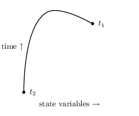
Refer to caption — Figure 1: A possible path from initial state to final state.

The actual time evolution of the system is selected by the principle of stationary action: In response to infinitesimal variations of the integration path, the action $W_{12}$ is stationary—does not have a corresponding infinitesimal change—for variations about the correct path, provided the initial and final configurations are held fixed,

\delta W_{12}=0.

(2)

This means that, if we allow infinitesimal changes at the initial and final times, including alterations of those times, the only contribution to $\delta W_{12}$ then comes from the endpoint variations, or

\delta W_{12}=G_{1}-G_{2},

(3)

where $G_{a}$ , $a=1$ or $2$ , is a function, called the generator, depending on dynamical variables only at time $t_{a}$ . In the following, we will consider three different realizations of the action principle, where, for simplicity, we will restrict our attention to a single particle.

1 Lagrangian Viewpoint

The nonrelativistic motion of a particle of mass $m$ moving in a potential $V({\bf r},t)$ is described by the Lagrangian

L={1\over 2}m\left({d{\bf r}\over dt}\right)^{2}-V({\bf r},t).

(4)

Here, the independent variables are $\bf r$ and $t$ , so that two kinds of variations can be considered. First, a particular motion is altered infinitesimally, that is, the path is changed by an amount $\delta{\bf r}$ :

{\bf r}(t)\to{\bf r}(t)+\delta{\bf r}(t).

(5)

Second, the final and initial times can be altered infinitesimally, by $\delta t_{1}$ and $\delta t_{2}$ , respectively. It is more convenient, however, to think of these time displacements as produced by a continuous variation of the time parameter, $\delta t(t)$ ,

t\to t+\delta t(t),

(6)

so chosen that, at the endpoints,

\delta t(t_{1})=\delta t_{1},\qquad\delta t(t_{2})=\delta t_{2}.

(7)

The corresponding change in the time differential is

dt\to d(t+\delta t)=\left(1+{d\delta t\over dt}\right)dt,

(8)

which implies the transformation of the time derivative,

{d\over dt}\to\left(1-{d\delta t\over dt}\right){d\over dt}.

(9)

Because of this redefinition of the time variable, the limits of integration in the action,

W_{12}=\int_{2}^{1}\left[{1\over 2}m{(d{\bf r})^{2}\over dt}-dt\,V\right],

(10)

are not changed, the time displacement being produced through $\delta t(t)$ subject to (7). The resulting variation in the action is now

$\displaystyle\delta W_{12}$	$\displaystyle=$	$\displaystyle\int_{2}^{1}dt\left\{m{d{\bf r}\over dt}\raisebox{-1.99168pt}{\hskip 1.13809pt\LARGE$\cdot$\hskip 1.13809pt}{d\over dt}\delta{\bf r}-\delta{\bf r}\raisebox{-1.99168pt}{\hskip 1.13809pt\LARGE$\cdot$\hskip 1.13809pt}\mbox{\boldmath{$\nabla$}}V-{d\delta t\over dt}\left[{1\over 2}m\left({d{\bf r}\over dt}\right)^{2}+V\right]-\delta t{\partial\over\partial t}V\right\}$
	$\displaystyle=$	$\displaystyle\int_{2}^{1}dt\Bigg\{{d\over dt}\left[m{d{\bf r}\over dt}\raisebox{-1.99168pt}{\hskip 1.13809pt\LARGE$\cdot$\hskip 1.13809pt}\delta{\bf r}-\left({1\over 2}m\left({d{\bf r}\over dt}\right)^{2}+V\right)\delta t\right]$
		$\displaystyle\!\!\!\!\!\mbox{}+\delta{\bf r}\raisebox{-1.99168pt}{\hskip 1.13809pt\LARGE$\cdot$\hskip 1.13809pt}\left[-m{d^{2}\over dt^{2}}{\bf r}-\mbox{\boldmath{$\nabla$}}V\right]+\delta t\left({d\over dt}\left[{1\over 2}m\left({d{\bf r}\over dt}\right)^{2}+V\right]-{\partial\over\partial t}V\right)\!\!\!\Bigg\},$

where, in the last form, we have integrated by parts in order to isolate $\delta{\bf r}$ and $\delta t$ .

Because $\delta{\bf r}$ and $\delta t$ are independent variations, the principle of stationary action implies that the actual motion is governed by


	$\displaystyle m{d^{2}\over dt^{2}}{\bf r}=$	$\displaystyle-$	$\displaystyle\mbox{\boldmath{$\nabla$}}V,$	(12a)
	$\displaystyle{d\over dt}\bigg[{1\over 2}m\left({d{\bf r}\over dt}\right)^{2}$	$\displaystyle+$	$\displaystyle V\bigg]={\partial\over\partial t}V,$	(12b)
while the total time derivative gives the change at the endpoints,
	$G={\bf p\raisebox{-1.99168pt}{\hskip 1.13809pt\LARGE$\cdot$\hskip 1.13809pt}\delta r}-E\delta t,$			(12c)
with
	$\mbox{momentum}={\bf p}=m{d{\bf r}\over dt},\qquad\mbox{energy}=E={1\over 2}m\left({d{\bf r}\over dt}\right)^{2}+V.$			(12d)

Therefore, we have derived Newton’s second law [the equation of motion in second-order form], (12a), and, for a static potential, $\partial V/\partial t=0$ , the conservation of energy, (12b). The significance of (12c) will be discussed later in Section 4.

2 Hamiltonian Viewpoint

Using the above definition of the momentum, we can rewrite the Lagrangian as

L={\bf p}\raisebox{-1.99168pt}{\hskip 1.13809pt\LARGE$\cdot$\hskip 1.13809pt}{d{\bf r}\over dt}-H({\bf r},{\bf p},t),

(13)

where we have introduced the Hamiltonian

H={p^{2}\over 2m}+V({\bf r},t).

(14)

We are here to regard $\bf r$ , $\bf p$ , and $t$ as independent variables in

W_{12}=\int_{2}^{1}[{\bf p}\raisebox{-1.99168pt}{\hskip 1.13809pt\LARGE$\cdot$\hskip 1.13809pt}d{\bf r}-dt\,H].

(15)

The change in the action, when $\bf r$ , $\bf p$ , and $t$ are all varied, is

$\displaystyle\delta W_{12}$	$\displaystyle=$	$\displaystyle\int_{2}^{1}dt\left[{\bf p}\raisebox{-1.99168pt}{\hskip 1.13809pt\LARGE$\cdot$\hskip 1.13809pt}{d\over dt}\delta{\bf r}-\delta{\bf r}\raisebox{-1.99168pt}{\hskip 1.13809pt\LARGE$\cdot$\hskip 1.13809pt}{\partial H\over\partial{\bf r}}+\delta{\bf p}\raisebox{-1.99168pt}{\hskip 1.13809pt\LARGE$\cdot$\hskip 1.13809pt}{d{\bf r}\over dt}-\delta{\bf p}\raisebox{-1.99168pt}{\hskip 1.13809pt\LARGE$\cdot$\hskip 1.13809pt}{\partial H\over\partial{\bf p}}-{d\delta t\over dt}H-\delta t{\partial H\over\partial t}\right]$	(16)
	$\displaystyle=$	$\displaystyle\int_{2}^{1}dt\bigg[{d\over dt}({\bf p\raisebox{-1.99168pt}{\hskip 1.13809pt\LARGE$\cdot$\hskip 1.13809pt}\delta r}-H\delta t)+\delta{\bf r}\raisebox{-1.99168pt}{\hskip 1.13809pt\LARGE$\cdot$\hskip 1.13809pt}\left(-{d{\bf p}\over dt}-{\partial H\over\partial{\bf r}}\right)$
		$\displaystyle\quad+\delta{\bf p}\raisebox{-1.99168pt}{\hskip 1.13809pt\LARGE$\cdot$\hskip 1.13809pt}\left({d{\bf r}\over dt}-{\partial H\over\partial{\bf p}}\right)+\delta t\left({dH\over dt}-{\partial H\over\partial t}\right)\bigg].$

The action principle then implies


$\displaystyle{d{\bf r}\over dt}$	$\displaystyle=$	$\displaystyle{\partial H\over\partial{\bf p}}={{\bf p}\over m},$	(17a)
$\displaystyle{d{\bf p}\over dt}$	$\displaystyle=$	$\displaystyle-{\partial H\over\partial{\bf r}}=-\mbox{\boldmath{$\nabla$}}V,$	(17b)
$\displaystyle{dH\over dt}$	$\displaystyle=$	$\displaystyle{\partial H\over\partial t},$	(17c)
$\displaystyle G$	$\displaystyle=$	$\displaystyle{\bf p\raisebox{-1.99168pt}{\hskip 1.13809pt\LARGE$\cdot$\hskip 1.13809pt}\delta r}-H\delta t.$	(17d)

In contrast with the Lagrangian differential equations of motion, which involve second derivatives, these Hamiltonian equations contain only first derivatives; they are called first-order equations. They describe the same physical system, because when (17a) is substituted into (17b), we recover the Lagrangian-Newtonian equation (12a). Furthermore, if we insert (17a) into the Hamiltonian (14), we identify $H$ with $E$ . The third equation (17c) is then identical with (12b). We also note the equivalence of the two versions of $G$ .

But probably the most direct way of seeing that the same physical system is involved comes by writing the Lagrangian in the Hamiltonian viewpoint as

L={m\over 2}\left({d{\bf r}\over dt}\right)^{2}-V-{1\over 2m}\left({\bf p}-m{d{\bf r}\over dt}\right)^{2}.

(18)

The result of varying $\bf p$ in the stationary action principle is to produce

{\bf p}=m{d{\bf r}\over dt}.

(19)

But, if we accept this as the definition of $\bf p$ , the corresponding term in $L$ disappears and we explicitly regain the Lagrangian description. We are justified in completely omitting the last term on the right side of (18), despite its dependence on the variables $\bf r$ and $t$ , because of its quadratic structure. Its explicit contribution to $\delta L$ is

-{1\over m}\left({\bf p}-m{d{\bf r}\over dt}\right)\raisebox{-1.99168pt}{\hskip 1.13809pt\LARGE$\cdot$\hskip 1.13809pt}\left(\delta{\bf p}-m{d\over dt}\delta{\bf r}+m{d{\bf r}\over dt}{d\delta t\over dt}\right),

(20)

and the equation supplied by the stationary action principle for $\bf p$ variations, (19), also guarantees that there is no contribution here to the results of $\bf r$ and $t$ variations.

3 A Third, Schwingerian, Viewpoint

Here we take $\bf r$ , $\bf p$ , and the velocity, $\bf v$ , as independent variables, so that the Lagrangian is written in the form

L={\bf p}\raisebox{-1.99168pt}{\hskip 1.13809pt\LARGE$\cdot$\hskip 1.13809pt}\left({d{\bf r}\over dt}-{\bf v}\right)+{1\over 2}mv^{2}-V({\bf r},t)\equiv{\bf p}\raisebox{-1.99168pt}{\hskip 1.13809pt\LARGE$\cdot$\hskip 1.13809pt}{d{\bf r}\over dt}-H({\bf r,p,v},t),

(21)

where

H({\bf r,p,v},t)={\bf p\raisebox{-1.99168pt}{\hskip 1.13809pt\LARGE$\cdot$\hskip 1.13809pt}v}-{1\over 2}mv^{2}+V({\bf r},t).

(22)

The variation of the action is now

$\displaystyle\delta W_{12}$	$\displaystyle=$	$\displaystyle\delta\int_{2}^{1}[{\bf p}\raisebox{-1.99168pt}{\hskip 1.13809pt\LARGE$\cdot$\hskip 1.13809pt}d{\bf r}-H\,dt]$	(23)
	$\displaystyle=$	$\displaystyle\int_{2}^{1}dt\bigg[\delta{\bf p}\raisebox{-1.99168pt}{\hskip 1.13809pt\LARGE$\cdot$\hskip 1.13809pt}{d{\bf r}\over dt}+{\bf p}\raisebox{-1.99168pt}{\hskip 1.13809pt\LARGE$\cdot$\hskip 1.13809pt}{d\over dt}\delta{\bf r}-\delta{\bf r}\raisebox{-1.99168pt}{\hskip 1.13809pt\LARGE$\cdot$\hskip 1.13809pt}{\partial H\over\partial{\bf r}}-\delta{\bf p}\raisebox{-1.99168pt}{\hskip 1.13809pt\LARGE$\cdot$\hskip 1.13809pt}{\partial H\over\partial{\bf p}}-\delta{\bf v}\raisebox{-1.99168pt}{\hskip 1.13809pt\LARGE$\cdot$\hskip 1.13809pt}{\partial H\over\partial{\bf v}}$
		$\displaystyle\qquad\mbox{}-\delta t{\partial H\over\partial t}-H{d\delta t\over dt}\bigg]$
	$\displaystyle=$	$\displaystyle\int_{2}^{1}dt\bigg[{d\over dt}({\bf p\raisebox{-1.99168pt}{\hskip 1.13809pt\LARGE$\cdot$\hskip 1.13809pt}\delta r}-H\delta t)-\delta{\bf r}\raisebox{-1.99168pt}{\hskip 1.13809pt\LARGE$\cdot$\hskip 1.13809pt}\left({d{\bf p}\over dt}+{\partial H\over\partial{\bf r}}\right)$
		$\displaystyle\mbox{}+\delta{\bf p}\raisebox{-1.99168pt}{\hskip 1.13809pt\LARGE$\cdot$\hskip 1.13809pt}\left({d{\bf r}\over dt}-{\partial H\over\partial{\bf p}}\right)-\delta{\bf v}\raisebox{-1.99168pt}{\hskip 1.13809pt\LARGE$\cdot$\hskip 1.13809pt}{\partial H\over\partial{\bf v}}+\delta t\left({dH\over dt}-{\partial H\over\partial t}\right)\bigg],$

so that the action principle implies


$\displaystyle{d{\bf p}\over dt}$	$\displaystyle=$	$\displaystyle-{\partial H\over\partial{\bf r}}=-\mbox{\boldmath{$\nabla$}}V,$	(24a)
$\displaystyle{d{\bf r}\over dt}$	$\displaystyle=$	$\displaystyle{\partial H\over\partial{\bf p}}={\bf v},$	(24b)
$\displaystyle{\bf 0}$	$\displaystyle=$	$\displaystyle-{\partial H\over\partial{\bf v}}=-{\bf p}+m{\bf v},$	(24c)
$\displaystyle{dH\over dt}$	$\displaystyle=$	$\displaystyle{\partial H\over\partial t},$	(24d)
$\displaystyle G$	$\displaystyle=$	$\displaystyle{\bf p\raisebox{-1.99168pt}{\hskip 1.13809pt\LARGE$\cdot$\hskip 1.13809pt}\delta r}-H\delta t.$	(24e)

Notice that there is no equation of motion for $\bf v$ since $d{\bf v}/dt$ does not occur in the Lagrangian, nor is it multiplied by a time derivative. Consequently, (24c) refers to a single time and is an equation of constraint.

From this third approach, we have the option of returning to either of the other two viewpoints by imposing an appropriate restriction. Thus, if we write (22) as

H({\bf r,p,v},t)={p^{2}\over 2m}+V({\bf r},t)-{1\over 2m}({\bf p}-m{\bf v})^{2},

(25)

and we adopt

{\bf v}={1\over m}{\bf p}

(26)

as the definition of $\bf v$ , we recover the Hamiltonian description, (13) and (14). Alternatively, we can present the Lagrangian (21) as

L={m\over 2}\left(d{\bf r}\over dt\right)^{2}-V+({\bf p}-m{\bf v})\raisebox{-1.99168pt}{\hskip 1.13809pt\LARGE$\cdot$\hskip 1.13809pt}\left({d{\bf r}\over dt}-{\bf v}\right)-{m\over 2}\left({d{\bf r}\over dt}-{\bf v}\right)^{2}.

(27)

Then, if we adopt the following as definitions,

{\bf v}={d{\bf r}\over dt},\quad{\bf p}=m{\bf v},

(28)

the resultant form of $L$ is that of the Lagrangian viewpoint, (4). It might seem that only the definition ${\bf v}=d{\bf r}/dt$ , inserted in (27), suffices to regain the Lagrangian description. But then the next to last term in (27) would give the following additional contribution to $\delta L$ , associated with the variation $\delta{\bf r}$ :

({\bf p}-m{\bf v})\raisebox{-1.99168pt}{\hskip 1.13809pt\LARGE$\cdot$\hskip 1.13809pt}{d\over dt}\delta{\bf r}.

(29)

In the next Chapter, where the action formulation of electrodynamics is considered, we will see the advantage of adopting this third approach, which is characterized by the introduction of additional variables, similar to $\bf v$ , for which there are no equations of motion.

4 Invariance and Conservation Laws

There is more content to the principle of stationary action than equations of motion. Suppose one considers a variation such that

\delta W_{12}=0,

(30)

independently of the choice of initial and final times. We say that the action, which is left unchanged, is invariant under this alteration of path. Then the stationary action principle (3) asserts that

\delta W_{12}=G_{1}-G_{2}=0,

(31)

or, there is a quantity $G(t)$ that has the same value for any choice of time $t$ ; it is conserved in time. A differential statement of that is

{d\over dt}G(t)=0.

(32)

The $G$ functions, which are usually referred to as generators, express the interrelation between conservation laws and invariances of the system.

Invariance implies conservation, and vice versa. A more precise statement is the following:

If there is a conservation law, the action is stationary under an infinitesimal transformation in an appropriate variable.

The converse of this statement is also true.

If the action $W$ is invariant under an infinitesimal transformation (that is, $\delta W=0$ ), then there is a corresponding conservation law.

This is the celebrated theorem of Amalie Emmy Noether Noether (1918).

Here are some examples. Suppose the Hamiltonian of (13) does not depend explicitly on time, or

W_{12}=\int_{2}^{1}[{\bf p}\raisebox{-1.99168pt}{\hskip 1.13809pt\LARGE$\cdot$\hskip 1.13809pt}d{\bf r}-H({\bf r,p})dt].

(33)

Then the variation (which as a rigid displacement in time, amounts to a shift in the time origin)

\delta t=\mbox{constant}

(34)

will give $\delta W_{12}=0$ [see the first line of (16), with $\delta{\bf r}=0$ , $\delta{\bf p}=0$ , $d\delta t/dt=0$ , $\partial H/\partial t=0$ ]. The conclusion is that $G$ in (17d), which here is just

G_{t}=-H\delta t,

(35)

is a conserved quantity, or that

{dH\over dt}=0.

(36)

This inference, that the Hamiltonian—the energy—is conserved, if there is no explicit time dependence in $H$ , is already present in (17c). But now a more general principle is at work.

Next, consider an infinitesimal, rigid rotation, one that maintains the lengths and scalar products of all vectors. Written explicitly for the position vector $\bf r$ , it is

\delta{\bf r}=\delta\vec{\omega}\mbox{\boldmath{$\times$}}{\bf r},

(37)

where the constant vector $\delta\vec{\omega}$ gives the direction and magnitude of the rotation (see Fig. 2).

Now specialize (14) to

H={p^{2}\over 2m}+V(r),

(38)

where $r=|{\bf r}|$ , a rotationally invariant structure. Then

W_{12}=\int_{2}^{1}[{\bf p}\raisebox{-1.99168pt}{\hskip 1.13809pt\LARGE$\cdot$\hskip 1.13809pt}d{\bf r}-H\,dt]

(39)

is also invariant under the rigid rotation, implying the conservation of

G_{\delta\vec{\omega}}={\bf p\raisebox{-1.99168pt}{\hskip 1.13809pt\LARGE$\cdot$\hskip 1.13809pt}\delta r=\delta\vec{\omega}\raisebox{-1.99168pt}{\hskip 1.13809pt\LARGE$\cdot$\hskip 1.13809pt}r\mbox{\boldmath{$\times$}}p.}

(40)

This is the conservation of angular momentum,

{\bf L=r\mbox{\boldmath{$\times$}}p},\quad{d\over dt}{\bf L=0}.

(41)

Of course, this is also contained within the equation of motion,

{d\over dt}{\bf L}=-{\bf r}\mbox{\boldmath{$\times$}}\mbox{\boldmath{$\nabla$}}V=-{\bf r\mbox{\boldmath{$\times$}}\hat{r}}{\partial V\over\partial r}={\bf 0},

(42)

since $V$ depends only on $|{\bf r}|$ .

Conservation of linear momentum appears analogously when there is invariance under a rigid translation. For a single particle, (17b) tells us immediately that $\bf p$ is conserved if $V$ is a constant, say zero. Then, indeed, the action

W_{12}=\int_{2}^{1}\left[{\bf p}\raisebox{-1.99168pt}{\hskip 1.13809pt\LARGE$\cdot$\hskip 1.13809pt}d{\bf r}-{p^{2}\over 2m}dt\right]

(43)

is invariant under the displacement

\delta{\bf r}=\delta\mbox{\boldmath{$\epsilon$}}=\mbox{constant},

(44)

and

G_{\delta\vec{\epsilon}}={\bf p}\raisebox{-1.99168pt}{\hskip 1.13809pt\LARGE$\cdot$\hskip 1.13809pt}\delta\mbox{\boldmath{$\epsilon$}}

(45)

is conserved. But the general principle acts just as easily for, say, a system of two particles, $a$ and $b$ , with Hamiltonian

H={p_{a}^{2}\over 2m_{a}}+{p_{b}^{2}\over 2m_{b}}+V({\bf r}_{a}-{\bf r}_{b}).

(46)

This Hamiltonian and the associated action

W_{12}=\int_{2}^{1}[{\bf p}_{a}\raisebox{-1.99168pt}{\hskip 1.13809pt\LARGE$\cdot$\hskip 1.13809pt}d{\bf r}_{a}+{\bf p}_{b}\raisebox{-1.99168pt}{\hskip 1.13809pt\LARGE$\cdot$\hskip 1.13809pt}d{\bf r}_{b}-H\,dt]

(47)

are invariant under the rigid translation

\delta{\bf r}_{a}=\delta{\bf r}_{b}=\delta\mbox{\boldmath{$\epsilon$}},

(48)

with the implication that

G_{\delta\mbox{\boldmath{$\epsilon$}}}={\bf p}_{a}\raisebox{-1.99168pt}{\hskip 1.13809pt\LARGE$\cdot$\hskip 1.13809pt}\delta{\bf r}_{a}+{\bf p}_{b}\raisebox{-1.99168pt}{\hskip 1.13809pt\LARGE$\cdot$\hskip 1.13809pt}\delta{\bf r}_{b}=({\bf p}_{a}+{\bf p}_{b})\raisebox{-1.99168pt}{\hskip 1.13809pt\LARGE$\cdot$\hskip 1.13809pt}\delta\mbox{\boldmath{$\epsilon$}}

(49)

is conserved. This is the conservation of the total linear momentum,

{\bf P}={\bf p}_{a}+{\bf p}_{b},\quad{d\over dt}{\bf P=0}.

(50)

Something a bit more general appears when we consider a rigid translation that grows linearly in time:

\delta{\bf r}_{a}=\delta{\bf r}_{b}=\delta{\bf v}\,t,

(51)

using the example of two particles. This gives each particle the common additional velocity $\delta{\bf v}$ , and therefore must also change their momenta,

\delta{\bf p}_{a}=m_{a}\delta{\bf v},\quad\delta{\bf p}_{b}=m_{b}\delta{\bf v}.

(52)

The response of the action (47) to this variation is

	$\displaystyle\delta W_{12}$	$\displaystyle=$	$\displaystyle\int_{2}^{1}[({\bf p}_{a}+{\bf p}_{b})\raisebox{-1.99168pt}{\hskip 1.13809pt\LARGE$\cdot$\hskip 1.13809pt}\delta{\bf v}\,dt+\delta{\bf v}\raisebox{-1.99168pt}{\hskip 1.13809pt\LARGE$\cdot$\hskip 1.13809pt}(m_{a}d{\bf r}_{a}+m_{b}d{\bf r}_{b})-({\bf p}_{a}+{\bf p}_{b})\raisebox{-1.99168pt}{\hskip 1.13809pt\LARGE$\cdot$\hskip 1.13809pt}\delta{\bf v}\,dt]$		(53)
		$\displaystyle=$	$\displaystyle\int_{2}^{1}d[(m_{a}{\bf r}_{a}+m_{b}{\bf r}_{b})\raisebox{-1.99168pt}{\hskip 1.13809pt\LARGE$\cdot$\hskip 1.13809pt}\delta{\bf v}].$		(53)

The action is not invariant; its variation has end-point contributions. But there is still a conservation law, not of $G={\bf P\raisebox{-1.99168pt}{\hskip 1.13809pt\LARGE$\cdot$\hskip 1.13809pt}\delta v}t$ , but of ${\bf N}\raisebox{-1.99168pt}{\hskip 1.13809pt\LARGE$\cdot$\hskip 1.13809pt}\delta{\bf v}$ , where

{\bf N=P}t-(m_{a}{\bf r}_{a}+m_{b}{\bf r}_{b}).

(54)

Written in terms of the center-of-mass position vector

{\bf R}={m_{a}{\bf r}_{a}+m_{b}{\bf r}_{b}\over M},\quad M=m_{a}+m_{b},

(55)

the statement of conservation of

{\bf N=P}t-M{\bf R},

(56)

namely

{\bf 0}={d{\bf N}\over dt}={\bf P}-M{d{\bf R}\over dt},

(57)

is the familiar fact that the center of mass of an isolated system moves at the constant velocity given by the ratio of the total momentum to the total mass of that system.

5 Nonconservation Laws. The Virial Theorem

The action principle also supplies useful nonconservation laws. Consider, for constant $\delta\lambda$ ,

\delta{\bf r}=\delta\lambda{\bf r},\quad\delta{\bf p}=-\delta\lambda{\bf p},

(58)

which leaves ${\bf p}\raisebox{-1.99168pt}{\hskip 1.13809pt\LARGE$\cdot$\hskip 1.13809pt}d{\bf r}$ invariant,

\delta({\bf p}\raisebox{-1.99168pt}{\hskip 1.13809pt\LARGE$\cdot$\hskip 1.13809pt}d{\bf r})=(-\delta\lambda{\bf p})\raisebox{-1.99168pt}{\hskip 1.13809pt\LARGE$\cdot$\hskip 1.13809pt}d{\bf r}+{\bf p}\raisebox{-1.99168pt}{\hskip 1.13809pt\LARGE$\cdot$\hskip 1.13809pt}(\delta\lambda d{\bf r})=0.

(59)

But the response of the Hamiltonian

H=T(p)+V({\bf r}),\quad T(p)={p^{2}\over 2m},

(60)

is given by the noninvariant form

\delta H=\delta\lambda(-2T+{\bf r}\raisebox{-1.99168pt}{\hskip 1.13809pt\LARGE$\cdot$\hskip 1.13809pt}\mbox{\boldmath{$\nabla$}}V).

(61)

Therefore we have, for an arbitrary time interval, for the variation of the action (15),

\delta W_{12}=\int_{2}^{1}dt[\delta\lambda(2T-{\bf r}\raisebox{-1.99168pt}{\hskip 1.13809pt\LARGE$\cdot$\hskip 1.13809pt}\mbox{\boldmath{$\nabla$}}V)]=G_{1}-G_{2}=\int_{2}^{1}dt{d\over dt}({\bf p\raisebox{-1.99168pt}{\hskip 1.13809pt\LARGE$\cdot$\hskip 1.13809pt}\delta\lambda r})

(62)

or, the theorem

{d\over dt}{\bf r\raisebox{-1.99168pt}{\hskip 1.13809pt\LARGE$\cdot$\hskip 1.13809pt}p}=2T-{\bf r}\raisebox{-1.99168pt}{\hskip 1.13809pt\LARGE$\cdot$\hskip 1.13809pt}\mbox{\boldmath{$\nabla$}}V.

(63)

For the particular situation of the Coulomb potential between charges, $V=\mbox{constant}/r$ , where

{\bf r}\raisebox{-1.99168pt}{\hskip 1.13809pt\LARGE$\cdot$\hskip 1.13809pt}\mbox{\boldmath{$\nabla$}}V=r{d\over dr}V=-V,

(64)

the virial theorem asserts that

{d\over dt}({\bf r\raisebox{-1.99168pt}{\hskip 1.13809pt\LARGE$\cdot$\hskip 1.13809pt}p})=2T+V.

(65)

We apply this to a bound system produced by a force of attraction. On taking the time average of (65) the time derivative term disappears. That is because, over an arbitrarily long time interval $\tau=t_{1}-t_{2}$ , the value of ${\bf r\raisebox{-1.99168pt}{\hskip 1.13809pt\LARGE$\cdot$\hskip 1.13809pt}p}(t_{1})$ can differ by only a finite amount from ${\bf r\raisebox{-1.99168pt}{\hskip 1.13809pt\LARGE$\cdot$\hskip 1.13809pt}p}(t_{2})$ , and

\overline{{d\over dt}({\bf r\raisebox{-1.99168pt}{\hskip 1.13809pt\LARGE$\cdot$\hskip 1.13809pt}p})}\equiv{1\over\tau}\int_{t_{2}}^{t_{1}}dt{d\over dt}{\bf r\raisebox{-1.99168pt}{\hskip 1.13809pt\LARGE$\cdot$\hskip 1.13809pt}p}={{\bf r\raisebox{-1.99168pt}{\hskip 1.13809pt\LARGE$\cdot$\hskip 1.13809pt}p}(t_{1})-{\bf r\raisebox{-1.99168pt}{\hskip 1.13809pt\LARGE$\cdot$\hskip 1.13809pt}p}(t_{2})\over\tau}\to 0,

(66)

as $\tau\to\infty$ . The conclusion, for time averages,

2\overline{T}=-\overline{V},

(67)

is familiar in elementary discussions of motion in a $1/r$ potential.

Here is one more example of a nonconservation law: Consider the variations


$\displaystyle\delta{\bf r}$	$\displaystyle=$	$\displaystyle\delta\lambda{{\bf r}\over r},$	(68a)
$\displaystyle\delta{\bf p}$	$\displaystyle=$	$\displaystyle-\delta\lambda\left({{\bf p}\over r}-{{\bf r\,p\raisebox{-1.99168pt}{\hskip 1.13809pt\LARGE$\cdot$\hskip 1.13809pt}r}\over r^{3}}\right)=\delta\lambda{{\bf r\mbox{\boldmath{$\times$}}(r\mbox{\boldmath{$\times$}}p)}\over r^{3}}.$	(68b)

Again ${\bf p}\raisebox{-1.99168pt}{\hskip 1.13809pt\LARGE$\cdot$\hskip 1.13809pt}d{\bf r}$ is invariant:

\delta({\bf p}\raisebox{-1.99168pt}{\hskip 1.13809pt\LARGE$\cdot$\hskip 1.13809pt}d{\bf r})=-\delta\lambda\left({{\bf p}\over r}-{{\bf r\,p\raisebox{-1.99168pt}{\hskip 1.13809pt\LARGE$\cdot$\hskip 1.13809pt}r}\over r^{3}}\right)\raisebox{-1.99168pt}{\hskip 1.13809pt\LARGE$\cdot$\hskip 1.13809pt}d{\bf r}+{\bf p}\raisebox{-1.99168pt}{\hskip 1.13809pt\LARGE$\cdot$\hskip 1.13809pt}\left(\delta\lambda{d{\bf r}\over r}-\delta\lambda{\bf r}{{\bf r}\raisebox{-1.99168pt}{\hskip 1.13809pt\LARGE$\cdot$\hskip 1.13809pt}d{\bf r}\over r^{3}}\right)=0,

(69)

and the change of the Hamiltonian (60) is now

\delta H=\delta\lambda\left[-{{\bf L}^{2}\over mr^{3}}+{{\bf r}\over r}\raisebox{-1.99168pt}{\hskip 1.13809pt\LARGE$\cdot$\hskip 1.13809pt}\mbox{\boldmath{$\nabla$}}V\right].

(70)

The resulting theorem, for $V=V(r)$ , is

{d\over dt}\left({{\bf r}\over r}\raisebox{-1.99168pt}{\hskip 1.13809pt\LARGE$\cdot$\hskip 1.13809pt}{\bf p}\right)={{\bf L}^{2}\over mr^{3}}-{dV\over dr},

(71)

which, when applied to the Coulomb potential, gives the bound-state time average relation

{L^{2}\over m}\overline{\left({1\over r^{3}}\right)}=-\overline{\left(V\over r\right)}.

(72)

This relation is significant in hydrogen fine-structure calculations (for example, see Schwinger (2001)).

Chapter \thechapter Classical Field Theory—Electrodynamics

This Chapter again grew out of Schwinger’s UCLA lectures. These evolved, torturously, into Chapter 9 of Classical Electrodynamics Schwinger (1998). Here we use Gaussian units.

6 Action of Particle in Field

It was stated in our review of mechanical action principles in the previous Chapter that the third viewpoint, which employs the variables $\bf r$ , $\bf p$ , and $\bf v$ , was particularly convenient for describing electromagnetic forces on charged particles. With the explicit, and linear, appearance of $\bf v$ in what plays the role of the potential function when magnetic fields are present, we begin to see the basis for that remark. Indeed, we have only to consult (21) to find the appropriate Lagrangian:

L={\bf p}\raisebox{-1.99168pt}{\hskip 1.13809pt\LARGE$\cdot$\hskip 1.13809pt}\left({d{\bf r}\over dt}-{\bf v}\right)+{1\over 2}mv^{2}-e\phi+{e\over c}{\bf v\raisebox{-1.99168pt}{\hskip 1.13809pt\LARGE$\cdot$\hskip 1.13809pt}A},

(73)

where $\phi$ and $\mathbf{A}$ are the scalar and vector potentials, respectively. To recapitulate, the equations resulting from variations of $\bf p$ , $\bf r$ , and $\bf v$ are, respectively,


$\displaystyle{d{\bf r}\over dt}$	$\displaystyle=$	$\displaystyle{\bf v},$	(74a)
$\displaystyle{d\over dt}{\bf p}$	$\displaystyle=$	$\displaystyle-e\mbox{\boldmath{$\nabla$}}\left[\phi-{1\over c}{\bf v\raisebox{-1.99168pt}{\hskip 1.13809pt\LARGE$\cdot$\hskip 1.13809pt}A}\right],$	(74b)
$\displaystyle{\bf p}$	$\displaystyle=$	$\displaystyle m{\bf v}+{e\over c}{\bf A}.$	(74c)

We can now move to either the Lagrangian or the Hamiltonian formulation. For the first, we simply adopt ${\bf v}=d{\bf r}/dt$ as a definition (but see the discussion in Sec. 3) and get

L={1\over 2}m\left(d{\bf r}\over dt\right)^{2}-e\phi+{e\over c}{d{\bf r}\over dt}\raisebox{-1.99168pt}{\hskip 1.13809pt\LARGE$\cdot$\hskip 1.13809pt}{\bf A}.

(75)

Alternatively, we use (74c) to define

{\bf v}={1\over m}\left({\bf p}-{e\over c}{\bf A}\right),

(76)

and find


$\displaystyle L$	$\displaystyle=$	$\displaystyle{\bf p}\raisebox{-1.99168pt}{\hskip 1.13809pt\LARGE$\cdot$\hskip 1.13809pt}{d{\bf r}\over dt}-H,$	(77a)
$\displaystyle H$	$\displaystyle=$	$\displaystyle{1\over 2m}\left({\bf p}-{e\over c}{\bf A}\right)^{2}+e\phi.$	(77b)

7 Electrodynamic Action

The electromagnetic field is a mechanical system. It contributes its variables to the action, to the Lagrangian of the whole system of charges and fields. In contrast with the point charges, the field is distributed in space. Its Lagrangian should therefore be, not a summation over discrete points, but an integration over all spatial volume elements,

L_{\rm field}=\int(d{\bf r})\,{\cal L}_{\rm field};

(78)

this introduces the Lagrange function, or Lagrangian density, ${\cal L}$ . The total Lagrangian must be the sum of the particle part, (73), and the field part, (78), where the latter must be chosen so as to give the Maxwell equations, in Gaussian units:


$\displaystyle\mbox{\boldmath{$\nabla$}}\mbox{\boldmath{$\times$}}{\bf B}$	$\displaystyle=$	$\displaystyle{1\over c}{\partial\over\partial t}{\bf E}+{4\pi\over c}{\bf j},\quad\mbox{\boldmath{$\nabla$}}\raisebox{-1.99168pt}{\hskip 1.13809pt\LARGE$\cdot$\hskip 1.13809pt}{\bf E}=4\pi\rho,$	(79a)
$\displaystyle-\mbox{\boldmath{$\nabla$}}\mbox{\boldmath{$\times$}}{\bf E}$	$\displaystyle=$	$\displaystyle{1\over c}{\partial\over\partial t}{\bf B},\!\quad\quad\qquad\mbox{\boldmath{$\nabla$}}\raisebox{-1.99168pt}{\hskip 1.13809pt\LARGE$\cdot$\hskip 1.13809pt}{\bf B}=0.$	(79b)

The homogeneous equations here are equivalent to the construction of the electromagnetic field in term of potentials, or,


$\displaystyle{1\over c}{\partial\over\partial t}{\bf A}$	$\displaystyle=$	$\displaystyle-{\bf E}-\mbox{\boldmath{$\nabla$}}\phi,$	(80a)
$\displaystyle{\bf B}$	$\displaystyle=$	$\displaystyle\mbox{\boldmath{$\nabla$}}\mbox{\boldmath{$\times$}}{\bf A}.$	(80b)

Thus, we recognize that ${\bf A(r},t)$ , ${\bf E(r},t)$ , in analogy with ${\bf r}(t)$ , ${\bf p}(t)$ , obey equations of motion while $\phi({\bf r},t)$ , ${\bf B(r},t)$ , as analogues of ${\bf v}(t)$ , do not. There are enough clues here to give the structure of ${\cal L}_{{\rm field}}$ , apart from an overall factor. The anticipated complete Lagrangian for microscopic electrodynamics is

	$\displaystyle L$	$\displaystyle=$	$\displaystyle\sum_{a}\left[{\bf p}_{a}\raisebox{-1.99168pt}{\hskip 1.13809pt\LARGE$\cdot$\hskip 1.13809pt}\left({d{\bf r}_{a}\over dt}-{\bf v}_{a}\right)+{1\over 2}m_{a}v_{a}^{2}-e_{a}\phi({\bf r}_{a})+{e_{a}\over c}{\bf v}_{a}\raisebox{-1.99168pt}{\hskip 1.13809pt\LARGE$\cdot$\hskip 1.13809pt}{\bf A(r}_{a})\right]$		(81)
			$\displaystyle\!\!\!\!\!\!\!\!\!\!\mbox{}+{1\over 4\pi}\int(d{\bf r})\,\left[{\bf E}\raisebox{-1.99168pt}{\hskip 1.13809pt\LARGE$\cdot$\hskip 1.13809pt}\left(-{1\over c}{\partial\over\partial t}{\bf A}-\mbox{\boldmath{$\nabla$}}\phi\right)-{\bf B\raisebox{-1.99168pt}{\hskip 1.13809pt\LARGE$\cdot$\hskip 1.13809pt}\mbox{\boldmath{$\nabla$}}\mbox{\boldmath{$\times$}}A}+{1\over 2}(B^{2}-E^{2})\right].$		(81)

The terms that are summed in (81) describe the behavior of charged particles under the influence of the fields, while the terms that are integrated describe the field behavior. The independent variables are

{\bf r}_{a}(t),\quad{\bf v}_{a}(t),\quad{\bf p}_{a}(t),\quad\phi({\bf r},t),\quad{\bf A}({\bf r},t),\quad{\bf E}({\bf r},t),\quad{\bf B}({\bf r},t),\quad t.

(82)

We now look at the response of the Lagrangian to variations in each of these variables separately, starting with the particle part:


$\displaystyle\delta{\bf r}_{a}:\quad\delta L$	$\displaystyle=$	$\displaystyle{d\over dt}(\delta{\bf r}_{a}\raisebox{-1.99168pt}{\hskip 1.13809pt\LARGE$\cdot$\hskip 1.13809pt}{\bf p}_{a})+\delta{\bf r}_{a}\raisebox{-1.99168pt}{\hskip 1.13809pt\LARGE$\cdot$\hskip 1.13809pt}\left[-{d{\bf p}_{a}\over dt}-\mbox{\boldmath{$\nabla$}}_{a}e_{a}\left(\phi({\bf r}_{a})-{{\bf v}_{a}\over c}\raisebox{-1.99168pt}{\hskip 1.13809pt\LARGE$\cdot$\hskip 1.13809pt}{\bf A(r}_{a})\right)\right],$
$\displaystyle\delta{\bf v}_{a}:\quad\delta L$	$\displaystyle=$	$\displaystyle\delta{\bf v}_{a}\raisebox{-1.99168pt}{\hskip 1.13809pt\LARGE$\cdot$\hskip 1.13809pt}\left[-{\bf p}_{a}+m_{a}{\bf v}_{a}+{e_{a}\over c}{\bf A(r}_{a})\right],$	(83b)
$\displaystyle\delta{\bf p}_{a}:\quad\delta L$	$\displaystyle=$	$\displaystyle\delta{\bf p}_{a}\raisebox{-1.99168pt}{\hskip 1.13809pt\LARGE$\cdot$\hskip 1.13809pt}\left({d{\bf r}_{a}\over dt}-{\bf v}_{a}\right).$	(83c)

The stationary action principle now implies the equations of motion


$\displaystyle{d{\bf p}_{a}\over dt}$	$\displaystyle=$	$\displaystyle-e_{a}\mbox{\boldmath{$\nabla$}}_{a}\left(\phi({\bf r}_{a})-{{\bf v}_{a}\over c}\raisebox{-1.99168pt}{\hskip 1.13809pt\LARGE$\cdot$\hskip 1.13809pt}{\bf A(r}_{a})\right),$	(84a)
$\displaystyle m_{a}{\bf v}_{a}$	$\displaystyle=$	$\displaystyle{\bf p}_{a}-{e_{a}\over c}{\bf A(r}_{a}),$	(84b)
$\displaystyle{\bf v}_{a}$	$\displaystyle=$	$\displaystyle{d{\bf r}_{a}\over dt},$	(84c)

which are the known results, (74a)–(74c).

The real work now lies in deriving the equations of motion for the fields. In order to cast all the field-dependent terms into integral form, we introduce charge and current densities,


$\displaystyle\rho({\bf r},t)$	$\displaystyle=$	$\displaystyle\sum_{a}e_{a}\delta({\bf r-r}_{a}(t)),$	(85a)
$\displaystyle{\bf j(r},t)$	$\displaystyle=$	$\displaystyle\sum_{a}e_{a}{\bf v}_{a}(t)\delta({\bf r-r}_{a}(t)),$	(85b)

so that

\sum_{a}\left[-e_{a}\phi({\bf r}_{a})+{e_{a}\over c}{\bf v}_{a}\raisebox{-1.99168pt}{\hskip 1.13809pt\LARGE$\cdot$\hskip 1.13809pt}{\bf A(r}_{a})\right]=\int(d{\bf r})\,\left[-\rho\phi+{1\over c}{\bf j\raisebox{-1.99168pt}{\hskip 1.13809pt\LARGE$\cdot$\hskip 1.13809pt}A}\right].

(86)

The volume integrals extend over sufficiently large regions to contain all the fields of interest. Consequently, we can integrate by parts and ignore the surface terms. The responses of the Lagrangian (81) to field variations, and the corresponding equations of motion deduced from the action principle are


$\displaystyle\delta\phi:\qquad\delta L$	$\displaystyle=$	$\displaystyle{1\over 4\pi}\int(d{\bf r})\,\delta\phi(\mbox{\boldmath{$\nabla$}}\raisebox{-1.99168pt}{\hskip 1.13809pt\LARGE$\cdot$\hskip 1.13809pt}{\bf E}-4\pi\rho),$	(87a)
$\displaystyle\mbox{\boldmath{$\nabla$}}\raisebox{-1.99168pt}{\hskip 1.13809pt\LARGE$\cdot$\hskip 1.13809pt}{\bf E}$	$\displaystyle=$	$\displaystyle 4\pi\rho,$	(87b)
$\displaystyle\delta{\bf A}:\qquad\delta L$	$\displaystyle=$	$\displaystyle-{1\over 4\pi c}{d\over dt}\int(d{\bf r})\,\delta{\bf A}\raisebox{-1.99168pt}{\hskip 1.13809pt\LARGE$\cdot$\hskip 1.13809pt}{\bf E}$	(87c)
		$\displaystyle\mbox{}+{1\over 4\pi}\int(d{\bf r})\,\delta{\bf A}\raisebox{-1.99168pt}{\hskip 1.13809pt\LARGE$\cdot$\hskip 1.13809pt}\left({1\over c}{\partial{\bf E}\over\partial t}+{4\pi\over c}{\bf j}-\mbox{\boldmath{$\nabla$}}\mbox{\boldmath{$\times$}}{\bf B}\right),$	(87c)
$\displaystyle\mbox{\boldmath{$\nabla$}}\mbox{\boldmath{$\times$}}{\bf B}$	$\displaystyle=$	$\displaystyle{1\over c}{\partial\over\partial t}{\bf E}+{4\pi\over c}{\bf j},$	(87d)
$\displaystyle\delta{\bf E}:\qquad\delta L$	$\displaystyle=$	$\displaystyle{1\over 4\pi}\int(d{\bf r})\,\delta{\bf E}\raisebox{-1.99168pt}{\hskip 1.13809pt\LARGE$\cdot$\hskip 1.13809pt}\left(-{1\over c}{\partial\over\partial t}{\bf A}-\mbox{\boldmath{$\nabla$}}\phi-{\bf E}\right),$	(87e)
$\displaystyle{\bf E}$	$\displaystyle=$	$\displaystyle-{1\over c}{\partial\over\partial t}{\bf A}-\mbox{\boldmath{$\nabla$}}\phi,$	(87f)
$\displaystyle\delta{\bf B}:\qquad\delta L$	$\displaystyle=$	$\displaystyle{1\over 4\pi}\int(d{\bf r})\,\delta{\bf B}\raisebox{-1.99168pt}{\hskip 1.13809pt\LARGE$\cdot$\hskip 1.13809pt}(-\mbox{\boldmath{$\nabla$}}\mbox{\boldmath{$\times$}}{\bf A+B}),$	(87g)
$\displaystyle{\bf B}$	$\displaystyle=$	$\displaystyle\mbox{\boldmath{$\nabla$}}\mbox{\boldmath{$\times$}}{\bf A}.$	(87h)

We therefore recover Maxwell’s equations, two of which are implicit in the construction of ${\bf E}$ and $\bf B$ in terms of potentials. By making a time variation of the action [variations due to the time dependence of the fields vanish by virtue of the stationary action principle—that is, they are already subsumed in Eqs. (87)],

\delta t:\qquad\delta W=\int dt\,\left[{d\over dt}(-H\delta t)+\delta t{dH\over dt}\right],

(88)

we identify the Hamiltonian of the system to be

	$\displaystyle H$	$\displaystyle=$	$\displaystyle\sum_{a}\left[\left({\bf p}_{a}-{e_{a}\over c}{\bf A(r}_{a})\right)\raisebox{-1.99168pt}{\hskip 1.13809pt\LARGE$\cdot$\hskip 1.13809pt}{\bf v}_{a}-{1\over 2}m_{a}v_{a}^{2}+e_{a}\phi({\bf r}_{a})\right]$		(89)
			$\displaystyle+{1\over 4\pi}\int(d{\bf r})\,\left[{\bf E}\raisebox{-1.99168pt}{\hskip 1.13809pt\LARGE$\cdot$\hskip 1.13809pt}\mbox{\boldmath{$\nabla$}}\phi+{\bf B}\raisebox{-1.99168pt}{\hskip 1.13809pt\LARGE$\cdot$\hskip 1.13809pt}\mbox{\boldmath{$\nabla$}}\mbox{\boldmath{$\times$}}{\bf A}+{1\over 2}(E^{2}-B^{2})\right],$		(89)

which is a constant of the motion, $dH/dt=0$ . The generators are inferred from the total time derivative terms in (), (87c), and (88),

	$\delta W_{12}=G_{1}-G_{2},$	(90a)
to be
	$G=\sum_{a}\delta{\bf r}_{a}\raisebox{-1.99168pt}{\hskip 1.13809pt\LARGE$\cdot$\hskip 1.13809pt}{\bf p}_{a}-{1\over 4\pi c}\int(d{\bf r})\,{\bf E\raisebox{-1.99168pt}{\hskip 1.13809pt\LARGE$\cdot$\hskip 1.13809pt}\delta A}-H\delta t.$	(90b)

8 Energy

Notice that the total Lagrangian (81) can be presented as

L=\sum_{a}{\bf p}_{a}\raisebox{-1.99168pt}{\hskip 1.13809pt\LARGE$\cdot$\hskip 1.13809pt}{d{\bf r}_{a}\over dt}-{1\over 4\pi c}\int(d{\bf r})\,{\bf E}\raisebox{-1.99168pt}{\hskip 1.13809pt\LARGE$\cdot$\hskip 1.13809pt}{\partial\over\partial t}{\bf A}-H,

(91)

where the Hamiltonian is given by (89). The narrower, Hamiltonian, description is reached by eliminating all variables that do not obey equations of motion, and, correspondingly, do not appear in $G$ . Those “superfluous” variables are the ${\bf v}_{a}$ and the fields $\phi$ and $\bf B$ , which are eliminated by using (84b), (87b), and (87h), the equations without time derivatives, resulting, first, in the intermediate form

H=\sum_{a}\left({1\over 2m_{a}}\left({\bf p}_{a}-{e_{a}\over c}{\bf A}({\bf r}_{a})\right)^{2}+e_{a}\phi({\bf r}_{a})\right)+\int(d{\bf r})\,\left[{E^{2}+B^{2}\over 8\pi}-\rho\phi\right].

(92)

The first term here is the energy of the particles moving in the field [particle energy—see (77b)], so we might call the second term the field energy. The ambiguity of these terms (whether the potential energy of particles is attributed to them or to the fields, or to both) is evident from the existence of a simpler form of the Hamiltonian

H=\sum_{a}{1\over 2m_{a}}\left({\bf p}_{a}-{e_{a}\over c}{\bf A}({\bf r}_{a})\right)^{2}+\int(d{\bf r})\,{E^{2}+B^{2}\over 8\pi},\quad\mathbf{B}=\vec{\nabla}\times\mathbf{A},

(93)

where we have used the equivalence of the two terms involving $\phi$ , given in (86).

This apparently startling result suggests that the scalar potential has disappeared from the dynamical description. But, in fact, it has not. If we vary the Lagrangian (91), where $H$ is given by (93), with respect to $\bf E$ we find

\delta L=-{1\over 4\pi}\int(d{\bf r})\,\delta{\bf E}\raisebox{-1.99168pt}{\hskip 1.13809pt\LARGE$\cdot$\hskip 1.13809pt}\left({1\over c}{\partial\over\partial t}{\bf A+E}\right)=0.

(94)

Do we conclude that ${1\over c}{\partial\over\partial t}{\bf A+E=0}$ ? That would be true if the $\delta{\bf E(r},t)$ were arbitrary. They are not; ${\bf E}$ is subject to the restriction—the constraint—(87b), which means that any change in $\bf E$ must obey

\mbox{\boldmath{$\nabla$}}\raisebox{-1.99168pt}{\hskip 1.13809pt\LARGE$\cdot$\hskip 1.13809pt}\delta{\bf E}=0.

(95)

The proper conclusion is that the vector multiplying $\delta{\bf E}$ in (94) is the gradient of a scalar function, just as in (87f),

{1\over c}{\partial\over\partial t}{\bf A+E}=-\mbox{\boldmath{$\nabla$}}\phi,

(96)

for that leads to

\delta L=-{1\over 4\pi}\int(d{\bf r})\,(\mbox{\boldmath{$\nabla$}}\raisebox{-1.99168pt}{\hskip 1.13809pt\LARGE$\cdot$\hskip 1.13809pt}\delta{\bf E})\phi=0,

(97)

as required.

The fact that the energy is conserved,

{dH\over dt}=0,

(98)

where

H=\sum_{a}{1\over 2}m_{a}v_{a}^{2}+\int(d{\bf r})\,U,\quad U={E^{2}+B^{2}\over 8\pi},

(99)

is a simple sum of particle kinetic energy and integrated field energy density, can be verified directly by taking the time derivative of (92). The time rate of change of the particle energy is computed directly:

{d\over dt}\sum_{a}\left({1\over 2}m_{a}v_{a}^{2}+e_{a}\phi({\bf r}_{a})\right)=\sum_{a}{\partial\over\partial t}\left(e_{a}\phi({\bf r}_{a})-{e_{a}\over c}{\bf v}_{a}\raisebox{-1.99168pt}{\hskip 1.13809pt\LARGE$\cdot$\hskip 1.13809pt}{\bf A(r}_{a})\right).

(100)

We can compute the time derivative of the field energy by using the equation of energy conservation,

{d\over dt}\int(d{\bf r})\,U=-\int(d{\bf r})\,{\bf j\raisebox{-1.99168pt}{\hskip 1.13809pt\LARGE$\cdot$\hskip 1.13809pt}E},

(101)

to be

$\displaystyle{d\over dt}\int(d{\bf r})\,\left({E^{2}+B^{2}\over 8\pi}-\rho\phi\right)$	$\displaystyle=$	$\displaystyle\int(d{\bf r})\,\left[-{\bf j\raisebox{-1.99168pt}{\hskip 1.13809pt\LARGE$\cdot$\hskip 1.13809pt}E}-\phi{\partial\over\partial t}\rho-\rho{\partial\over\partial t}\phi\right]$
	$\displaystyle=$	$\displaystyle-\int(d{\bf r})\,\left[\rho{\partial\over\partial t}\phi-{1\over c}{\bf j}\raisebox{-1.99168pt}{\hskip 1.13809pt\LARGE$\cdot$\hskip 1.13809pt}{\partial\over\partial t}{\bf A}\right]$
	$\displaystyle=$	$\displaystyle-\sum_{a}e_{a}\left({\partial\over\partial t}\phi({\bf r}_{a})-{1\over c}{\bf v}_{a}\raisebox{-1.99168pt}{\hskip 1.13809pt\LARGE$\cdot$\hskip 1.13809pt}{\partial\over\partial t}{\bf A(r}_{a})\right).$

Here we have used (87f), and have noted that

\int(d{\bf r})\,\left[{\bf j}\raisebox{-1.99168pt}{\hskip 1.13809pt\LARGE$\cdot$\hskip 1.13809pt}\mbox{\boldmath{$\nabla$}}\phi-\phi{\partial\over\partial t}\rho\right]=0

(103)

by charge conservation. Observe that (100) and () are equal in magnitude and opposite in sign, so that their sum is zero. This proves the statement of energy conservation (98).

9 Momentum and Angular Momentum Conservation

The action principle not only provides us with the field equations, particle equations of motion, and expressions for the energy, but also with the generators (90b). The generators provide a connection between conservation laws and invariances of the action (recall Section 4). Here we will further illustrate this connection by deriving momentum and angular momentum conservation from the invariance of the action under rigid coordinate translations and rotations, respectively. [In a similar way we could derive energy conservation, (98), from the invariance under time displacements—see also Section 11].

Under an infinitesimal rigid coordinate displacement, $\delta{\mbox{\boldmath{$\epsilon$}}}$ , a given point which is described by $\bf r$ in the old coordinate system is described by ${\bf r}+\delta{\mbox{\boldmath{$\epsilon$}}}$ in the new one. (See Fig. 3.)

The response of the particle term in (90b) is simple: $\delta{\mbox{\boldmath{$\epsilon$}}}\raisebox{-1.99168pt}{\hskip 1.13809pt\LARGE$\cdot$\hskip 1.13809pt}\sum_{a}{\bf p}_{a}$ ; for the field part, we require the change, $\delta{\bf A}$ , of the vector potential induced by the rigid coordinate displacement. The value of a field ${\cal F}$ at a physical point $P$ is unchanged under such a displacement, so that if $\bf r$ and $\bf r+\delta\mbox{\boldmath{$\epsilon$}}$ are the coordinates of $P$ in the two frames, there are corresponding functions $F$ and $\overline{F}$ such that

{\cal F}(P)=F({\bf r})=\overline{F}({\bf r}+\delta{\mbox{\boldmath{$\epsilon$}}}),

(104)

that is, the new function $\overline{F}$ of the new coordinate equals the old function $F$ of the old coordinate. The change in the function $F$ at the same coordinate is given by

\overline{F}({\bf r})=F({\bf r})+\delta F({\bf r}),

(105)

so that

\delta F({\bf r})=F({\bf r}-\delta{\mbox{\boldmath{$\epsilon$}}})-F({\bf r})=-\delta{\mbox{\boldmath{$\epsilon$}}}\raisebox{-1.99168pt}{\hskip 1.13809pt\LARGE$\cdot$\hskip 1.13809pt}\mbox{\boldmath{$\nabla$}}F({\bf r}),

(106)

for a rigid translation (not a rotation).

As an example, consider the charge density

\rho({\bf r})=\sum_{a}e_{a}\delta({\bf r-r}_{a}).

(107)

If the positions of all the particles, the ${\bf r}_{a}$ , are displaced by $\delta{\mbox{\boldmath{$\epsilon$}}}$ , the charge density changes to

\rho({\bf r})+\delta\rho({\bf r})=\sum_{a}e_{a}\delta({\bf r-r}_{a}-\delta{\mbox{\boldmath{$\epsilon$}}}),

(108)

where

\delta({\bf r-r}_{a}-\delta{\mbox{\boldmath{$\epsilon$}}})=\delta({\bf r-r}_{a})-\delta{\mbox{\boldmath{$\epsilon$}}}\raisebox{-1.99168pt}{\hskip 1.13809pt\LARGE$\cdot$\hskip 1.13809pt}\mbox{\boldmath{$\nabla$}}_{r}\delta({\bf r-r}_{a}),

(109)

and therefore

\delta\rho({\bf r})=-\delta{\mbox{\boldmath{$\epsilon$}}}\raisebox{-1.99168pt}{\hskip 1.13809pt\LARGE$\cdot$\hskip 1.13809pt}\mbox{\boldmath{$\nabla$}}\rho({\bf r}),

(110)

in agreement with (106).

So the field part of $G$ in (90b) is

	$\displaystyle-\int(d{\bf r})\,{1\over 4\pi c}{\bf E\raisebox{-1.99168pt}{\hskip 1.13809pt\LARGE$\cdot$\hskip 1.13809pt}\delta A}$	$\displaystyle=$	$\displaystyle{1\over 4\pi c}\int(d{\bf r})\,E_{i}(\delta{\mbox{\boldmath{$\epsilon$}}}\raisebox{-1.99168pt}{\hskip 1.13809pt\LARGE$\cdot$\hskip 1.13809pt}\mbox{\boldmath{$\nabla$}})A_{i}$
	$\displaystyle=$	$\displaystyle-$	$\displaystyle{1\over c}\sum_{a}e_{a}\delta{\mbox{\boldmath{$\epsilon$}}}\raisebox{-1.99168pt}{\hskip 1.13809pt\LARGE$\cdot$\hskip 1.13809pt}{\bf A(r}_{a})+{1\over 4\pi c}\int(d{\bf r})\,({\bf E\mbox{\boldmath{$\times$}}B)}\raisebox{-1.99168pt}{\hskip 1.13809pt\LARGE$\cdot$\hskip 1.13809pt}\delta{\mbox{\boldmath{$\epsilon$}}},$

where the last rearrangement makes use of (87b) and (87h), and the vector identity

\delta{\mbox{\boldmath{$\epsilon$}}}\mbox{\boldmath{$\times$}}(\mbox{\boldmath{$\nabla$}}\mbox{\boldmath{$\times$}}{\bf A})=\mbox{\boldmath{$\nabla$}}(\delta{\mbox{\boldmath{$\epsilon$}}}\raisebox{-1.99168pt}{\hskip 1.13809pt\LARGE$\cdot$\hskip 1.13809pt}{\bf A})-(\delta{\mbox{\boldmath{$\epsilon$}}}\raisebox{-1.99168pt}{\hskip 1.13809pt\LARGE$\cdot$\hskip 1.13809pt}\mbox{\boldmath{$\nabla$}}){\bf A}.

(112)

Including the particle part from (90b) we find the generator corresponding to a rigid coordinate displacement can be written as

G=\delta{\bf{\mbox{\boldmath{$\epsilon$}}}\raisebox{-1.99168pt}{\hskip 1.13809pt\LARGE$\cdot$\hskip 1.13809pt}P},

(113)

where

{\bf P}=\sum_{a}\left({\bf p}_{a}-{e_{a}\over c}{\bf A(r}_{a})\right)+{1\over 4\pi c}\int(d{\bf r})\,{\bf E\mbox{\boldmath{$\times$}}B}\equiv\sum_{a}m_{a}{\bf v}_{a}+\int(d{\bf r})\,{\bf G},

(114)

with $\bf G$ the momentum density. Since the action is invariant under a rigid displacement,

0=\delta W=G_{1}-G_{2}=({\bf P}_{1}-{\bf P}_{2})\raisebox{-1.99168pt}{\hskip 1.13809pt\LARGE$\cdot$\hskip 1.13809pt}\delta{\bf r},

(115)

we see that

{\bf P}_{1}={\bf P}_{2},

(116)

that is, the total momentum, $\bf P$ , is conserved. This, of course, can also be verified by explicit calculation:

	$\displaystyle{d\over dt}\int(d{\bf r})\,{1\over 4\pi c}{\bf E\mbox{\boldmath{$\times$}}B}$	$\displaystyle=$	$\displaystyle-\int(d{\bf r})\,\left[\rho{\bf E}+{1\over c}{\bf j\mbox{\boldmath{$\times$}}B}\right]$		(117)
		$\displaystyle=$	$\displaystyle-\sum_{a}e_{a}\left({\bf E(r}_{a})+{1\over c}{\bf v}_{a}\mbox{\boldmath{$\times$}}{\bf B(r}_{a})\right),$		(117)

from which the constancy of $\bf P$ follows.

Similar arguments can be carried out for a rigid rotation for which the change in the coordinate vector is

\delta{\bf r}=\delta\mbox{\boldmath{$\omega$}}\mbox{\boldmath{$\times$}}{\bf r},

(118)

with $\delta\mbox{\boldmath{$\omega$}}$ constant. The corresponding change in a vector function is

{\bf\overline{A}(r+\delta r)=A(r)+\delta\mbox{\boldmath{$\omega$}}\mbox{\boldmath{$\times$}}A(r)}

(119)

since a vector transforms in the same way as $\bf r$ , so the new function at the initial numerical values of the coordinates is

{\bf\overline{A}(r)=A(r)-(\delta r\raisebox{-1.99168pt}{\hskip 1.13809pt\LARGE$\cdot$\hskip 1.13809pt}\mbox{\boldmath{$\nabla$}})A(r)+\delta\mbox{\boldmath{$\omega$}}\mbox{\boldmath{$\times$}}A(r)}.

(120)

The change in the vector potential is

{\bf\delta A=-(\delta r\raisebox{-1.99168pt}{\hskip 1.13809pt\LARGE$\cdot$\hskip 1.13809pt}\mbox{\boldmath{$\nabla$}})A+\delta\mbox{\boldmath{$\omega$}}\mbox{\boldmath{$\times$}}A}.

(121)

The generator can now be written in the form

G=\delta\mbox{\boldmath{$\omega$}}\raisebox{-1.99168pt}{\hskip 1.13809pt\LARGE$\cdot$\hskip 1.13809pt}{\bf J},

(122)

where the total angular momentum, $\bf J$ , is found to be

{\bf J}=\sum_{a}{\bf r}_{a}\mbox{\boldmath{$\times$}}m_{a}{\bf v}_{a}+\int(d{\bf r})\,{\bf r}\mbox{\boldmath{$\times$}}\left({1\over 4\pi c}{\bf E\mbox{\boldmath{$\times$}}B}\right),

(123)

which again is a constant of the motion.

10 Gauge Invariance and the Conservation of Charge

An electromagnetic system possesses a conservation law, that of electric charge, which has no place in the usual mechanical framework. It is connected to a further invariance of the electromagnetic fields—the potentials are not uniquely defined in that if we let

{\bf A\to A}+\mbox{\boldmath{$\nabla$}}\lambda,\qquad\phi\to\phi-{1\over c}{\partial\over\partial t}\lambda,

(124)

the electric and magnetic fields defined by (87f) and (87h) remain unaltered, for an arbitrary function $\lambda$ . This is called gauge invariance; the corresponding substitution (124) is a gauge transformation. [The term has its origin in a now obsolete theory of Hermann Weyl (1885–1955) Weyl (1919).]

This invariance of the action must imply a corresponding conservation law. To determine what is conserved, we compute the change in the Lagrangian, (81), explicitly. Trivially, the field part of $L$ remains unchanged. In considering the change of the particle part, we recognize that (124) is incomplete; since $\bf v$ is a physical quantity, ${\bf p}-(e/c){\bf A}$ must be invariant under a gauge transformation, which will only be true if (124) is supplemented by

{\bf p}\to{\bf p}+{e\over c}\mbox{\boldmath{$\nabla$}}\lambda.

(125)

Under the transformation (124) and (125), the Lagrangian becomes

$\displaystyle L\to\overline{L}$	$\displaystyle\equiv$	$\displaystyle L+\sum_{a}\left[{e_{a}\over c}\mbox{\boldmath{$\nabla$}}\lambda\raisebox{-1.99168pt}{\hskip 1.13809pt\LARGE$\cdot$\hskip 1.13809pt}\left({d{\bf r}_{a}\over dt}-{\bf v}_{a}\right)+{e_{a}\over c}{\partial\over\partial t}\lambda+{e_{a}\over c}{\bf v}_{a}\raisebox{-1.99168pt}{\hskip 1.13809pt\LARGE$\cdot$\hskip 1.13809pt}\mbox{\boldmath{$\nabla$}}\lambda\right]$	(126)
	$\displaystyle=$	$\displaystyle L+\sum_{a}{e_{a}\over c}\left({\partial\over\partial t}\lambda+{d{\bf r}_{a}\over dt}\raisebox{-1.99168pt}{\hskip 1.13809pt\LARGE$\cdot$\hskip 1.13809pt}\mbox{\boldmath{$\nabla$}}\lambda\right)$
	$\displaystyle=$	$\displaystyle L+{d\over dt}w,$

where

w=\sum_{a}{e_{a}\over c}\lambda({\bf r}_{a},t).

(127)

What is the physical consequence of adding a total time derivative to a Lagrangian? It does not change the equations of motion, so the system is unaltered. Since the entire change is in the end point behavior,

\overline{W}_{12}=W_{12}+(w_{1}-w_{2}),

(128)

the whole effect is a redefinition of the generators, $G$ ,

\overline{G}=G+\delta w.

(129)

This alteration reflects the fact that the Lagrangian itself is ambiguous up to a total time derivative term. [This term may also be seen as arising from the field term in the generator (90b).]

To ascertain the implication of gauge invariance, we rewrite the change in the Lagrangian given in the first line of (126) by use of (84c),

\overline{L}-L={1\over c}\int(d{\bf r})\,\left[\rho{\partial\over\partial t}\lambda+{\bf j\raisebox{-1.99168pt}{\hskip 1.13809pt\LARGE$\cdot$\hskip 1.13809pt}\mbox{\boldmath{$\nabla$}}\lambda}\right],

(130)

and apply this result to an infinitesimal gauge transformation, $\lambda\to\delta\lambda$ . The change in the action is then

\delta W_{12}=G_{\delta\lambda_{1}}-G_{\delta\lambda_{2}}-\int_{t_{2}}^{t_{1}}dt\int(d{\bf r})\,{1\over c}\delta\lambda\left({\partial\over\partial t}\rho+\mbox{\boldmath{$\nabla$}}\raisebox{-1.99168pt}{\hskip 1.13809pt\LARGE$\cdot$\hskip 1.13809pt}{\bf j}\right),

(131)

with the generator being

G_{\delta\lambda}=\int(d{\bf r})\,{1\over c}\rho\,\delta\lambda.

(132)

In view of the arbitrary nature of $\delta\lambda({\bf r},t)$ , the stationary action principle now demands that, at every point,

{\partial\over\partial t}\rho+\mbox{\boldmath{$\nabla$}}\raisebox{-1.99168pt}{\hskip 1.13809pt\LARGE$\cdot$\hskip 1.13809pt}{\bf j}=0,

(133)

that is, gauge invariance implies local charge conservation. (Of course, this same result follows from Maxwell’s equations.) Then, the special situation $\delta\lambda=\mbox{constant}$ , where $\delta{\bf A}=\delta\phi=0$ , and $W_{12}$ is certainly invariant, implies a conservation law, that of

G_{\delta\lambda}={1\over c}\delta\lambda\,Q,

(134)

in which

Q=\int(d{\bf r})\,\rho

(135)

is the conserved total charge.

11 Gauge Invariance and Local Conservation Laws

We have just derived the local conservation law of electric charge. Electric charge is a property carried only by the particles, not by the electromagnetic field. In contrast, the mechanical properties of energy, linear momentum, and angular momentum are attributes of both particles and fields. For these we have conservation laws of total quantities. What about local conservation laws? The usual development of electrodynamics refers to local non-conservation laws; they concentrated on the fields and characterized the charged particles as sources (or sinks) of field mechanical properties. It is natural to ask for a more even-handed treatment of both charges and fields. We shall supply it, in the framework of a particular example. The property of gauge invariance will be both a valuable guide, and an aid to simplifying the calculations.

The time displacement of a complete physical system identifies its total energy. This suggests that time displacement of a part of the system provides energetic information about that portion. The ultimate limit of this spatial subdivision, a local description, should appear in response to an (infinitesimal) time displacement that varies arbitrarily in space as well as in time, $\delta t({\bf r},t)$ .

Now we need a clue. How do fields, and potentials, respond to such coordinate-dependent displacements? This is where the freedom of gauge transformations enters: The change of the vector and scalar potentials, by $\mbox{\boldmath{$\nabla$}}\lambda({\bf r},t)$ , $-(1/c)(\partial/\partial t)\lambda({\bf r},t)$ , respectively, serves as a model for the potentials themselves. The advantage here is that the response of the scalar $\lambda({\bf r},t)$ to the time displacement can be reasonably taken to be

	$(\lambda+\delta\lambda)({\bf r},t+\delta t)=\lambda({\bf r},t),$	(136a)
or
	$\delta\lambda({\bf r},t)=-\delta t({\bf r},t){\partial\over\partial t}\lambda({\bf r},t).$	(136b)

Then we derive


$\displaystyle\delta(\mbox{\boldmath{$\nabla$}}\lambda)$	$\displaystyle=$	$\displaystyle-\delta t{\partial\over\partial t}(\mbox{\boldmath{$\nabla$}}\lambda)+\left(-{1\over c}{\partial\over\partial t}\lambda\right)c\mbox{\boldmath{$\nabla$}}\delta t,$	(137a)
$\displaystyle\delta\left(-{1\over c}{\partial\over\partial t}\lambda\right)$	$\displaystyle=$	$\displaystyle-\delta t\left(-{1\over c}{\partial^{2}\over\partial t^{2}}\lambda\right)-\left(-{1\over c}{\partial\over\partial t}\lambda\right){\partial\over\partial t}\delta t,$	(137b)

which is immediately generalized to


$\displaystyle\delta{\bf A}$	$\displaystyle=$	$\displaystyle-\delta t{\partial\over\partial t}{\bf A}+\phi c\mbox{\boldmath{$\nabla$}}\delta t,$	(138a)
$\displaystyle\delta\phi$	$\displaystyle=$	$\displaystyle-\delta t{\partial\over\partial t}\phi-\phi{\partial\over\partial t}\delta t,$	(138b)

or, equivalently,


$\displaystyle\delta{\bf A}$	$\displaystyle=$	$\displaystyle c\delta t{\bf E}+\mbox{\boldmath{$\nabla$}}(\phi c\delta t),$	(139a)
$\displaystyle\delta\phi$	$\displaystyle=$	$\displaystyle-{1\over c}{\partial\over\partial t}(\phi c\delta t).$	(139b)

In the latter form we recognize a gauge transformation, produced by the scalar $\phi c\delta t$ , which will not contribute to the changes of field strengths. Accordingly, for that calculation we have, effectively, $\delta{\bf A}=c\delta t{\bf E}$ , $\delta\phi=0$ , leading to


$\displaystyle\delta{\bf E}$	$\displaystyle=$	$\displaystyle-{1\over c}{\partial\over\partial t}(c\delta t{\bf E})=-\delta t{\partial\over\partial t}{\bf E}-{\bf E}{\partial\over\partial t}\delta t,$	(140a)
$\displaystyle\delta{\bf B}$	$\displaystyle=$	$\displaystyle\mbox{\boldmath{$\nabla$}}\mbox{\boldmath{$\times$}}(c\delta t{\bf E})=-\delta t{\partial\over\partial t}{\bf B}-{\bf E}\mbox{\boldmath{$\times$}}\mbox{\boldmath{$\nabla$}}c\delta t;$	(140b)

the last line employs the field equation $\mbox{\boldmath{$\nabla$}}\mbox{\boldmath{$\times$}}{\bf E}=-(1/c)(\partial{\bf B}/\partial t)$ .

In the following we adopt a viewpoint in which such homogeneous field equations are accepted as consequences of the definition of the fields in terms of potentials. That permits the field Lagrange function (81) to be simplified:

{\cal L}_{\rm field}={1\over 8\pi}(E^{2}-B^{2}).

(141)

Then we can apply the field variation (140b) directly, and get

	$\displaystyle\delta{\cal L}_{\rm field}$	$\displaystyle=$	$\displaystyle-\delta t{\partial\over\partial t}{\cal L}_{\rm field}-{1\over 4\pi}E^{2}{\partial\over\partial t}\delta t-{c\over 4\pi}{\bf E\mbox{\boldmath{$\times$}}B}\raisebox{-1.99168pt}{\hskip 1.13809pt\LARGE$\cdot$\hskip 1.13809pt}\mbox{\boldmath{$\nabla$}}\delta t$		(142)
		$\displaystyle=$	$\displaystyle-{\partial\over\partial t}(\delta t{\cal L}_{\rm field})-{1\over 8\pi}(E^{2}+B^{2}){\partial\over\partial t}\delta t-{c\over 4\pi}{\bf E\mbox{\boldmath{$\times$}}B}\raisebox{-1.99168pt}{\hskip 1.13809pt\LARGE$\cdot$\hskip 1.13809pt}\mbox{\boldmath{$\nabla$}}\delta t.$		(142)

Before commenting on these last, not unfamiliar, field structures, we turn to the charged particles and put them on a somewhat similar footing in terms of a continuous, rather than a discrete, description.

We therefore present the Lagrangian of the charges in (81) in terms of a corresponding Lagrange function,

	$L_{\rm charges}=\int(d{\bf r})\,{\cal L}_{\rm charges},$	(143a)
where
	${\cal L}_{\rm charges}=\sum_{a}{\cal L}_{a}$	(143b)
and
	${\cal L}_{a}=\delta({\bf r-r}_{a}(t))\left[{1\over 2}m_{a}v_{a}(t)^{2}-e_{a}\phi({\bf r}_{a},t)+{e_{a}\over c}{\bf v}_{a}(t)\raisebox{-1.99168pt}{\hskip 1.13809pt\LARGE$\cdot$\hskip 1.13809pt}{\bf A(r}_{a},t)\right];$	(143c)

the latter adopts the Lagrangian viewpoint, with ${\bf v}_{a}=d{\bf r}_{a}/dt$ accepted as a definition. Then, the effect of the time displacement on the variables ${\bf r}_{a}(t)$ , taken as


$\displaystyle({\bf r}_{a}+\delta{\bf r}_{a})(t+\delta t)$	$\displaystyle=$	$\displaystyle{\bf r}_{a}(t),$	(144a)
$\displaystyle\delta{\bf r}_{a}(t)$	$\displaystyle=$	$\displaystyle-\delta t({\bf r}_{a},t){\bf v}_{a}(t),$	(144b)

implies the velocity variation

\delta{\bf v}_{a}(t)=-\delta t({\bf r}_{a},t){d\over dt}{\bf v}_{a}(t)-{\bf v}_{a}(t)\left[{\partial\over\partial t}\delta t+{\bf v}_{a}\raisebox{-1.99168pt}{\hskip 1.13809pt\LARGE$\cdot$\hskip 1.13809pt}\mbox{\boldmath{$\nabla$}}\delta t\right];

(145)

the last step exhibits both the explicit and the implicit dependences of $\delta t({\bf r}_{a},t)$ on $t$ . In computing the variation of $\phi({\bf r}_{a},t)$ , for example, we combine the potential variation given in (138b) with the effect of $\delta{\bf r}_{a}$ :

	$\delta\phi({\bf r}_{a}(t),t)=-\delta t{\partial\over\partial t}\phi-\phi{\partial\over\partial t}\delta t-\delta t{\bf v}_{a}\raisebox{-1.99168pt}{\hskip 1.13809pt\LARGE$\cdot$\hskip 1.13809pt}\mbox{\boldmath{$\nabla$}}_{a}\phi=-\delta t{d\over dt}\phi-\phi{\partial\over\partial t}\delta t,$	(146a)
and, similarly,
	$\delta{\bf A}({\bf r}_{a}(t),t)=-\delta t{\partial\over\partial t}{\bf A}+\phi c\mbox{\boldmath{$\nabla$}}\delta t-\delta t{\bf v}_{a}\raisebox{-1.99168pt}{\hskip 1.13809pt\LARGE$\cdot$\hskip 1.13809pt}\mbox{\boldmath{$\nabla$}}_{a}{\bf A}=-\delta t{d\over dt}{\bf A}+\phi c\mbox{\boldmath{$\nabla$}}\delta t.$	(146b)

The total effect of these variations on ${\cal L}_{a}$ is thus

	$\delta{\cal L}_{a}=-\delta t{d\over dt}{\cal L}_{a}+\delta({\bf r-r}_{a}(t))\left(-m_{a}v_{a}^{2}-{e_{a}\over c}{\bf A\raisebox{-1.99168pt}{\hskip 1.13809pt\LARGE$\cdot$\hskip 1.13809pt}v}_{a}+e_{a}\phi\right)\left({\partial\over\partial t}\delta t+{\bf v}_{a}\raisebox{-1.99168pt}{\hskip 1.13809pt\LARGE$\cdot$\hskip 1.13809pt}\mbox{\boldmath{$\nabla$}}\delta t\right),$	(147a)
or
	$\delta{\cal L}_{a}=-{d\over dt}(\delta t{\cal L}_{a})-\delta({\bf r-r}_{a}(t))E_{a}\left({\partial\over\partial t}\delta t+{\bf v}_{a}\raisebox{-1.99168pt}{\hskip 1.13809pt\LARGE$\cdot$\hskip 1.13809pt}\mbox{\boldmath{$\nabla$}}\delta t\right),$	(147b)

where we see the kinetic energy of the charged particle,

E_{a}={1\over 2}m_{a}v_{a}^{2}.

(148)

We have retained the particle symbol $d/dt$ to the last, but now, being firmly back in the field, space-time viewpoint, it should be written as $\partial/\partial t$ , referring to all $t$ dependence, with $\bf r$ being held fixed. The union of these various contributions to the variation of the total Lagrange function is

\delta{\cal L}_{\rm tot}=-{\partial\over\partial t}(\delta t{\cal L}_{\rm tot})-U_{\rm tot}{\partial\over\partial t}\delta t-{\bf S}_{\rm tot}\raisebox{-1.99168pt}{\hskip 1.13809pt\LARGE$\cdot$\hskip 1.13809pt}\mbox{\boldmath{$\nabla$}}\delta t,

(149)

where, from (142) and (147b),

	$U_{\rm tot}={1\over 8\pi}(E^{2}+B^{2})+\sum_{a}\delta({\bf r-r}_{a}(t))E_{a}$	(150a)
and
	${\bf S}_{\rm tot}={c\over 4\pi}{\bf E\mbox{\boldmath{$\times$}}B}+\sum_{a}\delta({\bf r-r}_{a}(t))E_{a}{\bf v}_{a},$	(150b)

are physically transparent forms for the total energy density and total energy flux vector.

To focus on what is new in this development, we ignore boundary effects in the stationary action principle, by setting the otherwise arbitrary $\delta t({\bf r},t)$ equal to zero at $t_{1}$ and $t_{2}$ . Then, through partial integration, we conclude that

\delta W_{12}=\int_{t_{2}}^{t_{1}}dt\int(d{\bf r})\,\delta t\left({\partial\over\partial t}U_{\rm tot}+\mbox{\boldmath{$\nabla$}}\raisebox{-1.99168pt}{\hskip 1.13809pt\LARGE$\cdot$\hskip 1.13809pt}{\bf S}_{\rm tot}\right)=0,

(151)

from which follows the local statement of total energy conservation,

{\partial\over\partial t}U_{\rm tot}+\mbox{\boldmath{$\nabla$}}\raisebox{-1.99168pt}{\hskip 1.13809pt\LARGE$\cdot$\hskip 1.13809pt}{\bf S}_{\rm tot}=0,.

(152)

Chapter \thechapter Quantum Action Principle

This Chapter, and the following one, are based on lectures given by the author in quantum field theory courses at the University of Oklahoma over several years, based in turn largely on lectures given by Schwinger at Harvard in the late 1960s.

After the above reminder of classical variational principles, we now turn to the dynamics of quantum mechanics. We begin by considering the transformation function $\langle a^{\prime},t+dt|b^{\prime},t\rangle$ . Here $|b^{\prime},t\rangle$ is a state specified by the values $b^{\prime}=\{b^{\prime}\}$ of a complete set of dynamical variables $B(t)$ , while $|a^{\prime},t+dt\rangle$ is a state specified by values $a^{\prime}=\{a^{\prime}\}$ of a (different) complete set of dynamical variables $A(t+dt)$ , defined at a slightly later time.²² 2 Here Schwinger is using his standard notation, designating eigenvalues by primes. We suppose that $A$ and $B$ do not possess any explicit time dependence—that is, their definition does not depend upon $t$ . Here

\langle a^{\prime},t+dt|=\langle a^{\prime},t|U,

(153)

where the infinitesimal time translation operator is related to the generator of time translations as follows,

U=1+iG=1-i\,dt\,H.

(154)

The Hamiltonian $H$ is a function of dynamical variables, which we write generically as $\chi(t)$ , and of $t$ explicitly. Thus

\langle a^{\prime},t+dt|b^{\prime},t\rangle=\langle a^{\prime},t|1-i\,dt\,H(\chi(t),t)|b^{\prime},t\rangle.

(155)

We next translate states and operators to time zero:


$\displaystyle\langle a^{\prime},t\|$	$\displaystyle=$	$\displaystyle\langle a^{\prime}\|U(t),\quad\|b^{\prime},t\rangle=U^{-1}(t)\|b^{\prime}\rangle,$	(156a)
$\displaystyle\chi(t)$	$\displaystyle=$	$\displaystyle U^{-1}(t)\chi U(t),$	(156b)

where $\chi=\chi(0)$ , etc. Then,

\langle a^{\prime},t+dt|b^{\prime},t\rangle=\langle a^{\prime}|1-i\,dt\,H(\chi,t)|b^{\prime}\rangle,

(157)

or, as a differential equation

	$\displaystyle\delta_{\rm dyn}\langle a^{\prime},t+dt\|b^{\prime},t\rangle$	$\displaystyle=$	$\displaystyle i\langle a^{\prime}\|\delta_{\rm dyn}[-dtH]\|b^{\prime}\rangle$		(158)
		$\displaystyle=$	$\displaystyle i\langle a^{\prime},t+dt\|\delta_{\rm dyn}[-dt\,H(\chi(t),t)]\|b^{\prime},t\rangle,$		(158)

where $\delta_{\rm dyn}$ corresponds to changes in initial and final times, $\delta t_{2}$ and $\delta t_{1}$ , and in the structure of $H$ , $\delta H$ . [By reintroducing $dt$ in the state on the left in the second line, we make a negligible error of ${\cal O}(dt^{2})$ .]

However, we can also consider kinematical changes. To understand these, consider a system defined by coordinates and momenta, $\{q_{a}(t)\}$ , $\{p_{a}(t)\}$ , $a=1,\dots,n$ , which satisfy the canonical commutation relations,


$\displaystyle[q_{a}(t),p_{b}(t)]$	$\displaystyle=$	$\displaystyle i\delta_{ab},\quad(\hbar=1)$	(159a)
$\displaystyle\mbox{}[q_{a}(t),q_{b}(t)]$	$\displaystyle=$	$\displaystyle[p_{a}(t),p_{b}(t)]=0.$	(159b)

A spatial displacement $\delta q_{a}$ is induced by

U=1+iG_{q},\quad G_{q}=\sum_{a=1}^{n}p_{a}\delta q_{a}.

(160)

In fact ( $\delta q_{a}$ is a number, not an operator),

	$\displaystyle U^{-1}q_{a}U$	$\displaystyle=$	$\displaystyle q_{a}-\frac{1}{i}[q_{a},G_{q}]$		(161)
		$\displaystyle=$	$\displaystyle q_{a}-\delta q_{a},$		(161)

while

U^{-1}p_{a}U=p_{a}-\frac{1}{i}[p_{a},G_{q}]=p_{a}.

(162)

The (dual) symmetry between position and momentum,

q\to p,\quad p\to-q,

(163)

gives us the form for the generator of a displacement in $p$ :

G_{p}=-\sum_{a}q_{a}\delta p_{a}.

(164)

A kinematic variation in the states is given by the generators


$\displaystyle\delta_{\rm kin}\langle\,\,\,\|$	$\displaystyle=$	$\displaystyle\overline{\langle\,\,\,\|}-\langle\,\,\,\|=\langle\,\,\,\|iG,$	(165a)
$\displaystyle\delta_{\rm kin}\|\,\,\,\rangle$	$\displaystyle=$	$\displaystyle\overline{\|\,\,\,\rangle}-\|\,\,\,\rangle=-iG\|\,\,\,\rangle,$	(165b)

so, for example, under a $\delta q$ variation, the transformation function changes by

\delta_{q}\langle a^{\prime},t+dt|b^{\prime},t\rangle=i\langle a^{\prime},t+dt|\sum_{a}\left[p_{a}(t+dt)\delta q_{a}(t+dt)-p_{a}(t)\delta q_{a}(t)\right]|b^{\prime},t\rangle.

(166)

Now the dynamical variables at different times are related by Hamilton’s equations,

	$\displaystyle\frac{dp_{a}(t)}{dt}$	$\displaystyle=$	$\displaystyle\frac{1}{i}[p_{a}(t),H(q(t),p(t),t)]$		(167)
		$\displaystyle=$	$\displaystyle-\frac{\partial H}{\partial q_{a}}(t),$		(167)

p_{a}(t+dt)-p_{a}(t)=dt\frac{dp_{a}(t)}{dt}=-dt\frac{\partial H}{\partial q_{a}}(t).

(168)

Similarly, the other Hamilton’s equation

\frac{dq_{a}}{dt}=\frac{\partial H}{\partial p_{a}}

(169)

implies that

q_{a}(t+dt)-q_{a}(t)=dt\frac{\partial H}{\partial p_{a}}(t).

(170)

From this we deduce first the $q$ variation of the transformation function,

			$\displaystyle\delta_{q}\langle a^{\prime},t+dt\|b^{\prime},t\rangle$
		$\displaystyle=$	$\displaystyle i\langle a^{\prime},t+dt\|\sum_{a}p_{a}(t)[\delta q_{a}(t+dt)-\delta q_{a}(t)]-dt\frac{\partial H}{\partial q_{a}}\delta q_{a}(t)+{\cal O}(dt^{2})\|b^{\prime},t\rangle$
		$\displaystyle=$	$\displaystyle i\langle a^{\prime},t+dt\|\delta_{q}\left[\sum_{a}p_{a}(t)\mbox{.}[q_{a}(t+dt)-q_{a}(t)]-dt\,H(q(t),p(t),t)\right]\|b^{\prime},t\rangle,$

where the dot denotes symmetric multiplication of the $p$ and $q$ operators.

For $p$ variations we have a similar result:

			$\displaystyle\delta_{p}\langle a^{\prime},t+dt\|b^{\prime},t\rangle$
		$\displaystyle=$	$\displaystyle-i\langle a^{\prime},t+dt\|\sum_{a}[q_{a}(t+dt)\delta p_{a}(t+dt)-q_{a}(t)\delta p_{a}(t)]\|b^{\prime},t\rangle$
		$\displaystyle=$	$\displaystyle-i\langle a^{\prime},t+dt\|\sum_{a}q_{a}(t)[\delta p_{a}(t+dt)-\delta p_{a}(t)]+dt\,\frac{\partial H}{\partial p_{a}}(t)\delta p_{a}(t)\|b^{\prime},t\rangle$
		$\displaystyle=$	$\displaystyle i\langle a^{\prime},t+dt\|\delta_{p}\left[-\sum_{a}q_{a}(t)\mbox{.}(p_{a}(t+dt)-p_{a}(t))-dt\,H(q(t),p(t),t)\right]\|b^{\prime},t\rangle.$

That is, for $q$ variations

	$\delta_{q}\langle a^{\prime},t+dt\|b^{\prime},t\rangle=i\langle a^{\prime},t+dt\|\delta_{q}\left[dtL_{q}\right]\|b^{\prime},t\rangle,$	(173a)
with the quantum Lagrangian
	$L_{q}=\sum_{a}p_{a}\mbox{.}\dot{q}_{a}-H(q,p,t),$	(173b)

while for $p$ variations

	$\delta_{p}\langle a^{\prime},t+dt\|b^{\prime},t\rangle=i\langle a^{\prime},t+dt\|\delta_{p}\left[dtL_{p}\right]\|b^{\prime},t\rangle,$	(174a)
with the quantum Lagrangian
	$L_{p}=-\sum_{a}q_{a}\mbox{.}\dot{p}_{a}-H(q,p,t).$	(174b)

We see here two alternative forms of the quantum Lagrangian. Note that the two forms differ by a total time derivative,

L_{q}-L_{p}=\frac{d}{dt}\sum_{a}p_{a}\mbox{.}q_{a}.

(175)

We now can unite the kinematic transformations considered here with the dynamic ones considered earlier, in Eq. (158):

\delta=\delta_{\rm dyn}+\delta_{\rm kin}:\quad\delta\langle a^{\prime},t+dt|b^{\prime},dt\rangle=i\langle a^{\prime},t+dt|\delta[dt\,L]|b^{\prime},t\rangle.

(176)

Suppose, for concreteness, that our states are defined by values of $q$ , so that

\delta_{p}\langle a^{\prime},t+dt|b^{\prime}t\rangle=0.

(177)

This is consistent, as a result of Hamilton’s equations,

\delta_{p}L_{q}=\sum_{a}\delta p_{a}\left(\dot{q}_{a}-\frac{\partial H}{\partial p_{a}}\right)=0.

(178)

In the following we will use $L_{q}$ .

It is immediately clear that we can iterate the infinitesimal version (176) of the quantum action principle by inserting at each time step a complete set of intermediate states (to simplify the notation, we ignore their quantum numbers):

\langle t_{1}|t_{2}\rangle=\langle t_{1}|t_{1}-dt\rangle\langle t_{1}-dt|t_{1}-2dt\rangle\cdots\langle t_{2}+2dt|t_{2}+dt\rangle\langle t_{2}+dt|t_{2}\rangle,

(179)

So in this way we deduce the general form of Schwinger’s quantum action principle:

\delta\langle t_{1}|t_{2}\rangle=i\langle t_{1}|\delta\int_{t_{2}}^{t_{1}}dt\,L|t_{2}\rangle.

(180)

This summarizes all the properties of the system.

Suppose the dynamical system is given, that is, the structure of $H$ does not change. Then

\delta\langle t_{1}|t_{2}\rangle=i\langle t_{1}|G_{1}-G_{2}|t_{2}\rangle,

(181)

where the generator $G_{a}$ depends on $p$ and $q$ at time $t_{a}$ . Comparing with the action principle (180) we see

\delta\int_{t_{2}}^{t_{1}}dt\,L=G_{1}-G_{2},

(182)

which has exactly the form of the classical action principle (3), except that the Lagrangian $L$ and the generators $G$ are now operators. If no changes occur at the endpoints, we have the principle of stationary action,

\delta\int_{t_{2}}^{t_{1}}\left(\sum_{a}p_{a}.dq_{a}-H\,dt\right)=0.

(183)

As in the classical case, let us introduce a time parameter $\tau$ , $t=t(\tau)$ , such that $\tau_{2}$ and $\tau_{1}$ are fixed. Calling the new time parameter by the original name, the above variation reads

			$\displaystyle\sum_{a}\left[\delta p_{a}.dq_{a}+p_{a}.d\delta q_{a}-\delta H\,dt-H\,d\delta t\right]$
		$\displaystyle=$	$\displaystyle d\left[\sum_{a}p_{a}.\delta q_{a}-H\,\delta t\right]+\sum_{a}\left[\delta p_{a}.dq_{a}-dp_{a}.\delta q_{a}\right]-\delta H\,dt+dH\,\delta t,$

so the action principle says


$\displaystyle G$	$\displaystyle=$	$\displaystyle\sum_{a}p_{a}.\delta q_{a}-H\,\delta t,$	(185a)
$\displaystyle\delta H$	$\displaystyle=$	$\displaystyle\frac{dH}{dt}\delta t+\sum_{a}\left(\delta p_{a}.\frac{dq_{a}}{dt}-\delta q_{a}.\frac{dp_{a}}{dt}\right).$	(185b)

We will again assume $\delta p_{a}$ , $\delta q_{a}$ are not operators (that is, they are proportional to the unit operator); then we recover Hamilton’s equations,


$\displaystyle\frac{\partial H}{\partial t}$	$\displaystyle=$	$\displaystyle\frac{dH}{dt},$	(186a)
$\displaystyle\frac{\partial H}{\partial p_{a}}$	$\displaystyle=$	$\displaystyle\frac{dq_{a}}{dt},$	(186b)
$\displaystyle\frac{\partial H}{\partial q_{a}}$	$\displaystyle=$	$\displaystyle-\frac{dp_{a}}{dt}.$	(186c)

(Schwinger also explored the possibility of operator variations, see, for example, his les Houches lectures Schwinger 1970a ().) We learn from the generators,

G_{t}=-H\,\delta t,\quad G_{q}=\sum_{a}p_{a}\delta q_{a},

(187)

that the change in some function $F$ of the dynamical variable is

\delta F=\frac{dF}{dt}\delta t+\frac{1}{i}[F,G],

(188)

so we deduce


$\displaystyle\frac{dF}{dt}$	$\displaystyle=$	$\displaystyle\frac{\partial F}{\partial t}+\frac{1}{i}[F,H],$	(189a)
$\displaystyle\frac{\partial F}{\partial q_{a}}$	$\displaystyle=$	$\displaystyle\frac{1}{i}[F,p_{a}].$	(189b)

Note that from this the canonical commutation relations follow,

[q_{a},p_{b}]=i\delta_{ab},\quad[p_{a},p_{b}]=0,

(190)

as well as Newton’s law,

\dot{p}_{a}=-\frac{1}{i}[H,p_{a}]=-\frac{\partial H}{\partial q_{a}}.

(191)

If we had used $L_{p}$ instead of $L_{q}$ , we would have obtained the same equations of motion, but in place of $G_{q}$ , we would have obtained

G_{p}=-\sum_{a}q_{a}\delta p_{a},

(192)

which implies

\frac{\partial F}{\partial p_{a}}=-\frac{1}{i}[F,q_{a}].

(193)

From this can be deduced the remaining canonical commutator,

[q_{a},q_{b}]=0,

(194)

as well as the remaining Hamilton equation,

\dot{q}_{a}=\frac{1}{i}[q_{a},H]=\frac{\partial H}{\partial p_{a}}.

(195)

It is easy to show that the effect of changing the Lagrangian by a total time derivative (which is what is done in passing from $L_{q}$ to $L_{p}$ ) is to change the generators.

We now turn to examples.

12 Harmonic Oscillator

The harmonic oscillator is defined in terms of creation and annihilation operators,³³ 3 We follow Schwinger’s usage of $y$ for the annihilation operator, instead of the more usual $a$ . $y^{\dagger}$ and $y$ , and the corresponding Hamiltonian $H$ ,


$\displaystyle[y,y^{\dagger}]$	$\displaystyle=$	$\displaystyle 1,$	(196a)
$\displaystyle H$	$\displaystyle=$	$\displaystyle\omega\left(y^{\dagger}y+\frac{1}{2}\right).$	(196b)

The equations of motion are


$\displaystyle\frac{dy}{dt}$	$\displaystyle=$	$\displaystyle\frac{1}{i}[y,H]=\frac{1}{i}\omega y,$	(197a)
$\displaystyle\frac{dy^{\dagger}}{dt}$	$\displaystyle=$	$\displaystyle\frac{1}{i}[y^{\dagger},H]=-\frac{1}{i}\omega y^{\dagger}.$	(197b)

Eigenstates of $y$ and $y^{\dagger}$ exist, as right and left vectors, respectively,


$\displaystyle y\|y^{\prime}\rangle$	$\displaystyle=$	$\displaystyle y^{\prime}\|y^{\prime}\rangle,$	(198a)
$\displaystyle\langle y^{\dagger\prime}\|y^{\dagger}$	$\displaystyle=$	$\displaystyle y^{\dagger\prime}\langle y^{\dagger\prime}\|,$	(198b)

while $\langle y^{\prime}|$ and $|y^{\dagger\prime}\rangle$ do not exist.⁴⁴ 4 If $\langle y^{\prime}|y=y^{\prime}\langle y^{\prime}|$ then we would have an evident contradiction: $1=\langle y^{\prime}|[y,y^{\dagger}]|y^{\prime}\rangle=y^{\prime}\langle y^{\prime}|y^{\dagger}|y^{\prime}\rangle-\langle y^{\prime}|y^{\dagger}|y^{\prime}\rangle y^{\prime}=0.$ (199) These are the famous “coherent states,” to whom the name Roy Glauber Glauber (1963) is invariably attached, although they were discovered by Erwin Schrödinger Schrödinger (1926), and Glauber’s approach, as he acknowledged, followed that of his mentor, Schwinger Schwinger (1953).

The transformation function we seek is therefore

\langle y^{\dagger\prime},t_{1}|y^{\prime\prime},t_{2}\rangle.

(200)

If we regard $y$ as a “coordinate,” the corresponding “momentum” is $iy^{\dagger}$ :

\dot{y}=\frac{1}{i}\omega y=\frac{\partial H}{\partial iy^{\dagger}},\quad i\dot{y}^{\dagger}=-\omega y^{\dagger}=-\frac{\partial H}{\partial y}.

(201)

The corresponding Lagrangian is therefore⁵⁵ 5 We might note that in terms of (dimensionless) position and momentum operators $iy^{\dagger}.\dot{y}=\frac{i}{2}(q-ip).(\dot{q}+i\dot{p})=\frac{1}{2}(p.\dot{q}-q.\dot{p})+\frac{i}{4}\frac{d}{dt}(q^{2}+p^{2}),$ (202) where the first term in the final form is the average of the Legendre transforms in $L_{q}$ and $L_{p}$ .

L=iy^{\dagger}.\dot{y}-H.

(203)

Because we use $y$ as our state variable at the initial time, and $y^{\dagger}$ at the final time, we must exploit our freedom to redefine our generators to write

W_{12}=\int_{2}^{1}dt\,L-iy^{\dagger}(t_{1}).y(t_{1}).

(204)

Then the variation of the action is

$\displaystyle\delta W_{12}$	$\displaystyle=$	$\displaystyle-i\delta(y_{1}^{\dagger}.y_{1})+G_{1}-G_{2}$	(205)
	$\displaystyle=$	$\displaystyle-i\delta y^{\dagger}_{1}.y_{1}-iy^{\dagger}_{1}.\delta y_{1}+iy^{\dagger}_{1}.\delta y_{1}-iy^{\dagger}_{2}.\delta y_{2}-H\,\delta t_{1}+H\,\delta t_{2}$
	$\displaystyle=$	$\displaystyle-i\delta y^{\dagger}_{1}.y_{1}-iy_{2}^{\dagger}.\delta y_{2}-H(\delta t_{1}-\delta t_{2}).$

Then the quantum action principle says

\delta\langle y^{\dagger\prime},t_{1}|y^{\prime\prime},t_{2}\rangle=i\langle y^{\dagger\prime},t_{1}|-i\delta y_{1}^{\dagger\prime}y_{1}-iy_{2}^{\dagger}\delta y_{2}^{\prime\prime}-\omega y_{1}^{\dagger\prime}y_{1}(\delta t_{1}-\delta t_{2})|y^{\prime\prime},t_{2}\rangle,

(206)

since by assumption the variations in the dynamical variables are numerical:

[\delta y_{1}^{\dagger},y_{1}]=[y_{2}^{\dagger},\delta y_{2}],

(207)

and we have dropped the zero-point energy. Now use the equations of motion (197a) and (197b) to deduce that

y_{1}=e^{-i\omega(t_{1}-t_{2})}y_{2},\quad y_{2}^{\dagger}=e^{-i\omega(t_{1}-t_{2})}y_{1}^{\dagger}

(208)

and hence

$\displaystyle\delta\langle y^{\dagger\prime},t_{1}\|y^{\prime\prime},t_{2}\rangle$	$\displaystyle=$	$\displaystyle\langle y^{\dagger\prime},t_{1}\|\delta y^{\dagger\prime}e^{-i\omega(t_{1}-t_{2})}y^{\prime\prime}+y^{\dagger\prime}e^{-i\omega(t_{1}-t_{2})}\delta y^{\prime\prime}$	(209)
		$\displaystyle\quad\mbox{}-i\omega y^{\dagger\prime}e^{-i\omega(t_{1}-t_{2})}(\delta t_{1}-\delta t_{2})y^{\prime\prime}\|y^{\prime\prime},t_{2}\rangle$
	$\displaystyle=$	$\displaystyle\langle y^{\dagger\prime},t_{1}\|y^{\prime\prime},t_{2}\rangle\delta\left[y^{\dagger\prime}e^{-i\omega(t_{1}-t_{2})}y^{\prime\prime}\right].$

From this we can deduce that the transformation function has the exponential form

\langle y^{\dagger\prime},t_{1}|y^{\prime\prime},t_{2}\rangle=\exp\left[y^{\dagger\prime}e^{-i\omega(t_{1}-t_{2})}y^{\prime\prime}\right],

(210)

which has the correct boundary condition at $t_{1}=t_{2}$ ; and in particular, $\langle 0|0\rangle=1$ .

On the other hand,

\langle y^{\dagger\prime},t_{1}|y^{\prime\prime},t_{2}\rangle=\langle y^{\dagger\prime}|e^{-iH(t_{1}-t_{2})}|y^{\prime\prime}\rangle,

(211)

where both states are expressed at the common time $t_{2}$ , so, upon inserting a complete set of energy eigenstates, we obtain ( $t=t_{1}-t_{2}$ )

\sum_{E}\langle y^{\dagger\prime}|E\rangle e^{-iEt}\langle E|y^{\prime\prime}\rangle,

(212)

which we compare to the Taylor expansion of the previous formula,

\sum_{n=0}^{\infty}\frac{(y^{\dagger\prime})^{n}}{\sqrt{n!}}e^{-in\omega t}\frac{(y^{\prime\prime})^{n}}{\sqrt{n!}}.

(213)

This gives all the eigenvectors and eigenvalues:


$\displaystyle E_{n}$	$\displaystyle=$	$\displaystyle n\omega,\quad n=0,1,2,\dots,$	(214a)
$\displaystyle\langle y^{\dagger\prime}\|E_{n}\rangle$	$\displaystyle=$	$\displaystyle\frac{(y^{\dagger\prime})^{n}}{\sqrt{n!}},$	(214b)
$\displaystyle\langle E_{n}\|y^{\prime\prime}\rangle$	$\displaystyle=$	$\displaystyle\frac{(y^{\prime\prime})^{n}}{\sqrt{n!}}.$	(214c)

These correspond to the usual construction of the eigenstates from the ground state:

|E_{n}\rangle=\frac{(y^{\dagger})^{n}}{\sqrt{n!}}|0\rangle.

(215)

13 Forced Harmonic Oscillator

Now we add a driving term to the Hamiltonian,

H=\omega y^{\dagger}y+yK^{*}(t)+y^{\dagger}K(t),

(216)

where $K(t)$ is an external force (Kraft is force in German). The equation of motion is

i\frac{dy}{dt}=\frac{\partial H}{\partial y^{\dagger}}=[y,H]=\omega y+K(t),

(217)

while $y^{\dagger}$ satisfies the adjoint equation. In the presence of $K(t)$ , we wish to compute the transformation function $\langle y^{\dagger\prime},t_{1}|y^{\prime\prime},t_{2}\rangle^{K}$ .

Consider a variation of $K$ . According to the action principle

	$\displaystyle\delta_{K}\langle y^{\dagger\prime},t_{1}\|y^{\prime\prime},t_{2}\rangle^{K}$	$\displaystyle=$	$\displaystyle\langle y^{\dagger\prime},t_{1}\|i\delta_{K}W_{12}\|y^{\prime\prime},t_{2}\rangle^{K}$		(218)
		$\displaystyle=$	$\displaystyle-i\langle y^{\dagger\prime},t_{1}\|\int_{t_{2}}^{t_{1}}dt[\delta Ky^{\dagger}+\delta K^{*}y]\|y^{\prime\prime},t_{2}\rangle^{K}.$		(218)

We can solve this differential equation by noting that the equation of motion (217) can be rewritten as

i\frac{d}{dt}\left[e^{i\omega t}y(t)\right]=e^{i\omega t}K(t),

(219)

which is integrated to read

e^{i\omega t}y(t)-e^{i\omega t_{2}}y(t_{2})=-i\int_{t_{2}}^{t}dt^{\prime}\,e^{i\omega t^{\prime}}K(t^{\prime}),

(220)

y(t)=e^{-i\omega(t-t_{2})}y_{2}-i\int_{t_{2}}^{t}dt^{\prime}\,e^{-i\omega(t-t^{\prime})}K(t^{\prime}),

(221)

and the adjoint⁶⁶ 6 The consistency of these two equations follows from $e^{i\omega t_{1}}y_{1}=e^{i\omega t_{2}}y_{2}-i\int_{t_{2}}^{t_{1}}dt^{\prime}\,e^{i\omega t^{\prime}}K(t^{\prime}),$ (222) so that the adjoint of Eq. (221) is $\displaystyle[y(t)]^{\dagger}$ $\displaystyle=$ $\displaystyle e^{i\omega t}\left[e^{-i\omega t_{1}}y_{1}^{\dagger}-i\int_{t_{2}}^{t_{1}}dt^{\prime}\,e^{-i\omega t^{\prime}}K^{*}(t^{\prime})\right]+i\int_{t_{2}}^{t}dt^{\prime}\,e^{-i\omega(t^{\prime}-t)}K^{*}(t^{\prime})$ (223) $\displaystyle=$ $\displaystyle e^{i\omega(t-t_{1})}y_{1}^{\dagger}+i\int_{t_{1}}^{t}dt^{\prime}\,e^{-i\omega(t^{\prime}-t)}K^{*}(t^{\prime}),$ which is Eq. (224).

y^{\dagger}(t)=e^{-i\omega(t_{1}-t)}y^{\dagger}_{1}-i\int_{t}^{t_{1}}dt^{\prime}\,e^{-i\omega(t^{\prime}-t)}K^{*}(t^{\prime}).

(224)

Thus our differential equation (218) reads

	$\displaystyle\frac{\delta_{K}\langle y^{\dagger\prime},t_{1}\|y^{\prime\prime},t_{2}\rangle^{K}}{\langle y^{\dagger\prime},t_{1}\|y^{\prime\prime},t_{2}\rangle^{K}}=\delta_{K}\ln\langle y^{\dagger\prime},t_{1}\|y^{\prime\prime},t_{2}\rangle^{K}$
	$\displaystyle\qquad=-i\int_{t_{2}}^{t_{1}}dt\,\delta K(t)\left[y^{\dagger\prime}e^{-i\omega(t_{1}-t)}-i\int_{t}^{t_{1}}dt^{\prime}\,e^{-i\omega(t^{\prime}-t)}K^{*}(t^{\prime})\right]$
	$\displaystyle\qquad\quad\mbox{}-i\int_{t_{2}}^{t_{1}}dt\,\delta K^{*}(t)\left[e^{-i\omega(t-t_{2})}y^{\prime\prime}-i\int_{t_{2}}^{t}dt^{\prime}\,e^{-i\omega(t-t^{\prime})}K(t^{\prime})\right].$

Notice that in the terms bilinear in $K$ and $K^{*}$ , $K$ always occurs earlier than $K^{*}$ . Therefore, these terms can be combined to read

-\delta_{K}\int_{t_{2}}^{t_{1}}dt\,dt^{\prime}\,K^{*}(t)\eta(t-t^{\prime})e^{-i\omega(t-t^{\prime})}K(t^{\prime}),

(226)

where the step function is

\eta(t)=\left\{\begin{array}[]{cc}1,&t>0,\\ 0,&t<0.\end{array}\right.

(227)

Since we already know the $K=0$ value from Eq. (210), we may now immediately integrate our differential equation:

$\displaystyle\langle y^{\dagger\prime},t_{1}\|y^{\prime\prime},t_{2}\rangle^{K}$	$\displaystyle=$	$\displaystyle\exp\bigg[y^{\dagger\prime}e^{-i\omega(t_{1}-t_{2})}y^{\prime\prime}$	(228)
		$\displaystyle\quad\mbox{}-iy^{\dagger\prime}\int_{t_{2}}^{t_{1}}dt\,e^{-i\omega(t_{1}-t)}K(t)-i\int_{t_{2}}^{t_{1}}dt\,e^{-i\omega(t-t_{2})}K^{*}(t)\,y^{\prime\prime}$
		$\displaystyle\quad\mbox{}-\int_{t_{2}}^{t_{1}}dt\,dt^{\prime}\,K^{*}(t)\eta(t-t^{\prime})e^{-i\omega(t-t^{\prime})}K(t^{\prime})\bigg].$

The ground state is defined by $y^{\prime\prime}=y^{\dagger\prime}=0$ , so

\langle 0,t_{1}|0,t_{2}\rangle^{K}=\exp\left[-\int_{-\infty}^{\infty}dt\,dt^{\prime}\,K^{*}(t)\eta(t-t^{\prime})e^{-i\omega(t-t^{\prime})}K(t^{\prime})\right],

(229)

where we now suppose that the forces turn off at the initial and final times, $t_{2}$ and $t_{1}$ , respectively.

A check of this result is obtained by computing the probability of the system remaining in the ground state:

$\displaystyle\|\langle 0,t_{1}\|0,t_{2}\rangle^{K}\|^{2}$	$\displaystyle=$	$\displaystyle\exp\bigg\{-\int_{-\infty}^{\infty}dt\,dt^{\prime}\,K^{*}(t)e^{-i\omega(t-t^{\prime})}$	(230)
		$\displaystyle\qquad\times[\eta(t-t^{\prime})+\eta(t^{\prime}-t)]K(t^{\prime})\bigg\}$
	$\displaystyle=$	$\displaystyle\exp\left[-\int_{-\infty}^{\infty}dt\,dt^{\prime}\,K^{*}(t)e^{-i\omega(t-t^{\prime})}K(t^{\prime})\right]$
	$\displaystyle=$	$\displaystyle\exp\left[-\|K(\omega)\|^{2}\right],$

where the Fourier transform of the force is

K(\omega)=\int_{-\infty}^{\infty}dt\,e^{i\omega t}K(t).

(231)

The probability requirement

|\langle 0,t_{1}|0,t_{2}\rangle^{K}|^{2}\leq 1

(232)

is thus satisfied. We see here a resonance effect: If the oscillator is driven close to its natural frequency, so $K(\omega)$ is large, there is a large probability of finding the system in an excited state, and therefore of not remaining in the ground state. Let us calculate this transition amplitude to an excited state. By setting $y^{\prime\prime}=0$ in Eq. (228) we obtain

	$\displaystyle\langle y^{\dagger\prime},t_{1}\|0,t_{2}\rangle^{K}$	$\displaystyle=$	$\displaystyle\exp\left[-iy^{\dagger\prime}\int_{-\infty}^{\infty}dt\,e^{-i\omega(t_{1}-t)}K(t)\right]\langle 0,t_{1}\|0,t_{2}\rangle^{K}$		(233)
		$\displaystyle=$	$\displaystyle\sum_{n}\langle y^{\dagger\prime},t_{1}\|n,t_{1}\rangle\langle n,t_{1}\|0,t_{2}\rangle^{K},$		(233)

where we have inserted a sum over a complete set of energy eigenstates, which possess the amplitude [see Eq. (214b)]

\langle y^{\dagger\prime}|n\rangle=\frac{(y^{\dagger\prime})^{n}}{\sqrt{n!}}.

(234)

If we expand the first line of Eq. (233) in powers of $y^{\dagger\prime}$ , we find

\langle n,t_{1}|0,t_{2}\rangle^{K}=\frac{(-i)^{n}}{\sqrt{n!}}e^{-in\omega t_{1}}[K(\omega)]^{n}\langle 0,t_{1}|0,t_{2}\rangle^{K}.

(235)

The corresponding probability is

p(n,0)^{K}=|\langle n,t_{1}|0,t_{2}\rangle^{K}|^{2}=\frac{|K(\omega)|^{2n}}{n!}e^{-|K(\omega)|^{2}},

(236)

which is a Poisson distribution⁷⁷ 7 A Poisson probability distribution has the form $p(n)=\lambda^{n}e^{-\lambda}/n!$ . The mean value of $n$ for this distribution is $\displaystyle\bar{n}$ $\displaystyle=$ $\displaystyle\sum_{n=0}^{\infty}n\,p(n)=\sum_{n=0}^{\infty}\frac{\lambda^{n}e^{-\lambda}}{(n-1)!}=\lambda\sum_{n=0}^{\infty}p(n)=\lambda.$ (237) with mean $\bar{n}=|K(\omega)|^{2}$ .

Finally, let us define the Green’s function for this problem by

G(t-t^{\prime})=-i\eta(t-t^{\prime})e^{-i\omega(t-t^{\prime})}.

(238)

It satisfies the differential equation

\left(i\frac{d}{dt}-\omega\right)G(t-t^{\prime})=\delta(t-t^{\prime}),

(239)

as it must because [see Eq. (217)]

\left(i\frac{d}{dt}-\omega\right)y(t)=K(t),

(240)

where $y(t)$ is given by [see Eq. (221)]

y(t)=e^{-i\omega(t-t_{2})}y_{2}+\int_{-\infty}^{\infty}dt^{\prime}\,G(t-t^{\prime})K(t^{\prime}).

(241)

Similarly, from Eq. (224)

y^{\dagger}(t)=e^{-i\omega(t_{1}-t)}y_{1}^{\dagger}+\int_{-\infty}^{\infty}dt^{\prime}\,G(t^{\prime}-t)K^{*}(t^{\prime}).

(242)

We can now write the ground-state persistence amplitude (276) as

\langle 0,t_{1}|0,t_{2}\rangle^{K}=\exp\left[-i\int_{-\infty}^{\infty}dt\,dt^{\prime}\,K^{*}(t)G(t-t^{\prime})K(t^{\prime})\right],

(243)

and the general amplitude (228) as

	$\displaystyle\langle y^{\dagger\prime},t_{1}\|y^{\prime\prime},t_{2}\rangle^{K}$	$\displaystyle=$	$\displaystyle\exp\bigg\{-i\int_{-\infty}^{\infty}dt\,dt^{\prime}\left[K^{*}(t)+iy^{\dagger\prime}\delta(t-t_{1})\right]$		(244)
			$\displaystyle\quad\times G(t-t^{\prime})\left[K(t^{\prime})+iy^{\prime\prime}\delta(t^{\prime}-t_{2})\right]\bigg\},$		(244)

which demonstrates that knowledge of $\langle 0,t_{1}|0,t_{2}\rangle^{K}$ for all $K$ determines everything:

\langle y^{\dagger\prime},t_{1}|y^{\prime\prime},t_{2}\rangle^{K}=\langle 0,t_{1}|0,t_{2}\rangle^{K(t)+iy^{\prime\prime}\delta(t-t_{2})+iy^{\dagger\prime}\delta(t-t_{1})}.

(245)

14 Feynman Path Integral Formulation

Although much more familiar, the path integral formulation of quantum mechanics Feynman (1942); Feynman (1949); Feynman (1965) is rather vaguely defined. We will here provide a formal “derivation” based on the Schwinger principle, in the harmonic oscillator context.

Consider a forced oscillator, defined by the Lagrangian (note in this section, $H$ does not include the source terms)

L=iy^{\dagger}.\dot{y}-H(y,y^{\dagger})-Ky^{\dagger}-K^{*}y.

(246)

As in the preceding section, the action principle says

\delta_{K}\langle 0,t_{1}|0,t_{2}\rangle^{K}=-i\langle 0,t_{1}|\int_{t_{2}}^{t_{1}}dt\,[\delta Ky^{\dagger}+\delta K^{*}y]|0,t_{2}\rangle^{K},

(247)

or for $t_{2}<t<t_{1}$ ,


	$\displaystyle i\frac{\delta}{\delta K(t)}\langle 0,t_{1}\|0,t_{2}\rangle^{K}=\langle 0,t_{1}\|y^{\dagger}(t)\|0,t_{2}\rangle^{K},$		(248a)
	$\displaystyle i\frac{\delta}{\delta K^{*}(t)}\langle 0,t_{1}\|0,t_{2}\rangle^{K}=\langle 0,t_{1}\|y(t)\|0,t_{2}\rangle^{K},$		(248b)

where we have introduced the concept of the functional derivative. The equation of motion

i\dot{y}-\frac{\partial H}{\partial y^{\dagger}}-K=0,\quad-i\dot{y}^{\dagger}-\frac{\partial H}{\partial y}-K^{*}=0,

(249)

is thus equivalent to the functional differential equation,

0=\left\{i\left[K(t),W\left[i\frac{\delta}{\delta K^{*}},i\frac{\delta}{\delta K}\right]\right]-K(t)\right\}\langle 0,t_{1}|0,t_{2}\rangle^{K},

(250)

where (the square brackets indicate functional dependence)

W[y,y^{\dagger}]=\int_{t_{2}}^{t_{1}}dt\,[iy^{\dagger}(t).\dot{y}(t)-H(y(t),y^{\dagger}(t))].

(251)

The reason Eq. (250) holds is that by definition

\frac{\delta}{\delta K(t)}K(t^{\prime})=\delta(t-t^{\prime}),

(252)

	$\displaystyle i\left[K(t),\int_{t_{2}}^{t_{1}}dt^{\prime}\left(i\frac{i\delta}{\delta K(t^{\prime})}.\frac{d}{dt^{\prime}}\frac{i\delta}{\delta K^{}(t^{\prime})}-H\left(\frac{i\delta}{\delta K^{}(t^{\prime})},\frac{i\delta}{\delta K(t^{\prime})}\right)\right)\right]$
	$\displaystyle\qquad=i\frac{d}{dt}\frac{i\delta}{\delta K^{}(t)}-\frac{\partial}{\partial(i\delta/\delta K(t))}H\left(\frac{i\delta}{\delta K^{}(t)},\frac{i\delta}{\delta K(t)}\right),$		(253)

which corresponds to the first two terms in the equation of motion (249), under the correspondence

y\leftrightarrow i\frac{\delta}{\delta K^{*}},\quad y^{\dagger}\leftrightarrow i\frac{\delta}{\delta K}.

(254)

Since $[[K,W],W]=0$ , we can write the functional equation (250) as

0=e^{iW[i\delta/\delta K^{*},i\delta/\delta K]}Ke^{-iW[i\delta/\delta K^{*},i\delta/\delta K]}\langle 0,t_{1}|0,t_{2}\rangle^{K}.

(255)

The above equation has a solution (up to a constant), because both equations (249) must hold,

\langle 0,t_{1}|0,t_{2}\rangle^{K}=e^{iW[i\delta/\delta K^{*},i\delta/\delta K]}\delta[K]\delta[K^{*}],

(256)

where $\delta[K]$ , $\delta[K^{*}]$ are functional delta functions. The latter have functional Fourier decompositions (up to a multiplicative constant),


$\displaystyle\delta[K]$	$\displaystyle=$	$\displaystyle\int[dy^{\dagger}]e^{-i\int dt\,K(t)y^{\dagger}(t)},$	(257a)
$\displaystyle\delta[K^{*}]$	$\displaystyle=$	$\displaystyle\int[dy]e^{-i\int dt\,K^{*}(t)y(t)},$	(257b)

where $[dy]$ represents an element of integration over all (numerical-valued) functions $y(t)$ , and so we finally have

	$\displaystyle\langle 0,t_{1}\|0,t_{2}\rangle^{K,K^{*}}$
	$\displaystyle\quad=\int[dy][dy^{\dagger}]\exp\left(-i\int_{t_{2}}^{t_{1}}dt\left[K(t)y^{\dagger}(t)+K^{*}(t)y(t)\right]+iW[y,y^{\dagger}]\right)$
	$\displaystyle\quad=\int[dy][dy^{\dagger}]\exp\left(i\int_{t_{2}}^{t_{1}}dt\left[iy^{\dagger}\dot{y}-H(y,y^{\dagger})-Ky^{\dagger}-K^{*}y\right]\right),$		(258)

where $y$ , $y^{\dagger}$ are now numerical, and the functional integration is over all possible functions, over all possible “paths.” Of course, the classical paths, the ones for which $W-\int dt(Ky^{\dagger}+K^{*}y)$ is an extremum, receive the greatest weight, at least in the classical limit, where $\hbar\to 0$ .

14.1 Example

Consider the harmonic oscillator Hamiltonian, $H=\omega y^{\dagger}y$ . Suppose we wish to calculate, once again, the ground state persistence amplitude, $\langle 0,t_{1}|0,t_{2}\rangle^{K}$ . It is perhaps easiest to perform a Fourier transform,

y(\nu)=\int_{-\infty}^{\infty}dt\,e^{i\nu t}y(t),\quad y^{*}(-\nu)=\int_{-\infty}^{\infty}dt\,e^{-i\nu t}y^{\dagger}(t).

(259)

Then


$\displaystyle\int_{-\infty}^{\infty}dt\,y^{\dagger}(t)y(t)$	$\displaystyle=$	$\displaystyle\int_{-\infty}^{\infty}\frac{d\nu}{2\pi}y(\nu)y^{*}(-\nu),$	(260a)
$\displaystyle\int_{-\infty}^{\infty}dt\,iy^{\dagger}(t)\dot{y}(t)$	$\displaystyle=$	$\displaystyle\int_{-\infty}^{\infty}\frac{d\nu}{2\pi}\nu y(\nu)y^{*}(-\nu).$	(260b)

Thus Eq. (258) becomes

	$\displaystyle\langle 0,t_{1}\|0,t_{2}\rangle^{K,K^{*}}$	(261)
$\displaystyle=$	$\displaystyle\int[dy][dy^{}]\exp\bigg\{i\int\frac{d\nu}{2\pi}[y(\nu)(\nu-\omega)y^{}(-\nu)$
	$\displaystyle\qquad\mbox{}-y^{}(-\nu)K(\nu)-y(\nu)K^{}(-\nu)]\bigg\}$
$\displaystyle=$	$\displaystyle\int[dy][dy^{}]\exp\bigg\{i\int\frac{d\nu}{2\pi}\left[y(\nu)-\frac{K(\nu)}{\nu-\omega}\right](\nu-\omega)\left[y^{}(-\nu)-\frac{K^{*}(-\nu)}{\nu-\omega}\right]$
	$\displaystyle\qquad\mbox{}-i\int\frac{d\nu}{2\pi}K(\nu)\frac{1}{\nu-\omega}K^{*}(-\nu)\bigg\}$
$\displaystyle=$	$\displaystyle\int[dy][dy^{}]\exp\left\{i\int\frac{d\nu}{2\pi}y(\nu)(\nu-\omega)y^{}(-\nu)\right\}$
	$\displaystyle\qquad\times\exp\left\{-i\int\frac{d\nu}{2\pi}K(\nu)\frac{1}{\nu-\omega}K^{*}(-\nu)\right\}$
$\displaystyle=$	$\displaystyle\exp\left\{-i\int\frac{d\nu}{2\pi}K(\nu)\frac{1}{\nu-\omega}K^{*}(-\nu)\right\},$

since the functional integral in the third equality, obtained by shifting the integration variable,


$\displaystyle y(\nu)-\frac{K(\nu)}{\nu-\omega}$	$\displaystyle\to$	$\displaystyle y(\nu),$	(262a)
$\displaystyle y^{}(-\nu)-\frac{K^{}(-\nu)}{\nu-\omega}$	$\displaystyle\to$	$\displaystyle y^{*}(-\nu),$	(262b)

is $\langle 0,t_{1}|0,t_{2}\rangle^{K=K^{*}=0}=1$ . How do we interpret the singularity at $\nu=\omega$ in the remaining integral? We should have inserted a convergence factor in the original functional integral:

\exp\left(i\int\frac{d\nu}{2\pi}\left[\dots\right]\right)\to\exp\left(i\int\frac{d\nu}{2\pi}\left[\dots+i\epsilon y(\nu)y^{*}(-\nu)\right]\right),

(263)

where $\epsilon$ goes to zero through positive values. Thus we have, in effect, $\nu-\omega\to\nu-\omega+i\epsilon$ and so we have for the ground-state persistence amplitude

\langle 0,t_{1}|0,t_{2}\rangle^{K,K^{*}}=e^{-i\int dt\,dt^{\prime}\,K^{*}(t)G(t-t^{\prime})K(t^{\prime})},

(264)

which has the form of Eq. (243), with

G(t-t^{\prime})=\int_{-\infty}^{\infty}\frac{d\nu}{2\pi}\frac{e^{-i\nu(t-t^{\prime})}}{\nu-\omega+i\epsilon},

(265)

which is evaluated by closing the $\nu$ contour in the upper half plane if $t-t^{\prime}<0$ , and in the lower half plane when $t-t^{\prime}>0$ . Since the pole is in the lower half plane we get

G(t-t^{\prime})=-i\eta(t-t^{\prime})e^{-i\omega(t-t^{\prime})},

(266)

which is exactly what we found in Eq. (238).

Now, let us rewrite the path integral (258) in terms of coördinates and momenta:


$\displaystyle q$	$\displaystyle=$	$\displaystyle\frac{1}{\sqrt{2\omega}}(y+y^{\dagger}),\quad p=\sqrt{\frac{\omega}{2}}\frac{1}{i}(y-y^{\dagger}),$	(267a)
$\displaystyle y$	$\displaystyle=$	$\displaystyle\sqrt{\frac{\omega}{2}}\left(q+\frac{ip}{\omega}\right),\quad y^{\dagger}=\sqrt{\frac{\omega}{2}}\left(q-\frac{ip}{\omega}\right).$	(267b)

Then the numerical Lagrangian appearing in (258) may be rewritten as (see footnote 5 above)

$\displaystyle L$	$\displaystyle=$	$\displaystyle iy^{\dagger}\dot{y}-\omega y^{\dagger}y-Ky^{\dagger}-K^{*}y$	(268)
	$\displaystyle=$	$\displaystyle i\frac{\omega}{2}\left(q-i\frac{p}{\omega}\right)\left(\dot{q}+i\frac{\dot{p}}{\omega}\right)-\frac{\omega^{2}}{2}\left(q^{2}+\frac{p^{2}}{\omega^{2}}\right)$
		$\displaystyle\qquad\mbox{}-\sqrt{\frac{\omega}{2}}K\left(q-\frac{ip}{\omega}\right)-\sqrt{\frac{\omega}{2}}K^{*}\left(q+\frac{ip}{\omega}\right)$
	$\displaystyle=$	$\displaystyle i\frac{\omega}{4}\frac{d}{dt}\left(q^{2}+\frac{p^{2}}{\omega^{2}}\right)+p\dot{q}-\frac{1}{2}\frac{d}{dt}(pq)-\frac{1}{2}(p^{2}+\omega^{2}q^{2})$
		$\displaystyle\qquad\mbox{}-\Re Kq-\sqrt{\frac{2}{\omega}}\Im Kp$
	$\displaystyle=$	$\displaystyle\frac{d}{dt}w+L(q,\dot{q},t),$

where, if we set $\dot{q}=p$ , the Lagrangian is

L(q,\dot{q},t)=\frac{1}{2}\dot{q}^{2}-\frac{1}{2}\omega^{2}q^{2}+Fq,

(269)

\Im K=0,\quad F=-\sqrt{2\omega}\Re K.

(270)

In the path integral

[dy][dy^{\dagger}]=[dq][dp]\left|\frac{\partial(y,y^{\dagger})}{\partial(q,p)}\right|,

(271)

where the Jacobian is

\left|\frac{\partial(y,y^{\dagger})}{\partial(q,p)}\right|=\left|\begin{array}[]{cc}\sqrt{\frac{\omega}{2}}&\sqrt{\frac{\omega}{2}}\\ \\ \frac{i}{\sqrt{2\omega}}&-\frac{i}{\sqrt{2\omega}}\end{array}\right|=1,

(272)

and so from the penultimate line of Eq. (268), the path integral (258) becomes

	$\displaystyle\langle 0,t_{1}\|0,t_{2}\rangle^{F}=\int[dy][dy^{\dagger}]\exp\left[i\int_{t_{2}}^{t_{1}}dt\,L(y,y^{\dagger})\right]$
	$\displaystyle\quad=\int[dq][dp]\exp\left[i\int_{t_{2}}^{t_{1}}dt\left(p\dot{q}-\frac{1}{2}p^{2}-\frac{1}{2}\omega^{2}q^{2}+Fq\right)\right].$		(273)

Now we can carry out the $p$ integration, since it is Gaussian:

	$\displaystyle\int[dp]e^{i\int dt\left[-\frac{1}{2}p^{2}+p\dot{q}\right]}$	$\displaystyle=$	$\displaystyle\int[dp]e^{i\int dt\left[-\frac{1}{2}(p-\dot{q})^{2}+\frac{1}{2}\dot{q}^{2}\right]}$		(274)
		$\displaystyle=$	$\displaystyle e^{i\int dt\frac{1}{2}\dot{q}^{2}}\prod_{i}\int_{-\infty}^{\infty}dp_{i}\,e^{-\frac{1}{2}ip_{i}^{2}\Delta t}.$		(274)

Here we have discretized time so that $p(t_{i})=p_{i}$ , so the final functional integral over $p$ is just an infinite product of constants, each one of which equals $e^{-i\pi/4}\sqrt{2\pi/\Delta t}$ . Thus we arrive at the form originally written down by Feynman Feynman (1965),

\langle 0,t_{1}|0,t_{2}\rangle^{F}=\int[dq]\exp\left\{i\int_{t_{2}}^{t_{1}}dt\,L(q,\dot{q},t)\right\},

(275)

with the Lagrangian given by Eq. (269), where an infinite normalization constant has been absorbed into the measure.

15 Toward Source Theory

Let us return to the action principle. Recall from Eq. (264)

\langle 0t_{1}|0t_{2}\rangle^{K}=e^{-i\int dt\,dt^{\prime}K^{*}(t)G(t-t^{\prime})K(t^{\prime})}.

(276)

The action principle says

\delta\langle t_{1}|t_{2}\rangle=i\langle t_{1}|\delta[W_{1}=\int dt\,L]|t_{2}\rangle.

(277)

In a general sense, the exponent in Eq. (276) is an integrated form of the action. In solving the equation of motion, we found in Eq. (241)

y(t)=e^{-i\omega(t-t_{2})}y(t_{2})+\int dt^{\prime}G(t-t^{\prime})K(t^{\prime}),

(278)

where the first term is effectively zero here. The net effect is to replace an operator by a number:

y^{\prime}(t)=\int dt^{\prime}G(t-t^{\prime})K(t^{\prime}).

(279)

Then Eq. (276) can be written as

\langle 0t_{1}|0t_{2}\rangle^{K}=e^{-i\int dt\,K^{*}(t)y^{\prime}(t)}.

(280)

Recall that the action was was the integral of the Lagrangian (246), or

W=\int dt\left[y^{\dagger}i\frac{\partial}{\partial t}y-\omega y^{\dagger}y-y^{\dagger}K(t)-yK^{*}(t)\right],

(281)

so we see one term in Eq. (280) here, and the equation of motion (217) cancels out the rest! So let’s add something which gives the equation for $y^{\prime}$ :

\langle 0t_{1}|0t_{2}\rangle^{K}=e^{i\int dt\left[y^{\dagger\prime}i\frac{d}{dt}y^{\prime}-\omega y^{\dagger\prime}y^{\prime}-y^{\dagger\prime}K-y^{\prime}K^{*}\right]}=e^{iW}.

(282)

Now insist that $W$ is stationary with respect to variations of $y^{\prime}$ , $y^{\dagger\prime}$ , and we recover the equation of motion,

\left(i\frac{d}{dt}-\omega\right)y^{\prime}(t)=K(t).

(283)

This is the starting point for the development of source theory, which will be treated in Chap. Schwinger’s Quantum Action Principle.

Chapter \thechapter Time-cycle or Schwinger-Keldysh formulation

A further utility of the action principle is the time-cycle or Schwinger-Keldysh formalism, which allows one to calculate matrix elements and consider nonequilibrium systems. Schwinger’s original work on this was his famous paper Schwinger (1961); Keldysh’s paper appeared three years later Keldysh (1964), and, rather mysteriously, cites the Martin-Schwinger equilibrium paper Martin (1959), but not the nonequilibrium one Schwinger (1961). The following was extracted from notes from Schwinger’s lectures given in 1968 at Harvard, as taken by the author.

Consider the expectation value of some physical property $F(t)$ at a particular time $t_{1}$ in a state $|b,t_{2}\rangle$ :

\langle F(t_{1})\rangle_{b^{\prime}t_{2}}=\sum_{a^{\prime}a^{\prime\prime}}\langle b^{\prime}t_{2}|a^{\prime}t_{1}\rangle\langle a^{\prime}|F|a^{\prime\prime}\rangle\langle a^{\prime\prime}t_{1}|b^{\prime}t_{2}\rangle,

(284)

which expresses the expectation value in terms of the matrix elements of the operator $F$ in a complete set of states defined at time $t_{1}$ , $\{|a^{\prime}t_{1}\rangle\}$ . Suppose the operator $F$ has no explicit time dependence. Then we can use the action principle to write

	$\delta\langle a^{\prime}t_{1}\|b^{\prime}t_{2}\rangle=i\langle a^{\prime}t_{1}\|\delta\left[\int_{t_{2}}^{t_{1}}dt\,L\right]\|b^{\prime}t_{2}\rangle,$	(285a)
and so
	$\delta\langle b^{\prime}t_{2}\|a^{\prime}t_{1}\rangle=-i\langle b^{\prime}t_{2}\|\delta\left[\int_{t_{2}}^{t_{1}}dt\,L\right]\|a^{\prime}t_{1}\rangle,$	(285b)

which can be obtained from the first equation by merely exchanging labels,

\int_{t_{2}}^{t_{1}}=-\int_{t_{1}}^{t_{2}}.

(286)

If we consider

\langle b^{\prime}t_{2}|b^{\prime}t_{2}\rangle=\sum_{a^{\prime}}\langle b^{\prime}t_{2}|a^{\prime}t_{1}\rangle\langle a^{\prime}t_{1}|b^{\prime}t_{2}\rangle,

(287)

the above variational equations indeed asserts that

\delta\langle b^{\prime}t_{2}|b^{\prime}t_{2}\rangle=0.

(288)

We can interpret the above as a cycle in time, going from time $t_{2}$ to $t_{1}$ and then back again, as shown in Fig, 4.

But, now imagine that the dynamics is different on the forward and return trips, described by different Lagrangians $L_{+}$ and $L_{-}$ . Then

\delta\langle b^{\prime}t_{2}|b^{\prime}t_{2}\rangle=i\langle b^{\prime}t_{2}|\delta\left[\int_{t_{2}}^{t_{1}}dt\,L_{+}-\int_{t_{2}}^{t_{1}}dt\,L_{-}\right]|b^{\prime}t_{2}\rangle.

(289)

In particular, consider a perturbation of the form,

H=H_{0}+\lambda(t)F,

(290)

where $\lambda(t)$ is some time-varying parameter. If we have an infinitesimal change, and, for example, $\delta\lambda_{+}\neq 0$ , $\delta\lambda_{-}=0$ , then

\delta_{\lambda_{+}}\langle b^{\prime}t_{2}|b^{\prime}t_{2}\rangle^{\lambda_{+}\lambda_{-}}=-i\langle b^{\prime}t_{2}|\int_{t_{2}}^{t_{1}}dt\,\delta\lambda_{+}F|b^{\prime}t_{2}\rangle.

(291)

If we choose $\delta\lambda_{+}$ to be an impulse,

\delta\lambda_{+}=\delta\lambda\delta(t-t^{\prime}),

(292)

in this way we obtain the expectation value of $F(t^{\prime})$ .

Let’s illustrate this with a driven harmonic oscillator, as described by Eq. (216), so now


$\displaystyle H_{+}$	$\displaystyle=$	$\displaystyle\omega y^{\dagger}y+K_{+}^{*}(t)y+K_{+}(t)y^{\dagger},$	(293a)
$\displaystyle H_{-}$	$\displaystyle=$	$\displaystyle\omega y^{\dagger}y+K_{-}^{*}(t)y+K_{-}(t)y^{\dagger},$	(293b)

which describes the oscillator evolving forward in time from $t_{2}$ to $t_{1}$ under the influence of the force $K_{+}$ , and backward in time from $t_{1}$ to $t_{2}$ under the influence of $K_{-}$ , as shown in Fig. 5.

From the variational principle we can learn all about $y$ and $y^{\dagger}$ . We have already solved this problem by a more laborious method above, in Section 13.

It suffices to solve this problem with initial and final ground states. If we consider only a $K^{*}$ variation,

\delta_{K^{*}}\langle 0t_{2}|0t_{2}\rangle^{K_{+},K_{-}}=-i\langle 0t_{2}|\int_{t_{2}}^{t_{1}}dt\left[\delta K^{*}_{+}(t)y_{+}(t)-\delta K_{-}^{*}(t)y_{-}(t)\right]|0t_{2}\rangle.

(294)

Now we must solve the equations of motion, so since effectively $y(t_{2})\to 0$ , we have from Eq. (221),


$\displaystyle y_{+}(t)$	$\displaystyle=$	$\displaystyle-i\int_{t_{2}}^{t}dt^{\prime}\,e^{-i\omega(t-t^{\prime})}K_{+}(t^{\prime}),$	(295a)
$\displaystyle y_{-}(t)$	$\displaystyle=$	$\displaystyle-i\int_{t_{2}}^{t_{1}}dt^{\prime}\,e^{-i\omega(t-t^{\prime})}K_{+}(t^{\prime})-i\int_{t_{1}}^{t}dt^{\prime}\,e^{-i\omega(t-t^{\prime})}K_{-}(t^{\prime}).$	(295b)

The last term in the second equation is

i\int_{t_{2}}^{t_{1}}dt^{\prime}\,e^{-i\omega(t-t^{\prime})}K_{-}(t^{\prime})\eta(t^{\prime}-t),

(296)

so naming the advanced and retarded Green’s functions by extending the definition in Eq. (238),

G_{a,r}(t,t^{\prime})=ie^{-i\omega(t-t^{\prime})}\left\{\begin{array}[]{c}\eta(t^{\prime}-t)\\ -\eta(t-t^{\prime})\end{array}\right\},

(297)

which satisfy the same differential equation (239), we effectively have


$\displaystyle y_{+}(t)$	$\displaystyle=$	$\displaystyle\int_{t_{2}}^{t_{1}}dt^{\prime}\,G_{r}(t-t^{\prime})K_{+}(t^{\prime}),$	(298a)
$\displaystyle y_{-}(t)$	$\displaystyle=$	$\displaystyle-i\int_{t_{2}}^{t_{1}}dt^{\prime}\,e^{-i\omega(t-t^{\prime})}K_{+}(t)+\int_{t_{2}}^{t_{1}}dt^{\prime}\,G_{a}(t-t^{\prime})K_{-}(t^{\prime}),$	(298b)

The solution to the variational equation (294) is now

	$\displaystyle\langle 0t_{2}\|0t_{2}\rangle^{K_{+},K_{-}}$	$\displaystyle=$	$\displaystyle e^{-i\int dt\,dt^{\prime}K_{+}^{*}(t)G_{r}(t-t^{\prime})K_{+}(t^{\prime})}$
			$\displaystyle\times e^{i\int dt\,dt^{\prime}K_{-}^{}(t)G_{a}(t-t^{\prime})K_{-}(t^{\prime})}e^{\int dt\,dt^{\prime}K_{-}^{}(t)e^{-i\omega(t-t^{\prime})}K_{+}(t^{\prime})}.$

This should reduce to 1 when $K_{+}=K_{-}=K$ , so

-iG_{r}(t-t^{\prime})+iG_{a}(t-t^{\prime})+e^{-i\omega(t-t^{\prime})}=0,

(300)

which is, indeed, true.

As an example, consider $K_{-}(t)=K(t)$ , $K_{+}(t)=K(t+T)$ , that is, the second source is displaced forward by a time $T$ . This is sketched in Fig. 6.

What does this mean? From a causal analysis, in terms of energy eigenstates, reading from right to left,

\langle 0t_{2}|0t_{2}\rangle^{K_{-},K_{+}}=\sum_{n}\langle 0t_{2}|nt_{1}\rangle^{K_{-}=K(t)}\langle nt_{1}|0t_{2}\rangle^{K_{+}=K(t+T)}.

(301)

The effect on the second transformation function is the same as moving the $n,t_{1}$ state to a later time,

\langle nt_{1}|0t_{2}\rangle^{K(t+T)}=\langle nt_{1}+T|0t_{2}\rangle^{K(t)}=e^{-in\omega T}\langle nt_{1}|0t_{2}\rangle^{K(t)},

(302)

so this says that

\langle 0t_{2}|0t_{2}\rangle^{K_{-}K_{+}}=\sum_{n}e^{-in\omega T}p(n,0)^{K},

(303)

which gives us the probabilities directly. From the formula () we have, using Eq. (300),

$\displaystyle\langle 0t_{2}\|0t_{2}\rangle^{K_{-}K_{+}}$	$\displaystyle=$	$\displaystyle e^{\int dt\,dt^{\prime}\,K^{*}(t)e^{-i\omega(t-t^{\prime})}[K(t^{\prime}+T)-K(t^{\prime})]}$	(304)
	$\displaystyle=$	$\displaystyle e^{\int dt\,dt^{\prime}\,K^{*}(t)e^{-i\omega(t-t^{\prime})}[e^{-i\omega T}-1]K(t^{\prime})]}$
	$\displaystyle=$	$\displaystyle e^{\|\gamma\|^{2}\left(e^{-i\omega T}-1\right)},$

where

\gamma=\int dt\,e^{i\omega t}K(t).

(305)

Thus we immediately obtain Eq. (236), or

p(n,0)^{K}=e^{-|\gamma|^{2}}\frac{(|\gamma|^{2})^{n}}{n!}.

(306)

The above Eq. (304) can be directly used to find certain average values. For example,

\langle e^{-in\omega T}\rangle^{K}_{0}=e^{|\gamma|^{2}\left(e^{-i\omega T}-1\right)}.

(307)

Expand this for small $\omega T$ and we find

\langle n\rangle_{0}^{K}=|\gamma|^{2}.

(308)

In a bit more systematic way we obtain the dispersion:

\langle e^{-i(n-\langle n\rangle)\omega T}\rangle=e^{|\gamma|^{2}(e^{-i\omega T}-1+i\omega T)}.

(309)

Expanding this to second order in $\omega T$ we get

\langle(n-\langle n\rangle)^{2}\rangle=\langle n^{2}\rangle-\langle n\rangle^{2}\equiv(\Delta n)^{2}=|\gamma|^{2}=\langle n\rangle,

(310)

\frac{\Delta n}{\langle n\rangle}=\frac{1}{\sqrt{\langle n\rangle}}.

(311)

For large quantum numbers, which corresponds to the classical limit, the fluctuations become relatively small.

Now consider a more general variational statement than in Eq. (294),

\delta\langle\,\,|\,\,\rangle^{K_{-}K_{+}}=-i\langle\,\,|\int dt[\delta K_{+}^{*}y_{+}-\delta K_{-}^{*}y_{-}+\delta K_{+}y_{+}^{\dagger}-\delta K_{-}y_{-}^{\dagger}|\,\,\rangle^{K_{\pm}},

(312)

we see that since we can change the source functions at will, and make very localized changes, it makes sense to define the variational derivatives


	$\displaystyle i\frac{\delta}{\delta K_{+}^{*}(t)}\langle\,\,\|\,\,\rangle^{K_{\pm}}=\langle\,\,\|y_{+}(t)\|\,\,\rangle^{K_{\pm}},$		(313a)
	$\displaystyle-i\frac{\delta}{\delta K_{-}(t)}\langle\,\,\|\,\,\rangle^{K_{\pm}}=\langle\,\,\|y_{-}^{\dagger}(t)\|\,\,\rangle^{K_{\pm}}.$		(313b)

All expectation values of operator products at any time can be obtained in this way—in particular, correlation functions. Repeating this operation we get

	$\displaystyle(-i)\frac{\delta}{\delta K_{-}(t)}i\frac{\delta}{\delta K_{+}^{*}(t^{\prime})}\langle t_{2}\|t_{2}\rangle^{K_{\pm}}$	$\displaystyle=$	$\displaystyle-i\frac{\delta}{\delta K_{-}(t)}\langle t_{2}\|y_{+}(t^{\prime})\|t_{2}\rangle^{K_{\pm}}$		(314)
		$\displaystyle=$	$\displaystyle\langle t_{2}\|y_{-}^{\dagger}(t)y_{+}(t^{\prime})\|t_{2}\rangle^{K_{\pm}}.$		(314)

The operators are multiplied in the order of the time development. The only place where $K_{-}$ appears is in the latter part of the time development. See Fig. 7.

The distinction between $\pm$ disappears if we now set $K_{+}=K_{-}$ :

\frac{\delta}{\delta K_{-}(t)}\frac{\delta}{\delta K_{+}^{*}(t^{\prime})}\langle 0t_{2}|0t_{2}\rangle^{K_{\pm}}\bigg|_{K_{+}=K_{-}=K}=\langle 0t_{2}|y^{\dagger}(t)y(t^{\prime})|0t_{2}\rangle^{K}.

(315)

As an example, set $t=t^{\prime}=t_{1}$ ; then, from Eq. (), this reads for the number operator $N(t)=y^{\dagger}(t)y(t)$ ,

	$\displaystyle\langle N(t_{1})\rangle_{0}^{K}$	$\displaystyle=$	$\displaystyle\int dt\,K^{*}(t)G_{a}(t-t_{1})\int dt^{\prime}G_{r}(t_{1}-t^{\prime})K(t^{\prime})$
		$\displaystyle=$	$\displaystyle i\int dt\,e^{-i\omega(t-t_{1})}K^{*}(t)(-i)\int dt^{\prime}e^{-i\omega(t_{1}-t^{\prime})}K(t^{\prime})=\|\gamma\|^{2},$

as before, Eq. (308).

We would like to use more general starting and ending states than the ground state. We can obtain these by use of impulsive forces. It is convenient to deal with all states at once, as in the generating function for $p(n,0)^{K}$ considered above. Think of a time cycle starting at time $t_{2}$ , advancing forward to time $t_{1}$ , during which time the force $K_{+}$ acts, then moving back in time to a time $t^{\prime}_{2}$ , under the influence of the force $K_{-}$ —See Fig. 8.

Let $t_{2}^{\prime}=t_{2}+\tau$ . This displacement injects energy information. Consider

\sum_{n}\langle nt_{2}^{\prime}|nt_{2}\rangle^{K_{\pm}}\equiv\tr\langle t_{2}^{\prime}|t_{2}\rangle^{K_{\pm}}=\sum_{n}e^{-in\omega\tau}\langle nt_{2}|nt_{2}\rangle^{K_{\pm}},

(317)

which uses (no force acts between times $t_{2}^{\prime}$ and $t_{2}$ )

\langle nt_{2}^{\prime}|=\langle nt_{2}|e^{-in\omega\tau}.

(318)

Analysis of this formula will yield individual transformation functions.

Now we must solve the dynamical equations subject to boundary conditions. Let us compare $\tr\langle t_{2}^{\prime}|y_{+}(t_{2})|t_{2}\rangle$ with $\tr\langle t_{2}^{\prime}|y_{-}(t^{\prime}_{2})|t_{2}\rangle$ .

The first is
	$\tr\langle t_{2}^{\prime}\|y_{+}(t_{2})\|t_{2}\rangle=\sum_{n}\langle nt_{2}^{\prime}\|y_{+}(t_{2})\|nt_{2}\rangle=\sum_{nn^{\prime}}\langle nt_{2}^{\prime}\|n^{\prime}t_{2}\rangle\langle n^{\prime}\|y\|n\rangle,$	(319a)
while the second appears as
	$\tr\langle t_{2}^{\prime}\|y_{-}(t_{2}^{\prime})\|t_{2}\rangle=\sum_{n^{\prime}}\langle n^{\prime}t_{2}^{\prime}\|y_{-}(t_{2}^{\prime})\|n^{\prime}t_{2}\rangle=\sum_{nn^{\prime}}\langle n^{\prime}\|y\|n\rangle\langle nt_{2}^{\prime}\|n^{\prime}t_{2}\rangle.$	(319b)

Here, by introducing a complete set of states at the time of the operator, we have expressed the formula in terms of the matrix elements of stationary operators. Remarkably, we see that the two expressions are equal; in effect, there is a periodicity present here:

y_{+}(t_{2})=y_{-}(t_{2}^{\prime}),

(320)

as far as traces are concerned. Now, the equations of motion (217) for the operators read

\left(i\frac{d}{dt}-\omega\right)y(t)=K(t),

(321)

which has solution (295b) with the addition of the initial term, or

	$\displaystyle y_{-}(t)$	$\displaystyle=$	$\displaystyle e^{-i\omega(t-t_{2})}y_{+}(t_{2})-i\int_{t_{2}}^{t_{1}}dt^{\prime}\,e^{-i\omega(t-t^{\prime})}K_{+}(t^{\prime})$		(322)
			$\displaystyle\quad\mbox{}+i\int_{t}^{t_{1}}dt^{\prime}\,e^{-i\omega(t-t^{\prime})}K_{-}(t^{\prime}).$		(322)

In particular,

y_{-}(t_{2}^{\prime})=e^{-i\omega\tau}y_{+}(t_{2})-i\int dt^{\prime}\,e^{-i\omega(t_{2}+\tau-t^{\prime})}(K_{+}-K_{-})(t^{\prime}).

(323)

Note that the integrals sweep over the full force history. Let us let $t_{2}=0$ for simplicity, although we will keep the label. Because of the periodicity condition (320) this reads

\left(e^{i\omega\tau}-1\right)y_{+}(t_{2})=-i\int dt\,e^{i\omega t}(K_{+}-K_{-})(t)=-i(\gamma_{+}-\gamma_{-}),

(324)

y_{+}(t_{2})=\frac{1}{e^{i\omega\tau}-1}(-i)(\gamma_{+}-\gamma_{-}).

(325)

What we are interested in is

\frac{\tr\langle t_{2}^{\prime}|t_{2}\rangle^{K_{2}}}{\tr\langle t_{2}^{\prime}|t_{2}\rangle},

(326)

The denominator, which refers to the free harmonic oscillator, is immediately evaluated as

\tr\langle t_{2}^{\prime}|t_{2}\rangle=\sum_{n=0}^{\infty}e^{-in\omega\tau}=\frac{1}{1-e^{-i\omega\tau}}.

(327)

(If $\tau$ be imaginary, we have thermodynamic utility.) We have then the variational equation

\delta_{K_{\pm}^{*}}\left[\frac{\tr\langle t_{2}^{\prime}|t_{2}\rangle^{K_{2}}}{\tr\langle t_{2}^{\prime}|t_{2}\rangle}\right]=\frac{-i\tr\langle t_{2}^{\prime}|\int dt\left(\delta K_{+}^{*}y_{+}-\delta K_{-}^{*}y_{-}\right)|t_{2}\rangle^{K_{\pm}}}{\tr\langle t_{2}^{\prime}|t_{2}\rangle},

(328)

Exactly as before, we get an equation for the logarithm—looking at the previous calculation leading to Eq. (), we see an additional term, referring to the $y_{+}(t_{2})$ boundary term in Eq. (323). The periodic boundary condition then gives

-\frac{1}{e^{i\omega\tau}-1}\delta(\gamma_{+}^{*}-\gamma_{-}^{*})(\gamma_{+}-\gamma_{-}).

(329)

Therefore, to convert $\langle 0t_{2}|0t_{2}\rangle^{K_{\pm}}$ in Eq. () to

\frac{\tr\langle t_{2}^{\prime}|t_{2}\rangle^{K_{2}}}{\tr\langle t_{2}^{\prime}|t_{2}\rangle}=\frac{\sum e^{-in\omega\tau}\langle nt_{2}|nt_{2}\rangle^{K_{\pm}}}{\sum e^{-in\omega\tau}}

(330)

we must multiply by

\exp[-\frac{1}{e^{i\omega\tau}-1}|\gamma_{+}-\gamma_{-}|^{2}].

(331)

This holds identically in $\tau$ ; in particular, in the limit where $\tau\to-i\infty$ , which corresponds to absolute zero temperature, we recover $\langle 0t_{2}|0t_{2}\rangle^{K_{\pm}}$ .

We find, generalizing Eq. ()

	$\displaystyle\frac{\sum_{n}e^{-in\omega\tau}\langle nt_{2}\|nt_{2}\rangle^{K_{\pm}}}{\sum_{n}e^{-in\omega\tau}}=e^{-i\int dt\,dt^{\prime}\,K_{+}^{*}(t)G_{r}(t-t^{\prime})K_{+}(t^{\prime})}$
	$\displaystyle\times e^{i\int dt\,dt^{\prime}K_{-}^{}(t)G_{0}(t-t^{\prime})K_{-}(t^{\prime})}e^{\int dt\,dt^{\prime}K_{-}^{}(t)e^{-i\omega(t-t^{\prime})}K_{+}(t^{\prime})}$
	$\displaystyle\times e^{-(e^{i\omega\tau}-1)^{-1}\int dt\,dt^{\prime}(K_{+}^{}-K_{-}^{})(t)e^{-i\omega(t-t^{\prime})}(K_{+}-K_{-})(t^{\prime})},$		(332)

which is the exponential of a bilinear structure. This is a generating function for the amplitudes $\langle nt_{2}|nt_{2}\rangle^{K_{\pm}}$ . But it is useful as it stands.

Put $\tau=-i\beta$ ; then this describes a thermodynamic average over a thermal mixture at temperature $T$ , where $\beta=1/kT$ in terms of Boltzmann’s constant,

\frac{\sum_{n}e^{-\beta n\omega}\langle\,\,|\,\,\rangle_{n}}{\sum_{n}e^{-\beta n\omega}}

(333)

In terms of this replacement,

\frac{1}{e^{i\omega\tau}-1}\to\frac{1}{e^{\beta\omega}-1}=\langle n\rangle_{\beta},

(334)

because

\frac{\sum_{n}ne^{-in\omega\tau}}{\sum_{n}e^{-in\omega\tau}}=\frac{\partial}{\partial(-i\omega\tau)}\ln(\sum_{n}e^{-in\omega\tau})=\frac{\partial}{\partial(-i\omega\tau)}\ln\frac{1}{1-e^{-i\omega\tau}}=\frac{1}{e^{i\omega\tau}-1}.

(335)

Now consider a time cycle with displacement $T$ : the system evolves from time $t_{2}$ to time $t_{1}$ under the influence of the force $K_{+}(t)$ , and backwards in time from $t_{1}$ to $t_{2}^{\prime}$ under the force $K_{-}(t)$ :

K_{-}(t)=K(t),\quad K_{+}(t)=K(t+T).

(336)

This is again as illustrated in Fig. 8, with these replacements. What is the physical meaning of this? Insert in Eq. (332) a complete set of states at time $t_{1}$ :

\langle nt_{2}|nt_{2}\rangle^{K_{\pm}}=\sum_{n^{\prime}}\langle nt_{2}|n^{\prime}t_{1}\rangle^{K_{-}}\langle n^{\prime}t_{1}|nt_{2}\rangle^{K_{+}}.

(337)

We did this before for the ground state. The effect is the same as moving the starting and ending times. Appearing here is

\langle n^{\prime}t_{1}|nt_{2}\rangle^{K(t+T)}=\langle n^{\prime}t_{1}+T|nt_{2}+T\rangle^{K(t)}=e^{-in^{\prime}\omega T}\langle n^{\prime}t_{1}|nt_{2}\rangle^{K(t)}e^{in\omega T}.

(338)

Therefore,

\langle nt_{2}|nt_{2}\rangle^{K(t),K(t+T)}=\sum_{n^{\prime}}e^{-i(n^{\prime}-n)\omega T}p(n^{\prime},n)^{K}=\langle e^{-i(N-n)\omega T}\rangle_{n}^{K}.

(339)

Therefore, as a generalization for finite $\tau$ of Eq. (309), we have from Eq. (332)

			$\displaystyle\left(\sum_{n^{\prime}}e^{-in^{\prime}\omega\tau}\right)^{-1}\sum_{n}e^{-in\omega\tau}\langle e^{-i(N-n)\omega T}\rangle_{n}^{K}$		(340)
		$\displaystyle=$	$\displaystyle\exp\left[\left(e^{-i\omega T}-1\right)\|\gamma\|^{2}-\frac{1}{e^{i\omega\tau}-1}\left(e^{i\omega T}-1\right)\left(e^{-i\omega T}-1\right)\|\gamma\|^{2}\right],$		(340)

where $T$ gives the final state, and $\tau$ the initial state. This used the observation

\int dt\,e^{i\omega t}K(t+T)=e^{-i\omega T}\int dt\,e^{i\omega t}K(t).

(341)

Expand both sides of Eq. (340) in powers of $T$ , and we learn

-i\omega T\sum_{n}\langle N-n\rangle^{K}_{n}\frac{e^{-in\omega\tau}}{\sum_{n^{\prime}}e^{-in^{\prime}\omega\tau}}=-i\omega T|\gamma|^{2},

(342)

\langle N-n\rangle_{\beta}^{K}=|\gamma|^{2},

(343)

which generalizes the earlier result (308). Now apply Eq. (342) as a generating function,

\langle N-n\rangle_{n}^{K}=|\gamma|^{2},

(344)

which reflects the linear nature of the system.

We can rewrite the above generating function more conveniently, by multiplying by

e^{i\langle N-n\rangle\omega T}=e^{i\omega T|\gamma|^{2}},

(345)

that is, Eq, (340) can be written as

			$\displaystyle\frac{1}{\sum e^{-in\omega\tau}}\sum e^{-in\omega\tau}\langle e^{-i(N-\langle N\rangle)\omega T}\rangle_{n}^{K}$
		$\displaystyle=$	$\displaystyle\exp\left[\left(e^{-i\omega T}-1+i\omega T\right)\|\gamma\|^{2}-\frac{1}{e^{i\omega\tau}-1}\left(e^{-i\omega T}-1\right)\left(e^{i\omega T}-1\right)\|\gamma\|^{2}\right].$

Now pick off the coefficient of $-(\omega T)^{2}/2$ :

\frac{1}{\sum e^{-in\omega\tau}}\sum e^{-in\omega\tau}\langle(N-\langle N\rangle)^{2}\rangle_{n}^{K}=|\gamma|^{2}+2\frac{1}{e^{i\omega\tau}-1}|\gamma|^{2},

(347)

\langle(N-\langle N\rangle)^{2}\rangle_{\beta}^{K}=|\gamma|^{2}[1+2\langle n\rangle_{\beta}].

(348)

If, instead, we multiply Eq. (347) through by $\sum_{n}e^{-in\omega\tau}$ , we can use this as a generating function, and learn from Eq. (335) that

\langle(N-\langle N\rangle)^{2}\rangle_{n}^{K}=|\gamma|^{2}(1+2n).

(349)

Note the simplicity of the derivation of this result, which does not involve complicated functions like Laguerre polynomials.

Chapter \thechapter Relativistic Theory of Fields

This section is an adaptation of Chapter V of lectures given at Stanford by Julian Schwinger in 1956 Schwinger (1956).

A state of a physical system is defined in terms of the maximum number of compatible measurements which can be made upon the system. If the state were defined on a space-like surface (one in which all points are in space-like relation: ( $\Delta x)^{2}-(\Delta t)^{2}>0$ ) then a measurement at any point is compatible with one made at any other point, since the disturbances introduced by the measurements cannot propagate faster than $c$ , and hence cannot interfere. Thus, a state can be specified as an eigenvector of a complete set of commuting, Hermitian operators $\underline{a}$ , associated with a definite space-like surface $\sigma:\,\,|a^{\prime},\sigma\rangle$ . There always exists a coordinate system in which the space-like surface $\sigma$ is all of three-dimensional space at a given time; in this particular Lorentz frame the state vector is just: $|a^{\prime},t\rangle$ . The problem of relativistic dynamics is to find the transformation function

\langle a^{\prime}_{1}\sigma_{1}|a_{2}^{\prime\prime}\sigma_{2}\rangle.

(350)

As in the non-relativistic case, we assume the existence of an action operator $W_{12}$ such that

\delta\langle a_{1}^{\prime}\sigma_{1}|a_{2}^{\prime\prime}\sigma_{2}\rangle=i\langle a_{1}^{\prime}\sigma_{1}|\delta[W_{12}]|a_{2}^{\prime\prime}\sigma_{2}\rangle.

(351)

The contributions to the action operator are now given by

W_{12}=\sum_{\sigma}W_{\sigma+d\sigma,\sigma}.

(352)

Since measurements made at points in the space-like shell $d\sigma$ cannot interfere (e.g., in the two shaded areas, shown in Fig. 9) their contribution to $W_{12}$ is additive,

W_{12}=\int_{\sigma_{2}}^{\sigma_{1}}(dx)\mathcal{L}(x)=\int_{\sigma_{2}}^{\sigma_{1}}(dx)\mathcal{L}[\chi_{a}(x)],

(353)

where the $\chi_{a}(x)=\chi_{a}(x,y,z,t)$ are the dynamical variables of the system, necessarily Hermitian operators; the relativistic requirements automatically introduce the concept of fields. The relativistic notation used has the form

	$\displaystyle x^{0}$	$\displaystyle=$	$\displaystyle t=-x_{0},\quad x^{k}=x_{k},\text{ where }k=1,2,3,$
	$\displaystyle(dx)$	$\displaystyle=$	$\displaystyle dx^{0}dx_{1}dx_{2}dx_{3},\quad\partial_{\mu}=\frac{\partial}{\partial x^{\mu}},$		(354)

where the metric used is

g_{\mu\nu}=\left(\begin{matrix}-1&0&0&0\\ 0&1&0&0\\ 0&0&1&0\\ 0&0&0&1\\ \end{matrix}\right).

(355)

The action principle again states that for a given dynamical system, the variations arise only from the end-point, that is,

\delta W_{12}=G_{1}(\sigma_{1})-G_{2}(\sigma_{2})

(356)

As before, from this requirement follow the equations of motion and the generators of infinitesimal transformations which yield the commutation relations of the field operators. The Lagrangian density $\mathcal{L}$ which will yield first order field equations is

\mathcal{L}=\frac{1}{2}\left(\chi A^{\mu}\partial_{\mu}\chi-\partial_{\mu}\chi A^{\mu}\chi\right)-\mathcal{H}\left(\chi\right),

(357)

where the $A^{\mu}$ are a set of four numerical matrices, and space and time derivatives appear on a symmetric basis. The symmetrization of the kinematical term relates to the possibility of adding to $\mathcal{L}$ the relativistic analogue of our previous total time derivative, a four dimensional divergence. If

\overline{\mathcal{L}}=\mathcal{L}-\partial_{\mu}f^{\mu},

(358)

then

\overline{W}_{12}=W_{12}-\int_{\sigma_{2}}^{\sigma_{1}}(dx)\partial_{\mu}f^{\mu}=W_{12}-\int_{\sigma_{1}}d\sigma_{\mu}f^{\mu}+\int_{\sigma_{2}}d\sigma_{\mu}f^{\mu},

(359)

and

\overline{G}(\sigma_{1})=G(\sigma_{1})-\int_{\sigma_{1}}d\sigma_{\mu}f^{\mu},\qquad\overline{G}(\sigma_{2})=G(\sigma_{2})-\int_{\sigma_{2}}d\sigma_{\mu}f^{\mu}.

(360)

As before, the equation of motion is unchanged. Since $\mathcal{L}$ is to be Hermitian, we require

A^{\mu\dagger}=-A^{\mu},\quad\mbox{so}\quad\mathcal{H}^{\dagger}=\mathcal{H}

(361)

The rank of $A^{\mu}$ is that of the number of independent fields. Note that the variation $\delta\langle a_{1}^{\prime}\sigma_{1}|a_{2}^{\prime\prime}\sigma_{2}\rangle$ is independent of any coordinate system, since $\mathcal{L}$ is a Lorentz scalar.

We can now infer some fundamental properties from the requirement of invariance of $\mathcal{L}$ . Consider the coordinate transformation (Poincaré transformation)

\overline{x}^{\mu}=\ell^{\mu}{}_{\nu}x^{\nu}-\ell^{\mu}

(362)

where

g_{\mu\nu}\ell^{\mu}{}_{\lambda}\ell^{\nu}{}_{\kappa}=g_{\lambda\kappa},\quad\ell_{\mu}{}^{\lambda}\ell^{\mu}{}_{\kappa}=\delta^{\lambda}{}_{\kappa}.

(363)

We can divide the transformations into two subsets by considering the effect of (362) on $g_{00}$ ,

-g_{00}=1=\left(\ell^{0}{}_{0}\right)^{2}-\sum_{k=1}^{3}\left(\ell^{k}{}_{0}\right)^{2}\qquad\left(\ell^{0}{}_{0}\right)^{2}=1+\sum_{k}\left(\ell^{k}{}_{0}\right)^{2}\geq 1.

(364)

Since $\ell^{0}{}_{0}=\frac{\partial\overline{x}^{0}}{\partial x^{0}}$ it follows that we can never make a continuous change from a positive to a negative sense of time, i.e., generate an improper transformation continuously. We shall consider only the group of continuous proper Lorentz transformations.

Under such a coordinate change, the fields $\chi_{a}(x)$ change to new ones $\overline{\chi}_{a}(\overline{x})$ connected by a real linear transformation:

\overline{\chi}\left(\overline{x}\right)=L\chi(x).

(365)

Using $\overline{\partial}_{\mu}=\ell^{\nu}{}_{\mu}\partial_{\nu}$ , and writing the scalar $\mathcal{L}$ in the new frame we find

	$\displaystyle\mathcal{L}$	$\displaystyle=$	$\displaystyle\frac{1}{2}\left(\overline{\chi}A^{\mu}\overline{\partial}_{\mu}\overline{\chi}-\overline{\partial}_{\mu}\overline{\chi}A^{\mu}\overline{\chi}\right)-\mathcal{H}\left(\overline{\chi}\right)$		(366)
		$\displaystyle=$	$\displaystyle\frac{1}{2}\left[\chi\left(L^{\text{T}}A^{\mu}\ell^{\nu}{}_{\mu}L\right)\partial_{\nu}\chi-\partial_{\nu}\chi\left(\ell^{\nu}{}_{\mu}L^{\text{T}}A^{\mu}L\right)\chi\right]-\mathcal{H}\left(L\chi\right).$		(366)

Thus

L^{\text{T}}A^{\mu}L=\ell^{\mu}{}_{\nu}A^{\nu},\qquad\mathcal{H}\left(L\chi\right)=\mathcal{H}\left(\chi\right).

(367)

If we choose for $\mathcal{H}$ the special form

\mathcal{H}=\chi B\chi=\chi L^{\text{T}}BL\chi,

(368)

where $B$ is Hermitian and non-singular, then $L^{\text{T}}=BL^{-1}B^{-1}$ . From the first of equations (367), we then obtain

L^{-1}\left(B^{-1}A^{\mu}\right)L=\ell^{\mu}{}_{\nu}\left(B^{-1}A^{\nu}\right),

(369)

showing that the combination $B^{-1}A^{\mu}$ transforms like a vector; this is implied by the required invariance of the kinematical term of $\mathcal{L}$ .

Consider now a general inhomogeneous infinitesimal Lorentz transformation, of the form

\overline{x}^{\mu}=x^{\mu}-\epsilon^{\mu}+\epsilon^{\mu}{}_{\nu}x^{\nu},

(370)

where the $\epsilon^{\mu}$ and $\epsilon^{\mu}{}_{\nu}$ are infinitesimals, and the rotational nature of the $\epsilon^{\mu\nu}$ is expressed by the relations $\epsilon_{\mu\nu}=-\epsilon_{\nu\mu}$ . Then $L$ can be written as $L=1+\frac{i}{2}\epsilon_{\mu\nu}S^{\mu\nu}$ , where only the rotational $\epsilon_{\mu\nu}$ terms appear, since the translations $\epsilon^{\mu}$ do not effect the gradient operators $\partial_{\nu}$ , and no corresponding changes in the $\chi_{\alpha}$ are required to keep $\mathcal{L}$ invariant. The $S^{\mu\nu}$ are (imaginary) operators, acting on the field variable, which will express the spin character of the fields.

The variation $\delta W_{\alpha}$ allows us to change the field components at each space-time point (call these changes $\delta_{\alpha}\chi_{\alpha}$ ), and to change the region of integration by displacing the boundary surfaces $\sigma_{1}$ and $\sigma_{2}$ . In the previous non-relativistic treatment, instead of varying the end-point times $t_{1}$ and $t_{2}$ ,we used $t(\tau)$ . Proceeding similarly here, we can express the variation of a space-like surface by varying the space-time coordinates under an infinitesimal Lorentz transformation ( $\delta x_{\mu}=\epsilon_{\mu}-\epsilon_{\mu\nu}x^{\nu}$ ) so chosen that on $\sigma_{1}$ and $\sigma_{2}$ the required displacement is obtained. The change in the action is

$\displaystyle\delta W_{12}$	$\displaystyle=$	$\displaystyle\delta_{0}\int_{\sigma_{2}}^{\sigma_{1}}\left(dx\right)\left[\frac{1}{2}\left(\chi A^{\mu}\partial_{\mu}\chi-\partial_{\mu}\chi A^{\mu}\chi\right)-\mathcal{H}\right]$	(371)
		$\displaystyle\quad\mbox{}+\int_{\sigma_{1}}d\sigma_{\mu}\delta x^{\mu}\mathcal{L}-\int_{\sigma_{2}}d\sigma_{\mu}\delta_{0}x^{\mu}\mathcal{L}$
	$\displaystyle=$	$\displaystyle\int_{\sigma_{2}}^{\sigma_{1}}\left(dx\right)\left[\delta_{0}\chi A^{\mu}\partial_{\mu}\chi-\partial_{\mu}\chi A^{\mu}\delta_{0}\chi-\delta_{0}\mathcal{H}\right]$
		$\displaystyle\quad\mbox{}+\frac{1}{2}\int_{\sigma_{2}}^{\sigma_{1}}\left(dx\right)\partial_{\mu}\left(\chi A^{\mu}\delta_{0}\chi-\delta_{0}\chi A^{\mu}\chi\right)$
		$\displaystyle\quad\mbox{}+\int_{\sigma_{1}}d\sigma_{\mu}\delta x^{\mu}\mathcal{L}-\int_{\sigma_{2}}d\sigma_{\mu}\delta x^{\mu}\mathcal{L}$
	$\displaystyle=$	$\displaystyle\int_{\sigma_{2}}^{\sigma_{1}}\left(dx\right)\delta_{0}\mathcal{L}+\int_{\sigma_{1}}d\sigma_{\mu}\left\{\delta x^{\mu}\mathcal{L}+\frac{1}{2}\left(\chi A^{\mu}\delta_{0}\chi-\delta_{0}\chi A^{\mu}\chi\right)\right\}$
		$\displaystyle\quad\mbox{}-\int_{\sigma_{2}}d\sigma_{\mu}\left\{\delta x^{\mu}\mathcal{L}+\frac{1}{2}\left(\chi A^{\mu}\delta_{0}\chi-\delta_{0}\chi A^{\mu}\chi\right)\right\}.$

Applying the action principle, the interior variation $\delta_{0}\mathcal{L}$ must vanish, giving the field equations of motion. What remains is the difference of two generators, $G(\sigma_{1})-G(\sigma_{2})$ , where

G(\sigma)=\int_{\sigma}d\sigma_{\mu}\left\{\delta x^{\mu}\mathcal{L}+\frac{1}{2}\left(\chi A^{\mu}\delta_{0}\chi-\delta_{0}\chi A^{\mu}\chi\right)\right\}.

(372)

To re-write (372) we recognize that the total change in the fields is due to both the $\delta_{0}$ variation of the fields at a given space-time point on $\sigma$ , and also to the variation induced by the infinitesimal Lorentz transformation of coordinates as $\sigma$ is displaced to $\sigma+d\sigma$ ; the latter is obtained from

\overline{\chi}\left(\overline{x}\right)=L\chi(x)=\chi(x)+\frac{i}{2}\epsilon_{\mu\nu}S^{\mu\nu}\chi(x),

(373)

But

\overline{\chi}\left(\overline{x}\right)=\overline{\chi}(x)-\delta x^{\mu}\partial_{\mu}\chi(x),

(374)

and therefore

\overline{\chi}(x)-\chi(x)=\delta x^{\mu}\partial_{\mu}\chi(x)+\frac{i}{2}\epsilon_{\mu\nu}S^{\mu\nu}\chi(x).

(375)

The right hand side of (375) is then the variation induced in the $\chi_{\alpha}$ by the coordinate transformation; the total variation of the fields is then

\delta\chi(x)=\delta_{0}\chi(x)+\delta x^{\mu}\partial_{\mu}\chi(x)+\frac{i}{2}\epsilon_{\mu\nu}S^{\mu\nu}\chi(x).

(376)

Solving for $\delta_{0}\chi$ , and substituting into (372), we obtain for the generator

$\displaystyle G(\sigma)$	$\displaystyle=$	$\displaystyle\int d\sigma_{\mu}\left\{\delta x^{\mu}\mathcal{L}+\frac{1}{2}\left(\chi A^{\mu}\delta\chi-\delta\chi A^{\mu}\chi\right)\right\}$	(377)
		$\displaystyle\quad\mbox{}-\frac{1}{2}\int d\sigma_{\mu}\bigg\{\left(\chi A^{\mu}\partial^{\nu}\chi-\partial^{\nu}\chi A^{\mu}\chi\right)\delta x_{\nu}$
		$\displaystyle\qquad\mbox{}-\frac{i}{4}\epsilon_{\lambda\nu}\left(\chi A^{\mu}S^{\lambda\nu}\chi-S^{\lambda\nu}\chi A^{\mu}\chi\right)\bigg\}.$

Adding a surface term, it is possible to bring $G(\sigma)$ into the form:

G(\sigma)=\int d\sigma_{\mu}\frac{1}{2}\left(\chi A^{\mu}\delta\chi-\delta\chi A^{\mu}\chi\right)+\int d\sigma_{\mu}\delta x_{\nu}T^{\mu\nu},

(378)

where $T^{\mu\nu}$ is the symmetric stress-tensor operator

	$\displaystyle T^{\mu\nu}$	$\displaystyle=$	$\displaystyle g^{\mu\nu}\mathcal{L}-\frac{1}{4}\left[\chi A^{\text{\lx@text@lbrace}\mu}\partial^{\nu\text{\lx@text@rbrace}}\chi-\partial^{\text{\lx@text@lbrace}\nu}\chi A^{\mu\text{\lx@text@rbrace}}\chi\right]$		(379)
			$\displaystyle\quad\mbox{}-\frac{i}{4}\partial_{\lambda}\left[\chi A^{\text{\lx@text@lbrace}\nu}S^{\mu\text{\lx@text@rbrace}\lambda}\chi-S^{\text{\lx@text@lbrace}\mu\lambda}A^{\nu\text{\lx@text@rbrace}}\chi\right],$		(379)

and the brackets $\{$ $\}$ represent symmetrization with respect to $\mu$ and $\nu$ .

Applying the stationary action principle to the variation $\delta x_{\nu}$ , taken as arbitrary, we note that the invariance of the action operator implies the conservation law:

\int_{\sigma_{1}}d\sigma_{\mu}T^{\mu\nu}=\int_{\sigma_{2}}d\sigma_{\mu}T^{\mu\nu},

(380)

which, in turn, implies the corresponding differential conservation law

\partial_{\mu}T^{\mu\nu}=0.

(381)

The generator (378) can be split into two parts, one representing changes induced by the coordinate variation, and the other giving the variation induced by a change in the field variables,


$\displaystyle G_{\chi}$	$\displaystyle=$	$\displaystyle\int d\sigma_{\mu}\frac{1}{2}\left(\chi A^{\mu}\delta\chi-\delta\chi A^{\mu}\chi\right),$	(382a)
$\displaystyle G_{x}$	$\displaystyle=$	$\displaystyle\int d\sigma_{\mu}T^{\mu\nu}\delta x_{\nu}\ =\epsilon_{\nu}P^{\nu}+\frac{1}{2}\epsilon_{\mu\nu}J^{\mu\nu},$	(382b)

where

P^{\nu}\equiv\int d\sigma_{\mu}T^{\mu\nu},\qquad J^{\mu\nu}\equiv\int d\sigma_{\lambda}\left[x^{\mu}T^{\lambda\nu}-x^{\nu}T^{\lambda\mu}\right];

(383)

$P^{\nu}$ and $J^{\mu\nu}$ are the generators for translations and rotations, respectively, and their commutation relations are determined by the group of transformations they represent. Specifically, $P^{\nu}$ is recognized as the 4-momentum operator, and $J^{\mu\nu}$ as the relativistic generalization of the angular momentum operator.

The field equations are obtained by the vanishing of $\delta_{0}\mathcal{L}$ in (371),

2A^{\mu}\partial_{\mu}\chi=\frac{\partial_{\ell}\mathcal{H}}{\partial\chi}\qquad\text{ or }-2A^{\mu\text{T}}\partial_{\mu}\chi=\frac{\partial_{r}\mathcal{H}}{\partial\chi},

(384)

in terms of left and right derivatives, corresponding to the two equivalent ways of writing $G_{\chi}$ :

G_{\chi}=\int d\sigma_{\mu}\chi A^{\mu}\delta\chi,\qquad\text{ or }\qquad G_{\chi}=-\int d\sigma_{\mu}\delta\chi A^{\mu}\chi.

(385)

If we continued with these two pairs of expressions,we would obtain two forms for the commutation rules of $\chi$ ; their equivalence then leads to the requirement that the $A^{\mu}$ and $\chi$ must decompose:

\chi=\phi+\psi,\qquad\qquad A^{\mu}=a^{\mu}+s^{\mu},

(386)

where the $a^{\mu}$ are anti-symmetric and real, the $s^{\mu}$ are symmetric and imaginary, and the $\phi$ and $\psi$ represent the kinematically independent fields of the Bose-Einstein and Fermi-Dirac types, respectively. The field equations are then


$\displaystyle 2a^{\mu}\partial_{\mu}\phi$	$\displaystyle=$	$\displaystyle\frac{\partial_{\ell}\mathcal{H}}{\partial\phi}=\frac{\partial_{r}\mathcal{H}}{\partial\phi},$	(387a)
$\displaystyle 2s^{\mu}\partial_{\mu}\psi$	$\displaystyle=$	$\displaystyle\frac{\partial_{\ell}\mathcal{H}}{\partial\psi}=-\frac{\partial_{r}\mathcal{H}}{\partial\psi}.$	(387b)

Similarly, $G_{\chi}$ can be. divided into its $\phi$ and $\psi$ parts, $G_{\chi}=G_{\phi}+G_{\psi}$ ,

	$\displaystyle G_{\phi}$	$\displaystyle=$	$\displaystyle\int d\sigma_{\mu}\phi a^{\mu}\delta\phi=\int d\sigma_{\mu}\left(a^{\mu}\delta\phi\right)\phi,$
	$\displaystyle G_{\psi}$	$\displaystyle=$	$\displaystyle\int d\sigma_{\mu}\psi s^{\mu}\delta\psi=\int d\sigma^{\mu}\left(s^{\mu}\delta\psi\right)\psi.$		(388)

Again, we find (where $\{\,,\,\}$ denotes an anticommutator)

	$\displaystyle\left\{\delta\psi_{\alpha}(x),\psi_{\beta}(x^{\prime}\right\}$	$\displaystyle=$	$\displaystyle 0,$
	$\displaystyle\left[\delta\phi_{\alpha}(x),\phi_{k}(x^{\prime})\right]=\left[\delta\phi_{k}(x),\psi_{\alpha}(x^{\prime})\right]$	$\displaystyle=$	$\displaystyle\left[\delta\psi_{\alpha}(x),\phi_{k}(x^{\prime})\right]=0.$		(389)

The first of equations (389) combined with the second of equations (387b) implies that $\mathcal{H}$ must be an even function of $\psi$ .

The field equations may be written as equations of motion by singling out the time differentiation,

2A^{0}\partial_{0}\chi=\frac{\partial_{\ell}\mathcal{H}}{\partial\chi}-2A^{k}\partial_{k}\chi.

(390)

If we took $A^{0}$ to be non-singular, we would be able to solve (390) for $\partial 0\chi$ . More generally, we now recognize the existence of the following possible situations:

1.

$A^{0}$ is non-singular. In this case, all of the variables are kinematically independent. An example of this situation is the Dirac-Majorana spin- $\frac{1}{2}$ field.
2.

$A^{0}$ is singular, but there are enough relations among the variables to determine all of them. Here, only those variables which possess equations of motion are kinematically independent, but the non-independent fields are determined from the independent fields. Examples of this are the spin zero and spin one fields.
3.

$A^{0}$ is singular, and there are not enough relations among the variables to determine all the fields, as in case 2. The classic example of this is the spin 1, zero mass, electromagnetic field, where the lack of determination corresponds to the possibility of introducing a gauge transformation.

16 Inference of Particle Properties

We now consider the generators of infinitesimal coordinate (Lorentz) transformations $G_{k}$ and the commutation relations they imply. From (382b) we have

G_{x}=\epsilon_{\nu}P^{\nu}+\frac{1}{2}\epsilon_{\mu\nu}J^{\mu\nu},

(391)

which, when applied to the space-time coordinates $x_{\mu}$ , generates the new $\overline{x}_{\mu}$ ,

\overline{x}^{\prime}=x^{\mu}-\epsilon^{\mu}+\epsilon^{\mu}{}_{\nu}x^{\nu},

(392)

which is Eq. (370). Accompanying this transformation, we have the apparent change in the fields given by (375),

	$-\delta\chi(x)=\overline{\chi}(x)-\chi(x)=\delta x^{\mu}\partial_{\mu}\chi(x)+\frac{i}{2}\epsilon_{\mu\nu}S^{\mu\nu}\chi(x),$	(393a)
or
	$-\delta\chi(x)=\left[\epsilon^{\mu}\partial_{\mu}+\frac{1}{2}\epsilon_{\mu\nu}\left(x^{\mu}\partial^{\nu}-x^{\nu}\partial^{\mu}-iS^{\mu\nu}\right)\right]\chi(x),$	(393b)

using $\epsilon_{\mu\nu}=-\epsilon_{\nu\mu}$ . Comparing with $\left[\chi,G_{x}\right]=-i\delta\chi$ , for arbitrary translations ( $\epsilon_{\mu}$ ) and rotations ( $\epsilon_{\mu\nu}$ ), we obtain


$\displaystyle\left[\chi,P^{\nu}\right]$	$\displaystyle=$	$\displaystyle-i\partial^{\nu}\chi,$	(394a)
$\displaystyle\left[\chi,J^{\mu\nu}\right]$	$\displaystyle=$	$\displaystyle-i\left(x^{\mu}\partial^{\nu}-x^{\nu}\partial^{\mu}+iS^{\mu\nu}\right)\chi.$	(394b)

From (394b) the identification of $S^{\mu\nu}$ with the intrinsic spin characteristics of the particle is evident. Considering the time component (394a) we obtain the standard commutator equation of motion

\left[\chi,P^{0}\right]=-i\partial^{0}\chi=i\partial_{0}\chi=i\frac{\partial\chi}{\partial t}.

(395)

To determine the manner in which the particle interpretation enters, we now represent the fields by Fourier integrals,

\chi(x)=\int(dp)e^{ix^{\mu}p_{\mu}}\chi(p),

(396)

where the $\chi(p)$ are operator functions of the numbers $p_{\mu}$ . Substituting into (394a) and equating coefficients, we obtain

	$\left[\chi(p),P^{\nu}\right]=p^{\nu}\chi(p),$	(397a)
or
	$P^{\nu}\chi(p)=\chi(p)\left(P^{\nu}-p^{\nu}\right).$	(397b)

Since the 4 operators $P^{\nu}$ all commute, we can have simultaneous eigenstates $|P^{\prime}\rangle$ , where $P^{\nu}|p^{\prime}\rangle=P^{\nu\prime}|p^{\prime}\rangle$ . Applying (397a) to these states

P^{\nu}\chi|p^{\prime}\rangle=\chi\left(P^{\nu\prime}-p^{\nu}\right)|P^{\prime}\rangle=\left(P^{\nu\prime}-p^{\nu}\right)\chi|P^{\prime}\rangle,

(398)

or writing $\chi|P^{\prime}\rangle$ as some new eigenvector $|p^{\prime}-p\rangle$ ,

P^{\nu}|P^{\prime}-p\rangle=\left(P^{\nu\prime}-p^{\nu}\right)|P^{\prime}-p\rangle,

(399)

which shows that the effect of $\chi$ on $|P^{\prime}\rangle$ is to produce a state whose momentum eigenvalue has been changed by $-p^{\nu}$ , indicating the capacity of the field to absorb or emit $p^{\nu}$ . Specifically, considering the time component $\nu=0$ , we have two possible situations, depending on whether $p^{0}$ is greater than or less than zero. If $p^{0}>0$ , application of $\chi$ on $|P^{\prime}\rangle$ yields a state with lower energy $(P^{0\prime}-p^{0\prime}$ ), and conversely if $p^{0}<0$ . Since $\chi$ is Hermitian, $\chi$ can be split, in a Lorentz covariant way, into two parts, $\chi=\chi^{(+)}+\chi^{(-)}$ , where the superscripts indicate the positive and negative nature of the $p^{0}$ terms which enter in the respective Fourier transforms, and where ( $\chi^{(+)})^{\dagger}=\chi^{(-)}$ . Then $\chi^{(+)}$ applied to a state of definite energy acts as an energy annihilation operator, and $\chi^{(-)}$ as an energy creation operator.

The $\chi^{(+)}$ and $\chi^{(-)}$ can then be used to create any physical state from the vacuum state, where we take the latter as the unique lowest-energy state. This vacuum state must necessarily correspond to the eigenvalue $P^{k\prime}=0$ , ( $k=1,2,3$ ), since if one of the $P^{k\prime}$ were not zero, a rotation of the coordinate system could yield three non-zero momentum components, requiring (a super-position of) the corresponding eigenvectors for its description. But this precludes a description of the vacuum by a single non-degenerate state; we must therefore require that each $P^{k\prime}=0$ . Since the vacuum is to have the lowest energy possible, and we may arbitrarily take this to be zero, we then characterize the vacuum state as that unique state for which $P^{\mu\prime}=0$ , where $\chi^{(+)}\mid 0>=0$ .

So far we have considered $\chi$ as representing general fields; to introduce particle properties consider the Fourier transform of $\chi$ , and imagine the numbers $p_{\mu}$ related by the relation:

-p_{\mu}p^{\mu}=m^{2},\quad p^{0}=\pm\sqrt{m^{2}+\mathbf{p}^{2}}.

(400)

Then $\chi^{(+)}$ , for example, remains an operator which annihilates energy, but now is correlated with a momentum decrease. This is just the usual particle interpretation; if $\chi^{(+)}$ has this character it may be spoken of as a particle annihilation operator, and conversely for $\chi^{(-)}$ .

17 The Connection Between Spin and Statistics

We consider the simplest system, corresponding to linear field equations. Taking $\mathcal{H}=\chi B\chi$ , this becomes for our two types of fields $\mathcal{H}=\phi B^{(1)}\phi+\psi B^{(2)}\psi$ , where $\phi$ , $\psi$ represent fields of the $1^{st}$ and $2^{nd}$ kinds, respectively, meaning bosonic and fermionic fields. (Note that $\mathcal{H}$ must be even in $\psi$ , and therefore, as noted below Eq. (389), no term of the form $\phi\psi$ can occur.) The matrix $B$ (and therefore $B^{(1)}$ and $B^{(2)}$ ) is Hermitian. Writing

\delta_{\phi}\mathcal{H}=\delta\phi B^{(1)}\phi+\phi B^{(1)}\delta\phi=\delta\phi\left(B^{(1)}\phi+B^{(1)\text{T}}\phi\right),

(401)

and since

\frac{\partial_{\ell}\mathcal{H}}{\partial\phi}=\frac{\partial_{r}\mathcal{H}}{\partial\phi},

(402)

for these variations of fields of the first kind, both terms in the above bracket must be equivalent, implying that $B^{(1)}=B^{(1)\text{T}}$ . Since $B^{(1)}$ is also Hermitian, it is real. For $\delta\psi$ variations, the identical argument shows that $B^{(2)}=-B^{(2)\text{T}}$ , i.e., $B^{(2)}$ is imaginary. It is precisely here that the connection between spin and statistics arises: We can construct matrices for $B^{-1}a^{\mu}$ only for particles of integral spin, and for $B^{-1}s^{\mu}$ only when the particle spin is an integer plus one-half. [See Eq. (386).]

Writing the equations of motion (384) for either field

2A^{\mu}\partial_{\mu}\chi=\frac{\partial_{\ell}\mathcal{H}}{\partial\chi}=2B\chi,

(403)

and assuming—as the simplest case—that $B$ is non-singular, we obtain

B^{-1}A^{\mu}\partial_{\mu}\chi(x)=\chi(x).

(404)

Going to the momentum representation $\chi(p)$ as before, this becomes

iB^{-1}A^{\mu}p_{\mu}\chi(p)=\chi(p).

(405)

Now consider the matrix (of finite order) $iB^{-1}A^{\mu}p_{\mu}\equiv M$ , which must satisfy its algebraic minimal characteristic equation $M^{n}+a_{1}M^{n-1}+\cdot\cdot\cdot+a_{n}=0$ , where the $a_{n}$ are numbers. From Eq. (369) we know that $L^{-1}\left(B^{-1}A^{\mu}\right)L=\ell^{\mu}{}_{\nu}\left(B^{-1}A^{\nu}\right)$ . If we insert the proper combinations $L^{-1}L$ in each term, and use the relation

L^{-1}\left(B^{-1}A^{\mu}p_{\mu}\right)L=B^{-1}A^{\nu}\ell^{\mu}{}_{\nu}p_{\mu}=B^{-1}A^{\mu}\overline{p}_{\nu},

(406)

then the result of a Lorentz transformation, giving us back the identical minimal equation (as it must), shows that the $a_{j}$ are Lorentz invariants, or functions of invariants. Since the only 4-vectors available are the $p_{\mu}$ , we take $a_{j}=a_{j}(-p_{\mu}p^{\mu})$ . Furthermore, the minimal equation must be valid independently of the value of the numbers $p_{\mu}$ , i.e., it must be an algebraic identity in $p_{\mu}$ ; the coefficients $a_{j}(-p^{\mu}p_{\mu})$ must then be of the form $(-p^{\mu}p_{\mu})^{j}$ times a numerical factor $c_{j}$ , which is independent of the $p_{\mu}$ . We can identify the two possible cases, corresponding to the degree of the minimal equation being either even ( $n=2k$ ) or odd ( $n=2k+1$ ); in either case the power to which $(B^{-1}A^{\mu}p_{\mu})$ is raised must decrease in steps of two,


	$\displaystyle n=2k:\quad\left(iB^{-1}A^{\mu}p_{\mu}\right)^{2k}+\left(-p_{\mu}p^{\mu}\right)c_{1}\left(iB^{-1}A^{\mu}p_{\mu}\right)^{2k-2}+\dots$
	$\displaystyle\quad\qquad\mbox{}+\left(-p_{\mu}p^{\mu}\right)^{k}c_{k}=0,$		(407a)
	$\displaystyle n=2k+1:\quad\left(iB^{-1}A^{\mu}p_{\mu}\right)^{2k+1}+\left(-p_{\mu}p^{\mu}\right)c_{1}\left(iB^{-1}A^{\mu}p_{\mu}\right)^{2k-1}+\dots$
	$\displaystyle\quad\qquad\mbox{}+\left(-p_{\mu}p^{\mu}\right)^{k}c_{k}\left(iB^{-1}A^{\mu}p_{\mu}\right)=0.$		(407b)

Note also that the numbers $c_{j}$ must be real, since


$\displaystyle B^{\dagger}$	$\displaystyle=$	$\displaystyle B,\quad\left(iA^{\mu}\right)^{\dagger}=iA^{\mu},$	(408a)
$\displaystyle\text{ and }\left(iB^{-1}A^{\mu}p_{\mu}\right)^{\dagger}$	$\displaystyle=$	$\displaystyle iA^{\mu}B^{-1}p_{\mu}=B\left(iB^{-1}A^{\mu}p_{\mu}\right)B^{-1}.$	(408b)

Taking the adjoint of the minimal equation then corresponds to making a similarity transformation on the matrices and complex conjugating every $c_{j}$ term. Since each $B$ can be combined with a $B^{-1}$ term, and since we must still have the same unique minimal equation, it follows that each $c_{j}=c_{j}^{\ast}$ . All of the above is a direct inference from the requirement of Lorentz invariance.

If we now apply (407a) and (407b) to the field $\chi(p)$ , and use (405) we obtain for either case

\left[1+\left(-p_{\mu}p^{\mu}\right)c_{1}+\left(-p_{\mu}p^{\mu}\right)^{2}c_{2}+\cdot\cdot+\left(-p_{\mu}p^{\mu}\right)^{k}c_{k}\right]\chi(p)=0.

(409)

18 Fermi-Dirac Fields of Spin $1/2$

Consider now only the simplest case of $k=1$ , which corresponds to a minimal equation of degree 2. Then Eq. (409) becomes

\left[1+\left(-p_{\mu}p^{\mu}\right)c_{1}\right]\chi=0,

(410)

and interpreting $c_{1}$ as $-m^{-2}$ , for a non-vanishing $\chi$ we have the familiar relation $p_{\mu}p^{\mu}+m^{2}=0$ .

We now go to the simplest case of all, that for which $n=2$ in Eq. (407a); this then becomes

\left(iB^{-1}A^{\mu}p_{\mu}\right)^{2}+\frac{p_{\mu}p^{\mu}}{m^{2}}=0.

(411)

Writing

B=m\beta,\qquad A^{\mu}=i\alpha^{\mu},\text{ and }\beta^{-1}\alpha^{\mu}=\gamma^{\mu}

(412)

then $\alpha^{\mu}$ is Hermitian, and $\gamma^{\mu\dagger}=\beta\gamma^{\mu}\beta^{-1}$ . Eq. (411) becomes

\left(\gamma^{\mu}p_{\mu}\right)^{2}=-p_{\mu}p^{\mu}=-g^{\mu\nu}p_{\mu}p_{\nu}=\gamma^{\mu}\gamma^{\nu}p_{\mu}p_{\nu},

(413)

and since only the symmetric combination $p_{\mu}p_{\nu}$ enters here, we have

\frac{1}{2}\left\{\gamma^{\mu},\gamma^{\nu}\right\}=-g^{\mu\nu}

(414)

as a necessary condition for Eq. (411) to be satisfied algebraically by $p_{\mu}$ .

Before proceeding further, we remark that the construction of 5 matrices, satisfying (414), each of a definite symmetry (to represent the $\gamma^{\mu}$ and $\gamma^{5}=\gamma^{0}\gamma^{1}\gamma^{2}\gamma^{3}$ ), can be achieved in only one way: Three of the matrices must be symmetric, and the remaining two antisymmetric. This statement, which is easily verified, together with (411) shows that we can construct matrices satisfying (414) only for Fermi-DIrac fields, as follows: Since $\alpha^{\mu}$ is real, and $\beta$ imaginary, $\alpha^{\mu}=\beta\gamma^{\mu}=-\beta\gamma^{\mu\ast}$ , i.e., all the $\gamma^{\mu}$ are imaginary. From (414) we note that

\left(\gamma^{0}\right)^{2}=-g^{00}=+1\qquad\left(\gamma^{k}\right)^{2}=-g^{kk}=-1.

(415)

Defining $\gamma^{\mu}=i\Gamma^{\mu}$ where the $\Gamma^{\mu}$ are then real, it follows that

	$\displaystyle\left(\Gamma^{0}\right)^{2}$	$\displaystyle=$	$\displaystyle-1,\qquad\left(\Gamma^{k}\right)^{2}=+1,$
	$\displaystyle\sum_{n}\Gamma^{0}_{jn}\Gamma^{0}_{n\ell}$	$\displaystyle=$	$\displaystyle-\delta_{j\ell},\qquad\sum_{n}\Gamma^{k}_{jn}\Gamma^{k}_{n\ell}=\delta_{j\ell}.$		(416)

We are looking for matrices of definite symmetry; equating $j$ and $\ell$ , (416) can be satisfied only if $\Gamma^{0}_{nj}=-\Gamma^{0}_{jn}$ , $\Gamma^{k}_{nj}=+\Gamma^{k}_{jn}$ ; i.e., $\gamma^{0}$ is antisymmetric (and imaginary, and therefore Hermitian), and the three $\gamma^{k}$ . are symmetric (and imaginary, and therefore skew-Hermitian). $\gamma^{5}$ is then antisymmetric and real. It then follows that $\left\{\beta,\gamma^{k}\right\}=\left[\beta,\gamma^{0}\right]=0$ , and since $\beta$ and $\gamma^{0}$ have the same properties, we may identify them: $\beta=\gamma^{0}$ .

If we now attempt to repeat this for Bose-Einstein fields, then the $\alpha^{\mu}$ are anti-symmetric and imaginary, $\beta$ is symmetric and real, all the $\gamma^{\mu}$ are the same as for the Fermi-Dirac case, and again $\left\{\beta,\gamma^{k}\right\}=0$ . But this is a direct violation of the requirements that there be but three independent symmetric matrices, satisfying (415). Equation (414), from which the spin $\frac{1}{2}$ formalism is obtained, therefore refers only to Fermi-Dirac fields.

The Lagrangian for the Fermi-Dirac spin $\frac{1}{2}$ field is then

\mathcal{L}=\frac{1}{2}\left[\psi,i\alpha^{\mu}\partial_{\mu}\psi\right]-\frac{m}{2}\left[\psi,\beta\psi\right].

(417)

More precisely, this is the Lagrangian for the uncharged Dirac Majorana field—in order to represent charge we shall later have to double the number of components of $\psi$ . For notation, we introduce the use of the dot $\cdot$ to symbolize the proper symmetrization brackets to be used for Fermi-Dirac or Bose-Einstein fields. Then

\mathcal{L}=\psi_{\cdot}i\alpha^{\mu}\partial_{\mu}\psi-m\psi_{\cdot}\beta\psi.

(418)

The field equations are then the familiar ones

\left(\frac{1}{i}\alpha^{\mu}\partial_{\mu}+m\beta\right)\psi=0,

(419)

where, since $\psi$ is Hermitian, the adjoint of these equations must, and do, yield identical equations.

To obtain the commutation relations, we use:

G_{\psi}=\int d\sigma_{\mu}\chi A^{\mu}\delta\chi\rightarrow\int d\sigma_{0}\psi s^{0}\delta\psi,

(420)

where $s^{0}=ia^{0}=i$ ( $\beta=\gamma^{0}$ ), and form

\left[\chi,G_{\chi}\right]=\frac{i}{2}\delta\psi(x),

(421)

\int d\sigma_{0}\left\{\psi(x),\psi(x^{\prime})s^{0}\right\}\delta\psi(x^{\prime})=\frac{i}{2}\delta\psi(x),

(422)

where the factor $\frac{1}{2}$ enters because the $\psi$ are “non-canonical,” and $[\,]\rightarrow\{\,\}$ since $\delta\psi$ anti-commutes with $\psi$ . This then yields

\left\{\psi(x),\psi(x^{\prime})\right\}=\frac{i}{2}\left(s^{0}\right)^{-1}\delta^{(0)}(x-x_{0}),

(423)

\left\{\psi_{\alpha}(x),\psi_{\beta}(x^{\prime})\right\}=\frac{1}{2}\delta_{\alpha\beta}\delta^{(0)}(x-x^{\prime}),

(424)

where $x$ and $x^{\prime}$ are points on the same space-like surface, and $(s^{0})^{-1}=-i$ .

19 Spin Zero and One

Let us return to the characteristic equation (407b) of the matrix $\left(iB^{-1}A^{\mu}p_{\mu}\right)$ . We will choose $k=1$ , and examine the odd polynomial in $\left(iB^{-1}A^{\mu}p_{\mu}\right)$ , which gives the possibility of describing a particle of zero mass. This is necessary to describe the electromagnetic field.

Define the four vector $\beta^{\mu}\equiv imB^{-1}A^{\mu}$ . Then we have

	$\displaystyle\left(\beta^{\mu}p_{\mu}\right)^{3}+p^{\nu}p_{\nu}\left(\beta^{\mu}p_{\mu}\right)$	$\displaystyle=$	$\displaystyle 0,$
	$\displaystyle\mbox{or}\quad\left(\beta^{\mu}\beta^{\sigma}\beta^{\nu}+g^{\mu\nu}\beta^{\sigma}\right)p_{\mu}p_{\sigma}p_{\nu}$	$\displaystyle=$	$\displaystyle 0.$		(425)

From this equation, which is an identity in $p_{\mu}$ , we can make statements only about the symmetric part of the matrix products. If we completely symmetrize the matrix factor with respect to $\mu$ , $\sigma$ , and $\nu$ , it must vanish. This is the sum of three terms of the form

\beta^{\mu}\beta^{\sigma}\beta^{\nu}+\beta^{\nu}\beta^{\sigma}\beta^{\mu}=-g^{\mu\sigma}\beta^{\nu}-g^{\nu\sigma}\beta^{\mu},

(426)

which are the familiar Kemmer-Duffin commutation relations Petiau (1936); Duffin (1938); Kemmer (1939) which are used to describe a particle of spin zero and one. All the $\beta$ matrices are singular. These matrices have 126 independent elements and hence are reducible to three sub-matrices of dimensionality 10, 5, and l; the sub-matrix of dimensionality 1 is trivially the null matrix; the one of dimensionality 5 and rank 2 describes a particle of spin 0; the matrix of dimensionality 10 and rank 6 describes a particle of spin 1.

The Lagrangian can be written, by choosing $B=m$ , as

\mathcal{L}=\phi_{\cdot}i\beta^{\mu}\partial_{\mu}\phi-m\phi_{\cdot}\phi,

(427)

which yields the equation of motion,

\left(\beta^{\mu}\frac{1}{i}\partial_{\mu}+m\right)\phi=0.

(428)

Multiplying through by $\beta^{\sigma}\beta^{\nu}\frac{1}{i}\partial_{\sigma}\frac{1}{i}\partial_{\nu}$ , and symmetrizing with respect to $\sigma$ and $\mu$ , using the commutation relations to reduce the triple matrix products and using the wave equation, we finally find

\left[\frac{1}{i}\partial_{\nu}\frac{1}{i}\partial^{\nu}+m\right]\phi=0,

(429)

which verifies what has been put into the theory as the connection between energy and momentum. Thus each component of $\phi$ satisfies the Klein-Gordon equation.

The generator is

G_{\phi}=-i\int d\sigma_{0}\phi\beta^{0}\delta\phi.

(430)

The commutation relations are developed from

\left[\phi(x),\int d\sigma\phi(x^{\prime})\beta^{0}\delta\phi(x^{\prime})\right]=-\delta\phi(x),

(431)

which yields

\left[\phi_{a}(x),\left(\beta^{0}\phi(x^{\prime})\right)_{b}\right]=-\delta^{\prime}_{ab}\delta^{(0)}(x-x^{\prime}),

(432)

where $\delta^{\prime}_{ab}$ is a diagonal matrix having six ones and four zeros along the diagonal, which refer to the independent and dependent components, respectively. This equation cannot be solved for the commutation relations because $\beta^{0}$ is a singular matrix. It eliminates the dependent components of $\phi$ from the commutation relations.

If we multiply the field equation by $\left(1-(\beta^{0})^{2}\right)$ and use the commutation relations, we find

\left[\beta^{k}\beta^{0}\beta^{0}\partial_{k}+im\left(1-\beta^{0}\beta^{0}\right)\right]\phi=0,

(433)

which is independent of time, and is the equation expressing the dependent components of $\phi$ in terms of the independent components.

Let us re-examine the spin zero and spin one fields. Integral spin fields may be described in terms of ordinary tensors. They do not require the special spinor properties of the half-integral spin fields. We have seen that the spin zero representation of the Kenner-Duffin algebra has a dimensionality of five. If the only tensor in addition to the field components which is introduced to form bilinear products in a scalar Lagrangian is the four-divergence, we must describe the field with tensors differing in rank by one. We shall construct the spin zero field with a scalar and four-vector as the necessary 5 components, and the spin one field with a four-vector and an anti-symmetrical second rank tensor as representing the 10 components.

20 Spin Zero

The Lagrangian for a spin zero field is

\mathcal{L}=\frac{1}{2}\left(\phi_{\cdot}\partial_{\mu}\phi^{\mu}-\phi^{\mu}_{\cdot}\partial_{\mu}\phi\right)-\frac{m}{2}\left(\phi^{2}-\phi_{\mu}\phi^{\mu}\right).

(434)

The field equations are determined by varying $\phi$ and $\phi^{\mu}$ ,

\partial_{\mu}\phi^{\mu}=m\phi,\qquad\qquad\partial_{\mu}\phi=m\phi_{\mu},

(435)

which imply

\partial^{\mu}\partial_{\mu}\phi=m\partial^{\mu}\phi_{\mu}=m^{2}\phi,\qquad\partial^{\mu}\partial_{\mu}\phi^{\nu}=\frac{1}{m}\partial^{\nu}\partial^{\mu}\partial_{\mu}\phi=m^{2}\phi^{\nu},

(436)

again yielding the Klein-Gordon equation.

The generator is

G=\int d\sigma_{\mu}\frac{1}{2}\left(\phi\delta\phi^{\mu}-\phi^{\mu}\delta\phi\right)\rightarrow\int d\sigma_{0}\frac{1}{2}\left(\phi\delta\phi^{0}-\phi^{0}\delta\phi\right).

(437)

Thus only $\phi$ and $\phi^{0}$ are independent variables. This is reflected in the fact that the Klein-Gordon equation is second order, and hence we must specify both the wave function and its time derivative.

The equations of motion have to be examined to see if the other components of the field are determined. We have from the field equations, as equations of motion,

\partial_{0}\phi=m\phi_{0}\qquad\partial_{0}\phi^{0}=m\phi-\partial_{k}\phi^{k},

(438)

and the following which is not an equation of motion, but does show that the $\phi^{k}$ are determined in terms of the two independent components,

\partial_{k}\phi=m\phi_{k}.

(439)

From the generator we see that we have one set of canonically conjugate variables, $\phi$ and $\phi_{0}$ . This means that the field has only one internal degree of freedom, and must be a spin zero field. This pair of conjugate variables must obey the canonical commutation relations (at equal times), as is easily verified by using the generators for their respective change

\left[\phi(x),\phi(x^{\prime})\right]=\left[\phi^{0}(x),\phi^{0}(x^{\prime})\right]=0,\quad\left[\phi^{0}(x),\phi(x^{\prime})\right]=i\delta^{(0)}(x-x^{\prime}),

(440)

where $\delta^{(0)}(x-x^{\prime})$ means $\delta(\mathbf{r},\mathbf{r}^{\prime})$ on $\sigma_{0}$ . The commutation relations obeyed by the dependent field components are derived from the field equations and these; for instance

\frac{1}{i}\left[\phi^{0}(x),\phi_{k}(x^{\prime})\right]=-\frac{1}{m}\partial_{k}\delta^{(0)}(x-x^{\prime}).

(441)

These commutation relations can be written by inspection in a form not referring to any particular coordinate system (where now $\delta^{(\mu)}(x-x^{\prime})$ means $\delta(\mathbf{r},\mathbf{r}^{\prime})$ on $\sigma_{\mu}$ ), on the spacelike surface $\sigma_{\mu}$ ,

	$\displaystyle\left[\phi(x),\phi(x^{\prime}))\right]$	$\displaystyle=$	$\displaystyle 0\qquad\frac{1}{i}\left[\phi^{\mu}(x),\phi(x^{\prime})\right]=\delta^{(\mu)}(x-x^{\prime}),$
	$\displaystyle\frac{1}{i}\left[\phi^{\mu}(x),\phi^{\nu}(x^{\prime})\right]$	$\displaystyle=$	$\displaystyle-\frac{1}{m}\left[\partial^{\mu}\delta^{(\nu)}(x-x^{\prime})+\partial^{\nu}\delta^{(\mu)}(x-x^{\prime})\right].$		(442)

21 Spin One

The description of a spin one field requires the use of a ten-component wave function. As we shall see, not all of these components are independent. We shall use a four-vector and an anti-symmetrical tensor of rank two. The Lagrangian is chosen to be

\mathcal{L}=\frac{1}{2}\left(\phi_{\nu}{}_{\cdot}\partial_{\mu}G^{\mu\nu}-G^{\mu\nu}{}_{\cdot}\partial_{\mu}\phi_{\nu}\right)-\frac{m}{2}\left(\phi^{\mu}\phi_{\mu}-\frac{1}{2}G^{\mu\nu}G_{\mu\nu}\right).

(443)

The factor of 1/2 in the last term is inserted because the unrestricted sum over $\mu$ and $\nu$ counts each component twice. The field equations are

\partial_{\mu}\phi_{\nu}-\partial_{\nu}\phi_{\mu}=mG_{\mu\nu},\qquad\partial_{\mu}G^{\mu\nu}=m\phi^{\nu}.

(444)

The generator is

G=\int d\sigma_{0}\frac{1}{2}\left(\phi_{k}\delta G^{0k}-G^{0k}\delta\phi_{k}\right).

(445)

Thus only six of the ten components can be varied independently, $\phi_{k}$ and $G^{0k}$ . Let us see if they have equations of motion and if the other 4 components are determined in terms of the independent ones. The equations of motion are

\partial_{0}\phi_{k}=\partial_{k}\phi_{0}+mG_{0k},\qquad\partial_{0}G^{0k}=m\phi^{k}-\partial_{l}G^{lk},

(446)

for the independent field components. Also

\partial_{k}\phi_{\ell}-\partial_{\ell}\phi_{k}=mG_{k\ell},\qquad m\phi^{0}=\partial_{k}G^{k0}=-\partial_{k}G^{0k},

(447)

which determine the four dependent field components. Thus all ten components of the field are determined.

From the generator we see that we have 3 sets of canonically conjugate field variables; thus the field has 3 internal degrees of freedom. This corresponds to the three sub-states of a spin one field.

The commutation relations obeyed by the field components are obviously the canonically conjugate relations,

	$\displaystyle\left[\phi^{k}(x),\phi^{\ell}(x^{\prime})\right]$	$\displaystyle=$	$\displaystyle\left[G^{0k}(x),G^{0\ell}(x^{\prime})\right]=0,$
	$\displaystyle\frac{1}{i}\left[G^{0k}(x),\phi_{\ell}(x^{\prime})\right]$	$\displaystyle=$	$\displaystyle\delta_{\ell}^{k}\delta^{(0)}(x-x^{\prime}).$		(448)

The commutation relations obeyed by the dependent components can be realized from the above, by using their definitions in terms of the independent components. For instance,

\frac{1}{i}\left[\phi^{0}(x),\phi_{\ell}(x^{\prime})\right]=-\frac{1}{m}\delta^{k}_{\ell}\partial_{k}\delta^{(0)}(x-x^{\prime})=-\frac{1}{m}\partial_{\ell}\delta^{(0)}(x-x^{\prime}).

(449)

These relations can be generalized to refer to an arbitrary coordinate system,

$\displaystyle\frac{1}{i}\left[\phi^{\mu}(x),\phi^{\nu}(x^{\prime})\right]$	$\displaystyle=$	$\displaystyle-\frac{1}{m}\left[\partial^{\mu}\delta^{(\nu)}(x-x^{\prime})+\partial^{\nu}\delta^{(\mu)}(x-x^{\prime})\right],$
$\displaystyle\frac{1}{i}\left[G^{\mu\nu}(x),\phi_{\lambda}(x^{\prime})\right]$	$\displaystyle=$	$\displaystyle-\delta^{\nu}_{\lambda}\delta^{(\mu)}(x-x^{\prime})-\delta^{\mu}_{\lambda}\delta^{(\nu)}(x-x^{\prime}),$
$\displaystyle\frac{1}{i}\left[G^{\mu\nu}(x),G^{\lambda\kappa}(x^{\prime})\right]$	$\displaystyle=$	$\displaystyle-\frac{1}{m}\left\{g^{\mu\lambda}\left(\partial^{\nu}\delta^{(\kappa)}(x-x^{\prime})+\partial^{\kappa}\delta^{(\nu)}(x-x^{\prime})\right)\right\}$	(450)
		$\displaystyle\qquad\text{ plus antisymmetrical terms}\dots.$	(450)

22 Electromagnetic Field

The electromagnetic field is a spin one, massless field. A re-definition of the field variables in the limit as the mass approaches zero will be made in the spin-one Lagrangian. Set

\sqrt{m}G^{\mu\nu}\equiv F^{\mu\nu},\qquad\frac{1}{\sqrt{m}}\phi_{\nu}\equiv A_{\nu}.

(451)

Then the Lagrangian (443) becomes

\mathcal{L}=\frac{1}{2}\left(A_{\nu\cdot}\partial_{\mu}F^{\mu\nu}-F^{\mu\nu}_{\cdot}\partial_{\mu}A_{\nu}\right)+\frac{1}{4}F^{\mu\nu}F_{\mu\nu}.

(452)

The field equations are

\partial_{\mu}A_{\nu}-\partial_{\nu}A_{\mu}=F_{\mu\nu},\qquad\partial_{\mu}F^{\mu\nu}=0,

(453)

and the generator becomes, in the local coordinate system,

G=\int d\sigma\frac{1}{2}\left(A_{k}\delta F^{0k}-F^{0k}\delta A_{k}\right).

(454)

Thus, as in the case of a spin one non-zero mass field, only six of the field components can be varied independently. Their equations of motion are

\partial_{0}A_{k}=\partial_{k}A_{0}+F_{0k},\qquad\partial_{0}F^{0k}=-\partial_{\ell}F^{\ell k}.

(455)

We must now examine the rest of the field equations to see if the dependent components are determined,

\partial_{k}A_{\ell}-\partial_{\ell}A_{k}=F_{k\ell},\qquad\partial_{k}F^{0k}=0.

(456)

Thus $F^{kl}$ is determined, but because of the vanishing of the photon mass, $A_{0}$ is not determined and a further restriction is placed on the electric field, $F^{0k}$ . This is exactly the freedom of making a gauge transformation, which is allowed by the vanishing of the photon mass. That is,

A_{\mu}\rightarrow A_{\mu}+\partial_{\mu}\Lambda.

(457)

It is convenient to split the vector part of $A_{\mu}$ into a longitudinal part, which is the gradient of a scalar, and a transverse part, which is the curl of a vector. Thus we see that the gauge transformation affects only the longitudinal part of $A_{k}$ . $F^{0k}$ is purely transverse because it has no divergence.

The equations of motion also break up into longitudinal and transverse components,

\partial_{0}A^{\text{L}}_{k}=\partial_{k}A_{0}\qquad\partial_{0}A^{\text{T}}_{k}=F_{0k}.

(458)

The first equation is entirely consistent with the possibility of making a gauge transformation which implies

A_{k}^{\text{L}}=\partial_{k}\Lambda,\qquad A_{0}=\partial_{0}\Lambda.

(459)

By setting

A_{k}=\partial_{k}\Lambda+A_{k}^{\text{T}}

(460)

in the generators and integrating by parts, or equivalently adding a surface term to the Lagrangian, we see that only the transverse components of $A_{k}$ appear in the generator,

G=\int d\sigma_{0}\frac{1}{2}\left(A_{k}^{\text{T}}\delta F^{0k}-F^{0k}\delta A_{k}^{\text{T}}\right).

(461)

Since $F^{0k}$ and $A_{k}^{\text{T}}$ appear as canonical variables, we can impose the canonical commutation relations


$\displaystyle\left[A_{k}^{\text{T}}(x),A_{\ell}^{\text{T}}(x^{\prime})\right]$	$\displaystyle=$	$\displaystyle\left[F^{0k}(x),F^{0l}(x^{\prime})\right]=0,$	(462a)
$\displaystyle\left[F^{0k}(x),A^{\text{T}}_{\ell}(x^{\prime})\right]$	$\displaystyle=$	$\displaystyle\delta^{k}_{\ell}\left(\delta^{(0)}(x-x^{\prime})\right)^{\text{T}},$	(462b)

where only the transverse component of the term on the right side of (462b) can appear. If we define a term that subtracts off the longitudinal part of the delta function, the commutation relation can be written as

\left[F^{0k}(x),A^{\text{T}}_{\ell}(x^{\prime})\right]=\delta^{k}_{\ell}\delta^{(0)}(x-x^{\prime})-\partial^{k}\partial^{\prime}_{\ell}\mathcal{D}^{0}(x-x^{\prime}).

(463)

The divergence of this purely transverse equation must vanish, hence

\delta^{k}_{\ell}\partial_{k}\delta^{(0)}(x-x^{\prime})=-\partial^{k}\partial_{k}\partial_{\ell}\mathcal{D}^{0}(x-x^{\prime}),

(464)

which can be satisfied if

\nabla^{2}\mathcal{D}^{0}(x-x^{\prime})=-\delta^{(0)}(x-x^{\prime}),

(465)

\mathcal{D}^{0}(x-x^{\prime})=\frac{1}{4\pi|\mathbf{x-x^{\prime}}|},

(466)

which shows that the longitudinal part of $A_{k}$ is intimately connected with the Coulomb potential.

23 Introduction of Charge

It was previously mentioned that the description of charge requires a doubling of the number of component fields $\chi$ .

The simplest case to consider is the case of one internal degree of freedom. Calling the two basic fields $\chi_{(1)}$ and $\chi_{(2)}$ , $\mathcal{L}$ [Eq. (357)] becomes

\mathcal{L}=\chi_{(1)\cdot}A^{\mu}\partial_{\mu}\chi_{(1)}+\chi_{(2)\cdot}A^{\mu}\partial_{\mu}\chi_{(2)}-\mathcal{H}(\chi_{(1)},\chi_{(2)}).

(467)

Since both $\chi_{(1)}$ and $\chi_{(2)}$ have identical space-time properties, the kinematical portion of $\mathcal{L}$ is invariant under rotations and reflections in a new two-dimensional space composed of the components $\chi_{(1)}$ and $\chi_{(2)}$ in accordance with the sum-of-squares notation of (467). The rotations in this space, given by

\overline{\chi}_{(1)}=\cos\lambda\chi_{(1)}+\sin\lambda\chi_{(2)},\qquad\overline{\chi}_{(2)}=-\sin\lambda\chi_{(1)}+\cos\lambda\chi_{(2)},

(468)

may be concisely expressed as

\overline{\chi}=e^{i\lambda q}\chi,

(469)

where

\chi=\left(\begin{matrix}\chi_{(1)}\\ \chi_{(2)}\end{matrix}\right)\qquad q=\left(\begin{matrix}0&-i\\ i&0\\ \end{matrix}\right).

(470)

The basic improper transformation (reflections) can be taken either as

\overline{\chi}_{(1)}=\chi_{(2)},\qquad\overline{\chi}_{(2)}=\chi_{(1)}

(471)

\overline{\chi}_{(1)}=\chi_{(2)},\qquad\overline{\chi}_{(2)}=-\chi_{(1)}.

(472)

Re-defining $A^{\mu}$ as

\left(\begin{matrix}A^{\mu}&0\\ 0&A^{\mu}\\ \end{matrix}\right),

(473)

allows us to write (467) in matrix notation

\mathcal{L}=\chi_{\cdot}A^{\mu}\partial_{\mu}\chi-\mathcal{H}(\chi),

(474)

where we have assumed that $\mathcal{H}$ has the required invariance under reflections and rotations in this space. Use of (469) and $q^{\text{T}}=-q$ is then sufficient to guarantee the invariance of $\mathcal{L}$ under rotations. The reflection transformations in (471) can be compactly written as

\overline{\chi}=Ce^{i\frac{\pi}{2}q}\chi\qquad\overline{\chi}=C\chi,

(475)

where

C=\left(\begin{matrix}0&1\\ 1&0\\ \end{matrix}\right)

(476)

Then the relations $C^{\text{T}}=C^{-1}=C$ show that $\mathcal{L}$ is invariant under reflections.

The proper transformation (469) can be evolved from a sequence of infinitesimal transformations of the form

\overline{\chi}=\left(1+i\delta\lambda q\right)\chi=\chi-\delta\chi\qquad\delta\chi=-i\delta\lambda q\chi,

(477)

and incorporating this infinitesimal variation into the action principle will yield a quantity which is conserved. The notation will suggest the interpretation of this quantity as electrical charge, but until the manner in which it appears in interactions between the various fields is specified, the nature of this charge is irrelevant.

If we now imagine that $\delta\lambda$ of [477] is a continuous function of space time, the finite change in $\lambda$ which builds up between an initial $t(\sigma_{2})$ and final $t(\sigma_{1})$ times corresponds to different successive choices of $\chi$ The stipulated invariance of $\mathcal{L}$ then implies that $\delta_{\lambda}\mathcal{L}=0$ . If $\delta\lambda$ were constant, $\delta_{\lambda}\mathcal{L}$ would vanish trivially, in accordance with (469) and (475); we obtain something new since the dependence of $\delta\lambda$ on $x^{\mu}$ introduces terms depending on $\partial_{\mu}\delta\lambda$ :

\delta_{\lambda}\mathcal{L}=-i\chi_{\cdot}A^{\mu}q\chi\partial_{\mu}\delta\lambda\equiv j^{\mu}\partial_{\mu}\delta\lambda=\partial_{\mu}\left[j^{\mu}\delta\lambda\right]-\delta\lambda\partial_{\mu}j^{\mu},

(478)

where

j^{\mu}\equiv-i\chi_{\cdot}A^{\mu}q\chi=-i\chi A^{\mu}q\chi=\chi_{(2)}A^{\mu}\chi_{(1)}-\chi_{(1)}A^{\mu}\chi_{(2)},

(479)

The action principle now requires that the coefficient of $\delta\lambda$ vanish, yielding the differential conservation law

\partial_{\mu}j^{\mu}=0.

(480)

The term $\partial_{\mu}\left[j^{\mu}\delta\lambda\right]$ gives the generator for changes on the boundary space-like surfaces $\sigma_{1}$ . $\sigma_{2}$ . Taking $\delta\lambda$ as constant over each surface, which corresponds to different, but definite, choices of the $\chi$ on $\sigma_{1,2}$ , we have

G_{\lambda}=\delta\lambda\int d\sigma_{\mu}j^{\mu}\equiv Q\delta\lambda.

(481)

Further, if $\delta\lambda(\sigma_{1})=\delta\lambda(\sigma_{2})$ then it is obvious that we get the same description as we would have obtained with $\delta\lambda=0$ in both surfaces, i.e.,

\left[Q(\sigma_{2})-Q(\sigma_{1})\right]\delta\lambda=0,\quad\text{and \,therefore}\quad Q(\sigma_{1})=Q(\sigma_{2}).

(482)

This result also follows from (480); the quantity $Q$ , called the “charge”, is therefore conserved.

Obtaining the commutation relations, from (477) and (481) we have

\delta\chi=\frac{1}{i}\left[\chi,G\right]=\frac{1}{i}\left[\chi,Q\delta\lambda\right]=-iq\chi\delta\lambda,

(483)

	$\left[\chi,Q\right]=q\chi,$	(484a)
or
	$\left[\chi_{(1)},Q\right]=-i\chi_{(2)},\qquad\qquad\left[\chi_{(2)},Q\right]=-i\chi_{(1)}.$	(484b)

The generalization of (483) for a finite rotation is

e^{-i\lambda Q}\chi e^{i\lambda Q}=e^{i\lambda q}\chi,

(485)

which is analogous to translation induced by the momentum operator $P_{\nu}$ ,

	$\displaystyle\left[\chi,P_{\nu}\right]$	$\displaystyle=$	$\displaystyle\frac{1}{i}\partial_{\nu}\chi$
	$\displaystyle e^{-i\alpha\cdot P}\chi(x)e^{i\alpha\cdot P}$	$\displaystyle=$	$\displaystyle e^{\alpha^{\nu}\partial_{\nu}}\chi(x)=\chi(x+a).$		(486)

There must also exist a unitary operator, in analogy with (485), which accomplishes the improper transformations of equation (472):

\mathcal{C}^{-1}\chi\mathcal{C}=c\chi,\quad\text{ or }\quad\begin{cases}\mathcal{C}^{-1}\chi_{(1)}\mathcal{C}=\chi_{(1)}\\ \mathcal{C}^{-1}\chi_{(2)}\mathcal{C}=-\chi_{(2)}\end{cases}.

(487)

From (481) and (479) we then have

\mathcal{C}^{-1}Q\mathcal{C}=-Q.

(488)

Thus, $\mathcal{C}$ has the interpretation of a charge reflection operator. Since $\mathcal{C}^{2}=+1$ , its eigenvalues are $\mathcal{C}=\pm 1$ . From (488) we see that $\left[Q,\mathcal{C}\right]\not=0$ and the two operators cannot be simultaneously diagonalized, (in the representation of $\chi_{(1)},\chi_{(2)},\mathcal{C}$ is diagonal) except for states of zero charge. If we arbitrarily assign the vacuum state the eigenvalue $\mathcal{C}^{\prime}=+1$ , then this state of zero charge, $Q^{\prime}=0$ , has both a definite charge and charge symmetry.

To obtain a state (other than $Q^{\prime}=0$ ) of definite charge, where the operator $Q$ is diagonalized, we must utilize non-Hermitian operators. Define

\chi_{+}\equiv\chi_{(1)}-i\chi_{(2)},\quad\chi_{-}=\chi_{(1)}+i\chi_{(2)},

(489)

and then a simple calculation shows that

\left[\chi_{+},Q\right]=\chi_{+},\qquad\left[\chi_{-},Q\right]=-\chi_{-},

(490)

indicating that in this representation $Q$ is diagonal. However, $\mathcal{C}$ is no longer diagonal:

\mathcal{C}^{-1}\chi_{\pm}\mathcal{C}=\chi_{\mp}.

(491)

From (490) we see that if we have a state $|Q^{\prime}\rangle$ representing a definite charge, then

	$\displaystyle Q\left(\chi_{+}\|Q^{\prime}\rangle\right)$	$\displaystyle=$	$\displaystyle\left(Q^{\prime}-1\right)\left(\chi_{+}\|Q^{\prime}\rangle\right)$
	$\displaystyle Q\left(\chi_{-}\|Q^{\prime}\rangle\right)$	$\displaystyle=$	$\displaystyle\left(Q^{\prime}+1\right)\left(\chi_{-}\|Q^{\prime}\rangle\right)$		(492)

showing that $\chi_{+}$ creates a state for which the eigenvalue of $Q$ is $Q^{\prime}-1$ , and conversely for $\chi_{-}$ These, then, represent charge annihilation and creation operators respectively. If we imagine that every physical state can be created by the action of these operators on the vacuum $|Q^{\prime}=0\rangle$ then the only possible values of $Q^{\prime}$ are $0$ , $\pm 1$ , $\pm 2$ , …etc. (Note that charge annihilation represents the destruction of positive charge or the creation of negative charge, and vice versa.) To connect this with our previous particle description in Sec. 16, where we had $\chi^{(+)}$ and $\chi^{(-)}$ , we now obviously have the four possibilities:

•

$\chi^{(+)}_{+}$ destroys a particle and decreases charge by 1,
•

$\chi^{(-)}_{-}$ creates a particle and increases charge by 1.

These are inverse operations: $\left(\chi^{(-)}_{-}\right)^{\dagger}=\chi^{(+)}_{+}$ .

•

$\chi^{(+)}_{-}$ destroys a particle but increases charge by 1.
•

$\chi^{(-)}_{+}$ creates a particle but decreases charge by 1.

These are also inverse operations: $\left(\chi^{(+)}_{-}\right)^{\dagger}=\chi^{(-)}_{+}$ . This exhaustive description permits us to describe particles that carry charge.

In terms of the non-Hermitian variables defined by (489), the Lagrangian (467) becomes

\mathcal{L}=\frac{1}{2}\left[\chi_{-}{}_{\cdot}A^{\mu}\partial_{\mu}\chi_{+}+\chi_{+}{}_{\cdot}A^{\mu}\partial_{\mu}\chi_{-}\right]-\mathcal{H},

(493)

and the generator is

G=\int d\sigma_{\mu}\frac{1}{2}\left[\chi_{-}A^{\mu}\delta\chi_{+}+\chi_{+}A^{\mu}\delta\chi_{-}\right],

(494)

which shows that $\chi_{+}$ and $\chi_{-}$ are a canonically conjugate set of field variables. The current (479) is

j^{\mu}=\frac{i}{2}\left[\chi_{+}A^{\mu}\chi_{-}-\chi_{-}A^{\mu}\chi_{+}\right].

(495)

For variables of the second kind the commutation rules are

	$\displaystyle\left\{\chi_{+}(x),\chi_{-}(x^{\prime})\right\}A^{0}$	$\displaystyle=$	$\displaystyle i\delta^{(0)}(x-x^{\prime}),$
	$\displaystyle\left\{\chi_{\pm}(x),\chi_{\pm}(x^{\prime})\right\}$	$\displaystyle=$	$\displaystyle 0.$		(496)

24 Quantum Electrodynamics

As an illustration of the use of non-Hermitian fields, we now consider the ordinary charged Dirac field. We start with $\psi_{(1)}$ and $\psi_{(2)}$ as the two 4-component Hermitian fields which form the simplest charged field. Let


$\displaystyle\psi_{(1)}-i\psi_{(2)}=\psi_{+}$	$\displaystyle\equiv$	$\displaystyle\psi,$	(497a)
$\displaystyle\psi_{(1)}+i\psi_{(2)}=\psi_{-}$	$\displaystyle\equiv$	$\displaystyle\psi^{\dagger}.$	(497b)

There is an artificial asymmetry here depending on what is defined as $\psi$ and $\psi^{\dagger}$ . The commutation rules are now

	$\displaystyle\left\{\psi_{\alpha}(x),\psi_{\beta}^{\dagger}(x^{\prime})\right\}$	$\displaystyle=$	$\displaystyle\delta_{\alpha\beta}\delta^{(0)}(x-x^{\prime}),$
	$\displaystyle\left\{\psi_{\alpha}(x),\psi_{\beta}(x^{\prime})\right\}$	$\displaystyle=$	$\displaystyle 0=\left\{\psi^{\dagger}_{\alpha}(x),\psi^{\dagger}_{\beta}(x^{\prime})\right\}.$		(498)

Since in this case, $A^{0}=i$ , the Lagrangian becomes:

\mathcal{L}=\frac{1}{2}\left[\psi^{\dagger}_{\cdot}\alpha^{\mu}i\left(\partial_{\mu}\psi\right)-i\left(\partial_{\mu}\psi^{\dagger}\right)_{\cdot}\alpha^{\mu}\psi\right]-m\psi^{\dagger}_{\cdot}\beta\psi.

(499)

The current is then

j^{\mu}=\psi^{\dagger}_{\cdot}\alpha^{\mu}\psi.

(500)

Setting

\alpha^{\mu}=\beta\gamma^{\mu},\qquad\psi^{\dagger}\beta=\overline{\psi},

(501)

the Lagrangian is

\mathcal{L}=\frac{1}{2}\left[\overline{\psi}_{\cdot}\gamma^{\mu}i\partial_{\mu}\psi-i\partial_{\mu}\overline{\psi}_{\cdot}\gamma^{\mu}\psi\right]-m\overline{\psi}_{\cdot}\psi.

(502)

If we wish to interpret $j^{\mu}$ as the electric current, we can write down the Lagrangian for the electromagnetic field plus the charged Dirac field and specify the coupling so that the usual field equations arise, in which $j^{\mu}$ acts as the source for the vector potential. The form of the coupling term is of course limited by Lorentz invariance and the spin $\frac{1}{2}$ and spin 1 algebra. Thus the most general Lagrangian which can be formed in this case is

$\displaystyle\mathcal{L}$	$\displaystyle=$	$\displaystyle\frac{1}{2}\left[\overline{\psi}_{\cdot}\gamma^{\mu}i\partial_{\mu}\psi-i\partial_{\mu}\overline{\psi}_{\cdot}\gamma^{\mu}\psi\right]-m\overline{\psi}_{\cdot}\psi$	(503)
		$\displaystyle\quad\mbox{}+\left[A_{\nu\cdot}\partial_{\mu}F^{\mu\nu}-F^{\mu\nu}_{\cdot}\partial_{\mu}A_{\nu}\right]\frac{1}{4}F^{\mu\nu}F_{\mu\nu}$
		$\displaystyle\quad\mbox{}+eA^{\mu}_{\cdot}j_{\mu}+\frac{1}{2}\mu F^{\mu\nu}_{\cdot}\left(\overline{\psi}_{\cdot}\sigma_{\mu\nu}\psi\right).$

The symmetrization between $A_{\mu}$ and $j^{\mu}$ is necessary because in general, the sources for the $A^{\mu}$ are partly the $j_{\mu}$ and hence these need not commute. The last term, a Pauli moment, even though it appears covariant, may, in fact, not be covariant due to its operator properties. These show up only in higher order terms in the perturbation expansion.

The Lagrangian given by equation (503) is invariant under the rotation and reflection of $\chi_{(1)}$ and $\chi_{(2)}$ , which correspond to the replacements

\psi\rightarrow e^{i\lambda(x)}\psi,\quad\overline{\psi}\rightarrow e^{-i\lambda(x)}\overline{\psi},\quad A_{\mu}\rightarrow A_{\mu}+\frac{1}{c}\partial_{\mu}\Lambda(x),

(504)

and to the interchange of $\psi$ and $\overline{\psi}$ , respectively. Note that in the second case—that of reflection—we must also replace $A_{\mu}\rightarrow-A_{\mu}$ , $F_{\mu\nu}\rightarrow-F_{\mu\nu}$ , in order to have $\mathcal{L}$ unaltered.

We obtain the equations of motion and generators by variations


$\displaystyle\delta\overline{\psi}:$	$\displaystyle\qquad\left[\gamma^{\mu}\left(\frac{1}{i}\partial_{\mu}-eA_{\mu}{}_{\cdot}\right)+m\right]\psi=0,$	(505a)
$\displaystyle\delta\psi:$	$\displaystyle\qquad\overline{\psi}\left[\gamma^{\mu}\left(i\partial_{\mu}^{\text{T}}-eA_{\mu\cdot}\right)+m\right]=0,$	(505b)
$\displaystyle\delta F_{\mu\nu}:$	$\displaystyle\quad\partial_{\mu}A_{\nu}-\partial_{\nu}A_{\mu}=F_{\mu\nu},$	(505c)
$\displaystyle\delta A_{\mu}:$	$\displaystyle\quad\partial_{\nu}F^{\mu\nu}=e\overline{\psi}_{\cdot}\gamma^{\mu}\psi\equiv j^{\mu}.$	(505d)

The generators are

G=\int d\sigma_{\mu}\frac{1}{2}\left[\overline{\psi}i\gamma^{\mu}\delta\psi-\delta\overline{\psi}i\gamma^{\mu}\psi-A_{\nu}\delta F^{\mu\nu}-F^{\mu\nu}\delta A_{\nu}\right],

(506)

and by adding appropriate 4-divergences, this becomes

G=\int d\sigma_{\mu}\left[\overline{\psi}i\gamma^{\mu}\delta\psi-F^{\mu\nu}\delta A_{\nu}\right]=\int d\sigma_{0}\left[\overline{\psi}i\gamma^{0}\delta\psi-F^{0k}\delta A_{k}\right],

(507)

in a local coordinate system. In this form, the independent variables appear to be only $\psi$ and the $A_{k}$ . $\psi$ is definitely an independent variable; its equation of motion is Eq. (505a). To re-examine the electromagnetic field, we write Eqs. (505c) and (505d) as

	$\displaystyle\partial_{0}A_{k}$	$\displaystyle=$	$\displaystyle\partial_{k}A_{0}+F_{0k},\qquad F_{k\ell}=\partial_{k}A_{\ell}-\partial_{\ell}A_{k},$
	$\displaystyle\partial_{0}F^{k0}$	$\displaystyle=$	$\displaystyle j^{k}-\partial_{\ell}F^{k0},\qquad\partial_{k}F^{0k}=j^{0}.$		(508)

Since we have the freedom of making a gauge transformation, wherein the longitudinal components of $A^{\mu}$ are then arbitrary, it is advantageous to re-write equations (508) in terms of transverse (T) and longitudinal (L) components:

	$\displaystyle(1)\quad\partial_{0}A_{k}^{\text{T}}=F_{0k}^{\text{T}},\qquad(2)\quad\partial_{0}F^{k0\text{T}}=j^{k\text{T}}-\partial_{\ell}F^{k\ell},$
	$\displaystyle(3)\quad F_{k\ell}=F_{k\ell}^{\text{L}}=\partial_{k}A_{\ell}-\partial_{\ell}A_{k},\qquad(4)\quad\partial_{0}A^{\text{L}}_{k}=\partial_{k}A_{0}+F_{0k}^{\text{L}},$
	$\displaystyle(5)\quad\partial_{0}F^{k0\text{L}}=j^{k\text{L}},\qquad(6)\quad\partial_{k}F^{0k\text{L}}=j^{0}.$		(509)

Here, $F_{0k}^{\text{L}}\neq 0$ since the electric field is no longer divergence-free. The solution of item (6) is immediately

F^{0k\text{L}}=-\partial^{k}\int d\sigma^{(0)}\mathcal{D}_{(0)}(x-x^{\prime})j^{0}(x^{\prime}),

(510)

demonstrating that the longitudinal part of the electromagnetic field is not a kinematically independent quantity, but depends on the $j^{0}$ of all the charged particles present. Note that item (5) is not an independent statement, since it is the result of the conservation law for $j^{\mu}(x)$ . Since $A_{k}^{\text{L}}=\partial_{k}\Lambda(x)$ , using item (5) shows that

A_{0}=\partial_{0}\Lambda(x)+\int d\sigma^{\prime}\mathcal{D}^{(0)}(x-x^{\prime})j_{0}(x^{\prime}),

(511)

i.e., $A_{0}$ is completely arbitrary, corresponding to the freedom of choice of $\Lambda(x)$ .

The generator in equation (507) can now be written as

G=\int d\sigma\left[\overline{\psi}i\gamma^{0}\delta\psi-F^{0k\text{T}}\delta A^{\text{T}}_{k}-F^{0k\text{L}}\delta A_{k}^{\text{L}}\right].

(512)

By the addition of a surface term, the last term in the integrand in (512) becomes equal to $=j^{0}\delta\Lambda$ , which does not refer to the kinematically independent part of the electromagnetic field, and gives the generator for the change in the Dirac field when an infinitesimal gauge transformation is made—See Eq. (481). The electromagnetic field commutation rules are again as given in equations (462a) and (462b); the anti-commutation relation for the Dirac fields works out to be

\left\{\psi(x),\overline{\psi}(x^{\prime})\right\}=\gamma^{0}\delta^{(0)}(x-x^{\prime})=-\gamma_{0}\delta^{(0)}(x-x^{\prime})\rightarrow-\gamma_{\mu}\delta^{(\mu)}(x-x^{\prime}).

(513)

Using the non-Hermitian $\psi$ , $\overline{\psi}$ , the effect of the charge reflection operator $\mathcal{C}$ is to interchange the fields:

\mathcal{C}^{-1}\psi\mathcal{C}=\psi^{\dagger},\qquad\qquad\mathcal{C}^{-1}\psi^{\dagger}\mathcal{C}=\psi.

(514)

In order to maintain the invariance of $\mathcal{L}$ , we must now also require that this unitary operator reverse the sign of the $A_{\mu}$ .

\mathcal{C}^{-1}A^{\mu}\mathcal{C}=-A^{\mu}.

(515)

Again, $\mathcal{C}^{2}=+1$ , and therefore its eigenvalues are $\mathcal{C}=\pm 1$ . From the arguments of the proceeding section, use of the transformation:

\mathcal{C}^{-1}Q\mathcal{C}=-Q

(516)

permits a classification, in terms of the quantum number $c^{\prime}$ , for systems of zero net charge. For example, consider the production of photons by repeated application of the operator $A$ (actually $A^{(-)}$ , a photon creation operator) to the vacuum state $|0\rangle$ , characterized by $c^{\prime}=+1$ , and assume that no coupling terms are present in $\mathcal{L}$ (i.e., $e=0$ ). If $A$ is applied $n$ times to $|0\rangle$ then by (515)

\mathcal{C}\left(A\cdot\cdot\cdot A\right)|0\rangle=\left(-1\right)^{n}\left(A\cdot\cdot\cdot A\right)|0\rangle,

(517)

and we have a state $|(A^{\prime}\cdot\cdot\cdot A^{\prime})\rangle$ whose eigenvalue of $\mathcal{C}$ depends on the (even or odd) number of photons present: $C^{\prime}=\left(-1\right)^{n}=\pm 1$ . Whichever +1 or -1 eigenvalue of $c^{\prime}$ we begin with persists as the coupling is turned on, even though what is now called the state of $n$ photons is a superposition of many different states.

As an example of this, let us consider the decay of positronium. In the absence of the coupling term between $A_{\mu}$ and $\psi$ (i.e., $e=0$ ), the system of ( $e^{+}+e^{-}$ ) is stable, and has a definite eigenvalue $c^{\prime}$ . When the coupling is introduced, the only permitted final states will be those of the same eigenvalue. From our previous interpretation, $\psi$ is the operator which creates a particle $e^{-}$ and annihilates $e^{+}$ , and conversely for $\psi^{\dagger}$ . To obtain a state with $e^{-}$ at $x$ and $e^{+}$ at $x^{\prime}$ , we form $\left(\psi^{\dagger}(x)_{\cdot}\psi(x^{\prime})\right)|0\rangle$ , and recognize that the actual state is a superposition of these with the amplitude wave function $\psi(x,x^{\prime})$ . Using (514) we then have

$\displaystyle\mathcal{C}\|e^{+}e^{-}\rangle$	$\displaystyle=$	$\displaystyle\mathcal{C}\int\int(dx)(dx^{\prime})\psi(x,x^{\prime})\left(\psi^{\dagger}(x)_{\cdot}\psi(x^{\prime})\right)\|0\rangle$	(518)
	$\displaystyle=$	$\displaystyle\mbox{}-\int\int(dx)(dx^{\prime})\psi(x,x^{\prime})\left(\psi^{\dagger}(x^{\prime})_{\cdot}\psi(x)\right)\|0\rangle$
	$\displaystyle=$	$\displaystyle-\int\int(dx)(dx^{\prime})\psi(x^{\prime},x)\left(\psi^{\dagger}(x)_{\cdot}\psi(x^{\prime})\right)\|0\rangle.$

If the wave function $\psi(x,x^{\prime})$ is symmetric, then $c^{\prime}=-1$ ; if $\psi(x,x^{\prime})$ is anti-symmetric, $c^{\prime}=+1$ . As the coupling is now turned on, this no longer remains the exact state, but the $c^{\prime}$ value remains the same. Thus we have the selection rule for positronium: from a ${}^{1}S$ state it can decay only into an even number of photons ( $c^{\prime}=+1$ , $\psi(x,x^{\prime})$ is antisymmetric), from a ${}^{3}S$ state it can decay only in to an odd number of photons ( $c^{\prime}=-1$ , $\psi(x,x^{\prime})$ is symmetric).

Chapter \thechapter Nonrelativistic Source Theory

The following is based on lectures given at Schwinger by Harvard in Spring 1969, as transcribed by the author. The goal was to construct a general theory of particles, in a nonrelativistic context. As such, this provides a transition between nonrelativistic quantum mechanics and source theory, the general development of which was given later in Schwinger’s three-volume treatise Schwinger 1970b (); Schwinger (1973); Schwinger 1989a ().

The measurement symbol, or projection operator, which forms the basis for Schwinger’s approach to quantum mechanics Schwinger (2001),

|a^{\prime},b^{\prime}|=|a^{\prime}\rangle\langle b^{\prime}|

(519)

represents a idealized process in which the state $b^{\prime}$ is annihilated and a new state $a^{\prime}$ is produced. Wouldn’t it be useful to separate these processes? Recall how oscillator states, as discussed in Chap. Schwinger’s Quantum Action Principle, were created by forces. We generalize to sources which can create and destroy particles. A scattering process, which occurs in a more or less localized scattering region, can be abstracted into a two-stage process, in which first an incoming particle is absorbed, and then a new particle is created, as sketched in Fig. 10.

In the individual processes the source $K$ acts to create or annihilate the particle.

What does this mean quantum mechanically? We must describe the processes by probability amplitudes; we want to construct everything from the one particle production mechanism,

\langle 1_{\mathbf{p}+}|0_{-}\rangle^{K},\quad\langle 0_{+}|1_{\mathbf{p}-}\rangle^{K},

(520)

where the first amplitude represents the process in which a single particle state of momentum $\mathbf{p}$ is created, where before the source acts only the vacuum state is present, while the second represents the process in which a single particle of momentum $\mathbf{p}$ is absorbed after which the vacuum state is present.

Because the processes occur in space and time, the source must be a function $K(\mathbf{r},t)$ , which exhibits a certain degree of localizability. How does the effectiveness of the source vary with different degrees of freedom? The complementary measure is the corresponding function in momentum space $K(\mathbf{p},E)$ , where, nonrelativistically, $E=p^{2}/(2m)$ . We expect the relationship between the production amplitude and the source function to be, at least for a weak source,

\langle 1_{\mathbf{p}+}|0_{-}\rangle^{K}=\sqrt{\frac{(d\mathbf{p})}{(2\pi)^{3}}}(-i)K(\mathbf{p}).

(521)

Here $(d\mathbf{p})=dp_{1}dp_{2}dp_{3}$ . The $-i$ factor is purely conventional for later convenience. The square root of the momentum-space element is present to properly account for the density of states in the continuum picture. To compute the annihilation amplitude $\langle 0_{+}|1_{\mathbf{p}-}\rangle$ , we can use orthogonality, $\langle 1_{\mathbf{p}-}|0_{-}\rangle=0.$ This must be maintained by the dynamics. The completeness relation

1=|0_{+}\rangle\langle 0_{+}|+\sum_{\mathbf{p}}|1_{\mathbf{p}+}\rangle\langle 1_{\mathbf{p}+}|+\sum_{\mathbf{p,p^{\prime}}}|1_{\mathbf{p}+}1_{\mathbf{p^{\prime}}+}\rangle\langle 1_{\mathbf{p}+}1_{\mathbf{p^{\prime}}+}|+\dots,

(522)

implies

0=\langle 1_{\mathbf{p}-}|0_{+}\rangle^{K}\langle 0_{+}|0_{-}\rangle^{K}+\sum_{\mathbf{p}^{\prime}}\langle 1_{\mathbf{p-}}|1_{\mathbf{p^{\prime}}+}\rangle\langle 1_{\mathbf{p^{\prime}}+}|0_{-}\rangle^{K}+\dots,

(523)

where we shall consider a weak source, so we will drop the higher terms. To lowest order (in powers of the source)

\langle 0_{+}|0_{-}\rangle^{0}=1,\quad\langle 1_{\mathbf{p}-}|1_{\mathbf{p}^{\prime}+}\rangle^{0}=\delta_{\mathbf{pp^{\prime}}},

(524)

0=\langle 1_{\mathbf{p}-}|0_{+}\rangle^{K}+\langle 1_{\mathbf{p}+}|0_{-}\rangle^{K},

(525)

\langle 0_{+}|1_{\mathbf{p}-}\rangle^{K}=-\left[\langle 1_{\mathbf{p}+}|0_{-}\rangle^{K}\right]^{*}.

(526)

Therefore, the effectiveness of producing or absorbing a particle by a weak source is

\langle 1_{\mathbf{p}+}|0_{-}\rangle^{K}=\sqrt{\frac{(d\mathbf{p})}{(2\pi)^{3}}}(-i)K(\mathbf{p}),\quad\langle 0_{+}|1_{\mathbf{p}-}\rangle^{K}=\sqrt{\frac{(d\mathbf{p})}{(2\pi)^{3}}}(-i)K(\mathbf{p})^{*}.

(527)

These equations, in fact, define what we mean by a source.

Now we need to seek the relation to the space-time description. What happens when a source is displaced,

\bar{K}(\mathbf{r},t)=K(\mathbf{r+R},t+T).

(528)

Relativity (here Galilean) means that the same effect occurs by displacing the space-time coordinate system to which the initial and final states are referred, the generator of such an infinitesimal displacement being

G=\mathbf{P}\cdot\delta\mbox{\boldmath{$\epsilon$}}-H\delta t,

(529)

which implies that the displacement operator is

U=e^{i\mathbf{P\cdot R}-iHT}.

(530)

Thus the 1 particle states change according to

\langle 1_{\mathbf{p}}|\to\langle 1_{\mathbf{p}}|e^{i\mathbf{P\cdot R}-iHT}=e^{i\mathbf{p\cdot R}-iET}\langle 1_{\mathbf{p}}|,

(531)

while the vacuum state is unchanged,

\langle 0_{+}|\to\langle 0_{+}|.

(532)

Thus if the one particle amplitude is proportional to $K(\mathbf{p})$ ,

\langle 1_{\mathbf{p}+}|0_{-}\rangle^{K}\sim K(\mathbf{p}),

(533)

that of the displaced source is

\langle 1_{\mathbf{p}+}|0_{-}\rangle^{\bar{K}}\sim e^{i\mathbf{p\cdot R}-iET}K(\mathbf{p})\sim\bar{K}(\mathbf{p}).

(534)

This implies that $K(\mathbf{p})$ is obtained by Fourier transforming $K(\mathbf{r},t)$ ,

K(\mathbf{p})=K(\mathbf{p},E)=\int(d\mathbf{r})dte^{-i\mathbf{p\cdot r}+iEt}K(\mathbf{r},t).

(535)

In general, one wants to remove the connection between $E$ and $\mathbf{p}$ .

What about strong sources? Remember for the oscillator, the most basic object was the ground-state persistence amplitude $\langle 0_{+}|0_{-}\rangle^{K}$ . The latter contains the process of the exchange of particles between temporally separated sources, as illustrated in Fig. 11.

Here a single particle is emitted by source $K_{2}$ and absorbed later by the source $K_{1}$ . Before and after either source acts, the system is in the vacuum, no-particle, state. We imagine the total source to be the sum of the two components,

K(x)=K_{1}(x)+K_{2}(x).

(536)

The decomposition shown is called a causal arrangement. Because we are so far considering weak sources, when we insert a complete set of states at an intermediate time between the action of the two sources, the vacuum persistence amplitude is

\langle 0_{+}|0_{-}\rangle^{K}=\langle 0_{+}|0_{-}\rangle^{K_{1}}\langle 0_{+}|0_{-}\rangle^{K_{2}}+\sum_{\mathbf{p}}\langle 0_{+}|1_{\mathbf{p}-}\rangle^{K_{1}}\langle 1_{\mathbf{p}+}|0_{-}\rangle^{K_{2}}+\dots.

(537)

Now using the one-particle creation and annihilation amplitudes (527), together with the Fourier transform (535) we see that the one-particle exchange term here is

-i\int(d\mathbf{r})dt(d\mathbf{r}^{\prime})dt^{\prime}K_{1}^{*}(\mathbf{r},t)\left[-i\int\frac{(d\mathbf{p})}{(2\pi)^{3}}e^{i\mathbf{p\cdot(r-r^{\prime})}-iE(t-t^{\prime})}\right]K_{2}(\mathbf{r}^{\prime},t^{\prime}).

(538)

But the source is a unitary whole—results can depend only on the total source $K$ and not its parts. This is a statement of the uniformity of space and time. This will introduce terms that will refer to each component source separately; what we don’t want is a term that involves $K_{2}^{*}$ and $K_{1}$ ; therefore, we define the retarded Green’s function

G(\mathbf{r-r^{\prime}},t-t^{\prime})=-i\eta(t-t^{\prime})\int\frac{(d\mathbf{p})}{(2\pi)^{3}}e^{i\mathbf{p\cdot(r-r^{\prime})}-iE(t-t^{\prime})},

(539)

in terms of which we infer

\langle 0_{+}|0_{-}\rangle^{K}=1-i\int(d\mathbf{r})dt(d\mathbf{r}^{\prime})dt^{\prime}K^{*}(\mathbf{r},t)G(\mathbf{r-r^{\prime}},t-t^{\prime})K(\mathbf{r}^{\prime},t^{\prime}).

(540)

The Green’s function satisfies the differential equation

\left[i\frac{\partial}{\partial t}-\frac{\left(\frac{1}{i}\mbox{\boldmath{$\nabla$}}\right)^{2}}{2m}\right]G(\mathbf{r-r^{\prime}},t-t^{\prime})=\delta(t-t^{\prime})\delta(\mathbf{r-r^{\prime}}).

(541)

Now we want to remove the restriction to weak sources. Suppose we have a beam of noninteracting particles, detected for example by spatially separated sources, as illustrated in Fig. 12.

Each particle is produced and detected by a single pair of weak sources $K^{(\alpha)}$ , $\alpha=1,2,3,\dots$ . There is no interaction between different pairs of sources. Thus the vacuum persistence amplitude for this arrangement is

\langle 0_{+}|0_{-}\rangle^{K}=\prod_{\alpha}\left[1-i\int(d\mathbf{r})dt(d\mathbf{r}^{\prime})dt^{\prime}K^{*}(\mathbf{r},t)G(\mathbf{r-r}^{\prime},t-t^{\prime})K(\mathbf{r}^{\prime},t^{\prime})\right]^{(\alpha)},

(542)

because each source is weak. But only $K$ , not $K^{(\alpha)}$ should enter; physics shouldn’t depend on the channel. So

\langle 0_{+}|0_{-}\rangle^{K}=\prod_{\alpha}e^{-i\int(K^{*}GK)^{(\alpha)}}=e^{-i\sum_{\alpha}\int K^{(\alpha)}{}^{*}GK^{(\alpha)}}=e^{-i\int K^{*}GK},

(543)

where the last step depends upon the arrangement that prohibits cross coupling between the component sources. This looks just like the structure we saw for the harmonic oscillator (243), except now the integrals are over space as well as time:

\langle 0_{+}|0_{-}\rangle^{K}=e^{-i\int(d\mathbf{r})dt(d\mathbf{r}^{\prime})dt^{\prime}K^{*}(\mathbf{r},t)G(\mathbf{r-r^{\prime}},t-t^{\prime})K(\mathbf{r}^{\prime},t^{\prime})}.

(544)

We will apply this to generalized (not weak) emission and absorption processes, but still assuming that the particles are not interacting.

Figure 13 shows the exchange of noninteracting particles between causally separated sources, $K=K_{1}+K_{2}$ . The total vacuum persistence amplitude is

\langle 0_{+}|0_{-}\rangle^{K}=\langle 0_{+}|0_{-}\rangle^{K_{1}}\langle 0_{+}|0_{-}\rangle^{K_{2}}e^{-i\int K_{1}^{*}GK_{2}}.

(545)

The fact that there is a causal relation between the two sources means that

G(\mathbf{r-r^{\prime}},t-t^{\prime})=-i\int\frac{(d\mathbf{p})}{(2\pi)^{3}}e^{i\mathbf{p\cdot(r-r^{\prime})}-iE(t-t^{\prime})}.

(546)

Define the discrete specification of the source in momentum space as

K_{p}=\sqrt{\frac{(d\mathbf{p})}{(2\pi)^{3}}}K(p).

(547)

Then the final exponential term in Eq. (545) is

e^{\sum_{p}(-iK_{1p})^{*}(iK_{2p})}.

(548)

On the other hand, if we insert a complete set of multiparticle states at an intermediate time, we have

\langle 0_{+}|0_{-}\rangle^{K}=\sum_{\{n\}}\langle 0_{+}|\{n\}\rangle^{K_{1}}\langle\{n\}|0_{-}\rangle^{K_{2}}.

(549)

Compare this with the expansion of Eq. (545):

\langle 0_{+}|0_{-}\rangle^{K}=\langle 0_{+}|0_{-}\rangle^{K_{1}}\prod_{\mathbf{p}}\sum_{n_{\mathbf{p}}=0}^{\infty}\frac{(-iK_{1p}^{*})^{n_{\mathbf{p}}}}{\sqrt{n_{\mathbf{p}}!}}\frac{(-iK_{2p}^{*})^{n_{\mathbf{p}}}}{\sqrt{n_{\mathbf{p}}!}}\langle 0_{+}|0_{-}\rangle^{K_{2}},

(550)

where the occupation numbers in a given momentum cell are given by $\{n\}=\{n_{\mathbf{p}}\}$ . From this we infer the probability amplitudes for producing and absorbing particles by a strong source:


$\displaystyle\langle\{n\}\|0_{-}\rangle^{K}$	$\displaystyle=$	$\displaystyle\prod_{\mathbf{p}}\frac{(-iK_{\mathbf{p}})^{n_{\mathbf{p}}}}{\sqrt{n_{\mathbf{p}}!}}\langle 0_{+}\|0_{-}\rangle^{K},$	(551a)
$\displaystyle\langle 0_{+}\|\{n\}\rangle^{K}$	$\displaystyle=$	$\displaystyle\prod_{\mathbf{p}}\frac{(-iK^{*}_{\mathbf{p}})^{n_{\mathbf{p}}}}{\sqrt{n_{\mathbf{p}}!}}\langle 0_{+}\|0_{-}\rangle^{K}.$	(551b)

As a check of this, we verify that the total probability must be unity:

1=\sum_{\{n\}}p(\{n\},0)^{K}=|\langle 0_{+}|0_{-}\rangle^{K}|^{2}e^{\sum_{\mathbf{p}}|K_{\mathbf{p}}|^{2}}.

(552)

Independently,

	$\displaystyle\|\langle 0_{+}\|0_{-}\rangle^{K}\|^{2}$	$\displaystyle=$	$\displaystyle\exp\bigg[-\int(d\mathbf{r})dt(\mathbf{r}^{\prime})dt^{\prime}K^{*}(\mathbf{r},t)iG(\mathbf{(}\mathbf{r-r^{\prime}},t-t^{\prime})K(\mathbf{r}^{\prime},t^{\prime})$
			$\displaystyle\quad\mbox{}-\int(d\mathbf{r})dt(\mathbf{r}^{\prime})dt^{\prime}K^{}(\mathbf{r},t)[iG(\mathbf{(}\mathbf{r^{\prime}-r},t^{\prime}-t)]^{}K(\mathbf{r}^{\prime},t^{\prime})\bigg].$

But the combinations of Green’s functions appearing here is

iG(\mathbf{(}\mathbf{r-r^{\prime}},t-t^{\prime})+[iG(\mathbf{(}\mathbf{r^{\prime}-r},t^{\prime}-t)]^{*}=\int\frac{(d\mathbf{p})}{(2\pi)^{3}}e^{i\mathbf{p\cdot(r-r^{\prime})}-iE(t-t^{\prime})},

(554)

which is a solution of the homogeneous equation, so indeed

|\langle 0_{+}|0_{-}\rangle^{K}|^{2}=e^{-\sum_{\mathbf{p}}|K_{\mathbf{p}}|^{2}},

(555)

so the probability condition (552) is satisfied.

The description so far of the exchange of particles between sources is a sort of action at a distance picture. We are often concerned with excitations produced by a source—a more local description. A test source is used to measure effects. So let us add an additional infinitesimal source,

K(\mathbf{r},t)\to K(\mathbf{r},t)+\delta K(\mathbf{r},t),

(556)

which results in the following infinitesimal change in the action,

\delta W=-\int(d\mathbf{r})dt[\delta K^{*}(\mathbf{r},t)\psi(\mathbf{r},t)+\delta K(\mathbf{r},t)\psi^{*}(\mathbf{r},t)],

(557)

which defines new objects which refer to the pre-existing situation. Here

	$\displaystyle\psi(\mathbf{r},t)$	$\displaystyle=$	$\displaystyle\int(d\mathbf{r}^{\prime})dt^{\prime}G(\mathbf{r-r^{\prime}},t-t^{\prime})K(\mathbf{r^{\prime}},t)$		(558)
	$\displaystyle\psi^{*}(\mathbf{r},t)$	$\displaystyle=$	$\displaystyle\int(d\mathbf{r}^{\prime})dt^{\prime}K^{*}(\mathbf{r^{\prime}},t)G(\mathbf{r^{\prime}-r},t^{\prime}-t)K(\mathbf{r}^{\prime},t^{\prime});$		(559)

the latter is not the complex conjugate of $\psi$ , because

G(\mathbf{r-r^{\prime}},t-t^{\prime})^{*}\neq G(\mathbf{r^{\prime}-r},t^{\prime}-t),

(560)

$G$ being the retarded Green’s function. The differential equation satisfied by the Green’s function (541) is

\left(i\frac{\partial}{\partial t}-T\right)G(\mathbf{r-r^{\prime}},t-t^{\prime})=\delta(\mathbf{r-r^{\prime}})\delta(t-t^{\prime}),

(561)

where $T=-\nabla^{2}/(2m)$ is the kinetic energy differential operator. Therefore, the field $\psi$ satisfies

\left(i\frac{\partial}{\partial t}-T\right)\psi(\mathbf{r},t)=K(\mathbf{r},t).

(562)

This is analogous to the equation satisfied by the harmonic oscillator variable (217), or

\left(i\frac{d}{dt}-\omega\right)y(t)=K(t).

(563)

Now because

\left(-i\frac{\partial}{\partial t}-T\right)G(\mathbf{r^{\prime}-r},t^{\prime}-t)=\delta(\mathbf{r-r^{\prime}})\delta(t-t^{\prime}),

(564)

the field $\psi^{*}$ satisfies

\left(-i\frac{\partial}{\partial t}-T\right)\psi^{*}(\mathbf{r},t)=K^{*}(\mathbf{r},t),

(565)

which is the complex conjugate equation. The boundary conditions are different in the two cases: $\psi$ is a retarded solution, while $\psi^{*}$ is an advanced solution.

What does $W$ have to do with action? Let us write the alternative forms

	$\displaystyle W$	$\displaystyle=$	$\displaystyle-\int(d\mathbf{r})dt\,K^{}(\mathbf{r},t)\psi(\mathbf{r},t)=-\int(d\mathbf{r})dt\,\psi^{}(\mathbf{r},t)K(\mathbf{r},t)$		(566)
		$\displaystyle=$	$\displaystyle-\int(d\mathbf{r})dt\,\psi^{*}(\mathbf{r},t)\left(i\frac{\partial}{\partial t}-T\right)\psi(\mathbf{r},t).$		(566)

Combining these forms appropriately, we can write

W=\int(d\mathbf{r})dt\left[\psi^{*}\left(i\frac{\partial}{\partial t}-T\right)\psi-K^{*}\psi-\psi^{*}K\right].

(567)

Think of this last as a functional of $K$ , $K^{*}$ , $\psi$ , and $\psi^{*}$ , so

\delta W=\int(d\mathbf{r})dt\left[-\delta K^{*}\psi-\psi^{*}\delta K\right]+\delta_{\psi,\psi^{*}}W.

(568)

But the definition (558) of $\psi$ and $\psi^{*}$ shows that the last variation is zero, which is a statement of the stationary action principle:

	$\displaystyle\delta_{\psi,\psi^{*}}W$	$\displaystyle=$	$\displaystyle\int(d\mathbf{r})dt\,\delta\psi^{*}\left[\left(i\frac{\partial}{\partial t}-T\right)\psi-K\right]$		(569)
			$\displaystyle\quad\mbox{}+\int(d\mathbf{r})dt\,\delta\psi\left[\left(-i\frac{\partial}{\partial t}-T\right)\psi^{}-K^{}\right]=0.$		(569)

That is, the stationary action principle, that $W$ is unchanged under infinitesimal field variations, supplies the equations of motion (562) and (565).

Fundamental to physics is the notion of the uniformity of space and time, that the laws of physics are independent of the locale. This is reflected in the indistinguishability of identical particles, which, in turn, is reflected in the probability amplitude of a source producing a multi-particle distribution, Eq. (551a), which says all that is possible. Experimentally, we know of two kinds of statistics. Here $n_{\mathbf{p}}$ is unlimited, so this cannot refer to Fermi-Dirac statistics. In the Bose-Einstein case we have stimulated emission. Let us see this.

Figure 14 shows the interchange of noninteracting particles between sources $K_{2}$ and $K_{1}$ , but now with a weak source $K_{0}$ in between.

The total source is composed of three causally separated pieces,

K=K_{1}+K_{0}+K_{2}.

(570)

Using this causal arrangement, the vacuum persistence amplitude is

	$\displaystyle\langle 0_{+}\|0_{-}\rangle^{K}$	$\displaystyle=$	$\displaystyle e^{-i\int K^{*}GK}$		(571)
		$\displaystyle=$	$\displaystyle\langle 0_{+}\|0_{-}\rangle^{K_{1}+K_{2}}\langle 0_{+}\|0_{-}\rangle^{K_{0}}e^{-i[\int K_{1}^{}GK_{0}+\int K_{0}^{}GK_{2}]}.$		(571)

Here, because the disturbance by $K_{0}$ is regarded as weak, we approximate $\langle 0_{+}|0_{-}\rangle^{K_{0}}\approx 1$ , and the exponential term is expanded to first order in $K_{0}$ :

	$\displaystyle\langle 0_{+}\|0_{-}\rangle^{K}$	$\displaystyle\approx$	$\displaystyle\sum_{\{n\}}\langle 0_{+}\|\{n\}\rangle^{K_{1}}\langle\{n\}\|0_{-}\rangle^{K_{2}}$		(572)
			$\displaystyle\times\left\{1+\sum_{\mathbf{p}}[(-iK_{1\mathbf{p}}^{})(-iK_{0\mathbf{p}})+(-iK_{0\mathbf{p}}^{})(-iK_{2\mathbf{p}})]\right\}.$		(572)

Compare this with the multi-particle exchange description between the three sources,

\langle 0_{+}|0_{-}\rangle^{K}=\sum_{\{n\}\{n\}^{\prime}}\langle 0_{+}|\{n\}_{-}\rangle^{K_{1}}\langle\{n\}_{+}|\{n\}^{\prime}_{-}\rangle^{K_{0}}\langle\{n\}^{\prime}_{+}|0_{-}\rangle^{K_{2}}.

(573)

Now recall the connection between $K_{p}$ and $\langle\{n\}|0_{-}\rangle^{K}$ , Eq. (551b), so we infer

\langle 0_{+}|\{n\}\rangle^{K_{1}}(-iK_{1\mathbf{p}}^{*})=\sqrt{n_{\mathbf{p}}+1}\langle 0_{+}|\{n\}+1_{\mathbf{p}}\rangle^{K_{1}}.

(574)

Therefore, for a weak source,

\langle\{n+1_{\mathbf{p}}\}|\{n\}\rangle^{K}=-iK_{\mathbf{p}}\sqrt{n_{\mathbf{p}}+1}.

(575)

The corresponding probability of creating 1 more particle with momentum $\mathbf{p}$ is

|\langle\{n+1_{\mathbf{p}}\}|\{n\}\rangle^{K}|^{2}=|K_{\mathbf{p}}|^{2}(n_{\mathbf{p}}+1).

(576)

In the last factor, the 1 represents spontaneous emission, and the $n_{\mathbf{p}}$ is the enhancement effect of stimulated emission.

The corresponding analysis in the absorption case gives

\langle\{n\}|\{n+1_{\mathbf{p}}\}\rangle^{K}=-iK_{\mathbf{p}}^{*}\sqrt{n_{\mathbf{p}}+1},

(577)

\langle\{n-1_{\mathbf{p}}\}|\{n\}\rangle^{K}=-iK_{\mathbf{p}}^{*}\sqrt{n_{\mathbf{p}}},

(578)

that is, the probability of absorbing one particle is proportional to the incident intensity.

Let us come back to space and time. Adopting a more telegraphic notation, we can write the vacuum persistence amplitude as

	$\displaystyle\langle 0_{+}\|0_{-}\rangle^{K}=e^{-i\int K^{}GK}=1-i\int d1\,d1^{\prime}K^{}(1)G(1-1^{\prime})K(1^{\prime})$
	$\displaystyle\qquad\mbox{}-\frac{1}{2}\int d1\,d1^{\prime}\,d2\,d2^{\prime}\,K^{}(1)K^{}(2)G(1-1^{\prime})G(2-2^{\prime})K(1^{\prime})K(2^{\prime})+\dots.$

Here the numbers represent space-time points, $1=\mathbf{r}_{1},t_{1}$ , etc. Because the product of sources is symmetrical, we can replace

G(1-1^{\prime})G(2-2^{\prime})\to\frac{1}{2}[G(1-1^{\prime})G(2-2^{\prime})+G(1-2^{\prime})G(2-1^{\prime})],

(580)

Diagrammatically, the two terms can be represented as in Fig. 15.

This builds in the symmetry in the labels. The third term in Eq. (\thechapter) is

-\frac{1}{2}\int d1\,d2\,K^{*}(1)K^{*}(2)\psi(1)\psi(2),\quad\psi(1)\psi(2)=\psi(1,2)=\psi(2,1),

(581)

which exhibits another characteristic of Bose-Einstein statistics. The field $\psi$ , the generalization of the wavefunction, must be totally symmetric under interchange of the particles.

25 Interactions

Real particles interact with each other. Thus we should have processes such as sketched in Fig. 16. The particle emitted by the sources are scattered by interactions represented by the black box labeled $\mathsf{T}$ .

Let us begin with a simpler situation, scattering from a fixed center, for example, a heavy nucleus. This process can be represented with only two sources, as shown in Fig. 17.

This diagram schematically represents the tracks of particles as seen in a detector. In the absence of interactions

W=-\int K^{*}G^{0}K,

(582)

where now we have used the superscript 0 to designate the free particle propagator or Green’s function previously denoted simply by $G$ . This process in represented by the dotted line in Fig. 17. Now we want to add something to this, the scattering process, represented generically by $\mathsf{T}$ . From a source point of view, both processes contribute to the vacuum amplitude

W=-\int K^{*}G^{0}K-\int K^{*}G^{0}\mathsf{T}G^{0}K,

(583)

where the last term means

	$\displaystyle-\int K^{*}(1)G^{0}(1-1^{\prime})\mathsf{T}(1^{\prime},1^{\prime\prime})G^{0}(1^{\prime\prime}-1^{\prime\prime\prime})K(1^{\prime\prime\prime})$
	$\displaystyle\qquad=-\int\psi^{0*}(1^{\prime})\mathsf{T}(1^{\prime},1^{\prime\prime})\psi^{0}(1^{\prime\prime}).$		(584)

The vacuum persistence amplitude is expressed as

\langle 0_{+}|0_{-}\rangle=e^{iW}

(585)

for the same reason as before. Because we have a well-defined causal situation,

\psi^{0}(1)=\int G^{0}(1-1^{\prime})K(1^{\prime}),\quad t_{1}>t_{1^{\prime}},

(586)

we can write

\psi^{0}(\mathbf{r},t)=\sum_{\mathbf{p}}\sqrt{\frac{(d\mathbf{p})}{(2\pi)^{3}}}e^{i\mathbf{p\cdot r}-iEt}(-i)K_{\mathbf{p}}\equiv\sum_{\mathbf{p}}\psi_{\mathbf{p}}(\mathbf{r},t)(-i)K_{\mathbf{p}}.

(587)

Similarly,

\psi^{0*}(1)=\int K^{*}(1^{\prime})G^{9}(1^{\prime}-1),\quad t_{1}<t_{1^{\prime}}

(588)

implies

\psi^{0*}(\mathbf{r},t)=\sum_{\mathbf{p}}\sqrt{\frac{(d\mathbf{p})}{(2\pi)^{3}}}e^{-i\mathbf{p\cdot r}+iEt}(-i)K_{\mathbf{p}}^{*}\equiv\sum_{\mathbf{p}}\psi_{\mathbf{p}}^{*}(\mathbf{r},t)(-i)K_{\mathbf{p}}^{*}.

(589)

The term $iW$ is the only term which describes the process being considered. The vacuum amplitude includes

\sum_{\mathbf{p}}\langle 0_{+}|1_{\mathbf{p}}\rangle^{K^{*}}\langle 1_{\mathbf{p}+}|1_{\mathbf{p}^{\prime}-}\rangle\langle 1_{\mathbf{p^{\prime}}+}\rangle^{K}\approx\sum_{\mathbf{p}}(-iK_{\mathbf{p}}^{*})\langle 1_{\mathbf{p}+}|1_{\mathbf{p^{\prime}}-}\rangle(-iK_{\mathbf{p^{\prime}}}).

(590)

So, picking out the coefficients of $-iK_{\mathbf{p}^{\prime}}$ , $-iK_{\mathbf{p}}^{*}$ , we infer

\langle 1_{\mathbf{p}}|1_{\mathbf{p^{\prime}}}\rangle=-i\int\psi_{\mathbf{p}}(1)\mathsf{T}(1,1^{\prime})\psi_{\mathbf{p}^{\prime}}(1^{\prime}).

(591)

so if we knew $\mathsf{T}$ we could compute the scattering amplitude by taking matrix elements in this way.

Let us analyze the scattering process in more detail, by going into processes which occur in a definite time. That is, we break up the extended process, represented by the black box in Fig. 17 by viewing it as a repetition of elementary processes represented by a potential $V$ , as sketched in Fig. 18.

To describe this, we extend the idea of the field. The vacuum amplitude is given in terms of

W=-\int K^{*}[G^{0}K+G^{0}\mathsf{T}G^{0}K],

(592)

where the quantity in square brackets is regarded as the field,

\psi=\psi^{0}+\int G^{0}\mathsf{T}\psi^{0},

(593)

where $\psi^{0}=\int G^{0}K$ and $\mathsf{T}\psi^{0}$ may be thought of as an effective source. In this way we get a superposition of effects. Alternatively, we may emphasize the last scattering act,

\psi=\psi^{0}+\int G^{0}V\psi,

(594)

where, as above, $\psi$ is due to an infinite number of elementary scattering acts. This decomposition is self-consistent, because we may write

	$\displaystyle\psi$	$\displaystyle=$	$\displaystyle\psi^{0}+\int G^{0}V\psi$		(595)
		$\displaystyle=$	$\displaystyle\psi^{0}+\int G^{0}V\psi^{0}+\int G^{0}VG^{0}V\psi^{0}+\int G^{0}VG^{0}VG^{0}V\psi+\dots.$		(595)

So if the expansion makes sense

\mathsf{T}=V+VG^{0}V+VG^{0}VG^{0}V+\dots.

(596)

The differential equation corresponding to Eq. (594) is

\left(i\frac{\partial}{\partial t}-T\right)\psi=K+V\psi,

(597)

\left(i\frac{\partial}{\partial t}-T-V\right)\psi=K.

(598)

So we see, indeed, that $V$ is the potential energy. Thus, we indeed have a multiple scattering process.

This also generalizes the concept of the Green’s function. If we write

\psi=\int GK,

(599)

where the Green’s function satisfies

\left(i\frac{\partial}{\partial t}-T-V\right)G(1,1^{\prime})=\delta(1,1^{\prime}),

(600)

and the action can be written as

W=-\int K^{*}\psi-\int K\psi^{*}+\int\psi^{*}\left(i\frac{\partial}{\partial t}-T-V\right)\psi,

(601)

which in value is equal to

W=-i\int K^{*}GK.

(602)

The Green’s functions include the possibility of bound states.

More generally, think of 2-particle scattering, represented in Fig. 16. Single-particle exchange is represented by

W_{2}=-\int K^{*}G^{0}K.

(603)

But here, the particles do their thing, and the scattering is represented by

W_{4}=-\frac{1}{2}\int(K^{*}G^{0})_{1}(K^{*}G^{0})_{2}\mathsf{T}(12,1^{\prime}2^{\prime})(G^{0}K)_{1^{\prime}}(G^{0}K)_{2^{\prime}}.

(604)

Again, the scattering amplitude $\langle 1_{\mathbf{p}_{1}}1_{\mathbf{p}_{1}}|1_{\mathbf{p}_{1^{\prime}}}1_{\mathbf{p}_{2^{\prime}}}\rangle$ is given simply in terms of $\mathsf{T}$ . Moreover, we want to analyze the scattering in terms of elementary processes, as sketched in Fig. 19.

The terms in the vacuum amplitude of interest are contained in $e^{i(W_{2}+W_{4})}$ which when expanded contains the following terms with four sources:

	$\displaystyle-\frac{1}{2}W_{2}^{2}+iW_{4}$	$\displaystyle=$	$\displaystyle-\frac{1}{2}\int K^{}\psi^{0}K^{}\psi^{0}-\frac{i}{2}\int(K^{}G^{0})(K^{}G^{0})\mathsf{T}(G^{0}K)(G^{0}K)$		(605)
		$\displaystyle=$	$\displaystyle-\frac{1}{2}\int K^{}(1)K^{}(1^{\prime})\psi(1,2),$		(605)

where

\psi(1,2)=\psi^{0}(1)\psi^{0}(2)+i\int G_{1}^{0}G_{2}^{0}\mathsf{T}\psi^{0}\psi^{0}.

(606)

This says that the source detects what comes directly, and what comes from the scattering process. On the other hand, we can look at this from the last scattering point of view,

\psi(1,2)=\psi^{0}(1)\psi^{0}(2)+i\int G_{1}^{0}G_{2}^{0}V\psi(1^{\prime},2^{\prime}),

(607)

where $V$ is the measure of the single-scattering process. Again one can iterate. Look at the corresponding differential equation,

\left(i\frac{\partial}{\partial t_{1}}-T_{1}\right)\left(i\frac{\partial}{\partial t_{2}}-T_{2}\right)\psi(1,2)=K(1)K(2)+i(V\psi)(1,2),

(608)

where a matrix notation is used in the last term. This can be written as

\left[\left(i\frac{\partial}{\partial t_{1}}-T_{1}\right)\left(i\frac{\partial}{\partial t_{2}}-T_{2}\right)-iV\right]\psi(1,2)=K(1)K(2).

(609)

Now make explicit the time localization of the potential:

V(1,2;1^{\prime},2^{\prime})=\delta(t_{1}-t_{2})\delta(t_{1^{\prime}}-t_{2^{\prime}})\delta(t_{1}-t_{1^{\prime}})V_{12}(\mathbf{r}_{1}-\mathbf{r}_{2},\mathbf{r}_{1^{\prime}}-\mathbf{r}_{2^{\prime}}).

(610)

It might also be that the potential is localized in space:

V_{12}(\mathbf{r}_{1}-\mathbf{r}_{2},\mathbf{r}_{1^{\prime}}-\mathbf{r}_{2^{\prime}})=\delta((\mathbf{r}_{1}-\mathbf{r}_{2})-(\mathbf{r}_{1^{\prime}}-\mathbf{r}_{2^{\prime}}))V(\mathbf{r}_{1}-\mathbf{r}_{2}),

(611)

but we won’t assume this in the following. Then the Green’s function defined by

\psi(1,2)=\int G(1,2;1^{\prime},2^{\prime})K(1^{\prime})K(2),

(612)

satisfies

\left[\left(i\frac{\partial}{\partial t_{1}}-T_{1}\right)\left(i\frac{\partial}{\partial t_{2}}-T_{2}\right)-iV\right]G=\left(\delta(1-1^{\prime})\delta(2-2^{\prime})\right)_{\rm sym},

(613)

where the subscript denotes symmetrization. Now because of Eq. (607), the integral equation for the Green’s function is (symmetrization suppressed)

G=G_{1}^{0}G_{2}^{0}+iG^{0}G^{0}VG.

(614)

The assumption of an instantaneous $V$ means that we can look at the equal-time Green’s function,

G(\mathbf{r}_{1},\mathbf{r}_{2},t;\mathbf{r}_{1}^{\prime},\mathbf{r}_{2}^{\prime},t^{\prime}),\quad t=t_{1}=t_{2},\quad t^{\prime}=t_{1}^{\prime}=t_{2}^{\prime}.

(615)

Appearing in Eq. (614) is

	$\displaystyle iG^{0}(\mathbf{r}_{1},t;\mathbf{r}^{\prime}_{1},t^{\prime})G^{)}(\mathbf{r}_{2},t;\mathbf{r}_{2}^{\prime},t^{\prime})=-i\eta(t-t^{\prime})\int\frac{(d\mathbf{p}_{1})}{(2\pi)^{3}}\frac{(d\mathbf{p}_{2})}{(2\pi)^{3}}$
	$\displaystyle\quad\times\exp[i(\mathbf{p}_{1}\cdot(\mathbf{r}_{1}-\mathbf{r}_{1}^{\prime})+i(\mathbf{p}_{2}\cdot(\mathbf{r}_{2}-\mathbf{r}_{2}^{\prime})-i(E_{1}+E_{2})(t-t^{\prime})],$		(616)

a Green’s function with energy $E_{1}+E_{2}$ . This obeys the equation

\left(i\frac{\partial}{\partial t}-T_{1}-T_{2}\right)(iG^{0}G^{0})=\delta(t-t^{\prime})\delta(\mathbf{r}_{1}-\mathbf{r}_{1}^{\prime})\delta(\mathbf{r}_{2}-\mathbf{r}_{2}^{\prime}),

(617)

the conventional Green’s function equation. Then

\left(i\frac{\partial}{\partial t}-T_{1}-T_{2}\right)iG=\delta(t-t^{\prime})\delta(\mathbf{r}_{1}-\mathbf{r}_{1}^{\prime})\delta(\mathbf{r}_{2}-\mathbf{r}_{2}^{\prime})+V_{12}(iG),

(618)

which is what we would expect.

Now we write the vacuum amplitude as

	$\displaystyle\langle 0_{+}\|0_{-}\rangle^{K}$	$\displaystyle=$	$\displaystyle 1-i\int K^{}G^{0}K-\frac{1}{2}\int K^{}K^{*}\psi(12)+\dots$		(619)
		$\displaystyle=$	$\displaystyle e^{-i\int K^{}G^{0}K-\frac{1}{2}\int K^{}K^{*}[\psi(12)-\psi(1)\psi(2)]}+\dots,$		(619)

where in the last three-particle and higher interactions have been omitted. Here we include in the second term only the effects of interaction, through

\chi(1,2)=\psi(1,2)-\psi(1)\psi(2).

(620)

The integral equation (614) written in terms of the last interaction can also be written in term of the first interaction,

G=G^{0}G^{0}+GiVG^{0}G^{0}.

(621)

Symbolically we can solve for $G$ ,

G=\frac{1}{1-G^{0}G^{0}iV}G^{0}G^{0}=G^{0}G^{0}\frac{1}{1-iVG^{0}G^{0}},

(622)

which are formally identical. This assumes the instantaneous interaction given by Eq. (610). Let us write

G^{0}G^{0}=-iG^{0}_{1+2},\quad iG=G_{1+2};

(623)

then our integral equation reads

G_{1+2}=G^{0}_{1+2}+G^{0}_{1+2}V_{12}G_{1+2}.

(624)

which satisfies the differential equation (618), or

\left(i\frac{\partial}{\partial t}-T_{1}-T_{2}-V_{12}\right)G_{1+2}=\delta(t-t^{\prime})\delta(\mathbf{r}_{1}-\mathbf{r}_{1^{\prime}})\delta(\mathbf{r}_{2}-\mathbf{r}_{2^{\prime}}).

(625)

We might be interested in non-instantaneous initial and final states, even though we are assuming an instantaneous interaction. Then we could write

G=iG^{0}(t_{>}-t_{<})G_{12}(t_{<}-t^{\prime}_{>})G^{0}(t^{\prime}_{>}-t^{\prime}_{<}),

(626)

where

G^{0}(t-t^{\prime})\to-i\delta(\mathbf{r-r}^{\prime})\quad\mbox{as}\quad\mbox{t}\to t^{\prime}+0,

(627)

hence the factor of $i$ is supplied by comparison with the instantaneous limit, $t_{1}=t_{2}$ , $t_{1}^{\prime}=t_{2}^{\prime}$ .

26 Bound States

Sources must be able to create composite structures. We could have started with composite particles, after all, so this is a aspect of self-consistency. Write the integral equation for $G$ symmetrically,

	$\displaystyle G$	$\displaystyle=$	$\displaystyle G^{0}G^{0}+G^{0}G^{0}iV[G^{0}G^{0}+GiVG^{0}G^{0}]=G^{0}G^{0}+G^{0}G^{0}iVG^{0}G^{0}$		(628)
			$\displaystyle\quad\mbox{}+G^{0}G^{0}iVGiVG^{0}G^{0}.$		(628)

We are still working with the instantaneous interaction approximation. So $G$ has the property of depending on two times. Write again

G=-iG_{1+2},\quad V\to V_{12}.

(629)

The description of the bound states is contained in $G_{1+2}$ . The part of the vacuum amplitude involving $G_{1+2}$ is

\langle 0_{+}|0_{-}\rangle=e^{-\frac{i}{2}\int K^{*}K^{*}G^{0}G^{0}V_{12}G^{0}_{1+2}V_{12}G^{0}G^{0}KK}.

(630)

This involves all interactions.

Now introduce the coordinates for the two-particle system, where we assume that the two particles have the same mass,

\mathbf{R}=\frac{1}{2}(\mathbf{r}_{1}+\mathbf{r}_{2}),\quad\mathbf{r}=\mathbf{r}_{1}-\mathbf{r}_{2}.

(631)

The Green’s function equation (625) becomes

\left(i\frac{\partial}{\partial t}-\frac{\mathbf{P}^{2}}{2M}-\frac{\mathbf{p}^{2}}{2\mu}-V(\mathbf{r})\right)G(\mathbf{r},\mathbf{R},t;\mathbf{r}^{\prime},\mathbf{R}^{\prime},t^{\prime})=\delta(t-t)\delta(\mathbf{r-r}^{\prime})\delta(\mathbf{R-R}^{\prime}),

(632)

where we see the appearance of the total mass $M$ , the reduced mass $\mu$ , the total momentum $\mathbf{P}$ and the relative momentum $\mathbf{p}$ . We are interested in the motion of the center of mass. Let the internal motion be described by an eigenfunction $\phi_{k}$ governed by a Schrödinger equation,

\left(E_{k}-\frac{p^{2}}{2\mu}-V\right)\phi_{k}(\mathbf{r})=0,

(633)

so multiplying Eq. (632) by $\phi^{*}_{n}(\mathbf{r})$ and integrating over $\mathbf{r}$ we obtain

	$\displaystyle\left(i\frac{\partial}{\partial t}-\frac{P^{2}}{2M}-E_{n}\right)\int(d\mathbf{r})\phi^{*}(\mathbf{r})G(\mathbf{r},\mathbf{R},t;\mathbf{r^{\prime}},\mathbf{R}^{\prime},t^{\prime})$
	$\displaystyle\qquad=\delta(t-t^{\prime})\delta(\mathbf{R-R}^{\prime})\phi^{*}(\mathbf{r^{\prime}}).$		(634)

The Green’s function can be expanded, therefore, in terms of a single-particle Green’s functions depending on the state $n$ :

G(\mathbf{r},\mathbf{R},t;\mathbf{r^{\prime}},\mathbf{R}^{\prime},t^{\prime})=\sum_{n}\phi_{n}(\mathbf{r})G_{n}(\mathbf{R-R}^{\prime},t-t^{\prime})\phi^{*}_{n}(\mathbf{r}^{\prime}).

(635)

Now from Eq. (630) we identify the effective source for an atomic state

	$\displaystyle K_{n}(\mathbf{R},t)$	$\displaystyle=$	$\displaystyle\frac{1}{\sqrt{2}}\int(d\mathbf{r})\phi^{*}(\mathbf{r})V_{12}(\mathbf{r})G^{0}(\mathbf{R}+\frac{\mathbf{r}}{2}-\mathbf{r}_{1},t-t_{1})$		(636)
			$\displaystyle\quad\times G^{0}(\mathbf{R}-\frac{\mathbf{r}}{2}-\mathbf{r}_{2},t-t_{2})K(\mathbf{r}_{1},t_{1})K(\mathbf{r}_{2},t_{2})d1\,d2.$		(636)

We must be very explicit that $E_{n}<0$ , meaning that the sources are extended: They must put out less energy than two free particles would have. So $G^{0}$ does not refer to the propagation of a free particle, but rather it propagates an excitation which does not get very far. As a result, the Green’s functions become real in effect, by virtue of the integration, and

K_{n}^{*}(\mathbf{R},t)=\frac{1}{\sqrt{2}}\int K^{*}K^{*}G^{0}G^{0}V_{12}\phi_{n}

(637)

is actually the complex conjugate of Eq. (636). The consistency of the vacuum persistence amplitude

\langle 0_{+}|0_{-}\rangle=e^{-i\sum_{n}\int K_{n}^{*}(\mathbf{R},t)G_{n}(\mathbf{R-R}^{\prime},t-t^{\prime})K_{n}(\mathbf{R}^{\prime},t^{\prime})}

(638)

demands that $K_{n}^{*}$ really be the complex conjugate of $K_{n}$ ,

Perhaps this remark is clarified by looking at the Fourier transform of the free Green’s function,

\frac{1}{E-T+i\epsilon}.

(639)

When $E<0$ there is no singularity and the Green’s function is real.

The formalism is flexible: it can deal with bound states whether analyzed or not, which is especially useful in high energy physics.

Can we write down a formalism that expresses the dynamics and supplies the field equations? The affirmative answer is supplied by writing

\langle 0_{+}|0_{-}\rangle=e^{iW},

(640)

with

$\displaystyle W$	$\displaystyle=$	$\displaystyle\int\bigg\{\psi^{}\left(i\frac{\partial}{\partial t}-T\right)\psi-K^{}\psi-\psi^{}K-\frac{1}{2}\psi^{}\psi^{*}V\psi\psi$	(641)
		$\displaystyle\quad\mbox{}-\frac{1}{2}\psi^{}\psi^{}V\chi-\frac{1}{2}\chi^{*}V\psi\psi$
		$\displaystyle\quad\mbox{}-\frac{i}{2}\chi^{*}\left[\left(i\frac{\partial}{\partial t}-T\right)\left(i\frac{\partial}{\partial t}-T\right)-iV\right]\chi\bigg\}.$

Here we have introduce the 2-particle field $\chi$ . What does this imply under field variations? Varying with respect to $\psi^{*}$ gives

\left(i\frac{\partial}{\partial t}-T\right)\psi=K+\psi^{*}V(\psi\psi+\chi),

(642)

where in the last we see a realistic representation of a single-particle source in the interaction with the other fields. Varying with respect to $\chi^{*}$ yields

\left[\left(\frac{\partial}{\partial t}-T\right)\left(i\frac{\partial}{\partial t}-T\right)-iV\right]\chi=iV\psi\psi.

(643)

This says that $\chi$ is the part of the two-particle field that has interacted at least once, thus

\chi=GiV\psi\psi.

(644)

If we use these equations to evaluate $W$ we recover the previous result (619).

We have here two independent field $\psi$ and $\chi$ , coupled by interaction. This is the essence of the many-particle situation in high energy physics. Essentially, we may regard the $-\frac{1}{2}\chi^{*}V\psi\psi$ as a phenomenological coupling between particles.

This nonrelativistic development of source theory was written down after the relativistic formulation was developed, which is explicated in great detail in Schwinger’s three volume treatise Schwinger 1989a ().

Chapter \thechapter Concluding Remarks

We have traced Schwinger’s development of action formulations from classical systems of particles and fields, to the description of quantum dynamics through the Quantum Action Principle. In the latter, we have described quantum mechanical systems, especially the driven harmonic oscillator. This is ahistorical, since Schwinger first developed his quantum dynamical principle in the context of quantum electrodynamics in the early 1950s, and only nearly a decade later applied it to quantum mechanics, which is field theory in one dimension—time. At roughly the same time he was thinking about quantum statistical systems Martin (1959), and it was natural to turn to a description of nonequilibrium systems, which was the motivation of the time-cycle method, although Schwinger put it in a general, although simplified, context. The time cycle method was immediately applied to quantum field theory by his students, K. T. Mahanthappa and P. M. Bakshi Mahanthappa (1962); Bakshi (1963). Then we give a sketch of the application of these methods to quantum field theory, based on Schwinger’s 1956 Stanford lectures, and to what Schwinger perceived as the successor to field theory, Source Theory. The latter appeared shortly after he received his Nobel prize in 1963. In fact the present document, which includes components of Julian Schwinger’s thinking over nearly four decades, shows that these developments proceeding organically, and that the action principle and Green’s functions⁸⁸ 8 One of Schwinger’s last publications Schwinger (1993) described the centrality of Green’s functions to his life work. played central roles throughout his remarkable career in physics. In fact, it has been argued Mehra (2000) that the first “source theory” paper was in fact his most cited one, written in 1951 Schwinger 1951a ().

Acknowledgements.

I thank the Laboratoire Kastler Brossel, ENS, UPMC, CNRS, for its hospitality during the completion of the first part of manuscript. I especially thank Astrid Lambrecht and Serge Reynaud. The work was supported in part with funding from the Simons Foundation, CNRS, and the Julian Schwinger Foundation. I thank my many students at the University of Oklahoma, where much of the material reported here was used as the basis of lectures in electrodynamics, quantum mechanics, and quantum field theory. I especially thank Herb Fried for permission to use his transcription of Schwinger’s 1956 lectures as the basis for Chapter 6 here, and Walter Becker for his LaTeX conversion of those notes.

References

Bakshi (1963) P. M Bakshi and K. T. Mahanthappa. 1963. “Expectation Value Formalism in Quantum Field Theory.” J. Math. Phys. 4: 1.
Dirac (1927) P. A. M. Dirac. 1927. “The Physical Interpretation of the Quantum Dynamics.” Proc. Roy. Soc. London A 113 (765): 621–641.
Dirac (1932) P. A. M. Dirac, V. A. Fock, and B. Podolsky. 1932. “On Quantum Electrodynamics.” Phys. Zeits. Sowjetunion 2: 468.
Dirac (1933) P. A. M. Dirac. 1933. “The Lagrangian in Quantum Mechanics.” Phys. Zeits. Sowjetunion 3: 64.
Duffin (1938) R.J. Duffin. 1938. “On The Characteristic Matrices of Covariant Systems,” Phys. Rev. 54, 1114, doi:10.1103/PhysRev.54.1114.
Euler (1744) L. Euler. 1744. Methodus Inveniendi Lineas Curvas Maximi Minive Proprietate Gaudentes. Bousquet, Lausanne and Geneva.
Euler (1752) L. Euler. 1752. “Investigation of the letter, allegedly written by Leibniz,” translated by Wikisource [http://en.wikisource.org/wiki/ Investigation_of_the_letter_of_Leibniz].
Feynman (1942) R. P. Feynman. 1942. “The Principles of Least Action in Quantum Mechanics.” Ph.D Dissertation, Princeton University, Princeton, NJ. (University Microfilms, Ann Arbor, Publications No. 2948).
Feynman (1949) R. P. Feynman. 1949. “Space-Time Approach to Quantum Electrodynamics.” Phys. Rev. 76: 769.
Feynman (1965) R. P. Feynman and A. R. Hibbs. 1965. Quantum Mechanics and Path Integrals. McGraw-Hill, New York.
Glauber (1963) R. J. Glauber. 1963. “Coherent and incoherent states of radiation field,” Phys. Rev. 131: 2766–2788.
Hamilton (1834) W. R. Hamilton. 1834. “On a General Method in Dynamics, Part I.” Phil. Trans. Roy. Soc. 124: 247–308.
Hamilton (1835) W. R. Hamilton. 1835. “On a General Method in Dynamics, Part II.” Phil. Trans. Roy. Soc. 125:95–144.
Heisenberg (1929) W. Heisenberg and W. Pauli. 1929. “Zur Quantendynamik der Wellenfelder.” Z. Phys. 56: 1–61.
Keldysh (1964) L. V. Keldysh. 1964. “Diagram Technique for Nonequilibrium Processes,” Zh. Eksp. Teor. Fiz. 47: 1515–1527. [English translation: 1965. Soviet Physics JETP 20: 1018–1026.]
Kemmer (1939) N. Kemmer. 1939. “The particle aspect of meson theory,” Proc. Roy. Soc. A 173, 91–116. doi:10.1098/rspa.1939.0131.
Lagrange (1788) J.-L. Lagrange. 1788. Méchanique Analytique. p. 226.
Mahanthappa (1962) K. T. Mahanthappa. 1962. “Multiple Production of Photons in Quantum Electrodynamics.” Phys. Rev. 126: 329.
Martin (1959) P. C. Martin and J. Schwinger. 1959. “Theory of Many-Particle Systems.” Phys. Rev. 115: 1342.
Maupertuis (1744) P. L. M. de Maupertuis. 1744, “Accord de différentes lois de la nature qui avaient jusqu’ici paru incompatibles.” Mém. As. Sc. Paris p. 417.
Maupertuis (1746) P. L. M. de Maupertuis. 1746. “Le lois de mouvement et du repos, déduites d’un principe de métaphysique.” Mém. Ac. Berlin, p. 267.
Mehra (2000) J. Mehra and K. A. Milton. 2000. Climbing the Mountain: The Scientific Biography of Julian Schwinger. Oxford University Press, Oxford.
Milton (2006) K. A. Milton and J. Schwinger. 2006. Electromagnetic Radiation: Variational Methods, Waveguides and Accelerators. Springer-Verlag, Berlin.
Milton (2007) K. A. Milton. 2007. “In Appreciation Julian Schwinger: From Nuclear Physics and Quantum Electrodynamics to Source Theory and Beyond.” [arXiv:physics/0610054] Physics in Perspective 9: 70–114.
Noether (1918) E. Noether. 1918. “Invariante Variationsprobleme.” Nachr. König. Gesellsch. Wiss. Göttingen, Math-phys. Klasse 1918: 235–257.
Petiau (1936) G. Petiau. 1936. University of Paris thesis, Acad. Roy. de Belg., A. Sci. Mem. Collect. 16, No. 2, 1.
Schrödinger (1926) E. Schrödinger. 1926. “Der stetige Übergang von der Mikro- zur Makromechanik.” Naturwissenschaften 14: 664–666.
(28) J. Schwinger. 1951. “On gauge invariance and vacuum polarization,” Phys. Rev. 82: 664.
(29) J. Schwinger. 1951. “The Theory of Quantized Fields. I” Phys. Rev. 82: 914.
Schwinger (1953) J. Schwinger. 1953. “Theory of Quantized Fields. III.” Phys. Rev. 91: 728–740.
Schwinger (1956) J. Schwinger. 1956. Differential Equations of Quantum Field Theory, lectures transcribed by R. Blankenbecler, H. Fried, and J. Tiemann, issued by Stanford Research Institute, and transcribed into LaTeX by W. Becker.
(32) J. Schwinger. 1960. “The Geometry of Quantum States.” Proc. Natl. Acad. Sci. USA 46: 257.
(33) J. Schwinger. 1960. “Unitary Operator Bases.” Proc. Natl. Acad. Sci. USA 46: 570.
(34) J. Schwinger. 1960. “Unitary Transformations and the Action Principle.” Proc. Natl. Acad. Sci. USA 46: 883.
(35) J. Schwinger. 1960. “The Special Canonical Group.” Proc. Natl. Acad. Sci. USA 46: 1401.
Schwinger (1961) J. Schwinger. 1961. “Brownian Motion of a Quantum Oscillator.” J. Math. Phys. 2: 407.
(37) J. Schwinger. 1970. Quantum Kinematics and Dynamics. Benjamin, New York.
(38) J. Schwinger. 1970. Particles, Sources, and Fields. Addison-Wesley, Reading, MA.
Schwinger (1973) J. Schwinger. 1973. “A Report on Quantum Electrodynamics,” in J. Mehra, The Physicist’s Conception of Nature”. Reidel, Dordrecht.
Schwinger (1973) J. Schwinger. 1973. Particles, Sources, and Fields, Vol. II. Addison-Wesley, Reading, MA.
(41) J. Schwinger. 1970, 1973, 1989. Particles, Sources, and Fields, Vol. I–III. Addison-Wesley, Redwood City, CA.
(42) J. Schwinger. 1989. “A Path to Quantum Electrodynamics” Physics Today, February. [Reprinted in Most of the Good Stuff: Memories of Richard Feynman. 1993. (Eds. L. M. Brown and J. S. Rigden) AIP, New York.]
Schwinger (1993) J. Schwinger. 1993. “The Greening of quantum field theory: George and I,” arXiv:hep-ph/9310283. Published in Julian Schwinger: The Physicist, the Teacher, and the Man, ed. Y. J. Ng. World Scientific, Singapore, 1996, pp. 13–27.
Schwinger (1998) J. Schwinger, L. L. DeRaad, Jr., K. A. Milton, and W.-y. Tsai. 1998. Classical Electrodynamics. Perseus/Westview, New York.
Schwinger (2001) J. Schwinger. 2001. Quantum Mechanics: Symbolism of Atomic Measurements. Springer, Berlin.
Sommerfeld (1964) A. Sommerfeld. 1964. Mechanics—Lectures on Theoretical Physics, Volume I. Academic Press, New York. [Translated from the fourth German edition by Martin O. Stern.]
Toms (2007) David Toms. 2007, 2012. The Schwinger Action Principle and Effective Action. Cambridge Monographs on Mathematical Physics.
Weyl (1919) H. Weyl. 1919. “Eine neue Erweiterung der Retativitätstheorie.” Ann. der Phys. 59: 101–133.

\backmatter

			$\displaystyle\delta_{q}\langle a^{\prime},t+dt\|b^{\prime},t\rangle$
		$\displaystyle=$	$\displaystyle i\langle a^{\prime},t+dt\|\sum_{a}p_{a}(t)[\delta q_{a}(t+dt)-\delta q_{a}(t)]-dt\frac{\partial H}{\partial q_{a}}\delta q_{a}(t)+{\cal O}(dt^{2})\|b^{\prime},t\rangle$
		$\displaystyle=$	$\displaystyle i\langle a^{\prime},t+dt\|\delta_{q}\left[\sum_{a}p_{a}(t)\mbox{.}[q_{a}(t+dt)-q_{a}(t)]-dt\,H(q(t),p(t),t)\right]\|b^{\prime},t\rangle,$

			$\displaystyle\delta_{p}\langle a^{\prime},t+dt\|b^{\prime},t\rangle$
		$\displaystyle=$	$\displaystyle-i\langle a^{\prime},t+dt\|\sum_{a}[q_{a}(t+dt)\delta p_{a}(t+dt)-q_{a}(t)\delta p_{a}(t)]\|b^{\prime},t\rangle$
		$\displaystyle=$	$\displaystyle-i\langle a^{\prime},t+dt\|\sum_{a}q_{a}(t)[\delta p_{a}(t+dt)-\delta p_{a}(t)]+dt\,\frac{\partial H}{\partial p_{a}}(t)\delta p_{a}(t)\|b^{\prime},t\rangle$
		$\displaystyle=$	$\displaystyle i\langle a^{\prime},t+dt\|\delta_{p}\left[-\sum_{a}q_{a}(t)\mbox{.}(p_{a}(t+dt)-p_{a}(t))-dt\,H(q(t),p(t),t)\right]\|b^{\prime},t\rangle.$

Schwinger’s Quantum Action Principle

Abstract

Chapter \thechapter Historical Introduction

Chapter \thechapter Review of Classical Action Principles

1 Lagrangian Viewpoint

2 Hamiltonian Viewpoint

3 A Third, Schwingerian, Viewpoint

4 Invariance and Conservation Laws

5 Nonconservation Laws. The Virial Theorem

Chapter \thechapter Classical Field Theory—Electrodynamics

6 Action of Particle in Field

7 Electrodynamic Action

8 Energy

9 Momentum and Angular Momentum Conservation

10 Gauge Invariance and the Conservation of Charge

11 Gauge Invariance and Local Conservation Laws

Chapter \thechapter Quantum Action Principle

12 Harmonic Oscillator

13 Forced Harmonic Oscillator

14 Feynman Path Integral Formulation

14.1 Example

15 Toward Source Theory

Chapter \thechapter Time-cycle or Schwinger-Keldysh formulation

Chapter \thechapter Relativistic Theory of Fields

16 Inference of Particle Properties

17 The Connection Between Spin and Statistics

18 Fermi-Dirac Fields of Spin 1/21/2

19 Spin Zero and One

20 Spin Zero

21 Spin One

22 Electromagnetic Field

23 Introduction of Charge

24 Quantum Electrodynamics

Chapter \thechapter Nonrelativistic Source Theory

25 Interactions

26 Bound States

Chapter \thechapter Concluding Remarks

Acknowledgements.

References

18 Fermi-Dirac Fields of Spin $1/2$