Approximate Message-Passing Decoder and Capacity Achieving Sparse Superposition Codes
Abstract
We study the approximate message-passing decoder for sparse superposition coding on the additive white Gaussian noise channel and extend our preliminary work [1]. We use heuristic statistical-physics-based tools such as the cavity and the replica methods for the statistical analysis of the scheme. While superposition codes asymptotically reach the Shannon capacity, we show that our iterative decoder is limited by a phase transition similar to the one that happens in Low Density Parity check codes. We consider two solutions to this problem, that both allow to reach the Shannon capacity: a power allocation strategy and the use of spatial coupling, a novelty for these codes that appears to be promising. We present in particular simulations suggesting that spatial coupling is more robust and allows for better reconstruction at finite code lengths. Finally, we show empirically that the use of a fast Hadamard-based operator allows for an efficient reconstruction, both in terms of computational time and memory, and the ability to deal with very large messages.
Index Terms:
sparse superposition codes, error-correcting codes, additive white Gaussian noise channel, approximate message-passing, spatial coupling, power allocation, compressed sensing, capacity achieving, state evolution, replica analysis, fast Hadamard operator.I Introduction
Sparse superposition codes have originally been introduced and studied by Barron and Joseph in [2, 3, 4]. They proved the scheme to be capacity achieving for error correction over the additive white Gaussian noise (AWGN) channel when power allocation and (intractable) maximum-a-posteriori (MAP) decoding are used. In [2, 3, 4], a low-complexity iterative decoder called adaptive successive decoder was presented, which was later improved in [5, 6] by soft thresholding methods. The idea is to decode a sparse vector with a special block structure over the AWGN channel, represented in Fig. 1. Using these decoders together with a wise use of power allocation, this tractable scheme was proved to be capacity achieving. However, both asymptotic and finite blocklength performances were far from ideal. In fact, it seemed that the asymptotic results were poor for any reasonable input alphabet (or section) size, a fundamental parameter of the code. Furthermore, these asymptotic results could not be reproduced at any reasonable finite blocklengths.
We have proposed the Approximate Message-Passing (AMP) decoder associated with sparse superposition codes in [1]. This decoder was shown to have much better performances. In fact it allows better decoding performance for reasonable finite blocklengths than the asymptotic results of [2, 3, 4], and this even without power allocation. The goal of the present contribution is to complete and extend the short presentation in [1]. In particular, we present two modifications of sparse superposition codes that allow AMP to be asymptotically capacity achieving as well, while retaining good finite blocklength properties. The first strategy, new in the context of AMP decoding but already known for sparse superposition codes [2], is the use of power allocation. Without this, the scheme of Barron and Joseph is not able to reach the Shannon capacity and it appears that the same is true for the AMP decoder when used with homogeneous coding matrices. The second one, a novelty in the context of sparse superposition codes, is the use of spatial coupling which we find even more promising. We also present extensive numerical simulations and a study of a practical scheme using Hadamard-based operators. The overall scheme allows to practically reach near-to-capacity rates.
I-A Related works
The phenomenology of these codes under AMP decoding, in particular the sharp phase transitions different between MAP and AMP decoding, has many similarities with what appears in low density parity check codes (LDPC) [7]. It is actually in the context of LDPC codes that spatial coupling has been introduced [8, 9] in order to deal with this phase transition phenomenon that blocks the convergence of low-complexity message-passing based decoders. These similarities are not a priori trivial because LDPC codes are codes over finite fields, the sparse superposition codes work in the continuous framework. Furthermore LDPC codes are decoded by loopy belief-propagation (BP) whereas sparse superposition codes are decoded by AMP which is a Gaussian approximation of loopy BP. However, they arise due to a deep connection to compressed sensing, where these phenomena (phase transition, spatial coupling, etc) have been studied as well [10, 11, 12, 13] and we shall make use of this connection extensively.
The AMP algorithm, which stands at the roots of our approach, is a simple relaxation of loopy BP. While the principle behind AMP has been used for a long time in physics under the name of Thouless-Anderson-Palmer equations [14], the present form has been originally derived for compressed sensing [15, 16, 17] and is naturally applied to sparse superposition codes as this scheme can be interpreted as a compressed sensing problem with structured sparsity. The state evolution technique [18] is unfortunately not yet fully rigorous for the present AMP approach, due to the structured sparsity of the signal, but in spite of that, we conjecture that it is exact.
Note that reconstruction of structured signals is a new trend in compressed sensing theory that aims at going beyond simple sparsity by introducing more complex structures in the vector that is to be reconstructed. Other examples include group sparsity or tree structure in the wavelet coefficients in image reconstruction [19, 20]. Finally, we report that upon completion of this manuscript, we became aware of the very recent work of Rush, Greig and Venkataramanan [21] who also studied AMP decoding in superposition codes using power allocation. Using the same techniques as in [18], they proved rigorously that AMP was capacity achieving if a proper power allocation is used by extending the state evolution analysis to power allocated sparse superposition codes [21] (which further supports our conjecture that state evolution indeed tracks AMP in general for sparse superposition codes, power allocated or not). This strengthen the claim that AMP is the tool of choice for the present problem. We will see, however, that spatial coupling leads to even better results both asymptotically and at finite size. Another recent result giving credibility to our physics-inspired approach is the rigorous demonstration of the validity of the replica approach for compressed sensing [22, 23].
I-B Main contributions of the present study
The main original results of the present study are listed below. In particular, we shall also extend and give a detailed presentation of the previous short publications by the authors [1, 24].
- •
A detailed derivation of the AMP decoder for sparse superposition codes, which was first presented in [1], and this for a generic power allocation. The derivation is self-contained and starts all the way from the canonical loopy BP equations.
- •
An analysis of the performance of the AMP decoder using the state evolution analysis, again presented without derivation in [1]. Here this is done in full generality with and without power allocation, and with and without spatial coupling. Note that, while we do not attempt to be mathematically rigorous in this contribution, the state evolution approach has been shown to be rigorously exact for many similar estimation problems [18, 25]. The present approach does not verify the hypothesis required for the proofs to be valid because of the structured sparsity of the signal, but nevertheless we conjecture that the analysis remains exact. It is shown in particular that AMP, for sparse superposition codes without power allocation, suffers from a phenomenon similar to what happens with LDPC codes decoded with BP: there is a sharp transition —different from the optimum one of the code itself— beyond which its performance suddenly decays.
- •
An analysis of the optimum performance of sparse superposition codes using the non-rigorous replica method, a powerful heuristic tool from statistical physics[26, 27]. This leads in particular to a single-letter formulation of the minimum mean-square-error (MMSE) which we conjecture to be exact. The connection and consistency with the results obtained from the state evolution approach is also underlined. Again, this was only partially presented in [1].
- •
We present an analysis of the large section limit (partial results were only stated in [1]) for the behavior of AMP, and compute its asymptotic rate, the so-called BP threshold where is the Shannon capacity of the channel. As a by-product, we reconfirm, using the replica method, that these codes are Shannon capacity achieving.
- •
We also show that, with a proper power allocation, the BP threshold that was blocking the AMP decoder disappears so that AMP becomes capacity achieving over the AWGN in a proper asymptotic limit.
- •
- •
We also present an extensive numerical study at finite blocklength, showing that despite improvements of the scheme thanks to power allocation, a properly designed spatially coupled coding matrix seems to allow better performances and robustness to noise for decoding over finite size messages.
- •
We also discuss a more practical scheme where the i.i.d Gaussian random coding operators of the sparse superposition codes are replaced by fast operators based on an Hadamard construction. We show that this allows a close to linear time decoder able to deal with very large message lengths, yet performing very well at large rate for finite-length messages. These results were only hinted at in [24]. We study the efficiency of these operators combined with sparse superposition codes, with or without spatial coupling.
Finally, we note that our work differs from the mainstream of the existing literature. While a large part of the coding theory literature provides theorems, part of our work —that using the replica method— is based on statistical physics methods that are conjectured to give exact results. While many results obtained with these methods on a variety of problems have indeed been proven later on, a general proof that these methods are rigorous is not yet known. Note, however, that the state evolution technique (also called cavity method in statistical physics) has been turned into a rigorous tool under control in many similar cases [18, 25], though not yet in the vectorial case discussed in the present contribution. We thus expect that both the replica analysis and the state evolution results are exact and believe it is only a matter of time before they are fully proven as already done for compressed sensing [22, 23].
I-C Outline
The present paper is constructed as follows. We start by introducing the setting of sparse superposition codes in sec.II. The third section is dedicated to the AMP decoder for sparse superposition codes and the fast Hadamard spatially coupled operator construction. Sec. IV gives the state evolution recursions for AMP in the simplest setting of constant power allocation case without spatial coupling. Then follow the results of the state evolution analysis in the spatially coupled case. We mention that this analysis is actually also valid for codes with non constant power allocation. Some numerical experiments are performed to confirm the approximate validity of the state evolution analysis for predicting the behavior of the decoder with Hadamard based operators. Sec. V presents the main results extracted from the replica analysis, that provides a potential function containing the information on the optimality of the scheme and the transitions that can block the convergence of the decoder. In sec.V-D, we show that a proper power allocation makes sparse superposition codes capacity achieving without spatial coupling. Finally, sec.VI summarizes the results of our numerical studies of the scheme, such as the efficiency of spatial coupling with Hadamard-based operators, and the comparisons between power allocation and spatial coupling strategies. Finally the last section concludes and gives some interesting open questions from our point of view, followed by the acknowledgments and related references.
In appendix A, a step-by-step derivation of the AMP decoder for sparse superposition codes starting from the BP algorithm is presented. Furthermore, we show how one can recover the AMP in its original form [17]. Appendix B presents a detailed derivation of the state evolution analysis with or without spatial coupling. The derivation is performed starting from the AMP algorithm. Appendix C details the full derivation of the replica analysis.
II Sparse superposition codes

All the vectors will be denoted with bold symbols, the matrices with capital bold symbols. Any sum or product index starts from 1 if not specified. The notation means that is a random variable with distribution that can depend on some hyperparameters . is a Gaussian probability density with mean and variance .
II-A Sparse superposition codes: setting
Suppose you want to send through an AWGN channel a generic message made of symbols, each symbol belonging to an alphabet of letters. Starting from a standard binary representation of , it is of course trivial to encode it in this form.
An alternative and highly sparse representation is given by the sparse superposition codes scheme. In this scheme, the equivalent representation x of this message is made of sections of size , where in each section a unique component is at the location corresponding to the original symbol. We consider this value positive as it can be interpreted as an input energy in the channel, or power. The amplitude of the positive values, that can depend on the section index, is given by the power allocation. If the component of the original message is the symbol of the alphabet, then the section of x contains only zeros except at the position , where there is a positive value.
Let us give an example in the simplest setting where the power allocation is constant, i.e (where is the positive constant appearing in the section). If where the alphabet has only three symbols , i.e then is a valid message for sparse superposition codes, where is the concatenation operator from which we obtain a vector. The section of x will be denoted where by some abuse of notation, we denote with the set of components of the message x that compose the section.
In sparse superposition codes, x is then encoded through a linear transform by application of an operator F of dimension (with the total number of scalar components of x being ) to obtain a codeword . Borrowing vocabulary of compressed sensing, the “measurement ratio” is . This codeword is then sent through an AWGN channel. This is summarized in Fig. 1. The dimension of the operator is linked to the size of a section and the coding rate in bits per-channel use . Defining as the number of information bits carried by the signal x made of sections of size , we have
| (1) |
Note from this relation that at fixed communication rate , the codeword blocklenght is proportional to the original message lenght up to a logarithmic factor in , so despite the message x might be highly sparse when increasing , this does not have a strong computational or memory cost.
In what follows we will concentrate on coding operators with independent and identically distributed (i.i.d) Gaussian entries of mean and variance fixed by a proper power constraint on the codeword. This choice is made in order to obtain analytical results. We fix the total power sent through the channel to . This is done in practice using a proper rescaling of the variance of the entries of F. The only relevant parameter is thus the signal-to-noise ratio , where is the variance of the AWGN in the channel. According to the celebrated Shannon formula [28], the capacity of the power constrained AWGN channel is .
II-B Bayesian estimation and the decoding task
The codeword is sent through the AWGN channel which outputs a corrupted version y to the receiver, see Fig. 1. Thus the linear model of interest is simply
| (2) |
with .
We place ourselves in a Bayesian setting and, in order to perform estimation of the message, we associate a posterior probability to the signal estimate given the corrupted codeword. The memoryless AWGN of is modeled by the likelihood
| (3) |
For the rest of the paper, we consider that the true is accessible to the channel users, and is used by the decoder. Then the posterior distribution given by the Bayes formula is
| (4) | ||||
| (5) |
where y depends on the quenched random variables (or disorder) through the linear model (2). The codeword distribution, or partition function noted that we wrote explicitely as a function of the quenched disorder, plays the role of a normalization. The proper prior for sparse superposition codes, that enforces each section to have only one value per section, is in the present continuous framework given by with
| (6) |
It is designed so that it gives uniform weight, for the section , to any permutation of the -d vector (most of the paper will focus on constant power allocation ).
Let us turn now our attention to the decoding task, which we discuss in Fig. 2. It is essentially a sparse linear estimation problem where we know y and need to estimate a sparse solution of . However the problem is different from the canonical compressed sensing problem [29] in that the components of x are correlated by the constraint that only a single component in each section is non-zero.


We thus prefer to think of the problem as a multidimensional one, as discussed in [1]. Each section made of components in is interpreted as a single -dimensional (-d) variable for which we have a strong prior information: it is zero in all dimensions but one where there is a fixed positive value. Given its length, we thus know the vector must point in only one of the directions of the -d hypercube. In this setting, instead of dealing with a -d vector with scalar components, we deal with a -d vector x whose components are -d vectors. We define as the vector of entries of the row of the matrix F that act on , see Fig. 2.
The decoding task is thus exactly of the kind considered in the Bayesian approach to compressed sensing, see e.g. [16, 17, 11, 12, 30] and we can thus directly apply these techniques to the present problem. Other analogies between compressed sensing and error correction over the AWGN exist in the litterature such as [31].
We are interested in two error estimators, namely the mean-square error per section () and the section error rate . They are defined respectively as the associated to the sections and the fraction of wrongly reconstructed sections
| (7) |
where is the indicator function of the event which is one if occurs, zero else and is the estimate of the signal obtained using the decoder.
III The approximate message-passing decoder and spatial coupling
III-A Why belief-propagation is not an option for decoding with sparse superposition codes
In sparse superposition codes, as the message x has discrete components, one could think about BP as a good decoder, that is a proper algorithm to sample the posterior (4) and perform estimation from it. Indeed, it is numerically easier to perform discrete sums than the numerical integrations one would have to perform in the continuous setting where the variables to infer are real numbers. Let us discuss why a direct approach with BP is nevertheless intractable in the present setting. We define . Thus is the ensemble of the authorized sections for position in the context of sparse superposition codes. Let’s write the canonical BP equations associated to the factor graph Fig. 3 for the -d variables in order to understand why it is not appropriate here:
| (8) | ||||
| (9) |
where the Greek letters are associated to the soft factors enforcing to verify the system (2) up to some error. These factors, that take into account the deviation of the transmitted codeword due to the AWGN are Gaussian densities. The Roman letters correspond to the variable nodes, that is the sections to decode.
The basic objects in this approach are the so-called cavity messages, that are the usual BP messages: is the set of factor-to-node and node-to-factor messages respectively. The messages associated to are probability distributions from , i.e the joint probability distribution of the components inside a given section, but in modified graphical models with respect to Fig. 3. Indeed, is the distribution of in a graphical model where the variable node associated to is only connected to the factor node. Instead is its probability in a graph where is connected to all the factor nodes except the one. These distributions can be computed iteratively in an exact way on a graphical model which is a tree, or approximately on a generic graph. In the latter case, the procedure is called loopy BP because of the loops present in a generic graph, which is therefore not a tree.
The terminology of cavity messages, referring to the procedure of “removing” factors of the original graph when computing the messages, comes from the physics vocabulary. This is because the BP algorithm can be understood as the cavity method of statistical physics of disordered systems, an asymptotic statistical analysis originally developed in the context of spin-glasses [26, 27], but applied to single instances of a problem defined by a graphical model. The cavity method is referred to as the state evolution analysis in the present context, and more generally in the context of dense linear estimation such as compressed sensing. When dealing with codes with a low density coding matrix such as in LDPC codes, the method is called density evolution analysis.
The problem with loopy BP for sparse superposition codes is now clear: the sum that has to be performed is over an combinatorial number of terms, which comes from the fact that the underlying factor graph is densely connected. In addition, there are messages to deal with ( per edge), which is way too many. It would become quickly intractable even for small signals. BP is efficient only when the factor graph defining the inference problem to be solved has a low average connectivity like in LDPC codes (was speak in this case of tree-like graphs).
III-B The approximate message-passing decoder for sparse superposition codes
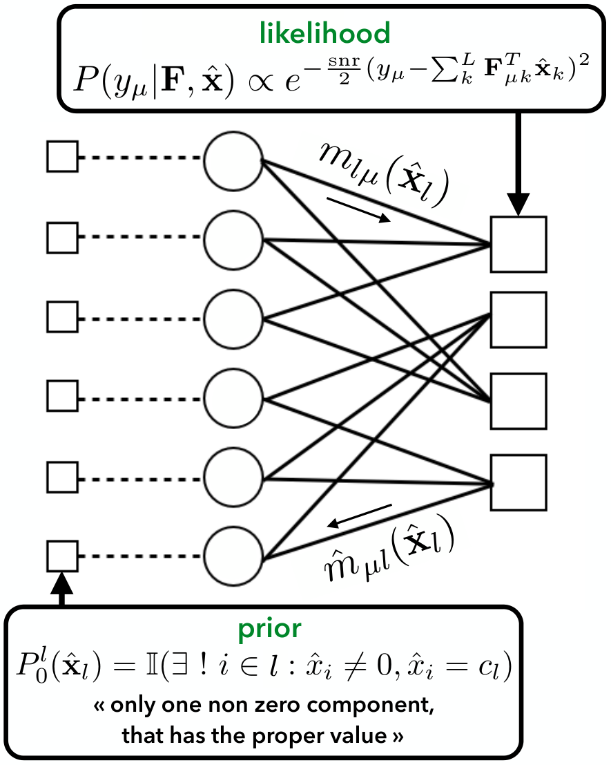
The purpose of AMP is to go beyond BP, in order to solve efficiently inference problems defined on dense graphs, which is here to compute the posterior marginal means of (4) for each section
| (10) |
It is a message-passing algorithm originally derived in its modern form for compressed sensing [18, 12, 11, 32] where one writes the BP equations on a densely connected factor graph with linear constraints ((8), (9) for sparse superposition codes), see Fig. 3 for the factor graph associated with (4). One then expands them up to the second order in the interaction terms, as we will derive it in appendix A. This step gives what is sometimes referred as the Gaussian approximation of BP, or the relaxed-BP algorithm [12]. A second step is then required to lower the number of messages, from which AMP is obtained. AMP can also be seen as a special case of the non-parametric BP algorithm [33] in the case where one takes only one Gaussian density per message in the parametrization, see [34] for details on this point.
In the AMP algorithm, even if the variables to infer are discrete, they are estimated using continuous representations. This is why when deriving AMP, we start from the BP equations (56), (57) written in the continuous framework. The marginals associated to the variables become densities. It is difficult to store these distributions if not properly parametrized. AMP being a second order Gaussian approximation of the original equations, these densities are Gaussian distributions simply parametrized by a mean and a variance. But other mean and variances of different quantities naturally appear in the derivation appendix A.
The final AMP decoder is given in Fig. 4. Let us give some meaning to the various quantities appearing. is an estimation of the codeword y at iteration , is its vector of associated variance per component (an estimation of how much AMP is “confident” in its estimate ). is the estimation of the message before the prior has been taken into account, which is thus the average with respect to the likelihood. are the associated variances. Finally and are the posterior estimate and variance of x, that takes into account all the information available at iteration . As such, should vanish in the successful decoding case. These are obtained thanks to the so-called denoisers and , given respectively by (79), (80).
In dense linear estimation with AWGN, when the noise variance and the prior are known (the prior is always known in the context of coding theory), this algorithm is Bayes-optimal and asymptotically performs minimum mean-square estimation as long as the communication rate is below the so-called BP threshold (or transition) , if it exists [12]. The transition location depends on the noise variance. This transition that prevents the algorithm to reach the MMSE estimate is inherent to the problem: we believe that its presence does not depend on the decoding algorithm. It can be, however, overcomed by a slight change in the code either by power allocation or by the use of spatial coupling that we present now (we shall see in sec.VI that the later solution seems to give better results in practice).
III-C Spatial coupling
We now discuss how the phase transition encountered by message-passing decoding is overcomed using spatially coupled codes. The term “spatially coupled codes” was first used in [9], in the context of LDPC codes. Their aim was to show that this “coupling” of graphs leads to a remarkable change in the algorithmic performances and that ensembles of codes designed in this way combine the property that they are capacity achieving under low complexity decoding, with the practical advantages of sparse graph codes: this is referred as threshold saturation11 1 Since the first version of this work, one of the authors have rigorously proven with his collaborators that this threshold saturation phenomenon indeed occurs for spatially coupled sparse superposition codes, and this whatever memoryless channel used for communication [35, 36].. Spatially coupled codes require, however, a very specific underlying graph, or in our case, a very specific coding matrix. Following these breakthrough, spatial coupling has been extensively used in the compressed sensing setting as well [10, 11, 12, 13, 15]. It rigorously allows to reach the information theoretical bound in LDPC [9] and in compressed sensing in the random i.i.d Gaussian measurement matrix case [13]. We thus naturally apply this technique here, using a properly designed coding operator: the sparse superposition codes scheme, being a structured compressed sensing problem, spatial coupling is expected to work.
In a nutshell, spatially coupled coding (or sensing) matrices are simply (almost) random band-diagonal matrices (see Fig. 5 for the general strucuture). More precisely, they represent a one dimensional chain of different systems that are “spatially coupled” across a finite window along the chain. A fundamental ingredient for spatial coupling to work is to introduce a seed at the boundary: the matrix is designed such that the first system on the chain lives into the “easy region” of the phase diagram, while the other ones stay in the “hard region”. Consider first a collection of different, independent sub-systems, where the first one has a low rate, so that a perfect decoding is easy, while all the other ones have a large rate where the naive decoder fail to reconstruct the message. In a spatially coupled matrix, additional measurements are coupling all these systems in a very specific way. Initially, we expect these couplings to be, at first, neglectible, so that the variables corresponding to the first system will be decoded, but not the other ones. As the algorithm is further iterated, however, the coupling from the first sub-system will help the algorithm to decode the second one, and so and so forth: this triggers a reconstruction wave starting from the seed and propagating inwards the signal. This is the basis of the construction in the LDPC case. Alternatively, one can also provide generic “statistical physics-type” argument on why these codes work (see [37, 38, 11, 39] for more on this subject)).
We study spatially coupled coding operators constructed as in Fig. 5, see the caption for the details. The operator has a block structure, i.e it is decomposed in blocks, each of them being either only zeros or a given sub-matrix. We focus on two particular constructions: the sub-matrices are made of random selections of modes of an Hadamard operator or are Gaussian i.i.d matrices. The Hadamard-based construction is predominantly used in this study for computational and memory efficiency purpose, and is presented in more details in the next section. In both cases, the matrix elements are always rescaled by some constant which enforces the power of the codeword to be one, so that the is the only relevant channel parameter.
We shall not prove in this paper that these coding matrices allow to reach threshold saturation (i.e that they allow to reach capacity under low complexity message-passing decoding) and let the study of this theorem for further work22 2 See the previous footnote., but we nevertheless conjecture that this is true. Indeed, we will show explicit examples where we construct codes that are going as close as needed to the desired threshold.
The structure of the coding operator induces a spatial structure in the signal, which becomes the concatenation of sub-parts . One has to be careful to ensure that these sub-parts remain large enough for the assumption behind AMP to be valid, essentially . Concurrently, however, the larger , the better it is to get closer to the optimal treshold. This is due to the relation (11) between the communication rate and the effective rate of the seed block and that of the remaining ones . Indeed, in the construction of Fig. 5, the link between the overall measurement rate defined in (1), that of the seed (the first block on the left upper corner on Fig. 5) and that of the bulk is
| (11) |
where can be asymptotically as large as the Bayes optimal rate. This optimal rate , defined precisely in sec.V, is the highest rate until which the superposition codes allow to decode (up to an inherent error floor) the input message for a given section size under MAP (or equivalently MMSE) decoding.
III-D The fast Hadamard-based coding operator
In order to get a practical decoder able to deal with very large messages, we combine the spatial coupling technique with the use of a structured Hadamard operator, i.e the standard fast Hadamard transform which is as efficient as the fast Fourier transform from the computational point of view. These operators have been empirically shown to be as efficient in terms of reconstruction error (or even better) as the random i.i.d Gaussian ones in the context of compressed sensing [24, 40, 41]. This is confirmed by the replica analysis for orthogonal operators done in [42].
All the blocks are thus constructed from the same Hadamard operator of size with the constraint that is a power of two, intrinsic to the Hadamard construction (simple numerical tricks such as -padding allow to relax this constraint at virtually no computational cost). The difference between blocks is the random selection of modes and their order, see Fig. 5.
The decoder requires four operators in order to work. We define , with , as the vector of size which is the block of e, itself of size . For example, in Fig. 5, the signal x is naturally decomposed as due to the block structure of the coding operator. We define similarly , with , as the vector of size which is the block of f, itself of size . We call the measurement rate of all the blocks at the block-row and from (11). In Fig. 5, and .

The notation (resp. ) means all the components of e that are in (resp. all the components of f that are in ). Using this, the operators required by the decoder are defined as following
| (12) |
In the case of an Hadamard-based operator, or depending on the non-zero block to which the indices belongs to. It implies that these four operators are implemented as fast transforms ( and ) or simple sums ( and ) and do not require any costly direct matrix multiplications. This is the advantage of using Hadamard-based operators: it reduces the cost of the matrix multiplications required by the decoder from (the cost with non structured matrices) to and the matrix has never to be stored in the memory, which allows to decode very large messages in a fast way without memory issues. The AMP decoder written in terms of these operators and that makes explicit the operator block structure is given in Fig. 4 [43, 24].
The practical implementation of the operator F requires caution: the necessary “structure killing” randomization of the Hadamard modes inside each non-zero block is obtained by applying a permutation of lines after the use of the standard fast Hadamard transform . For each block , we choose a random subset of modes . The definition of using is
| (13) |
where is the index of the block-row that includes , is the index of the first line of the block-row and is the component of . For instead,
| (14) |
where is the index of the block column that includes , is the index of the first column of the block column , is the standard Hadamard fast inverse operator of (which is actually itself) and is defined in the following way
| (15) |
Fig. 6 shows that when the signal sparsity increases, i.e when the section size increases, using Hadamard-based operators becomes equivalent to random i.i.d Gaussian ones in terms of performances (this point is studied in more details in [24]). We fix the and plot the distance in dB to the BP threshold (computed for ) at which the decoder starts to decode perfectly with Hadamard or random i.i.d Gaussian operators. Recall that is defined as the highest rate until which AMP decoding is optimal without the need of non constant power allocation nor spatial coupling. It appears that at low section size, it is advantageous to use random operators but as increases, structured operators quickly reach the random operator performances. The BP threshold is predicted by the state evolution analysis presented in the next section.
IV Results of the state evolution analysies
Most of the following empirical results are given for Hadamard-based operators for practical and computationnal reasons. In contrast, the state evolution analysies are derived (in appendix B) for i.i.d Gaussian matrices, which remains quite accurate when Hadamard-based operators are employed.
IV-A State evolution for homogeneous coding operators and constant power allocation
The state evolution technique (referred to as the cavity method in physics) is a statistical analysis that allows to monitor the AMP dynamics and performance in the limit of decoding infinitely large signals [18]. In the present case, we consider the matrix F to be i.i.d Gausian with zero mean, for which state evolution has been originally derived [18]. Extension to more general ensembles such as row-orthogonal matrices could be considered [42] but it is out of the scope of the present paper. In addition, the present authors have numerically shown in [24] that the state evolution analysis derived in the Gaussian i.i.d case is a good predictive tool of the behavior of the AMP decoder with structured operators such as the Hadamard one, despite not perfect nor rigorous.
The complete (but heuristic) derivation of the state evolution recursions is done in appendix B-B. We define
| (16) |
as the asymptotic average (7) per section of the AMP estimate at iteration , where the average is over the model (2). The state evolution should be initialized with initial condition , corresponding to no prior knowledge of the sent message. A convenient form of the state evolution recursion is
| (17) | ||||
| (18) |
where is a -d unit centered Gaussian measure, and the following functions are used
| (19) | ||||
| (20) |
The interpretation of is the following: it is the MMSE associated with the estimation of a single section sent through an effective AWGN channel with noise variance , where z plays the role of this effective AWGN. Here outputs the asymptotic estimate by the AMP decoder of the posterior probability that the component is the unique in the section, given that is is actually the in the transmitted section (all section permutations are equivalent). Instead, outputs the asymptotic posterior probability estimate by the AMP decoder that the component is the given that is is actually the component that is the true , thus of an error. With this interpretation in mind, there is a simple correspondance between the and the given by
| (21) |
From this equation, we can predict the asymptotic time evolution of the decoder performance measured by the , such as in Fig. 7. Recall that the state evolution predictions are asymptotically exact when AMP is used with i.i.d Gaussian coding matrices, and approximate but yet accurate for Hadamard operators. The black curves on this figure represent the iteration of (17), (18), (21) for different parameters and fixed section size , using randomized Hadamard-based or random Gaussian i.i.d operators. (21) and (17) are computed at each step by monte carlo.
We restrict these experiments to relatively low values of , because if these are too high, the experimental and theoretical curves would stop at some iteration without reaching an error floor and decoding “seems” perfect. For the experimental curves, this is due to the fact that in order to observe an , the message must be at least made of sections, which is not the case for messages of reasonnable sizes when the asymptotic is very small. In fact, when the rate is below the BP threshold, the decoding is usually perfect and is found to reach with high probability . The black theoretical curves should anyway always reach a positive error floor but they would not because of the same reason: this error floor is so low at high that the minimal sample size required to observe it when computing the integrals present in (17), (21) by monte carlo should be way too large to practically deal with.
We also naturally observe, from the definition of the state evolution technique as an asymptotic analysis, that the theoretical and experimental results match better for larger messages. At rate (the curves converging to an high for the first two cases on Fig. 7), we see that AMP decoding does not reconstruct the messages and converges to an error precisely predicted by the state evolution. On the contrary, below the threshold, the reconstruction succeeds up to an error floor dependent on the parameters . We also observe, as in [24], that the state evolution, despite being derived for random i.i.d Gaussian matrices, predicts well the behavior of AMP with Hadamard-based operators, especially for large .
Let us discuss a bit more the error floor. The replica analysis from which we borrow some results now will be discussed in details in sec.V, but let us just consider now the potential (28) obtained from this analysis as a function which extrema correspond to the fixed points of the state evolution (17).
In sparse superposition codes, there exists a inherent error floor, and this independently of the finite size effects. Indeed, for any finite section size , the asymptotic state evolution and replica analysies show that this error floor is present, but is in general very small and quickly decreasing when or the increase. See for example the Fig. 13, obtained from the replica analysis, that shows how the SER associated with the MMSE estimator (i.e the optimal ) of sparse superposition codes with constant power allocation falls with a power law decay as a function of or the . The right part of Fig. 10 also illustrates the error floor decaying when the increases. It shows the potential function, which maxima indicate the stable fixed points of the state evolution, at fixed , and for values of the (the top black curve is for , the bottom one for ). On each curve, there is a red point at a relatively low value, which corresponds to the MMSE of the code (as long as , otherwise the MMSE corresponds to the high error maximum). This is the error floor.
This phenomenology is also present in low density generator matrix (LDGM) codes. These codes also present an error floor, but a very important difference between sparse superpostion codes and LDGM ones is that for sparse superposition codes, the error floor can be made arbitrarily small for a fixed by increasing while maintaining low-complexity AMP decoding. Indeed, in the case of an i.i.d Gaussian operator (spatially coupled or not), the decoding complexity of AMP scales as , or with Hadamard-based operators. In the case of LDGM codes, the error floor can be decreased as well by increasing the generator matrix density, but it has a large computational cost: the BP decoder used for LDGM codes which is very similar to the one used for LDPC codes [7] has to perform a number of operations which scales exponentially with the average degree of the factor nodes in the graph. Thus the reduction of the error floor in LDGM codes becomes quickly intractable due to this computational barrier that is not present in sparse superposition codes, where the cost is at worst quadratic with the section size .
Finally let us stress that the rapid decrease of the error floor observed in Fig. 13 when the increases is a generic scenario, in the sense that the very same phenomenon happens when increases or the rate decreases. This can be easily understood. Looking at the state evolution recursion for the effective noise variance (18) together with (17) and the functions (19), (20), wee observe the following: it is perfectly equivalent to decrease the rate or increase by the proper amount, and increasing the has a similar effect to reduce the effective noise variance (but not in a simple multiplicative way as and ).
IV-B State evolution for spatially coupled coding operators and constant power allocation
In the spatially coupled case, the interpretation of state evolution is similar to the homogeneous operator case: tracks the asymptotic average of the AMP decoder in the block of the reconstructed signal, see Fig. 5. It is further interpreted as the MMSE associated with an effective AWGN channel which noise variance (23) now depends on the block index, and which is coupled to the other blocks. The derivation of the analysis for the spatially coupled operators is presented in details in appendix B-C. The final recursion for the average asymptotically attained by AMP for the block is
| (22) | ||||
| (23) |
where the functions are given by (19), (20). The relation linking the and is similar to the homogenous operator case
| (24) |
Fig. 8 shows a comparison of predicted by state evolution (black curves) with the actual reconstruction per block of messages transmitted using sparse superposition codes with Hadamard-based spatially coupled operators and AMP. Again, the discrepancies between the theoretical and experimental curves come from that state evolution is derived for random i.i.d Gaussian matrices. The final error using these Hadamard operators is at least as good as predicted by state evolution. As already noted in the homogeneous case and [24], AMP in conjunction with structured Hadamard-based operators converges slightly faster to the predicted final error than Gaussian matrices.
IV-C State evolution for homogeneous coding operators and non constant power allocation
From the previous analysis sec.IV-B, we can trivially extract the state evolution for sparse superposition codes with non constant power allocation when an homogeneous i.i.d Gaussian matrix is used. This is done thanks to the transformation of Fig. 9: starting from an homogeneous matrix and non constant power allocated message, we convert the system into an equivalent one (from the state evolution point of view) that has a structured matrix but with a constant power allocated message.
Let us detail the procedure. Suppose the message is decomposed into groups, where inside the group , the power allocation is the same for all the sections belonging to this group and equals . Now one must create a structured operator starting from the original one, decomposing it into column blocks and multiply all the elements of the column block by , as shown in Fig. 9. This new operator acting on a constant power allocated message is totally equivalent to the original system from the state evolution point of view, and fortunately, we already have the state evolution for this new system from the previous section. Using (23) in the present setting, one has to be careful with the value of defined as the number of lines over the number of columns of the block-row. Here there is a unique value that equals where is the measurement rate of model (1). Given that, we obtain for all
| (25) | ||||
| (26) |
V Results of the replica analysis
V-A The replica symmetric potential of sparse superposition codes with constant power allocation
The replica analysis is an heuristic asymptotic and static statistical analysis (as opposed to the dynamical state evolution analysis). It allows to compute the so-called replica symmetric free entropy (28), a potential function of the . This potential is related to the mutual information (per section) of model (2) between the random received corrupted codeword and the radom transmitted message through
| (27) |
This potential contains all the information about the location of the information theoretic and algorithmic transition (blocking the decoder if and no spatial coupling is employed) of the problem, the MMSE performance or the attainable asymptotic of AMP [23]. Indeed, AMP is deeply linked to : recall that the extrema of this potential (28) match the fixed points of state evolution (17), (18).
The replica method used to derive this potential has been developed in the context of statistical physics of disordered systems in order to compute averages with respect to some source of quenched disorder of physical observables of the system, the and in the present case. The method has then be extended to information theoretical problems [44, 45] due to the close connections between the physics of spin glasses and communications problems [27, 45], where the sources of quenched disorder to average over are the noise, coding matrix and the transmitted message realizations. See the recent rigorous results on the validity of the replica approach for linear estimation [23, 22].
The expression of the potential for sparse superposition codes at fixed section size with constant power allocation is
| (28) |
where
| (29) |
This potential depends on that is interpreted as a mean-square error per section, but it can be implicitely expressed as a function of the section error rate thanks to the one-to-one correspondance (21) between the and .
We plot (28) in the case on Fig. 10. The AMP algorithm follows a dynamics that can be interpreted as a gradient ascent of this potential, which starts the ascent from an high error (i.e from a random guess of the message). The brown curve of the left figure thus corresponds to an “easy” case as the global maximum is unique and correponds to a low error, which is the optimal , i.e associated to the MMSE through (21) (the optimal is the error associated with the global maximum of this potential). There and AMP is asymptotically optimal in the sense that it performs MMSE estimation (and thus leads to optimal ). The green curve corresponds to the BP threshold, that is the appearance of the first horizontal inflexion point in when increasing . This threshold marks the appearance of the hard phase, where the inference is typically hard and AMP cannot decode (without spatial coupling or power allocation). The local maximum at high error blocks the convergence of AMP, preventing it to reach the MMSE. Still, the MMSE corresponds to an higher free entropy meaning that it has an exponentially larger statistical weight (and thus corresponds to the true equilibrium state in physics terms). The problem is to reach it under AMP decoding despite the precense of the high error local maximum. Spatial coupling has been specifically designed to achieve this goal. The pink curve (or blue and red ones for other ) marks the appearance of the impossible inference phase defined as the rate where the low and high error maxima have same free entropy. At this threshold, the local and global maxima swith roles which corresponds to a jump discontinuity of the MMSE and optimal from low values to high ones (one speaks in this case of a first order phase transition). In this phase, even optimal MMSE estimation leads to a wrong decoding. In constrast, if , the AMP algorithm combined with spatial coupling or well designed power allocation is theoretically able to decode and as we will see, tends to the Shannon capacity as , see sec.V-D and sec.VI.
V-B Results from the replica analysis for sparse superposition codes with constant power allocation and finite section size
From this analysis, we can extract the phase diagram of the superposition codes scheme. Fig. 11 shows phase diagrams for different values, where the axis is the section size while the axis is the distance to the Shannon capacity in dB. The blue curve is the BP threshold extracted from the potential (28) which marks the end of optimality of the AMP decoder without spatial coupling or proper power allocation. The red curve is the optimal threshold: the highest rate until decoding is information theoretically possible33 3 also formally defined as the first non-analiticity point of the asymptotic mutual information (27) when increasing , see [23]., also extracted from (28). The black dashed curve is the asymptotic BP threshold (40), which derivation is done in sec. V-C.
A first observation is that the BP threshold is converging quite slowly to its asymptotic value (40) (computed in the next section) if compared to the convergence rate of the optimal threshold to the capacity. We also note that the section size where start the transitions, and thus marks the appearance of the hard phase where the AMP decoder without spatial coupling is not Bayes optimal anymore, increases as the decreases. When the is not too large, we see that the optimal and BP thresholds almost coincide at small values, such as for at and for . Below this section size value, there are no more sharp phase transitions as only one maximum exists in the potential (28) and the AMP dedoder is optimal at any rate even without spatial coupling. In this regime, the increases continuously with the rate. As the increases, the curves split sooner until they remain different for all such as in the case. See Fig. 14 and Fig. 13 for more details on the achievable values of the . A second observation is that despite the optimal performance of the code improves and approaches capacity with increasing , instead the AMP perfomance monotonously reduces (in terms of possible communication rate). But as we will see with Fig. 16 and Fig. 17, spatial coupling allows to enter the hard phase (between the two transitions), making AMP to improve as well with increasing .
Fig. 12 gives details on the rate of convergence of the thresholds to their asymptotic value, and it seems it can be well approximated by a power law in both cases. On Fig. 12 we show the differences between the finite transitions of Fig. 11 and their asymptotic (in ) values which are the capacity for the optimal threshold (as shown in the previous subsection) and (40) for the BP threshold. It appears that the scaling exponents increase in amplitude as the increases: the larger the , the faster the convergence to asymptotics values is.
Fig. 13 represents how the optimal , the corresponding to the MMSE, evolves with the section size at fixed rate and (left plot) and then as a function of the at fixed rate and (right plot). In both cases, the curves seem to be well approximated by power laws with exponent given on the plots. The points are extracted from the potential (28).
Fig. 14 quantifies the optimal performance of the code, obtained from the state evolution analysis. We plot the base 10 logarithm of the corresponding to the maximum of the potential (28) that has lower error, this as a function of and (again the state evolution and replica analysies are equivalent as shown in appendix C-B). For high noise regimes, the plotted is always attainable by AMP without the need of spatial coupling as there is no sharp phase transition (the potential has a single maximum). For lower noise regimes, the plotted matches the optimal one as long as (pink curves). When there is no transition (before the pink curves start), the is the optimal one too (here also, the potential has a single maximum). Fig. 13 left plot is a cut in the plot. The information brought by the replica analysis, not explicitly included in the state evolution analysis, is the identification of the phase in which the system is (easy/hard/impossible inference) for a given set of parameters .
V-C Large section limit for sparse superposition codes with constant power allocation
In order to access the limit of the potential and thus the asymptotic performance of the code, we need to compute the asymptotic value of the integral that appears in the potential (28):
| (30) |
Recall is an standardized Gaussian measure over the i.i.d . We present here an heuristic computation based on an analogy with the so-called random energy model [46, 27] of statistical physics. An alternative heuristic derivation of the following results based instead on the replica method is given in appendix C-C. This independent analysis brings the same results, strenghtening the claim of the exactness of the analysis despite not being rigorous.
We shall drop the dependency of (29) in to avoid confusions. We adopt here the vocabulary of statistical physics [27]: this is formally a problem of computing the average of the logarithm of a partition function of a system with (disordered) states. Indeed, one can rewrite (30) as:
| (31) | ||||
| (32) |
where
| (33) | ||||
| (34) |
In fact is formally known as a random energy model in the statistical physics literature [46, 27], a statistical physics model where i.i.d energy levels are drawn from some given distribution. This analogy can be further refined by writing the energy levels as and by denoting as the temperature. In this case, a standard result [46, 27, 47] is:
- •
The asymptotic limit for large of exists, and is concentrated (i.e it does not depend on the disorder realization, that is the ensemble of energy levels).
- •
It is equal to .
We can thus now obtain the value of the integral by comparing and and keeping only the dominant term. First let us consider the case where :
| (35) |
where the approximate equality is an ansatz motivated by physical arguments: at high temperature, all the configurations have approximately same weight and thus the favored state has negligible influence. In communication terms, plays the role of the variance of an effective AWGN added to the transmitted section and thus when it is high, it prevents recovering the section. If, however, , then using again an ansatz one obtains
| (36) |
Indeed, at low temperature, the favored state should be dominant. In communication terms, the noise is low and thus one recovers the section. From (32) this leads to
| (37) |
From these results combined with (28), we now can give the asymptotic expression of the potential:
| (38) |
with , see (129). See Fig. 15 for a graphical representation of this potential.


Let us now look at the extrema of this potential. We see that we have to distinghish between the high error case ( so that ) and the low error one (, so that ).
In the high error case, the derivative of the potential is zero when
| (39) |
which happens when . Therefore, if both the condition and are met, there is a stable extremum (a maximum) of the potential at . The existence of this high-error maximum thus requires , and we thus define the asymptotic critical rate beyond which the state at is stable:
| (40) |
Since we initialize the recursion at when we attempt to reconstruct the signal with AMP, we see that is a crucial limit for the reconstruction abality by message-passing. See the right part of Fig. 15 for an illustration of how this transition is separated from the Shannon capacity, leading to a computational gap that may be closed by spatial coupling.
In the low error case, the derivative of the potential is zero when:
| (41) |
which happens when . Hence, there is another maximum with zero error. Let us determine which of these two is the global one. We have
| (42) | ||||
| (43) |
so that the two are equal when , or equivalently when , where we recognize the expression of the Shannon Capacity for the AWGN. These results are confirming that, at large value of , the optimal value of the section error rate vanishes. Therefore perfect reconstruction is possible, at least as long as as the rate remains below the Shannon capacity after which, of course, this could not be true anymore. This confirms the results by [2, 3] that these codes are capacity achieving.
These results are summarized by Fig. 15. The analysis of have shown that the only possible maxima are at and , which implies that the error floor vanishes as increases. We have shown that if , then has a unique maximum at , meaning that AMP is optimal and leads to perfect decoding. Otherwise two minima coexist and AMP is sub-optimal. In this regime it is required to use spatial coupling or power allocation.
V-D Optimality of the AMP decoder with a proper power allocation
In this section, we shall discuss a particular power allocation that allows AMP to be capacity achieving in the large size limit, without the need for spatial coupling. We shall work again in the large section size limit.
We first divide the signal into blocks, see Fig. 9. For our analysis, each of these blocks has to be large enough and contains many sections, each of these sections being itself large so that , where is the number of sections per group. Now, in each of these blocks, we use a different power allocation: the non-zero values of the sections inside block are all equal to . This is precisly the case which we have studied in sec. IV-C, so we can apply the corresponding state evolution in a straightforward manner.
Our claim is that we can use the following power allocation:
| (44) |
where is the Shannon capacity. We choose such that the power of the signal equals one, so that . With this definition, we have
| (45) |
This leads to the following useful identity:
| (46) |
Now, we want to show that, if we have decoded all sections until the section , then we will be able to decode section as well. If we can show this, then starting from we will have a succession of decoding until all is decoded, and we would have shown that this power allocation works. In this situation, using (26) and the expression of the rate (1), we have for the section that
| (47) |
with
| (48) |
where we have used our assumption of having already decoded until included: . (48) is the average per section if all has been decoded until , given that the initial is and that we have to remove what has been already decoded. We now ask if the block can be decoded as well. The evolution of the error in this block is given by (25), and we have seen, in sec. V-C, that the condition for a perfect decoding in the large limit is simply that . Using (47), we thus need the following to be satisfied (as long as ):
| (49) |
If this condition is satisfied, there is no BP threshold to block the AMP reconstruction in the block , and thus the decoder will move to the next block, etc. We thus need this condition to be correct . Let us perform the large limit (remembering that stays however finite). We have from (44) and (45) that
| (50) | ||||
| (51) |
Now, we note from the expression of the Shannon capacity that the can be written as
| (52) |
so using (46), (48) it leads to
| (53) |
Therefore to leading order, we have using (51) that
| (54) |
so that the condition (49) becomes for large
| (55) |
or equivalently . This shows that, with a proper power allocation (44) and as long as , there aymptotically cannot exist a local maximum in the potential; or equivalently, that the AMP decoder cannot be stuck in such a spurious maximum and will reach the optimal solution with perfect reconstruction .
VI Numerical experiments for finite size signals
We now present a number of numerical experiments testing the performance and behavior of the AMP decoder in different practical scenarios with finite size signals. The first experiment Fig. 16 quantifies the influence of the finite size effects over the superposition codes scheme with spatially coupled Hadamard-based operators, decoded by AMP. For each plot, we fix the and the alphabet size and repeat decoding experiments with each time a different signal and operator drawn from the ensemble . The curves present the empirical block error rate (blue and yellow curves) which is the fraction of instances that have not been perfectly decoded (i.e such that the final ) end the (red and purple curves). This is done for two different sizes and . When the curves stop, it means that the empirical block error rate (and thus the section error rate as well) is actually . The dashed lines are the BP threshold and optimal threshold extracted respectively from the state evolution analysis and potential (28) and the solid black line is the capacity . Thanks to the fact that at large enough section size , the gap between the BP threshold and capacity is consequent, it leaves room for the spatially coupled ensemble with AMP decoding to beat the transition, allowing to decode at as in LDPC codes. For small section size , the gap is too small to get real improvement over the full operators. We also note the previsible fact that as the signal size increases, the results are improving: one can decode closer to the asymptotic transitions and reach a lower error floor. For , the sharp phase transition between the phases where decoding is possible/impossible by AMP with spatial coupling is clear and gets sharper as increases.
The next experiment Fig. 17 is the phase diagram for superposition codes at fixed like on Fig. 11 but where we added on top finite size results. The asymptotic rates that can be reached are shown as a function of (blue line for the BP threshold, red one for the optimal rate). The solid black line is the capacity. Comparing the black and yellow curves, it is clear that even without spatial coupling, AMP outperforms the iterative successive decoder of [2] for practical values. With the Hadamard-based spatially coupled operators and the AMP decoder, this is true for any and is even more pronounced (brown curve). The green (resp. pink) curve shows that the homogeneous (resp. spatially coupled) Hadamard-based operator has very good performances for reasonably large signals, corresponding here to a blocklength (the blocklength is the size of the transmitted vector ).
Finally, the last experiment Fig. 18 is a comparison of the efficiency of the AMP decoder combined with spatial coupling or an optimized power allocation. The optimized power allocation used here comes from [21]. We repeated their experiments and compared the results to a spatial coupling strategy. Comparing the results with Hadamard-based operators, given by the red and yellow curves for power allocation and spatial coupling respectively, it is clear that spatial coupling (despite not being optimized for each rate) greatly outperforms a (per rate) optimized power allocation scheme.
In addition, we see that our red curve corresponding to the optimized power allocation homogeneously outperforms the blue curve of [21] with exactly the same parameters. As we have numerically shown that Hadamard-based operators gets same final performances as Gaussian i.i.d ones as used in [21] (see [24] and Fig. 6), the difference in performance must come from the AMP implementation: in our decoder implementation (that we denote by on-line decoder), there is no need of pre-processing but in the decoder of [21] (denoted by off-line), quantities need to be computed by state evolution before running.
The advantage of spatial coupling (yellow) over power allocation (red) is independent of the AMP decoder implementation and the fact that we use Hadamard-based operators, as it outperforms the red curve obtained with our on-line decoder and Hadamard-based operators as well. This is true at any rate except at very high values where spatial coupling does not allow to decode at all, while the very first components of the signal are decoded using power allocation as their power is very large. But it is not a really useful regime as only a small part of the signal is decoded anyway, even with power allocation. The green points show that a mixed strategy of spatial coupling with optimized power allocation does not perform well compared to individual strategies. This is easily understood from the Fig. 9: a power allocation modify the spatial coupling and worsen its original design. In addition we notice that at low rates, a power allocation strategy performs worst that constant power allocation without spatial coupling (purple curve).
VII Conclusion and future works
We have derived and studied the approximate message-passing decoder, combined with spatial coupling or power allocation, for the sparse superposition codes over the additive white Gaussian noise channel. Clear links have been established between the present problem and compressed sensing with structured sparsity.
On the theoretical side, we have computed the potential of the scheme thanks to the heuristic replica method and have shown that the code is capacity achieving under AMP decoding in a proper limit. The analysis shows that there exists a sharp phase transition blocking the decoding by message-passing before the capacity. The analysis also shows that the optimal Bayesian limit, that can be reached by AMP combined with spatial coupling or power allocation, tends to the Shannon capacity as the section size (i.e the input alphabet size) increases. We have also derived the state evolution recursions associated to the AMP decoder, with or without spatial coupling and power allocation. The replica and state evolution analysies have been shown to be perfectly equivalent for predicting the various phase transitions as the state evolution can be derived as fixed point equations of the replica potential. The optimal asymptotic performances have been studied and it appeared that the error floor decay and the rates of convergence of the various transitions to their asymptotic values (in the section size) empirically follow power laws.
On the more practical and experimental side, we have presented an efficient and capacity achieving solver based on spatially coupled fast Hadamard-based operators. It allows to deal with very large instances and performs as well as random coding operators. Intensive numerical experiments show that a well designed spatial coupling performs way better than an optimized power allocation of the signal, both in terms of reconstruction error and robustness to noise. Finite size performances of the decoder under spatial coupling have been studied and it appeared that even for small signals, spatial coupling allows to obtain very good perfomances. In addition, we have shown that the AMP decoder (even without spatial coupling) beats the iterative succesive decoder of Barron and Joseph for any manageable size. Futhermore, its performances with spatial coupling are way better for any section size.
The scheme should be now compared in a systematic way to other state-of-the-art error correction schemes over the additive white Gaussian noise channel. On the application side, from the structure of the reconstructed signal itself in superpostion codes, we can also interpret the problem as a structured group testing problem where one is looking for the only individual that has some property (for example infected) in each group. Finally, the link with the random energy model and the similarity of sparse superposition codes with Shannon’s random code suggest that these codes should be capacity achieving for a much larger class of channels. We plan to look at these questions in future works44 4 Since the publication of the first version of this paper, one of the author has extended the study of sparse superposition codes and have shown that this code achieves capacity on any memoryless channel with spatial coupling and under generalized approximate message-passing decoding, see [36]..
Appendix A Derivation of the approximate message-passing decoder from belief-propagation
The following generic derivation is very close to that of [12] albeit in the present case it is done in a framework where the variables for which we know the prior are -d (the sections) instead of the -d ones (for which we want to derive closed equations). For readibility purpose, we drop the time index from the equations and add it back at the end.
A-A Gaussian approximation of belief-propagation for dense linear estimation: relaxed belief-propagation
It starts from the usual loopy BP equations. We write them in the continuous framework despite the variables we want to infer are discrete. In this way the messages are densities, that can be expanded later on, an essential step in the derivation. Recall that is the vector of entries of the row of the matrix F that act on , see Fig. 2. Furthermore, vectors are column vectors and thus terms of the form for some a are scalar products. Then BP reads
| (56) | ||||
| (57) |
where and we write with some abuse of notation to refer to the set of indices of the scalar signal components composing the section. is the prior (6) that strongly correlates the components inside the same section by enforcing that there is a single non-zero in it, with value given by the power allocation.
These intractable equations must be simplified. Recall that we fix the power to which implies a scaling for the coding matrix i.i.d entries. Thus as which allows to expand the previous equations. We will need the following transform . Using this for , we express (56) as
| (58) |
In order to define the approximate messages using a Gaussian parametrization (that is using the first and second moments), we need the following vector definitions
| (59) |
where represents a generic index and the square operation is componentwise. Expanding (58), keeping only the terms not smaller than and approximating the result by an exponential we obtain
| (60) |
The symbol means equality up to terms of lower order than . The Gaussian integration with respect to can now be performed. Putting all the -independent terms in the normalization constant , we obtain
| (61) | ||||
| (62) |
where we introduced the shorthand notations
| (63) |
It is noteworthy that at this stage, the joint distribution of the signal components inside the section is a multivariate Gaussian distribution with diagonal covariance. The independence of in the measure is not an assumption, and it arises in the computation as from the fact that the entries of the coding matrix F are independently drawn, which makes the non diagonal terms of the covariance of a smaller order than the diagonal ones. We can thus safely neglect them as . This decouples in the factor-to-node messages all the components inside the same section, which simplifies a lot the equations. The strong correlations between the signal components inside a same section are purely due to the prior (6), and will be taken into account in the next step. Plugging (61) in (57), we deduce the node-to-factor messages
| (64) | ||||
| (65) |
Here sums of the form are vectors of size and the inverse operation for a vector is a componentwise operation, similarly as . Each message is now expressed as a Gaussian distribution, fully parametrized by its first and second moment. Thus the algorithm can be expressed only with these moments, instead of the messages.
We define as the section index to which the component belongs to. Depending on the context that should be clear, it may also be the set of indices of the components of the section to which belongs component . We now introduce a generic probability measure for a section. It is a joint probability distribution over the components composing a given section.
| (66) |
Here is a normalization. We define the denoisers as the marginal mean and variance with respect to the measure of the signal component
| (67) | ||||
| (68) |
where the notation means presently that the component of the vector associated to the component of the signal is selected, where . For example in (67), x is the -d vector of marginal means with respect to the measure . The denoisers are thus taking -d vectors as input and output a single scalar. The interpretation of these functions is the following. The so-called “AMP fields” which are the mean and variance of the signal component with respect to the likelihood at a given time are computed. These quantities summarize the overall influence of the other variables on the one. Then in order to estimate the posterior marginal mean and associated variance, the prior has to be taken into account. This is the role of the denoisers to do so. One may also interpret the denoiser as the MMSE estimator associated with an effective AWGN channel of noise variance and channel observation .
Now note that the marginal (66) appearing in the denoisers definitions verifies given by (64). Then the Gaussian approximation of the BP equations is
| (69) |
At this stage, after indexing with the time, the algorithm defined by the set of equations (62), (63), (65), (69) together with the definition of the denoisers is usually referred to as relaxed-BP [11]. After convergence, the final posterior estimates and variances of the signal components are obtained from
| (70) | ||||
| (71) |
In compressive sensing and more generally for linear estimation problems with AWGN and defined on dense factor graphs, this algorithm is asymptotically exact (as the number of sections ) in the sense that it is perfectly equivalent to the BP algorithm. This means that the two algorithms would provide the same estimation of the signal up to corrections that asymptotically vanish. This equivalence is a direct consequence of the fact that the coding matrix has i.i.d entries and is dense. With this in mind, from “central-limit like arguments”, the Gaussian expansions that we have introduced are very natural and asymptotically well justified.
A-B Reducing the number of messages: the approximate message-passing algorithm
We can simplify further the equations, going from the relaxed-BP algorithm with messages ( per edges on the factor graph Fig. 3) to the AMP algorithm where only messages are computed. The following expansion is called the Thouless-Anderson-Palmer (TAP) equations in statistical physics [27], which is again exact in the same sense as before: the estimation provided by AMP is asymptotically the same as the BP one in the limit .
Deriving AMP starts by noticing that in the limit (and thus the number of factors diverges as well, while the ratio is kept fixed), the quantities (65), (69) become almost independent of the index . This is equivalent to say that each factor’s influence becomes infinitely weak as there are so many. We can thus rewrite (65), (69) as marginal quantities, i.e that depend on a single index (as opposed to the cavity quantities that depend on both a variable and factor indices, i.e an edge index), while keeping the proper first order corrections in . These correcting terms, called the Onsager reaction terms in statistical physics [27, 12], are essential for the performance of AMP and they make the resulting AMP algorithm different with respect to a naive mean-field approach [48].
Recall that all the operations such as or the dot product applied to vectors or matrices are componentwise, whereas is the usual inner product between vectors. Furthermore, keep in mind that we always consider the section size finite as for the derivation, so that if terms of order are summed, the result remains of order . The aim now is to compute the corrections of the cavity quantities around their associated marginal approximation. Let us start with the corrections to the posterior average given by (69). Denoting (and similarly for ), we obtain
| (72) |
Now we use the fact that is a strictly positive term and can be of both signs, see (62), thus and are both . After some algebra, we obtain the first order corrections to and similarly, the corrections to as well
| (73) |
where are defined by (70). We introduced , the vector of corrections linking the cavity quantity to the marginal one , and similarly for . Their components can be of both signs. To go further, we thus need to express in function of marginal quantities only. Keeping only the dominant terms, we obtain
| (74) | ||||
| (75) |
As these quantities depend on (63) that depend themselves on cavity quantities, we need to expand them as well. Using (73), we obtain
| (76) | ||||
| (77) |
The last equality is obtained neglecting terms and combining the relation
| (78) |
with (73) and (62). We thus now have a closed set of coupled equations on the marginal quantities . Adding back the time index to these equations to get an iterative algorithm, we obtain the AMP algorithm of Fig. 4.
A-C Taking into account the prior for sparse superposition codes
The only problem-dependent objects in AMP are the denoisers given by (67), (68) that both depend on the prior (6). Let us derive them for any power allocation . Using (6), we obtain after simple algebra the posterior estimate and variance at time
| (79) | ||||
| (80) |
where are the AMP fields of the section , to which the component of the signal belongs to. This closes the derivation of the AMP decoder for sparse superposition codes.
A-D Further simplifications for random matrices with zero mean and homogeneous variance
We can go further in the simplification of some quantities computed by the decoder Fig. 4 by considering the elements equal to their variance. We start considering the general case where the matrix can have a block structure encoded through the variance matrix , and thus we assume , see Fig 5 (the factor makes the codeword fluctuations of , such that the power has proper scaling. Note that in order to have a codeword power strictly equal to one, the matrix elements are also multiplied by a proper constant). Here the notation () means the block index (resp. ) to which the factor index (resp. component ) belongs to.
This step is justified by the fact that the average with respect to the coding matrices ensemble of all the objects appearing in the decoder that depend on such squared elements (such as ) are whilst their variance are , see [12]. Thus in the large signal limit, we can neglect their fluctuations by simply replacing the matrix squared elements by their variance. Considering the most general version of AMP (the left version of Fig. 4) where it is written in terms of the operators, the dependency is just in the and operators that now depend only on the block indices and can thus be approximated as
| (81) |
Thanks to this simplification, we obtain the simpler decoder of Fig. 19. It is asymptotically equivalent to AMP as it provides the same estimation when and for matrices which have zero mean entries with homogeneous variance per block .
Let us show how to go from this simplified AMP decoder to the equivalent notations of [17] in the case of a fully homogeneous matrix, i.e that does not have a block structure. We start defining the residual
| (82) | ||||
| (83) |
Then plugging the expression of Fig. 19 into the denoiser, one obtains
| (84) |
It is naturally considered that the blocks are such that all the components inside a same section are part of the same block. We define the shorthand notations
| (85) |
Now using the definition of where is a vector full of ones of size , we obtain
| (86) |
where we have used the property (78) of the denoising function for the last equality. (83), (84) and (86) together with the iteration of from Fig. 19 forms a set of closed equations, which is just AMP written in term of the residual. We now show that this form gives back the one of [17] in the full operator case, i.e when . In this case, the quantities in the algorithm become
| (87) | ||||
| (88) |
| (90) | ||||
| (91) | ||||
| (92) |
using (87), (88) for the last equality. The last step is to rescale the coding matrix by dividing its elements by , that implies that the codeword is similarly rescaled. We finally obtain the more classical form of AMP for homogeneous matrices
| (93) | ||||
| (94) | ||||
| (95) |
where is the rescaled residual, and
| (96) | ||||
| (97) |
Appendix B State evolution analysis
We consider for the present analysis that the matrix F has i.i.d Gausian entries with zero mean and a variance scaling as , such that the codeword has fluctuations (and thus a power) of .
B-A The Bayesian optimal setting and the Nishimori identity
Before deriving the state evolution analysis, let us show how the perfect knowledge of the statistical properties of the communication channel and of the signal prior imply great simplifications and useful identities for the state evolution and replica analysies. This perfect knowledge of all the problem parameters is refered as the Bayesian optimal setting. The induced simplifications are refered as the Nishimori identities in statistical physics [12, 27]. While these were first derived as a concequence of a gauge symmetry in spin systems [45], they are actually a direct concequences of Bayes rule in the present continuous framework. We shall here derive the Nishimori identities similarly to [12].
Assume the signal x is distributed according to some known prior and its observation y is drawn from some known conditional distribution . Furthermore, assume drawn from the posterior . Then for any function , and using the Bayes formula, we obtain the following relation
| (98) |
We have renamed to emphasize that is drawn from the posterior (independently of ) and thus play the same role as : we speak about two “replicas”. The Nishimori identity (98) says that if a function depending on both the signal and a replica is averaged with respect to both the quenched disorder and the posterior, then one may replace in it the signal by a new i.i.d replica distributed according to the posterior (the two replicas being distributed according to the product measure). In particular, this implies
| (99) |
In statistical physics, macroscopic intensive observables (i.e divided by the system size), such as the MMSE or in the present setting, are assumed to concentrate around their expectation with respect to the problem realization (that is with respect to the posterior and quenched disorder) as the system size diverges. This assumption implies that we can replace the asymptotic value of such observables by their expectation55 5 See for example [49] for such concentration proofs..
Let us use this concentration assumption combined with the Nishimori identity to show a number of useful sub-identities. Define the following overlaps
| (100) |
where are i.i.d replicas distributed according to (4). Recall that is the MMSE estimate (10). The concentration of these overlaps together with the Nishimori identity straightforwardly implies that in the limit
| (101) | ||||
| (102) |
where the last equality is valid for sparse superposition codes.
These identities imply various expressions of the MMSE . Let us show that it equal to the posterior variance of the MMSE estimate. The MMSE is
| (103) |
From the previous identities (101), (102), it can be written in the limit as
| (104) |
Let us link this to the posterior expected variance . By concentration and the Nishimori identity
| (105) | ||||
| (106) |
Thus the posterior expected variance and MMSE are asymptotically the equal.
B-B Coding matrices with homogeneous variance
We start deriving the state evolution analysis for coding matrices with homogeneous variance for all its entries. We consider constant power allocation which drastically simplifies the analysis due to the symmetry between all the sections. Non constant power allocation will follow as a special case of the analysis for structured matrices (next section) thanks to the discussion of sec. IV-C. The state evolution analysis may start from the cavity quantities that appeared in the derivation of AMP as in [12], but here we will follow another path starting from the decoder Fig.4 directly.
The aim is to evaluate the AMP estimate of the signal components in order to compute the asymptotic per section of AMP . Once this is done, we can deduce the asymptotic . The posterior estimate is given by (79), thus it is a deterministic function of the AMP fields . We thus need to access the asymptotic of as . We define
| (107) | ||||
| (108) |
Recall is a vector of ones of size . As , becomes asymptotically independent of as we can replace the elements by the matrix variance (see appendix A-D for a justification of this)
| (109) |
where means equality at the leading order in . Injecting the definitions given by Fig. 4 of the quantities appearing in the term, recalling , using (2) to replace y and (109), we obtain
| (110) |
From (110), we understand that are the fluctuations of around the signal section , due to the precense of noise. The aim is thus to compute the statistical properties of these fluctuations. The last step in (110) uses that the second term of the right hand side of the following equality can be safely neglected, as we keep only the leading terms when evaluating the moments of :
| (111) |
Recall that the F entries are i.i.d, so one could “naively” think about applying the central limit theorem to (108) in order to evaluate its distribution. Unfortunately, this is not justified as and (107) are correlated with F through the iterations of AMP. Nevertheless, in AMP, the Onsager reaction terms (the second terms in the iterations of and in Fig. 4) are precisely removing these correlations from iteration to iteration. We refer to [18] for intuition on this fact and rigorous statements. So despite not being a priori justified, this naive application of the central limit theorem brings the good result, and suggests that is Gaussian distributed with moments that we evaluate now. Note that the derivation starting from the relaxed-BP algorithm of appendix A-A would not require this assumption, see [11] for this derivation.
We remind the reader that the noise has zero mean. Furthermore, in the large size limit the per component is assumed to concentrate on its expectation with respect to the quenched disorder
| (112) |
The matrix F being of mean, only the terms with even power of the matrix entries will survive in the following equations, because of the quenched average. is a vector of zeros of size . Let us start by computing the mean of the fluctuations . First notice from (108) combined with (76), (77) that we can identify
| (113) |
where is given by (73), (77). From this and (108) we obtain
| (114) | ||||
| (115) |
We now turn our attention to the cross terms. If then
| (117) | ||||
| (118) | ||||
| (119) |
We then compute the variance
| (120) | ||||
| (121) | ||||
| (122) |
| (123) | ||||
| (124) |
Now that we have computed the moments of the Gaussian fluctuation , from (110) we can write as a random Gaussian variable as well:
| (125) |
It remains to perform the average with respect to the signal as it is the mean of . We can focus a single section as the is asymptotically homogeneous over all sections, the power allocation being constant. Thus the state evolution recursion for the per component of AMP reads
| (126) | ||||
| (127) | ||||
| (128) |
where is a -d standardized Gaussian measure. Let us define quantities that do not scale with
| (129) |
Now using the prior for sparse superposition codes with constant power allocation and after some algebra, one obtains the final form of the state evolution given by (17).
The Nishimori identity (98) implies another way of expressing the that will be useful later on in appendix C-B to show the equivalence between the replica and state evolution analysies. In appendix B-A, we have shown in full generality that in the Bayes optimal setting, the MMSE associated with some posterior can be written in the last form of (104). As already noticed in appendix A-A (see also (66), (67), (79)), the denoiser is the Bayes optimal MMSE estimator for a -d AWGN channel with noise variance and channel observation given by (128). Thus from (126), one sees that actually corresponds to the (averaged) MMSE associated with this simple -d vectorial AWGN channel and thus the Nishimori identity is valid. It implies that (104) is true, where the overlap is given by (100). It leads to another equivalent form of the state evolution
| (130) |
where we have used (127), (129) and the last equality is obtained using the prior (6), (19) and integrating . We have used here that the overlap concentrates on its expectation (thus the precense of the averages with respect to the prior and the noise z of the effective AWGN channel (128)).
This equivalent form of the state evolution is computationally easier and faster to compute. But it can be more cumbersome to use than (17) as it may become negative if the difference is really small, due to finite numerical precision.
B-C Coding matrices with a block structure
The derivation of the state evolution in the block structured case is very similar to the homogeneous one. The difference is that now each block of the matrix can have a different variance. We give here the main steps, the details being similar to the previous section. All the computations are done keeping in mind the limit in wich AMP is valid with structured matrices. As before, we start from the algorithm Fig. 4 and the operators definitions (12). Note also that the arguments on the use of the central limit theorem, and the decorrelations happening due to the Onsager reaction terms discussed in the previous section are valid here.
Let us study the fluctuations of the AMP field . We define
| (131) |
Then similarly as before, but making the block structure explicit, one gets
| (132) |
Using that the variance of the entries of F depends only on the block indices, we obtain
| (133) | ||||
| (134) |
where is the variance of the entries of F composing the block with indices , see Fig. 5. Recall the notation () means the block index (resp. ) to which the factor index (resp. section index ) belongs to. The last relation allows to simplify appearing in Fig. 4 as
| (135) |
The parameters are defined in sec. III. We deduce the expression of
| (136) |
We now notice that
| (137) |
This allows to obtain, using a simplification similar to (111)
| (138) |
We define
| (139) | ||||
| (140) | ||||
| (141) |
We can now compute the moments of the Gaussian distributed variables in order to deduce the distribution of (see the previous section on why these variables are indeed Gaussian distributed). As before, we only keep the terms. We can actually identify with of (110) and thus the computations are exactly the same as in the previous section, except that the variance in now a function of the block indices. Using (77), the equation (113) remains valid, so that we get a similar result to (114) and (115)
| (142) |
The cross terms cancel as well at the dominant order. Indeed, if then
| (143) |
The only moment that changes is the variance. Skipping some steps similar to (120), (121), we get
| (144) |
Let us define the asymptotic per block: is the of the block of the signal, where the block structure of the signal is induced by the design of the spatially coupled operator (see Fig. 5):
| (145) |
With this new definition, we obtain
| (146) | ||||
| (147) | ||||
| (148) |
The variance of is deduced from (140), (142) using again the independence of the matrix elements
| (149) |
We define the average variance of the estimates inside the block of the estimated signal as
| (150) |
The Nishimori identities derived in appendix B-A allow to write . From this and (133), we can rewrite as
| (151) |
We plug this expression into (148) and using (149), (135) we obtain
| (152) |
We now know the distribution of . From (141) and (135) one obtains
| (153) | ||||
| (154) |
Defining and , from the same arguments as in the previous section, we finally obtain the state evolution for block structured coding operators (22), (23).
Appendix C Replica analysis
The following derivation is similar to the free entropy calculation of [12] with the difference that in the present case, computations are made considering -d i.i.d variables, that is the sections. We place ourselves in the constant power allocation case. As for the state evolution analysis, we consider F to be drawn from the ensemble of random matrices with i.i.d zero mean Gaussian entries, and variance scaling as .
C-A Derivation of the replica symmetric free entropy for constant power allocation by the replica method
We start from the definition of the potential at fixed section size , or replica free entropy, that can be expressed using the replica trick [27] as
| (155) |
where is the average over the quenched disorder and is the partition function (5) (a random variable of the channel observation, itself a function of the quenched disorder). is the so-called replicated partition function as it can be interpreted as the partition function associated with “replicas” indexed by , all independently drawn from the posterior (4). We define
| (156) |
Then the replicated partition function is
| (157) |
In order to compute , we apply the central limit theorem to (the sum appearing in it is a sum of i.i.d terms). We thus need its first two moments to define its associated Gaussian distribution. It has zero mean and a variance
| (158) |
Using the fact that each element of the matrix is i.i.d, we find that only the diagonal elements of the matrix are not vanishing
| (159) |
where is the identity matrix of dimension . Now we define new parameters, referred as overlaps (similarly as (100))
| (160) |
is the overlap between the replica and the signal x, is the self overlap of and is the overlap between replicas and . These overlaps will serve as a way to re-parametrize the averaged replicated partition function (157), which makes its evaluation easier. The MMSE is linked to the overlaps by
| (161) |
where for sparse superposition codes. Using these, the variance becomes
| (162) |
Exactly in the same way, we get the cross terms
| (163) |
We now introduce the replica symmetric ansatz, that is known to be valid for inference problems as long as the Nishimori identity (98) is verified (that is in the Bayes optimal setting where all the problem parameters are known, see appendix B-A) and the factor graph associated to the problem is locally tree-like or dense such as in the present case, see Fig. 3. See [27, 50] for more details on this ansatz and its justification. This ansatz states that all the replicas are statistically equivalent, and thus the overlaps are independent of the replica indices. It reads
| (164) |
The covariance matrix G of under this ansatz reads
| (165) | ||||
| (166) |
where is a matrix full of ones of dimension . We thus obtain
| (167) | ||||
| (168) | ||||
| (169) |
where the last equality is obtained by Gaussian integration. The eigenvectors of G are one eigenvector with associated eigenvalue and eigenvectors of the type with degenerated eigenvalue . Therefore
| (170) | ||||
| (171) |
Now we know , let us come back to (157). We re-parametrize this expression thanks to the overlaps, so that we can then evaluate the integral by the saddle-point method over these macroscopic parameters. We need to enforce in (157) the overlaps to satisfy their definitions (160). This is done by plugging the inverse Fourier transform of the Dirac delta function
| (172) |
The new conjugated parameters are here to enforce the consistency conditions (160). Plugging this expression and (171) in (157) leads
| (173) |
We now need to evaluate this last expression. To do so, we define
| (174) | ||||
| (175) |
Using the following transformation
| (176) |
we obtain . In addition
| (177) |
Combining (177) and (173), we reach the expression of the averaged replicated partition function under the replica symmetric ansatz (assumed for the conjugated variables as well)
| (178) | ||||
| (179) |
For the replica trick (155) to be formally valid, the limit should be taken before . But we need to estimate the integral (178) by the saddle point method, which is justified only if the limit is performed first. We thus assume that the limits commute, which is not rigorous, but heuristically verified in many models including in inference [12, 50, 27]. The saddle point estimate of (178) is performed by taking the extremum of the potential with respect to the free parameters
| (180) |
where the extremum values are denoted with stars. Letting after the saddle point estimate of (178), the resulting expression corresponds to the replica free entropy as seen from (155). The extremization gives
| (181) | ||||
| (182) | ||||
| (183) |
It is explained in appendix B-A that the Nishimori identity (98) together with the assumed concentration of the overlaps (160) (a canonical assumption in statistical physics) imply that in the limit the overlaps verify
| (184) |
where the last implication follows from (161), is given by (29) and we have used (1) to get rid of . Note that this last equality has already been derived in appendix B-A, see (104). These simplifications imply
| (185) |
Thus due to the Nishimori identity, a single free parameter survives in the potential expression ( or equivalently the MMSE due to (184)). Combining all, plugging the prior (6) in (179) and simplifying the expression by integrating we obtain the final expression of the potential, or replica symmetric free entropy (28).
C-B The link between replica and state evolution analysies
We now show that the extrema of the potential (28) correspond to the stationary points of state evolution (17), (18). We restrict ourselves to constant power allocation but the derivation for generic power allocation is similar. We start from the potential (179). Thanks to (184), (185) the potential only depends on a single variable (or ). The fixed point condition leading to , when (185) is verified, is
| (186) | ||||
| (187) |
After integrating this expression with respect to using (6) and simple algebra, one obtains
| (188) |
where is given by (19) and by (29). Using the last equality of (184), we see that the fixed point conditions of the replica potential give back the state evolution recursion (130) at its stationary point (when the time index is dropped). We can thus assert that using the state evolution analysis to compute the typical (i.e averaged over the quenched disorder) mean-square error of the fixed points of AMP or extracting this information from the potential is equivalent. In addition, this strenghten further the claim that the replica analysis is exact for computing the potential of the problem, despite not rigorous66 6 See [23, 22] for recent rigorous results on the validity of the replica analysis in linear estimation..
C-C Alternative derivation of the large section limit of the potential via the replica method
We now re-derive the results of sec. V-C, that the superposition codes are capacity achieving, using the replica method to compute (30). The computation is performed at fixed which plays again the role of a temperature. The replica method is appropriate because we have to average the logarithm of a partition function over some disorder z. Starting from (30), we can re-write this partition function (defined as what appears inside the logarithm in (30)) as
| (189) | ||||
| (190) |
Meanwhile given by (5) is the (random) partition function of the overall signal, can be interpreted as the partition function of one single section of size . An important difference with the random energy model is that here there is a favored section state distinct from the other ones (noted state ), corresponding to the actual transmitted section in the original signal. It has been treated apart in sec. V-C but we keep it here in the "energy states" . From the statistic of we get the one of :
| (191) | ||||
| (192) |
The average of with respect to z can thus be replaced by the average over h, the vector of independent energy states (independent because the are). We use again the replica trick for computing as diverges. We thus need the average replicated partition function as in the section appendix. C-A:
| (193) | ||||
| (194) | ||||
| (195) | ||||
| (196) | ||||
| (197) | ||||
| (198) | ||||
| (199) | ||||
| (200) |
We now define new macroscopic order parameters for re-parametrizing the replicated partition function:
| (201) | ||||
| (202) |
The first one indicates if two replicas are in the same state or not, the second one if a given replica is in the favored state . We now replace the sum over the single replica states by sums over all the authorized order parameters combinaisons which become the new free variables; the sums are restricted over the subspace matching the order parameters definitions (201), (202). In the appendix. C-A, this condition was enforced by the introduction of Dirac delta functions in the integral through (172), here it is simpler because we are in a discrete case. We deduce from (200)
| (203) |
where we have introduced the entropy associated to these new order parameters: where is the logarithm of the number of states of the replicas (the number of terms in the sum (200)) compatible with q and m at the same time, where and . We use the replica symmetric ansatz, where each replica is considered equivalent. This reads
| (204) | ||||
| (205) |
It allows to simplify the average replicated partition function as
| (206) | ||||
| (207) |
Looking at (201), (202), there are a priori four different possible ansatz, corresponding to four different states of the section: and but actually, only three possibilities remain as the state has no meaning: the replicas cannot be all in different states () and all in the favored one () at the same time. Thus it remains:
: all the replicas are in different states but none of them are in the favored one 1.
: all the replicas are in the favored state 1.
: all the replicas are in the same state, which is not the favored one.
The last ansatz can be forgotten as the computation shows that it always leads to lower free entropy than the two other ones. This is understandable as there should be a symmetry among all the “wrong” states (different from ) as none of them is special with respect to the other ones, so the replicated system should not choose a particular one spontaneously. It leaves two ansatz. The last sum is performed by the saddle point method as , assuming the commutativity of the limits in (194). From (194), the “section potential” is thus given by the maximizer of the sum among the two possible ansatz:
| (208) |
Let’s compute the value of for the two remaining ansatz as in order to find the maximum:
| (209) | ||||
| (210) | ||||
| (211) | ||||
| (212) |
where is given by (29) and the approximate equalities are up to vanishing terms with . Thus (208) is the same as the second term of the right hand side of (38); the result is consistent with appendix. C-A and leads to the same potential .
Acknowledgments
The research leading to these results has received funding from the European Research Council under the European Union’s Framework Programme (FP/2007-2013/ERC Grant Agreement 307087-SPARCS) and from the French Ministry of defense/DGA. Part of this work was revised during a visit to the Simons Institute for the Theory of Computing, University of California, Berkeley. We also want to thank Rüdiger Urbanke for useful discussions.
References
- [1] J. Barbier and F. Krzakala, “Replica analysis and approximate message passing decoder for superposition codes,” in IEEE International Symposium on Information Theory, 2014.
- [2] A. Barron and A. Joseph, “Toward fast reliable communication at rates near capacity with gaussian noise,” in Information Theory Proceedings (ISIT), 2010 IEEE International Symposium on, June 2010, pp. 315–319.
- [3] A. R. Barron and A. Joseph, “Analysis of fast sparse superposition codes,” in Information Theory Proceedings (ISIT), 2011 IEEE International Symposium on. IEEE, 2011, pp. 1772–1776.
- [4] A. Joseph and A. R. Barron, “Least squares superposition codes of moderate dictionary size are reliable at rates up to capacity,” Information Theory, IEEE Transactions on, vol. 58, no. 5, pp. 2541–2557, 2012.
- [5] A. R. Barron and S. Cho, “High-rate sparse superposition codes with iteratively optimal estimates,” in Information Theory Proceedings (ISIT), 2012 IEEE International Symposium on. IEEE, 2012, pp. 120–124.
- [6] S. Cho and A. Barron, “Approximate iterative bayes optimal estimates for high-rate sparse superposition codes.”
- [7] T. Richardson and R. Urbanke, Modern Coding Theory. Cambridge University Press, 2008.
- [8] S. Kudekar, T. Richardson, and R. Urbanke, “Spatially coupled ensembles universally achieve capacity under belief propagation,” 2012, arXiv:1201.2999v1 [cs.IT].
- [9] S. Kudekar, T. J. Richardson, and R. L. Urbanke, “Threshold saturation via spatial coupling: Why convolutional ldpc ensembles perform so well over the bec,” Information Theory, IEEE Transactions on, vol. 57, no. 2, pp. 803–834, 2011.
- [10] S. Kudekar and H. Pfister, “The effect of spatial coupling on compressive sensing,” in Communication, Control, and Computing (Allerton), 2010, pp. 347–353.
- [11] F. Krzakala, M. Mézard, F. Sausset, Y. Sun, and L. Zdeborová, “Statistical physics-based reconstruction in compressed sensing,” Phys. Rev. X, vol. 2, p. 021005, 2012.
- [12] F. Krzakala, M. Mézard, F. Sausset, Y. Sun, and L. Zdeborová, “Probabilistic reconstruction in compressed sensing: Algorithms, phase diagrams, and threshold achieving matrices,” J. Stat. Mech., 2012.
- [13] D. L. Donoho, A. Javanmard, and A. Montanari, “Information-theoretically optimal compressed sensing via spatial coupling and approximate message passing,” in Proc. of the IEEE Int. Symposium on Information Theory (ISIT), 2012.
- [14] D. J. Thouless, P. W. Anderson, and R. G. Palmer, “Solution of ‘solvable model of a spin-glass’,” Phil. Mag., vol. 35, pp. 593–601, 1977.
- [15] D. Donoho, A. Maleki, and A. Montanari, “Message passing algorithms for compressed sensing: I. motivation and construction,” in IEEE Information Theory Workshop (ITW), 2010, pp. 1 –5.
- [16] S. Rangan, “Generalized approximate message passing for estimation with random linear mixing,” in IEEE International Symposium on Information Theory Proceedings (ISIT), 2011, pp. 2168 –2172.
- [17] A. Montanari, “Graphical models concepts in compressed sensing,” Compressed Sensing: Theory and Applications, pp. 394–438, 2012.
- [18] M. Bayati and A. Montanari, “The dynamics of message passing on dense graphs, with applications to compressed sensing,” IEEE Transactions on Information Theory, vol. 57, no. 2, pp. 764 –785, 2011.
- [19] R. G. Baraniuk, V. Cevher, M. F. Duarte, and C. Hegde, “Model-based compressive sensing,” CoRR, vol. abs/0808.3572, 2008. [Online]. Available: http://arxiv.org/abs/0808.3572
- [20] S. Som, L. C. Potter, and P. Schniter, “Compressive imaging using approximate message passing and a markov-tree prior,” in IEEE Transactions on Signal Processing, 2012, p. 3439.
- [21] C. Rush, A. Greig, and R. Venkataramanan, “Capacity-achieving sparse superposition codes via approximate message passing decoding,” arXiv preprint arXiv:1501.05892, 2015.
- [22] G. Reeves and H. D. Pfister, “The replica-symmetric prediction for compressed sensing with gaussian matrices is exact,” in IEEE International Symposium on Information Theory (ISIT), 2016, pp. 665–669.
- [23] J. Barbier, M. Dia, N. Macris, and F. Krzakala, “The mutual information in random linear estimation,” in Communication, Control, and Computing (Allerton), 54th Annual Allerton Conference on, 2016.
- [24] J. Barbier, C. Schülke, and F. Krzakala, “Approximate message-passing with spatially coupled structured operators, with applications to compressed sensing and sparse superposition codes,” Journal of Statistical Mechanics: Theory and Experiment, vol. 2015, no. 5, p. P05013, 2015. [Online]. Available: http://stacks.iop.org/1742-5468/2015/i=5/a=P05013
- [25] A. Javanmard and A. Montanari, “State evolution for general approximate message passing algorithms, with applications to spatial coupling,” Information and Inference, p. iat004, 2013.
- [26] M. Mézard, G. Parisi, and M. A. Virasoro, Spin-Glass Theory and Beyond. Singapore: World Scientific, 1987, vol. 9.
- [27] M. Mézard and A. Montanari, Information, Physics, and Computation. Oxford: Oxford Press, 2009.
- [28] C. Shannon, “A mathematical theory of communication,” Bell System Technical Journal, vol. 27, pp. 379–423, 623–656, 1948.
- [29] D. L. Donoho, “Compressed sensing,” IEEE Trans. Inform. Theory, vol. 52, p. 1289, 2006.
- [30] J. Barbier, F. Krzakala, M. Mézard, and L. Zdeborová, “Compressed sensing of approximately-sparse signals: Phase transitions and optimal reconstruction,” in 50th Annual Allerton Conference on Communication, Control, and Computing, 2012.
- [31] J. Barbier, F. Krzakala, L. Zdeborova, and P. Zhang, “Robust error correction for real-valued signals via message-passing decoding and spatial coupling,” in Information Theory Workshop (ITW), 2013 IEEE, Sept 2013, pp. 1–5.
- [32] S. Rangan, “Generalized approximate message passing for estimation with random linear mixing,” in Information Theory Proceedings (ISIT), 2011 IEEE International Symposium on. IEEE, 2011, pp. 2168–2172.
- [33] E. B. Sudderth, A. T. Ihler, M. Isard, W. T. Freeman, and A. S. Willsky, “Nonparametric belief propagation,” Communications of the ACM, vol. 53, no. 10, pp. 95–103, 2010.
- [34] J. Barbier, “Statistical physics and approximate message-passing algorithms for sparse linear estimation problems in signal processing and coding theory,” Ph.D. dissertation, Université Paris Diderot, 2015. [Online]. Available: http://arxiv.org/abs/1511.01650
- [35] J. Barbier, M. Dia, and N. Macris, “Proof of threshold saturation for spatially coupled sparse superposition codes,” in IEEE International Symposium on Information Theory (ISIT), 2016.
- [36] ——, “Threshold saturation of spatially coupled sparse superposition codes for all memoryless channels,” in Information Theory Workshop (ITW), Cambridge, 2016.
- [37] S. Hassani, N. Macris, and R. Urbanke, “Coupled graphical models and their thresholds,” in Information Theory Workshop (ITW),, 2010, pp. 1 – 5.
- [38] S. H. Hassani, N. Macris, and R. Urbanke, “Chains of mean-field models,” Journal of Statistical Mechanics: Theory and Experiment, vol. 2012, no. 02, p. P02011, 2012.
- [39] F. Caltagirone, S. Franz, R. G. Morris, and L. Zdeborová, “Dynamics and termination cost of spatially coupled mean-field models,” Physical Review E, vol. 89, no. 1, p. 012102, 2014.
- [40] A. Javanmard and A. Montanari, “Subsampling at information theoretically optimal rates,” 2012, arXiv:1202.2525v1 [cs.IT].
- [41] T. T. Do, T. D. Tran, and L. Gan, “Fast compressive sampling with structurally random matrices,” in Acoustics, Speech and Signal Processing, 2008. ICASSP 2008. IEEE International Conference on. IEEE, 2008, pp. 3369–3372.
- [42] C. Wen and K. Wong, “Analysis of compressed sensing with spatially-coupled orthogonal matrices,” CoRR, vol. abs/1402.3215, 2014. [Online]. Available: http://arxiv.org/abs/1402.3215
- [43] P. Schniter and S. Rangan, “Compressive phase retrieval via generalized approximate message passing,” in Communication, Control, and Computing (Allerton), 2012 50th Annual Allerton Conference on. IEEE, 2012, pp. 815–822.
- [44] T. Tanaka, “A statistical-mechanics approach to large-system analysis of cdma multiuser detectors,” Information Theory, IEEE Transactions on, vol. 48, no. 11, pp. 2888–2910, 2002.
- [45] H. Nishimori, Statistical physics of spin glasses and information processing. Oxford University Press Oxford, 2001, vol. 187.
- [46] B. Derrida, “Random-energy model: Limit of a family of disordered models,” Physical Review Letters, vol. 45, no. 2, pp. 79–82, 1980.
- [47] G. B. Arous, L. V. Bogachev, and S. A. Molchanov, “Limit theorems for sums of random exponentials,” Probability theory and related fields, vol. 132, no. 4, pp. 579–612, 2005.
- [48] F. Krzakala, A. Manoel, E. Tramel, and L. Zdeborova, “Variational free energies for compressed sensing,” in Information Theory (ISIT), 2014 IEEE International Symposium on, June 2014, pp. 1499–1503.
- [49] S. B. Korada and N. Macris, “Tight bounds on the capacity of binary input random cdma systems,” IEEE Transactions on Information Theory, vol. 56, no. 11, pp. 5590–5613, Nov 2010.
- [50] Y. Kabashima, F. Krzakala, M. Mézard, A. Sakata, and L. Zdeborová, “Phase transitions and sample complexity in bayes-optimal matrix factorization,” CoRR, vol. abs/1402.1298, 2014. [Online]. Available: http://arxiv.org/abs/1402.1298