Potts model based on a Markov process computation solves the community structure problem more theoretically and effectively
Abstract
Potts model is a powerful tool to uncover community structure in complex networks. Here, we propose a new framework to reveal the optimal number of communities and stability of network structure by quantitatively analyzing the dynamics of Potts model. Specifically we model the community structure detection Potts procedure by a Markov process, which has a clear mathematical explanation. Then we show that the local uniform behavior of spin values across multiple timescales in the representation of the Markov variables could naturally reveal the network’s hierarchical community structure. In addition, critical topological information regarding to multivariate spin configuration could also be inferred from the spectral signatures of the Markov process. Finally an algorithm is developed to determine fuzzy communities based on the optimal number of communities and the stability across multiple timescales. The effectiveness and efficiency of our algorithm are theoretically analyzed as well as experimentally validated.
I Introduction
Community structure detection [1, 2, 3] is a main focus of complex network studies. It has attracted a great deal of attention from various scientific fields. Intuitively, community refers to a group of nodes in the network that are more densely connected internally than with the rest of the network. In the early stage, these studies were restricted to the regular networks. Recently, inspired by several common characteristics of real networks[4], for example the scale-free property, the majority of the studies focus on networks with practical applications. In this meaning, community structure may provide insight into the relation between the topology and the function of real networks and can be of considerable use in many fields.
A well known exploration for this problem is via the modularity concept, which is proposed by Newman et al. [1, 2, 3] to quantify a network’s partition. Optimizing modularity is effective for community structure detection and has been widely used in many real networks. However, as pointed out by Fortunato et al[5], modularity suffers from the resolution limit problem which concerns about the reliability of the communities detected through the optimization of modularity. In [6], the authors claimed that the resolution limit problem is attributable to the coexistence of multiple scale descriptions of the network’s topological structure, while only one scale is obtained through directly optimizing the modularity. In addition, the definition of modularity only considers the significance of the link density from the static topological structure, and it is unclear how the modularity concept based community structure is correlated with the dynamics behavior in the network.
Complementary to modularity concept, many efforts are devoted to understanding the properties of the dynamical processes taken place in the underlying networks. Specifically, researchers have begun to investigate the correlation between the community structure and the dynamics in networks. For example, Arenas et al. pointed out that the synchronization reveals the topological scale in complex networks[7]. In addition, the Markov process on a network was also extensively studied and used to uncover community structure of the network[8]–[11]. In [9][10], the Markov process on a network is introduced to define the distances among network nodes, and an algorithm is then proposed to partition the network into communities based on these distances. In [8], the authors proposed to quantify and rank the network partitions in terms of their stability, defined as the clustered autocovariance in the Markov process taken place on the network.
Potts dynamical model has also been applied to uncover community structure in networks. Detecting community by using Potts model[12], also known as the superparamagnetic clustering method, has been intensively studied since its introduction by Blatt et al[13]. In the model, the Potts spin variables are assigned to nodes of a network with community structure, and the interactions exist between neighboring spins. Then the structural clusters could be recovered by clustering similar spins in the system, which have more interactions inside communities than outside. The physical aspects of the method, such as its dependence on the definition of the neighbors, type of interactions, number of possible states, and size of the dataset, have been well studied[14][15][19]. Reichardt and Bornholdt[16] introduced a new spin glass Hamiltonian with a global diversity constraint to identify proper community structures in complex networks. The method allows one to identify communities by mapping the graph onto a zero-temperature -state Potts model with nearest-neighbor interactions. Recently, Li et al[17] noticed that a lot of useful information related to community structure can be revealed by Potts model and the spectral characterization. Despite those excellent works, uncovering the dynamic of spin configure across multiple timescales is still a tough task and not yet been clearly answered. In essence, one can consider the time scale as an intrinsic resolution parameter for the partition: over short time scales from the beginning, many small clusters should be coherent; on the other hand as time evolves, there will be fewer and larger communities that are persistent under the dynamic of Potts model. We need to measure the change of the stability or robustness[8] of spin configure as time evolves and furthermore find some reasonable partitions at intermediate timescales. However, using Potts model alone is difficult to solve this problem.
We notice that the dynamics of Markov process can naturally reflect the intrinsic properties of spin dynamics with community structures and exhibit local uniform behaviors. However, the relationship between dynamics of Potts model and the Markov process, has not been well studied. In this work, using the Potts model and spin-spin correlation, we first investigate this phenomenon, and then uncover the relation between community structure of a network and its meta-stability of spin dynamics, and further propose the signature of communities to characterize and analyze the underlying spin configuration. For any given network, one can straightforwardly derive critical information related to its community structure, such as the stability of its community structures and the optimal number of communities across multiple timescales without using particular algorithms. It overcomes the inefficiency of the classic methods, such as the resolution limitation of Modularity [5][18]. Based on the theoretical analysis, we then develop a parameter free algorithm to numerically detect community structure, which is able to identify fuzzy communities with overlapping nodes by associating each node with a participation index that describes node’s involvement in each community. We also demonstrate that the algorithm is scalable and effective for real large scale networks.
The outline of the paper is as follows. Section II introduces the Potts model and the motivation of this work. In Section III, we present a Markov stochastic model, which explains the relationship between spectral signatures and community structure. Section IV describes the critical information derived from the model, such as stability across multiple timescales and the optimal number of communities. Our algorithm is formally described in Section V. Then we give some numerical computations for some representative networks to validate the effectiveness and efficiency of the algorithm in Section VI . Finally, Section VII concludes this paper.
II Potts model and spin-spin correlation
The Potts model is one of the most popular models in statistical mechanics[12]. It models an inhomogeneous ferromagnetic system where each data point is viewed as a marked node in the network. Here the mark is a cluster label, or spin value, associated with the node. The configuration of the system is defined by the interactions between the nodes and controlled by the temperature. At low temperatures, all labels are identical (spins are aligned), which is equivalent to the presence of a single cluster. As temperature rises, the single cluster starts to split and the interactions between weakly coupled nodes gradually vanished.
Consider an unweighted network with nodes without self-loops, a spin configuration is defined by assigning each node a spin label which may take integer values . Suppose a system of spins can be in different states. The Hamiltonian of a Potts model with this spin configuration is given by:
| (1) |
where the sum is running over all neighboring nodes denoted as , is the interaction strength between spin and spin , and is 1 if , otherwise 0. is set as
| (2) |
where is the average number of neighbors per node and is the Euclidean distance between nodes and . The interaction is a monotonous decreasing function of and the spins and tend to have the same value as becomes smaller if we minimize the .
To characterize the coherence and correlation between two spins, spin-spin correlation function is defined as the thermal average of [13, 14, 15]:
| (3) |
It represents the probability that spin variables and have the same value. takes values from the interval [0, 1], representing the continuum from no coupling to perfect accordance of spins and . There are two phases in a homogeneous system where is determined. At high temperatures, the system is in the paramagnetic phase and the spins are in disorder. for all nodes and , and is the number of possible spin values. At low temperatures, the system turns into the ferromagnetic phase and all the spins are aligned to the same direction. holds for nodes pair and .
If the system is not homogeneous but has a community structure, the states are not just ferromagnetic or paramagnetic. We assume that the spins will go through a hierarchy of local uniform states (meta-stable states), as shown in Fig.1, before they reach a globally stable state with all the same value as temperature decreases. In each local uniform state, spin values of nodes within the same communities are identical and the whole system is divided into several different local regions (communities) due to the dense connections. Correspondingly, we can calculate the hitting and exiting time of each local uniform state to analyze its stability. The hitting or exiting time is the timescale that the system just enters or leaves this local uniform state, during which the nodes’ spin values will stably stay on this state. In this way we can associate the community structure with a local uniform state. For a well-formed community structure, each community should be cohesive, which means that it is easy for the nodes to hit the local uniform state. Thus, the hitting time should be early. At the same time, communities should stand clear from each other, which means it is hard for nodes to exit the local uniform state, therefore the exiting time should be late. Hence, there should be a big gap between the hitting and exiting times when a well-formed community structure exists.

Once has been determined, can be obtained by a Monte Carlo procedure. We used the Swendsen-Wang (SW) algorithm[20] because it exhibits much smaller autocorrelation time[20] than standard methods. For a network with N nodes, the SW algorithm can be briefly described as follows: 1. Generate initial configuration of system randomly, where is the spin value of node randomly chosen from 1 to , is the initial number of spin values. 2. Generate the configuration of system based on : (a) Visit all pair of nodes which have interaction , where is the spin interaction computed only based on the adjacent network. Node and node are frozen together with probability:
| (4) |
where if and 0 otherwise. is the temperature. Calculate all pairs of spins and put a frozen bond between any frozen pairs. We define SW cluster as the cluster containing all spins that have a path of frozen bonds connecting all of them. Since nodes are frozen only if they have the same spin value, we just need to identify the SW clusters from the same spin values. For each SW cluster, we draw a random number from and assign this number to the values of all nodes of this cluster. After going through all SW clusters, the new configuration is generated. 3. Iterate Step 2. Then we can calculate the value . We set the initial number of possible spin values because if the number of communities is larger than , some spin states will not be populated. For a specific node, we choose a initial spin value randomly from 1 to .
III A stochastic model
Markov process[26] is a useful tool and has been applied to find communities[8, 9]. In order to establish the connection between the community structure and the local uniform behavior of Potts model, we introduce a Markov stochastic model featured with spectral signatures for the network. Let denote a network, where is the set of nodes and is the set of edges (or links). Consider a Markov random walk process defined on , in which a random walker freely walks from one node to another along their links. After arriving at one node, the walker will randomly select one of its neighbors and move there. Let , denote the walker positions, and be the probability that the walker hits the node after exact steps. For , we have . That is, the next state of the walker is determined only by its current state. Hence, this stochastic process is a discrete Markov chain and its state space is . Furthermore, is homogeneous because of , where is the transition probability from node to node .
To relate the Markov process with the patterns of Potts model, is defined as
| (5) |
where is the spin-spin correlation function defined in Eq.(4). Via this representation, the tools of stochastic theory and finite-state Markov processes [8][9] can be utilized for the purpose of community structure analysis. Let be the transition probability matrix, we have:
| (6) |
where is the diagonal degree matrix of C. Let be the probability of hitting node after steps starting from node , we have:
| (7) |
For this ergodic Markov process, corresponds to the probability of transitions between states over a period of time steps. To compute the transition matrix , the eigenvalue decomposition of is used. If with denote the eigenvalues of , and its right and left eigenvectors and are scaled to satisfy the orthonormality relation[9]:
| (8) |
the spectral representation of is given by
| (9) |
and consequently
| (10) |
We assume that eigenvalues of are sorted such that . From the theory of spectral clustering[30, 31], can be calculated by a sum of matrices
| (11) |
each of which depends only on ’s eigensystem. This is accomplished by exploiting the fact that , because is defined by a normalized symmetric correlation matrix . Because of the largest eigenvalue , when time , . The convergence of every initial distribution to the stationary distribution corresponds to the fact that the spin of whole system ultimately reaches exactly the same value, as temperature decreases. This perspective belongs to a timescale , at which all eigenvalues go to 0 except for the largest one, . In the other extreme of a timescale , becomes the stationary distribution matrix. All of its columns are different, and the system disintegrates into as many spin values.
The eigensystem of transition matrix can be naturally correlated with the dynamic process of Potts model. However, it needs preprocessing due to its asymmetrical character. We simply extend to the symmetrical form which is defined as the spin correlation matrix at time . The eigensystem of have the following correlation corresponding to :
Lemma 1
The eigenvalues and corresponding eigenvectors of matrix are exactly same as matrix .
The proof of lemma 1 is evident. From lemma 1, as owns the same eigensystem with , it can be used to unfold the dynamic of Potts states. Also, we can use to find reasonable partitions based on many algorithms, such as the K-means algorithm and GN algorithm[2].
IV Signatures of communities in Potts model across multiple timescales
In this section, we will uncover the signatures of communities in Potts model across multiple timescales and use this to identify community structure. This scheme benefits from the above analysis, namely the connection between Potts model and Markov process through a stochastic model. A lot of useful information, such as the optimal number of communities, the stability of networks at arbitrary timescale, can be uncovered as follows.
Suppose the partition method divides the network into clusters or sets which are disjoint and the sets , ,…, together form a partition of node set . The number of nodes in each cluster is denoted by . Numerically we will deal with the dynamical process of community structure represented by the spin configuration. We take the time series into consideration. Therefore, we define the the signature of a given community by the ratio of inner correlations as
| (12) |
can be viewed as a function of timescale and we can use it to study the trend of community structure as time goes on. Given the number of clusters , the clusters are found by maximizing the objective function
| (13) |
over all partitions. The objective can be interpreted as the sum of cluster signature for each cluster . The form of Eq.(13) is related to some famous partition measures, for example, is an extension of the ratio cut criterion defined as the sum of the number of inter-community edges divided by the total number of edges through replacing adjacent matrix by spin correlation . Furthermore, is also the first part of famous modularity metric , which is widely used in the research of community detection.
Further discussion is facilitated by reformulating the average association objective in matrix form. We denote the membership vector of node by , a probability vector that describes node ’s involvement in each community. The element means the -th entry of the membership vector of node . The hard partition and disjointness of sets requires that the vectors and are orthogonal. The objective can be written in terms of the indicator vectors as
| (14) |
The objective is to be maximized under the conditions and if . Eq.(9) can be rewritten as a matrix trace by accumulating the vectors into a matrix . We can then write the objective as
| (15) |
where matrix is diagonal. The substitution simplifies the optimization problem to . The condition is automatically satisfied since
| (16) |
The vectors thus have unit length and are orthogonal to each other. The optimization problem can be written in terms of the matrix as
| (17) |
Lemma 2
(Rayleigh-Ritz theorem) Let be a symmetric matrix with eigenvalues and the corresponding eigenvactors . Then
| (18) |
equals and the minimum lie in the subspace spanned by .
The Rayleigh-Ritz theorem[31] tells us that the maximum for this problem is attained when columns of is the eigenvectors corresponding to the largest eigenvalues of the symmetric correlation matrix . We assume that eigenvalues of are sorted such that and the eigenvector corresponding to is denoted as . Then the optimal solution of Eq.(18) is the matrix . And the strength of such a cluster is equal to its corresponding -th power of the eigenvalue
| (19) |
For the convergence of the Potts model across multiple timescales, the vanishing of the smaller eigenvalues as the time growing describes the loss of different spin states and the removal of the structural features encoded in the corresponding weaker eigenvectors. For the purpose of community identification, intermediate timescales of local uniform states are of interest. If we want to identify communities, we expect to find at a given timescale, the eigenvalues may be significantly different from zero only for the range . This is achieved by determining such that .
From another perspective, because the eigenvalues are sorted by , the strength of a community at time , , can also be viewed as the robustness of -spin state at time . At this point, the eigengap can be interpreted as the “difficulty” that the -spin state transfer to the -spin state at time . Given the correlation matrix , one can measure the most suitable number of possible spins at a specific time by searching for the value such that the eigengap is maximized. The number of communities at time is then inferred from the location of the maximal eigengap, and this maximal value can be used as a quality measure for the most stable state. The is formally defined as
| (20) |
From a global perspective if the number of communities is not change for the longest time, we can consider it as the optimal number for this network, represented as .
The number of communities may keep the same for a long time. However, the variation of spin configuration hidden behind our model is still not clear. To reveal the detail of changes, we need to determine that the timescale of the community structure represented by spin configuration is robust. To a certain extent, the most stable state can represent the spin configuration of the whole network. Thus, we define the stability of community structure at each timescale, , as the stability of the most stable spin state:
| (21) |
Our expectation is that from the trend of , one can find the most stable timescale for community structure where reaches the maximal. At this time, the distribution of spin configuration represents the most suitable community structure. Furthermore, from a global perspective, we can use the largest stability corresponding to communities, , to indicate the robustness of a network, defined as the stability of the structure with communities. While tries to directly characterize the network structure rather than a specific network partition and thus very convenient to estimate the modularity property of the network.
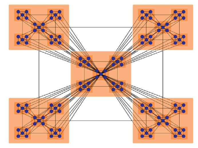
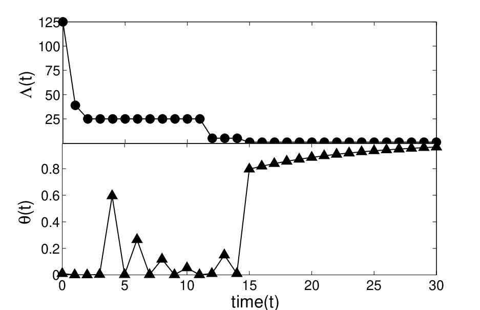
To show that the model can uncover hierarchical structures in different scales, Fig.2 and Fig.3 give two examples of the multi-level community structures. Fig.2 shows the network, which is a hierarchical scale-free network proposed by Ravasz and Barabási in [21]. The regions corresponding to 5 and 25 modules are the most representative in terms of resolution. Next, - proposed by Arenas et al[6] is shown in Fig.3, which is a homogeneous degree network with two predefined hierarchical scales. The first hierarchical level consists of 4 modules of 64 nodes and the second level consists of 16 modules of 16 nodes. The partition of both levels are highlighted on the original networks.
In both examples, the most persistent reveals the actual number of hierarchical levels hidden in a network. The signature of such levels can be quantified by their corresponding length of persistent time. The longer the time persists, the more robust the configuration is. From Fig.2 and Fig.3, we can observe 25 and 16 are the optimal numbers of communities in and - networks owning the longest persistence, respectively. However, 5 modules and 4 modules are also reasonable partitions which show the fuzzy level of the hierarchical networks. These results are in perfect consistence with the generation mechanisms and hierarchical patterns of these two networks.
Furthermore, we also show that the variation tendency of stability in the two cases shed a light on the spin configuration. From Fig.2 and Fig.3, the corresponding stability is not a parabolic shape for the timescales of a specific . Thus we cannot easily find the global optimum. However, there are some local maximal values representing better community structure. Thus, we can find these local maximal timescales corresponding to the desirous number of communities and apply to a specific partition method. Furthermore, the stability will reach the lowest value at the end time of all . The stability begins to increase when it transits to new status. One can use to estimate the modularity property of complex networks, and the larger the the stronger the network community structure. So, one can find the largest corresponding value for a specific number of community and use it to indicate the robustness of modularity structure. For - shown in Fig.3, the stability of 16 communities structure, when , is larger than when . This indicates that the community structure containing 16 modules is more robust than community structure containing 4 modules. Similarly, for network shown in Fig.2, corresponding to 25 communities structure when is larger than when . The robustness of community structure indicated by stability favors small but obvious modules. This is the same as [6][7] and is reasonable for many real networks.


Finally, we emphasize the difference between the stability measure proposed in this paper and the modularity proposed by Newman[1, 3]. is a well-known criterion for evaluating a specific partition scheme of a network. It is defined as “the fraction of edges that fall within communities, minus the expected value of the same quantity if edges fall at random without regard for the community structure” [3, 18, 27, 28]. Different partition schemes will get different values for the same network, and larger ones mean better partitions. While our and try to directly characterize and evaluate the structure property based on network’s spectra, rather than a specific network partition. Therefore, a network only has exactly self-deterministic and values regardless of how many partition schemes it would have, and the larger the the stronger the network community structure. In addition, Fortunato et al[5] pointed out the resolution limit problem of the modularity , that is, there exists an intrinsic scale beyond which small qualified communities cannot be detected by maximizing the modularity. However, as shown in Fig.4, when a clique ring contains cliques with different scales (i.e.,the heterogeneous community size), the intrinsic community structure can be exactly revealed by . With and , we can quantitatively compare the modularity structure of different types of complex networks.


V A new algorithm to detect community
To actually perform the community detection, we propose an approach based on eigenvalue decomposition[29] of correlation matrix . This algorithm allows us to identify multivariate communities across multiple timescales. Based on the above analysis, we correlate the multivariate community structure with the dynamics of the eigenvalues and eigenvectors.
The eigenvalues and eigenvectors of the symmetric and real-valued matrix can be obtained by solving the eigenvalue equation
| (22) |
which has different solutions when time is small. Assume that the eigenvectors are normalized (). Each signature is associated with a specific community (the elements in the vector have the same spin value) and quantifies its strength at a given timescale. For each community , the internal structure is described by the corresponding eigenvector . After normalization (), its components quantify the relative involvement of each node to community by . Combining the signature of the community and the index , the “absolute” involvement of node in a community at time can be described by the following participation index,
| (23) |
Node is considered as belonging to community when the participation index becomes maximal.
From Eq.(23), we observe that participation index evolves as time goes on. When the timescale , all eigenvalues approach to 0 except the largest one, . At this time, all nodes belong to the same community according to the participation index definition. In the other extreme when , the participation matrix actually becomes the eigenvector matrix . All of its columns are different, and the number of communities is equal to the dimension of the matrix. Here we are interested in the optimal partition at an intermediate timescale with large stability , when the spin configuration represents the most robust community structure. So, we first determine the optimal number of communities by using across long time . Then, we pick up the timescale that the stability is maximal between and equals to the optimal number of communities. In many real networks, the formulation of communities is a hard partition and each node belongs to only one cluster after the cluster. This is often too restrictive for the reason that nodes at the boundary among communities share commonalities with more than one community and play a role of transition in many diffusive networks. In our work, the participation index motivates the extension of the partition to a probabilistic setting. It is extended to the fuzzy partition concept where each node maybe long to different communities with nonzero probabilities at the same time and more reasonable for the real world. Finally, we calculate the participation index at the most stable time . The framework of the whole process is summarized in Algorithm 1. In the process of the algorithm, calculate the spin-spin correlation matrix is based on algorithm and costs less than . It is easy to estimate the computational cost of the algorithm is main on the calculation of eigensystem of and for sparse graphs, it is about . Other steps of the process are some simple matrix computations. So finally, we obtain the cost of Algorithm 1 is . Our algorithm is a parameter free method and very easy to implement in real networks.
VI Experiments
In this section, we will benchmark the performance of our algorithm. We designed and implemented three experiments for two main purposes: (1) to evaluate the accuracy of the algorithm; (2) to apply it to real large-scale networks.
VI.1 Benchmark network
We empirically demonstrate the effectiveness of our algorithm through comparison with other five well-known algorithms on the artificial benchmark networks. These algorithms include: Newman’s fast algorithm[1], Danon et al.’s method[32], the Louvain method[33], Infomap[10], and the clique percolation method[27]. We utilize widely used Ad-Hoc network model, which can produce a randomly synthetic network containing 4 predefined communities and each has 32 nodes. The average degree of nodes is 16, and the ratio of intra-community links is denoted as . As decreases, the community structures of Ad-Hoc networks become more and more ambiguous, and correspondingly, their values climb from 0 to 1, as shown in Fig.5.


We use the normalized mutual information (NMI) measure[34] to qualify the partition found by each algorithm. We ask the question whether the intrinsic scale can be correctly uncovered. The experimental results are illustrated in Fig.5, where y-axis represents NMI value, and each point in curves is obtained by averaging the values obtained on 50 synthetic networks. As we can see, all algorithms work well when is more than 0.7 with NMI larger than . Compared with other five algorithms, our algorithm performs the best. Its accuracy is only slightly worse than that of the clique percolation when . However, the complexity of the clique percolation is more than and nearly the same as the time consuming Breadth First Search(). By contrast, the time complexity of our method is very low() and can be easily implemented.
VI.2 US Football network
The United States college football team network has been widely used as a benchmark example[1][28] due to its natural community structure. We used the data gathered by Girvan and Newman[1]. It is a representation of the schedule of Division I American Football games in the 2000 season in USA. The nodes in the network represent the 115 teams, while the edges represent 613 games played in the course of the year. The whole network can be naturally divided into 12 distinct groups. As a result, games are generally more frequent between members of the same group than between members of different groups.


First, we calculate and the corresponding stability and the results are illustrated in Fig.6. Results show that the optimal number of communities is , which perfectly agree with the true situation. The stability reaches when . Then we apply our algorithm to the football team network and partitions the network into 12 communities, which is shown in Fig.7. The correct rate of our method is more than , which means that the detected community structure is in a high agreement with the true community structure. Actually, methods based on optimization of modularity usually can just find 11 communities and the correct rate is low due to the fuzziness of the network. We concludes that the ability of our method to reveal a natural characteristic is valuable for many real networks. Furthermore, our algorithm has identified 5 interesting overlapping nodes which described as yellow triangles. The nodes are all fuzzily lie at the boundary communities and can be viewed as some relative independent clubs which can be interpreted readily by the human eye.
VI.3 Scientific collaboration network
Finally we tested our algorithm on a large-scale network, the scientific collaboration network, collected by Girvan and Newman [22]. The network illustrates the research collaborations among 56,276 physicists in terms of their coauthored papers posted on the Physics E-print Archive at arxiv.org. Totally, this network contains 315,810 weighted edges. For visualization purpose, our algorithm outputs a transformed adjacency matrix (in which the nodes within the same community are grouped together) with a hierarchical community structure. From the transformed matrix of Figs.8, one can observe a quite strong community structure, or a group-oriented collaboration pattern. Among these physicists, three biggest research communities are self organized regarding to three main research fields: condensed matter, high-energy physics (including theory, phenomenology and nuclear), and astrophysics.
The cumulative distribution of community sizes in power plot is shown in Fig.8 and it is a typical scale-free distribution which exists broadly in real world. In total, 737 communities were detected by the optimal community stability, the maximum size of those communities is 195, the minimum size is 2, and the average size is 76. Among these communities, 1,433 of 6,931 pairs of communities have fuzzy participation index with each other. largest communities contain of the nodes, while the others are relatively small. The three largest communities correspond closely to research subareas. The largest is solid-state physics, the second largest is super-nuclear physics, and the third is theoretical astrophysics. Furthermore, a subnetwork including eight communities in is shown in Fig.8 and four regions including 10 overlapping nodes are highlighted by four circles, which were detected according to the participation index . The partition result is completely the same as the results in Refs.[22] and [28]. The efficient performance in large real network indicates that our method is useful for further researches in various fields.


VII Conclusion
In summary, we have presented a more theoretically-based community detection framework which is able to uncover the connection between network’s community structures and spectrum properties of Potts model’s local uniform state. We demonstrate that important information related to community structures can be mined from a network’s spectral signatures through a Markov process computation, such as the stability of modularity structures and the optimal number of communities. Based on theoretical analysis, we further developed an algorithm to detect fuzzy community structure. Its effectiveness and efficiency have been demonstrated and verified through both the simulated networks and the real large-scale networks.
Acknowledgments: We are grateful to the anonymous reviewers for their valuable suggestions which are very helpful for improving the manuscript. The authors are separately supported by NSFC grants 11131009, 60970091, 61171007, 91029301, 61072149, 31100949, 61134013 and grants kjcx-yw-s7 and KSCX2-EW-R-01 from CAS.
References
- [1] M.E.J.Newman, Phys. Rev. E. 69, 066133(2004).
- [2] M.E.J.Newman, M.Girvan, Phys. Rev. E. 69, 026113(2004).
- [3] M.E.J.Newman, Proc. Natl. Acad. Sci 103, 8577-8582(2006).
- [4] A.L.Barabási, R.Albert, Science 286, 509-512(1999).
- [5] S.Fortunato, M.Barthelemy, Proc. Natl. Acad. Sci 104, 36(2007).
- [6] A.Arenas, A.Fernandez, S.Gomez, New. J. Phys 10, 053039(2008).
- [7] A.Arenas, A.Diaz-Guilera, C.J.Perez-Vicente, Phys. Rev. Lett 96, 114102(2006).
- [8] J.C.Delvenne, S.N.Yaliraki, M.Barahona, Proc. Natl. Acad. Sci 107(29), 12755-12760(2010).
- [9] W.N.E, T.Li, E.Vanden-Eijnden, Proc. Natl. Acad. Sci 105, 7907-7912(2008).
- [10] M.Rosvall, C.T.Bergstrom, Proc. Natl. Acad. Sci 105(4), 1118-1123(2008).
- [11] H.Zhou, Phys. Rev. E 67, 041908(2003).
- [12] F.Y.Wu, Rev. Mod. Phys 54(1), 235-268(1982).
- [13] M.Blatt, S.Wiseman, E.Domany, Phys. Rev. Lett 76, 3251-3255(1996).
- [14] S.Wiseman, M.Blatt, E.Domany, Phys. Rev. E 57), 3767-3783(1998).
- [15] H.Agrawal, E.Domany, Phys. Rev. Lett 90, 158102(2003).
- [16] J.Reichardt, S.Bornholdt, Phys. Rev. Lett 93, 218701(2004).
- [17] H.J.Li, Y.Wang, L.Y.Wu, Z.P.Liu, L.Chen, X.S.Zhang, Eur. Phys. Lett 97, 48005(2012).
- [18] X.S.Zhang, R.S.Wang, Y.Wang, J.Wang, Y.Qiu, L.Wang, L.Chen, Eur. Phys. Lett 87, 38002(2009).
- [19] T.Ott, A.Kern, W.Steeb, R.Stoop, J. Stat. Mech 11, 11014(2005).
- [20] S.Wang, R.H.Swendsen, Physica(Amsterdam) 167A, 565(1990).
- [21] E.Ravasz, A.L.Barabási, Phys. Rev. E 67, 026112(2003).
- [22] M.Girvan, M.E.J.Newman, Proc. Natl. Acad. Sci 99, 7821-7826(2002).
- [23] J.Shi, J.Malik, IEEE Tans.On Pattern Analysis and Machine Intelligent 22(8), 888-904(2000).
- [24] M.Fiedler, Algebraic Connectivity of Graphs. Czechoslovakian Math J 23, 298-305(1973).
- [25] R.Guimera, L.A.N.Amaral, Nature 2, 895-900(2005).
- [26] B.D.Hughes, Random walks and random environments: Random walks, Clarendon Press, Oxford, UK 1, (1995).
- [27] G.Palla, I.Derényi, I.Farkas, T.Vicsek, Nature 435, 814-818(2005).
- [28] Z.P.Li, S.H.Zhang, R.S.Wang, X.S.Zhang, L.Chen, Phys. Rev. E 77, 036109(2008).
- [29] C.Allefeld, M.Muller, J.Kurths, J, Int. J. Bifurcat. Chaos 17, 3493(2007).
- [30] J.Shi, J.Malik, IEEE Trans.Pattern Anal. Mach. Intell 22, 8888(2000).
- [31] A.Azran and Z.Ghaharmani, IEEE Computer Society Conference on Computer Vision and Pattern Recognition Vol. I, 190-197(2006).
- [32] L.Danon, J,Duch, D.Guilera, A.Arenas, J. Stat. Mech 29, P09008(2005).
- [33] V.D.Blondel, J.L.Guillaume, R.Lambiotte, E.Lefebvre, J. Stat. Mech 10, P10008(2005).
- [34] A.Lancichinetti, S.Fortunato, Phys. Rev. E 80, 056117(2009).