Power-law statistics and universal scaling in the absence of criticality
Abstract
Critical states are sometimes identified experimentally through power-law statistics or universal scaling functions. We show here that such features naturally emerge from networks in self-sustained irregular regimes away from criticality. In these regimes, statistical physics theory of large interacting systems predict a regime where the nodes have independent and identically distributed dynamics. We thus investigated the statistics of a system in which units are replaced by independent stochastic surrogates, and found the same power-law statistics, indicating that these are not sufficient to establish criticality. We rather suggest that these are universal features of large-scale networks when considered macroscopically. These results put caution on the interpretation of scaling laws found in nature.
Keywords:
Avalanches, Power laws, self-organized criticality, neuronal datapacs
02.50.-r, 05.40.-a, 87.18.Tt, 87.19.ll, 87.19.lc, 87.19.lmI Introduction
Power law statistics are ubiquitous in physics and life sciences. They are observed in a wide range of complex phenomena arising in natural systems, from sandpile avalanches to forest fires [1, 2], earthquakes amplitude solar flares, website frequentation as well as economics [3]. These distributions reveal unusual properties: the observed quantity has no typical scale, and is not well characterized by its mean (when it exists): it is distributed over orders of magnitudes and large deviations are not exceptionally rare, in the sense that extreme events are far more likely than they would be, for instance, in a Gaussian distribution. These singular properties, combined with their ubiquity in nature, has attracted wide attention in applied science.
A number of theories were proposed in order to account for the presence of such power-law distributions. Some theories use an analogy with statistical physics systems and associate the presence of power-law scalings as the hallmark that the system could be operating at a phase transition. These theories associate power-law to a so-called notion of criticality: classically, in statistical physics, critical phenomena are the behaviors occurring in systems in association with second order phase transitions. These are largely thought to be universal although no proof was provided yet. Indeed, a number of statistics are found in vastly distinct models, and particularly in the Ising model [4] poised at its phase transition. The critical regime thus occurs only at very specific parameters values. At this regime the properties of the system are particularly singular; in particular, a number of statistics are scale-invariant including for instance the size, duration and shape of collective phenomena. The seminal work of Bak, Tang and Wiesenfeld on the Abelian sandpile model [5] largely popularized the hypothesis that criticality may be the origin of power-laws observed in nature. Indeed, despite the fact that parameters for criticality are very rare, systems may self-organize naturally at criticality (at the phase transition point) without requiring fine tuning by a mechanism called self-organized criticality (SOC) [1]. This remarkable theory has sometimes led to the conclusion that natural systems were critical based on the identification of power-law relationships in empirical data (see [5, 2] for reviews).
While power laws, as well as phase transition (thus criticality) are well identified in models, a number of authors have underlined the importance of being cautious when claiming power-law behavior in finite systems, questioning their relevance or usefulness [6, 7]. In particular, Stumpf and Porter in [6] aptly noted the importance to take a nuanced approach between theoretical and empirical statistical support reporting a power-law, as theories arise from infinite systems while and real systems and usual datasets are finite.
In physics, several alternative theories were proposed to account for the presence of power-laws (see e.g. [3] for a review). In particular, it was noticed very early that a pure random typewriter (a monkey sitting at a typewriter) would generate texts with a power-law distribution of word frequencies [8] identical as the one observed in data. This work brilliantly showed that power-law may arise from purely stochastic mechanisms, evidencing that some power-laws distributions may not reflect deep structures in the data. Li [9] formalized Miller’s theory, highlighting the fact that combinations of exponentials naturally yield power-law relationships. Bouchaud and others [10, 11] noted that inverse of regularly distributed quantities may show power-law distributions. Newman and colleagues showed that random walks generate several statistics scaling as power-laws [3], Yule introduced a process with broad applications, particularly in evolution, naturally associated to power-law distributions, and Takayasu and collaborators [12, 13, 14] showed that systems with aggregation and injection naturally generate clusters of size scaling as a power-law with exponent . In neuroscience, Benayoun, Wallace and Cowan have shown that neuronal networks models in a regime of balance of excitation and inhibition also provide power-law scalings of avalanches [15]. All these mechanisms are independent of any phase transition and arise away from criticality from a particular way of considering a random process.
The hypothesis that networks of the brain operate at criticality was introduced a decade ago with the development of recording techniques of local populations of cells and the analysis of specific events corresponding to collective bursts of activity separated by periods of silence. The first empirical evidence that neuronal avalanches may show power-law distributions of duration or size was derived from the analysis of neuronal cultures in vitro activity [16]. Based on an analogy with the sandpile model, these bursts were seen as “neuronal avalanches”, and were apparently distributed as a power-law with a slope close to , consistent with the distribution of sandpile avalanches. These in vitro findings were based on indirect evidences of spiking derived from local field potentials, extracellular signals associated with the summation of postsynaptic potentials (bursts produce negative peaks in the LFP signals) and affected by a number of events unrelated with spiking activity. Similar LFP statistics were later found in vivo in the awake monkey [17] and in the anesthetized rat [18]. These empirical evidences were used to draw strong conclusions on neural coding: the presence such power-laws would ensure maximized information capacity, dynamic range and information transmission [19, 20]. However, the method of analyzing the amplitude of negative LFP peaks was shown to produce spurious power laws scalings [21] regardless of the spike activity of cells. Indeed, identical scalings were found in surrogate data, positive LFP peaks (that are independent of spiking activity), and also arise in elementary purely stochastic signals, such as excursions of Ornstein-Uhlenbeck processes through thresholds away from the mean, or in one-dimensional random walks [22, 23]: both duration and time of excursions show power-law statistics, and display shape invariance. It was further shown in that both in data and surrogate models, statistical significance of these power-laws of LFP peak was poor, and depended on the threshold chosen. In [24], Dehghani and collaborators have made a statistical analysis combining multielectrode in vivo recordings from the cerebral cortex of cat, monkey and human, and did not confirm the presence of power-laws. The data rather showed an optimal fit with two independent exponential processes.
The poor statistical significance of LFP avalanche analysis and the ambiguous results it yields has motivated an in-depth exploration of in vitro spiking data of cultures of neurons [25]. In this remarkable work, the authors used multi-unit data from in vitro cultures and addressed a number of properties of critical systems reported by Sethna et al unified theory of criticality of statistical systems [26]. Of crucial importance in this theory are power-law scalings of specific events and the relationship between the different scaling exponents. Friedman and collaborators [25] revealed that the data was consistent with Sethna et al theory, since power-law scalings of both avalanche size and duration were reported, with slopes consistent with the critical exponents of and respectively, but also the existence of a universal mean temporal profiles of firing events collapsing under specific scaling onto a single universal scaling function, thereby providing more substantial analogy between this in vitro system with statistical physics models at criticality.
In the present paper, we show that these observations can arise naturally in neuronal systems that are not at criticality. We also provide a theoretical explanation for this, as well as analytic access to some of the relevant properties of such systems.
II Avalanches in spiking network models
We start by investigating the avalanche distributions generated by the classicalmodel of spiking neuronal network with excitatory and inhibitory connections introduced by Nicolas Brunel in [27]. This model describes the interaction of neurons described through their voltage that decays to reversal potential in the absence of input, receives external input and spikes from interconnected cells, and fire action potentials when the voltage exceeds a threshold . In detail, the voltage of neuron satisfies the equation:
| (1) |
while , and where denotes the time constant of the membrane and its resistivity. The input received by the neuron are Dirac s. Neuron receives the th impulse of neuron , emitted at time , after a delay denoted and assumed constant, which alters its membrane potential of a quantity proportional to . Brunel’s model assumes that these coefficients are zero except for a fixed number of cells randomly chosen in the excitatory and inhibitory populations, for which the coefficient have fixed values and respectively (see [27] for details). This model is particularly interesting very for its versatility and ability and to produce diverse spiking patterns. One can classify the regimes of activity in terms of levels of synchrony and regularity, and different regimes emerge as a function of the relative levels of excitation and inhibition and the input, that can be identified through the computation of precise bifurcation curves [27]. The thus obtained regimes are termed activity states, to distinguish these from the statistical mechanics notion of phase: the regimes are here separated by bifurcations occurring in the mean-field limit of the system. Of special interest are the Asynchronous Irregular (AI) states, in which neurons fire in a Poisson-like manner, with no period of silence (hence no avalanche). This activity is evocative of the spike trains observed experimentally in awake animals. Such sparsely-connected networks can also display periods of collective activity of broadly distributed duration interspersed by periods of silence, called Synchronous Irregular (SI) regimes, known to reproduce the qualitative features of spiking in anesthetized animals or neuronal cultures. Although partially ordered and partially disordered, SI regimes occur for a wide range of parameter values (all in inhibition-dominated regimes) [27] and are not very sensitive to modifications of biophysical parameters. The SI regime is not at a transition in the activity regime; within this region, chaotic activity takes place. Indeed, inhibition dominates the excitation, thus when the activity spreads throughout the network, it triggers massive inhibition that naturally silences the network. This is what we observe in simulations of the Brunel model (Fig. 1)11 1 We used the algorithm freely available on ModelDB.. We investigate the statistics of spike units in both cases (see Fig. 1).

First, in the AI state, the sustained and irregular firing does not leave room for repeated periods of quiescence at this network scale, preventing the definition of avalanches (see raster plot in Fig. 1(B)) 22 2 Sub-sampling of the network may lead to find periods of quiescence, whose statistics will depend on the network size. However, these are not robust statistical quantities to define a critical regime.. This sharply contrasts with the SI state, in which we can define avalanches which display the same statistics assumed to reveal criticality in cultures [25]. Fig 1(A) represents the raster plot with typical avalanches taking place. Strikingly, both avalanche duration and avalanche size show excellent fit to a power law, validated by Kolmogorov Smirnov test of maximum likelihood estimator [30], and the exponents found are consistent with those found in neuronal cultures [25]. In particular, we find that the size of the avalanches (number of firings during one avalanche) apparently scales as with (Fig. 1(C)), close to the theoretical value of (plotted on the figure for indication), and to the neuronal culture scaling ( reported in [25]). Using the Kolmogorov-Smirnov test [30], we have tested the hypothesis that the data are distributed as a power-law, and validated the hypothesis (Kolmogov-Smirnov distance , p-value . This is also the case of the distribution of the duration of the avalanches, found scaling as with (Fig. 1(D)), close to the theoretical value of for critical systems and from the experimental value of found in neuronal cultures [25]). The Kolmogorov-Smirnov distance with a pure power law is very low, evaluated at , which leads to a high p-value , validating clearly the hypothesis of a power-law distribution of avalanche durations. Similar to what was observed experimentally, the fit is valid on two octaves, and drops down beyond33 3 The Kolmogorov-Smirnov statistical tests is not affected by events of very small frequency.. This exponential drop is classically related to subsampling effects. We validated the presence of finite-size cutoffs by varying the size of the system, and found indeed that as the network size increases, the fit with a power-law distribution is valid on larger time intervals and the cutoff only arises at later times (see Supplementary Figure 6). Also consistent with neuronal data and crackling noise, we found that the average avalanche size scales very clearly as a power of its duration, but with a positive exponent , not consistent with the crackling noise relationship between exponents
| (2) |
that predicts an exponent equal to , but however quantitatively consistent with the in vitro data of [25]. We have also investigated the shape of the avalanches of different durations. We have found that, similarly to critical systems or to in vitro data, the avalanche shapes collapsed onto a universal scaling function (Fig. 1E) when time is rescaled to a unit interval and shape rescaled by where is the power law exponent of the average size.
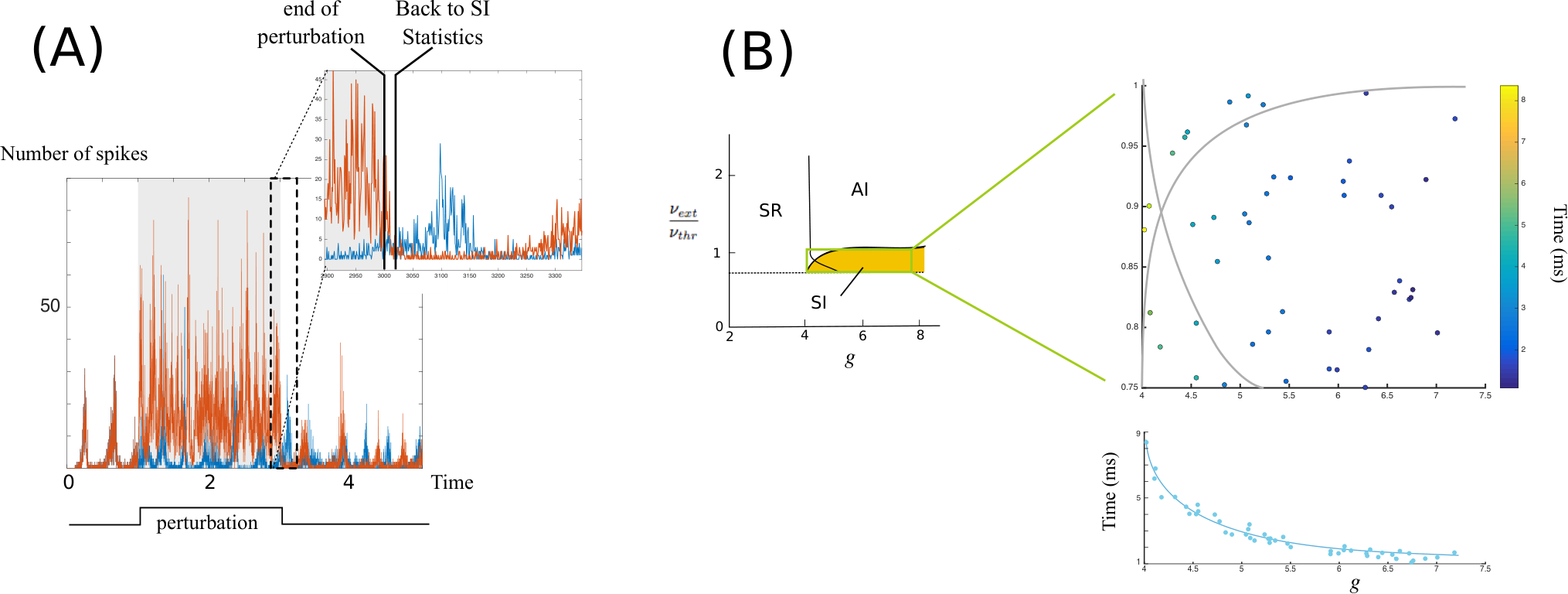
These scalings are not specific to the particular choice of parameters used in our simulations: we consistently find, in the whole range of parameter values corresponding to the SI state of Brunel’s model, and in particular, away from any transitions, similar apparent power-law scalings with similar scaling exponents (see supplementary Figure 7). Moreover, we confirmed, in addition to the fact that this regime is away from all transitions between the different network activity, that the system is not at criticality, by showing that relaxation towards the SI regime after perturbation is fast (within milliseconds) within the region considered, although it does slow down close to the transition point (see supplementary Figure 8). We conclude that these statistics are valid in a whole regime of the system where the activity is synchronous irregular, and neither at a transition of the model nor in a regime consistent with the slow decay of perturbations associated to critical regimes. Therefore, finding power-law statistics in neuronal avalanches with exponents and do not reveal that the system operates at criticality, but rather seems a property of synchronous irregular states.
The SI states are prominent in neuronal activity, especially in anesthesia and neuronal cultures. It is precisely in these situations that power-law distributions of spike avalanches were reported experimentally [16, 18]. This regime differs from the awake activity where neurons fire in an AI manner. In these regimes, power-laws and criticality were reported based on LFP recordings [17]. We will come back to experimental evidences of power-laws in local-field potentials recordings of the activity in section V.
III Avalanches and Boltzmann molecular chaos property
The observation of such scaling relationship in simple models of neuronal networks away from criticality and for a broad range of parameter values suggests that the observed scaling is related to properties of the systems that are independent of the notion of criticality and that may be relatively general. These may therefore be related to the properties of the network activity, that we now describe in more detail.
III.1 Propagation of chaos in neural networks models
The classical theory of the thermodynamics of interacting particle systems states that in large networks (such as those of the brain), the correlations between neurons vanishes. This is also known as Boltzmann molecular chaos hypothesis (Stoßzahlansatz) in reference to the hypothesis that the speed of distinct particles should be independent, key to the kinetic theory of gases of Ludwig Boltzmann [32]. In mathematics, this property is called propagation of chaos, and is rigorously defined as follows:
Definition 1.
For a sequence of measures on . The sequence is said -chaotic if for any and a set of indexes independent of , we have converge to independent copies of as .
In our context, in the limit of large networks, neurons behave as independent jump processes with a common rate, which is solution of an implicit equation. This property is at the core of theoretical approaches to understand the dynamics of large-scale networks [27, 33, 34, 35]. In the case of Brunel’s model, it is shown that since two neurons share a vanishing proportion of common input in the thermodynamic limit, allowing to conclude that the correlation of the fluctuating parts of the synaptic input of different neurons are negligible. This leads the authors to conclude that the spike trains of different neurons are independent point processes with an identical instantaneous firing rate that is solution of a self-consistent equation (see [27, p. 186, first column]). In that view, except in the case of constant firing rate (the asynchronous irregular state), neurons always show a certain degree of synchrony due to the correlations of the instantaneous firing rates of different neurons.
Mathematically, several methods were developed for interacting particle systems and gases (see e.g. [36] for an excellent review). It is shown that generically, systems of interacting agents, with sufficient regularity, show propagation of chaos. All these results are in particular valid for neuronal networks, as was shown recently in a number of distinct situations. Large limits and propagation of chaos was demonstrated for large networks of integrate-and-fire neurons [37], firing-rate models with multiple populations [38], for conductance-based models even in the large time regime [39], and was shown to hold in realistic network models incorporating delays and the spatial extension of the system [40, 41]. Rigorous methods of convergence of particle systems show that the empirical measure of the system:
converges in law towards a unique solution. A very powerful and universal mathematical result demonstrated in [42, Lemma 3.1] ensures that that the convergence of the empirical measure of a particle systems towards a unique measure implies propagation of chaos. Several methods may be used to show convergence of the empirical measure, including in the case of neuroscience, coupling methods [41], compacity estimates [37] or large deviations [43].
These results indicate that a universal form of activity emerges from neural networks, whereby neurons are independent copies of the same process. Before investigating the avalanche statistics of such regimes of activity, let us discuss the plausibility of the existence of these regimes in neuronal data.
III.2 Decorrelation in experimental data and models
In natural environments, regularity of sensory input to the brain may create strong and long-range correlations in space and time [44, 45, 46, 47]. It soon appeared that these correlations would be detrimental for the brain to encode sensory stimuli and detect changes efficiently [48, 49]. Theoretical models of the visual system in particular have shown that decrease of redundancy by decorrelation was important for efficient encoding of natural images [50, 51, 52]. This was confirmed experimentally. In [53], the authors used high density two-dimensional electrode array and found in particular a marked exponential decay of correlation of excitatory cells. An clear confirmation of decorrelation even for closeby cells receiving similar input was recently brought in a remarkable experimental work where chronically implanted multielectrode arrays were developed and implanted in the visual cortex of the macaque [54]. This protocol produced exquisite data allowing to show that even nearby neurons, generally thought to be strongly connected and to receive a substantial part of common input showed a very low level of correlation. Similar decorrelation results were reported in the rodent neocortex [55] with the same level of accuracy.
The origin of this decorrelation is still controversial and several assumptions were formulated, including the role played by adaptation ionic currents that could play central role in temporal decorrelation [56], negative correlations associated with the co-evolution of excitatory and inhibitory cells activity [55], or sophisticated and robust mechanisms relying on neuronal nonlinearities and amplified by recurrent connectivities [57], that was compatible with pattern decorrelation observed in the olfactory bulb of the zebra fish.
All these experimental findings confirm that regimes in which neurons are independent are plausible representations of neural networks activity. We now investigate the avalanche statistics of such networks.
III.3 Statistics of networks in the molecular chaos regime
Both the mathematical analysis of neuronal network models and fine analysis of the structure of spike trains motivates the study of ensembles of neurons that are independent but with common non-stationary statistics. The simplest model made of one could think of is to consider a collection of independent Poisson processes with identical time-dependent rates.
In that view, cells with constant firing rates resemble AI regimes. To generate a stochastic surrogate of the SI regime, the common rate of the cells should display non-periodically periods of silence. An obvious choice would be to replay the rates extracted from the SI state, and indeed such a surrogate generated power-law statistics (not shown), but in this case we could not rule out whether the power-law statistics are encoded in the rate functions. To show that this is not the case, we generated a surrogate independent of the rate functions, by using a common rate of firing of the neurons given by the positive part of the Ornstein-Uhlenbeck process:
with a Gaussian white noise. This choice is interesting in that although periods of silence do not occur periodically, the duration between two such silences have a finite mean. Actually, the distribution of excursions shape and duration of the Ornstein-Uhlenbeck process are known in closed form [58]. These distributions are, of course, not heavy tailed: they have exponential tails with exponent which is the timescale of decay of the process.
We investigated the collective statistics of independent realizations of Poisson processes with this rate. The resulting raster plot is displayed in Fig. 2(A). While the firing is an inhomogeneous Poisson process, macroscopic statistics show power-law distributions for the size (, Fig. 2(B)) and for the duration (, Fig. 2(C)), both statistically significant [30] and consistent with critical exponents. Again, a linear linear relationship between average avalanche size and duration is found, with a coefficient evaluated to and explaining all the variance but . Again, this coefficient is not consistent with the crackling relationship (2). Notwithstanding, we found that the averaged shape of avalanches of a given duration collapse on one universal curve when the amplitude is rescaled by the duration to the power (Fig. 2(D,E)).

Of course, these statistics are not related to the nature of the rate chosen. We display in Supplementary Fig. 9 for instance the avalanche statistics of independent Poisson processes with rate given by the positive part of a reflected Brownian, and we find exactly the same power-law statistics of avalanche shapes and durations, as well as a very nice collapse of avalanche shapes.
III.4 Analytical derivations in the stationary and slow rate regime
In this simple model, it is actually very simple to indeed compute explicitly the distribution of avalanche duration for instance. Disregarding the Poisson nature of the firings and the type of rate chosen, we can indeed write down the probability for an avalanche of duration to occur at a specific time. These distributions can be computed analytically in cases where the spiking is described by a point process. In that case, denoting by the probability for a neuron to spike in the time interval , the probability to observe an avalanche of size starting at time in a collection of independent realizations is
Assuming stationarity, the probability of finding an avalanche of duration is given by
where denotes the joint probability for the firing rate to have a specific sequence of values .
This formula remains quite complex. Assuming now that the rate is extremely slow compared to the avalanches, one can simplify further the probability of of an avalanche of size :
thus with a simple change of variable:
As expected, when , the probability of having an avalanche of prescribed, finite duration goes to zero as . The typical shape of the distribution can be obtained by rescaling this probability by . Since we are interested in the logarithmic shape of the distribution, we disregard any multiplicative constant. As , we thus obtain that the probability profile converges towards a universal limit independent of the particular shape of the distribution , precisely given by:
which is indeed a power law with exponent , identical to the one arising in critical systems, consistent with those reported in neuronal data [25], in neuron models (Fig. 1) and in surrogate systems (Fig. 2).
We now show that this extends to the distribution of avalanche size and the scaling of the mean avalanche size with duration. Indeed, the size of avalanches of duration have a binomial distribution, corresponding to successes among independent Bernoulli variables with probability of success . Moreover, De Moivre-Laplace theorem [59] ensures convergence as increases towards a normal variable with mean and variance with . Using again our separation of timescale and stationarity hypotheses, we find the probability the probability of finding an avalanche of size and duration averaged on the firing rate:
which converges, as , towards:
We thus obtain at leading order the size distribution:
| (3) |
It is hard to further simplify this formula, but it can be easily evaluated numerically. We depict the result of this computation in Fig. 3, and illustrate the apparent power-law scaling with slope .
Eventually, we obtain for the average size of avalanches of duration :
We thus conclude that while a power-law relationship persists between and , the scaling exponent is not related to the exponents of the power-law of size () and duration () distribution through Sethna’s crackling noise relationship, which would predict an exponent equal to . Importantly, we note that the exponent found here is quantitatively perfectly consistent with the exponent found in in vitro data [25] in the neural network model (Fig. 1) or surrogate Poisson system (Fig. 2).
IV Spike pattern entropy and information capacity
We have thus proved that power-law distributions of avalanches do not necessarily reveal that the network is operating at criticality. However, a number of theories have proposed that operating at criticality was an optimal regime of information processing in the brain, maybe selected by evolution as a useful trait for the nervous system [60, 61, 62, 60, 19, 63, 64]. The question that arises is thus whether these theories break down when power-law statistics no more arise from the system operating at criticality, but from a mean-field Boltzmann chaos regime.
In order to address this outstanding question, we came back to the methods used in order to demonstrate optimality of data processing capabilities at criticality. These theories rely on the computation of the information capacity of the network in different activity regimes evaluated, following Shannon’s information theory, as the entropy of the patterns of spike fired. In detail, a spike pattern in a network of size is a -uplet , with (resp. ) if neuron has fired (resp., not fired) in a specific timebin. If denotes the probability of occurrence of spike patterns, the entropy is given by:
In order to test whether our theory accounting for the emergence of power-law distributions in the absence of criticality challenges high information capacity of neuronal networks, we computed the information capacity of Brunel’s model in different regimes (see Fig. 4). The numerical results show that this is not the case, and the information capacity is maximal in the SI regime where power-law statistics of avalanches were observed. However, we observe no difference between entropy levels in the SI or AI states. Therefore, we conclude that the maximality of entropy is not necessarily related to the emergence of power-law statistics.
These observations can be well understood heuristically. Indeed, the entropy of spike patterns is a measure of the variability of possible spike patterns observed in the course of neuronal activity. The diagram of Fig. 4 is thus not surprising. Indeed, while the diversity of spike patterns is reduced in the highly synchronized regular regimes, it will be large in the irregular regimes, both synchronized asynchronous 44 4 In the models based on branching processes with parameter , it is clear that the maximal diversity arises at criticality, where the entropy is larger than in the sub-critical regime (only patterns with a small number of spikes) or in the super-critical regime (patterns with a large number of spikes).. In other words, entropy is maximized within irregular regimes where more diverse patterns are fired, and this independently of the underlying mechanisms supporting the emergence of the irregular activity.

V Local field potentials are ambiguous measures of criticality
We have thus shown that discarding the criticality assumption does not degrade the quantifications of network efficiency This being said, we are facing an apparent contradiction. Indeed, our theory provides an account for the presence of critical statistics in networks in the SI regime, but discards AI states as possibly having critically distributed avalanches. Evidences of critical statistics of avalanches in-vivo in the awake brain have been reported, but are more scarce and controversial. Unlike neuronal cultures, the activity in the awake brain does not display bursts separated by silences, but is sustained. Using a macroscopic measurement of neuronal activity, the Local Field Potential (LFP), power laws could be shown from the distribution of peaked events [17]. The motivation to use negative LFP peaks to deduce information from the distribution of spike avalanches relied on the fact that the amplitude of these peaks correlated with firing activity [19, 16].
However, this monotonic relationship between the number of spikes and the number of spikes do not imply that there should exist a relationship between the distribution of peak amplitude and avalanches. Moreover, it was shown that power-laws naturally emerge from the random nature of the signal and the thresholding procedure used in this analysis, and moreover these power-laws may not be statistically significant [21]. Indeed, no power-law scaling could be found from unit activity, which were better fit by double-exponential distributions [24]. These analyses rather suggest that the power-law statistics of LFP peaks does not reflect scale-invariant neural activity.
In an attempt to clarify this, we investigate here whether the distribution of LFP peaks can display power-law scaling in spiking networks or in their stochastic surrogates. To obtain a more biophysical model where LFP can be defined, we considered the current-based Vogels and Abbott model [66] which provides a biologically realistic model of spiking network displaying asynchronous irregular and synchronous regular states, and in which synaptic currents are described by exponentially decaying functions with excitation and inhibition having distinct time constants (in place of Dirac impulses in the Brunel model (1) see [66] for details). Simulations of the model provide an instantaneous distribution of postsynaptic currents, from which we computed LFP signals.
In detail, we have considered a spatially extended neural network of units randomly located on a 2-dimensional square and satisfying the by the Vogels-Abbott model. We evaluated an LFP signal from the postsynaptic currents according to Coulomb’s law [67]:
where is the electric potential at the electrode position, = 230 cm is the extracellular resistivity of brain tissue, are the synaptic currents of and is the distance between and electrode position. Remarkably, applying to this more sophisticate model the same procedures as in the original paper [17], we found that the method cannot distinguish between structured or non-structured activity: for a fixed firing rate and bin size, we have been comparing in Figure 5 the LFP statistics of the avalanche duration in a network of neurons in the AI regime (A) or in the SI regime (C) that shows partial order of the firing and saw no difference. We also compared the statistics to those of independent Poisson processes with constant rate (B): the three instances show power-law scaling of avalanche duration, with the same exponent, that seem to rather be related to the firing rate and bin size than to the form of the network activity. The scaling coefficient is again, close from , and varies with bin size. Clearly, in this case, the dynamics of LFP peaks cannot distinguish between critical and non-critical regimes.

VI Discussion
In this paper, we have evaluated how power-law statistics and universal scaling can arise in the absence of criticality. We first outline the novel contributions of the present manuscript, then we discuss their significance.
The contributions of the present manuscript are the following:
- (i).
We first investigated the avalanche statistics of spiking neural networks models (Section II). We showed that these networks display power-law statistics with the critical exponents -3/2 and -2, as well as collapse of the shapes of avalanches. This observation is robust and valid for a wide region of parameters corresponding to synchronous irregular activity in such networks, and thus away from any transition point (i.e., away from criticality).
- (ii).
This robust numerical observation led us to investigate theoretically how such statistics can emerge from the collective activity of spiking networks. One ubiquitous property of large neural networks models is that neurons behave as independent processes with the same statistics. This property, termed Boltzmann’s molecular chaos regime in statistical physics, or propagation of chaos in mathematics, is universal in the dynamics of large-scale networks. We reviewed such properties in models, as well as recent experimental evidence supporting this decorrelation between the dynamics of cells.
- (iii).
We next tested the hypothesis that power-laws may emerge from such large systems of weakly correlated units with similar statistics. We introduced and investigated numerically the dynamics of a surrogate network made of independent neurons sharing the same statistics (Section III.3). Surprisingly, despite the simplicity of these systems, they display precisely the same power-law statistics of avalanche duration and size with the same exponents and shape collapse as fully-connected networks.
- (iv).
This surrogate model is simple enough to derive in closed-form the statistics of the duration and size of the avalanches. Using this analytic expression, we demonstrate that the ‘critical’ exponents emerge naturally in large-scale systems (operating within the Boltzmann chaos regime), without the need to invoke criticality (Section III.4).
- (v).
Current literature indicate that criticality is an optimal information processing regime for the brain. We considered the same measures of information capability (entropy of spike trains) on our biologically plausible models and showed that indeed, information is maximized in the SI regime where power-laws emerge. However, we show that this is not exclusive of the SI regime but same levels of entropy are found in AI regimes where no avalanche can be defined.
- (vi).
Finally, we also addressed the presence of power-law scalings observed in LFP recordings by simulating such signals emerging from more realistic neuronal network models with excitatory and inhibitory cells. Surprisingly, we observed that power-laws with the same exponents as observed in experiments are found in all regimes tested. This exponents persisted when neurons were replaced by independent Poisson processes. This clearly indicates that power-law scalings in LFPs do not constitute any proof of criticality in the underlying system.
All together, these numerical and theoretical findings provide a new interpretation for the emergence of power-law statistics in large-scale systems, independent of the notion of criticality. We propose to explain the emergence of such scaling based on Boltzmann molecular chaos regime, known to govern the dynamics of most large-scale interacting systems [36, 27, 40]. In other words, power-law and universal scaling functions can be due to a mean-field effect in systems made of a large number of interacting units. Of course, this theory does not hypothesize that the elements considered (here, neurons) are disconnected in reality. To the contrary, the fact that the critical exponents still resist the removal of interconnections shows that such exponents do not need criticality to be explained.
The main mechanism explored here, Boltzmann’s molecular chaos, is a universal feature of many statistical systems. The very particular structure of different particles activity it induces, namely statistical independence of the particles behavior together with a correlation in the law, may induce as we have observed, the same type of power-laws as in critical systems, with universal coefficients that are consistent with those found in critical systems. In agreement with this theory, we have seen that the same statistics are reproduced by a sparsely connected network and a surrogate stochastic process where the periods of firing and silences are themselves generated by another stochastic process. This interpretation suggests that similar scaling relationships shall arise in more realistic neural network models with fixed connectivity patterns, in particular including axonal propagation delays (constant delays are already present in Brunel model), dendritic structure, spike frequency adaptation, non-instantaneous synaptic transmission. Indeed, most of these elements will make the intrinsic dynamics of each cell more complex, but we do not expect that this complexity could affect the fact that these systems operate within the Boltzmann molecular chaos regime. Notwithstanding, models including synaptic plasticity, which is the process by which the brain acquires skills and stores memories, may not belong to the class of systems described in this paper. Indeed, in such systems, the connectivity patterns vary depending on the pairwise correlations of cells activity, and this relationship may compete with the establishment of Boltzmann’s molecular chaos regime. While this may not occur in the adult brain where plasticity is much slower than neuronal activity, distinct phenomena not described by our model may occur occur during the critical periods of brain development, when plasticity occurs at a faster timescale. Further experimental and theoretical investigations are necessary to characterize avalanche distributions in these systems, as well as to compute correlation levels to test if the decorrelation characteristic of Boltzmann’s molecular chaos occurs.
Interestingly, a network operating in Boltzmann’s molecular chaos regime can be interpreted as a high dimensional system with hidden variables, as studied recently in [68, 69]. In these contributions, the authors investigate the rank distribution of high dimensional data with hidden latent variable, and show that such systems display Zipf law scaling (power-laws with slope in the rank distribution) that generically arise from entropy consideration, and using the elegant identity between entropy and energy shown in [70]. While these developments do not generalize here, Boltzmann molecular chaos provides a natural explanation for the emergence of weakly correlated units with similar probability laws: in the neural network system case, the common rate could be seen as a latent variable, and both independence and irregularity build up only from the interactions between cells. As a result of this theory, revealing apparent power-law scaling with exponents of -3/2 and 2, as well as shape collapse, may be entirely explained statistically; in particular, these criteria constitute no proof of criticality and experimental studies solely relying on them should be re-evaluated.
This statement is even more true when it comes to macroscopic measurements such as the LFP: both SI and AI regimes, as well as stochastic surrogates, display power-law statistics in the distribution of LFP peaks. This shows that systems of weakly correlated units, or their stochastic surrogates, can generate power-law statistics when considered macroscopically. Here again, the power-law statistics tells nothing about the critical or non-critical nature of the underlying system. This potentially reconciles contradictory observations that macroscopic brain variables display power-law scaling [17], while no sign of such power-law scaling was found in the units [24, 71]. More generally, these results also put caution on the interpretation of power-law relations found in nature.
A question that naturally emerges is how to distinguish power-laws due to criticality from those due to Boltzmann’s molecular chaos regime. We used the previous observation [26] that a prominent characteristic of criticality beyond the presence of power-law scalings is the particular relationship one finds between the exponents. We found here that the power-law scalings emerging in the absence of criticality did not satisfy this relationship. We propose to use that criterion as a possible way to distinguish between power-law scaling due to criticality or due to Boltzmann’s molecular chaos.
In conclusion, we have shown here that stochastic models can replicate many of the experimental observations about ’critical’ exponents, which demonstrates that not only power-law scaling is not enough to prove criticality, but that we need new and better methods to investigate this in experimental systems. The fact that that such exponents are seen for networks and for stochastic systems, shows that they apply to a large class of natural systems and may be more universal than previously thought. As Georges Miller noticed in his seminal paper [8], examining random text typed by virtual monkeys, the texts produced may not be interesting, but have some of the statistical properties considered interesting when humans, rather than monkeys, hit the keys. Similarly, the present results show systems that can emulate the power-law scaling seen in brain activity, but with no criticality involved. We thus cannot conclude on whether the brain operates at criticality or not, but we need more elaborate methods to resolve this point.
Acknowledgments
A.D. was supported by the CNRS and grants from the European Community (BrainScales FP7-269921 and Human Brain Project FP7-604102). We warmly thank Quan Shi and Roberto Zuñiga Valladares for preliminary work and analyzes. We thank anonymous referees for their suggestions of analyses and references.
Appendix A Power law statistics and maximum likelihood fits for stationary data
We review here the methods used to fit the power law distributions, that closely follow the methodology exposed in [30] This methodology applies to stationary data. Taking the logarithm of the probability density of a power-law random variable, we obtain . The histogram of the power-law therefore presents an affine relation in a log-log plot. For this reason, power-laws in empirical data are often studied by plotting the logarithm of the histogram as a function of the logarithm of the values of the random variable, and doing a linear regression to fit an affine line to through the data points (usually using a least-squares algorithm). This method dates back to Pareto in the 19th century (see e.g. [72]). The evaluated point corresponding to the point where the data start having a power-law distribution is mostly evaluated visually, but this method is very sensitive to noise (see e.g. [73] and references herein). The maximum likelihood estimator of the exponent parameter corresponding to data points is:
The log-likelihood of the data for the estimated parameter value is:
The parameter is evaluated then by minimizing the Kolmogorov–Smirnov distance:
where is the cumulative distribution function (CDF) of the data and is the CDF of the theoretical distribution being fitted for the parameter that best fits the data for ), as proposed by Clauset and colleagues in [74]. In order to quantify the accuracy of the fit, we use a standard goodness-of-fit test which generates a p-value. This quantity characterizes the likelihood of obtaining a fit as good or better than that observed, if the hypothesized distribution is correct. This method involves sampling the fitted distribution to generate artificial data sets of size , and then calculating the Kolmogorov–Smirnov distance between each data-set and the fitted distribution, producing the distribution of Kolmogorov–Smirnov distances expected if the fitted distribution is the true distribution of the data. A p-value is then calculated as the proportion of artificial data showing a poorer fit than fitting the observed data set. When this value is close to , the data set can be considered to be drawn from the fitted distribution, and if not, the hypothesis might be rejected. The smallest p-values often considered to validate the statistical test are taken between and . These values are computed following the method described in [75], which in particular involves generating artificial samples through a Monte-Carlo procedure.
These methods, very efficient for stationary data, fail to evaluate the tails of non-stationary data as is the case of neuronal data. A weighted Kolmogorov-Smirnov test with a refined goodness of fit estimate valid up to extreme tails [76].
Appendix B Subsampling effects
Of course, any analysis of finite sequences of data is subject to subsampling effects. While these may be neglected for light-tailed data, they become prominent when it comes to assessing possible slow decay of the tails of a statistical sample distribution. These effects were discussed in detail in a number of contributions. In the context of neuronal avalanches, these effects were characterized in [77], and the results show indeed a modification of the slope with subsampling, together with exponential cutoffs pushed to larger sizes as sampling becomes finer.
We have confirmed these results in our own data. In Fig. 6, we have computed the distribution of avalanche size and duration when considering only a fraction of the neurons for the statistics. In detail, we have simulated the Brunel model [27] with . This yields a raster plot, from which we have extracted a randomly chosen subset of neurons, with for . We indeed observed that an exponential cutoff is shifted towards larger sizes and slopes increase with the subsampling ratio .
Appendix C Brunel’s model
In our simulations, we have used the neuronal network model introduced by Brunel in [27] and have referred to the different dynamical regimes of this system. We review here the model, provide all parameters used in our simulations and show that the conclusions drawn in one example of the synchronous irregular (SI) state are valid for all parameters tested within this regime.

The model describes the dynamics of integrate-and-fire neurons, of which are excitatory and the others inhibitory. In the model, it is assumed that each neuron receives randomly chosen connections, that are assumed to uniformly arise from the excitatory and the inhibitory population, thus of the incoming connections to any cell come from the excitatory population. The network is assumed to be sparsely connected, thus . The depolarization of neuron at the soma satisfies the equation:
where is the total current reaching the soma at time . These currents arrive from the synapses made with other cells within the network, as well as from connections to neurons outside the network. It is assumed that each neuron receives connections to from excitatory neurons outside the network, and that these synapses are activated by independent Poisson processes with rate . The current receives by neuron is thus the sum:
where the sum is taken over all synapses, are the synaptic efficacies, are the spike times at synapse of neuron , and is the typical transmission delay, considered homogeneous at all synapses for simplicity. In order to simplify further the model, it is assumed that for all excitatory synapses, and for inhibitory synapses. The parameter is relevant in that it controls the balance between excitation and inhibition: if , the network is dominated by excitation, and otherwise it is dominated by inhibition. The neuron fires an action potential when reaches a fixed threshold , and the depolarization of neuron is instantaneously reset to a fixed value where it remains fixed during a refractory period (during this period, the neuron is insensitive to any stimulation). An important parameter is the ratio between the rate of external input and the quantity denoted corresponding to the minimal frequency that can drive one neuron, disconnected from the network, to fire an action potential: (the coefficient in that formula corresponds to the fraction of excitatory neurons).
In this model, the parameters that are kept free are the balance between excitation and inhibition and the external firing rate . All other parameters are chosen as in table 1
| 0.1 | 1.8 ms | 0.2 mV | 2 ms | 20 mV | 10 mV |
Using a mean-field analysis together with a diffusion approximation, the authors find that all neurons are independent point process driven by a common rate given by a self-consistent equation. Heuristically, during the time interval , the probability for any given to spike is given by , and the realization of this random variable are independent in the different neurons. When the rate depends on time, neurons thus show a level of synchrony, and when is constant, the regime is called asynchronous, in the parlance of [27]. In that paper, an analysis of the self-consistent rate equation in the mean field limit led to the identification of several regimes that are depicted in Fig. 7:
- •
The asynchronous irregular (AI) state in which converges towards a strictly positive constant value, which occurs when the excitatory external inputs are sufficiently large () and when inhibition dominates excitation.
- •
The synchronous regular (SR) regime corresponds to a state in which is a periodic function of time. This regimes arises in the excitation dominated regime, and the oscillations frequency is controlled essentially by the transmission delay and the refractory period (approximately varying as ). The transition thus occur close from the line .
- •
The synchronous irregular (SI) regime occurs essentially in the inhibition-dominated regime when the input are not sufficient to drive the network to a sustained firing state, i.e. when .
We have reproduced in Fig. 7 the bifurcation diagram [27, Fig.2 B] with the bifurcation lines between AI, SI and SR states. Within the SI state, we have been randomly drawing 30 parameter points and analyzed the avalanches arising for these parameters. We have found that all regimes show a very clear power-law distribution of avalanche size and duration with exponents consistent with the exponents and predicted by the theory.
Appendix D No slowing down within the SI regime
In addition to the fact that the SI regime is away from any transition between the different network regimes, we confirmed that the system did not show the typical properties of critical states. A number of criteria were proposed in the Ising model to be characteristic of the critical regime. These include the divergence of the correlation length, of the heat capacity or magnetic susceptibility, that are all related to long-range correlations between spins. Here, the absence of order parameter and spatial dimension prevents from using similar criteria to investigate the presence of critical dynamics. However, a criterion independent of the definition of an analogous of order parameter or magnetic susceptibility is the critical slowing-down occurring at phase transitions for dynamical systems. This criterion states that the relaxation time of the system, namely the time it takes for the system to return to its stationary regime after a perturbation, diverges at criticality.
In the present case, computing relaxation times is a challenge since the system is not at an equilibrium but within a chaotic regime, thus all perturbations produce massive changes in the dynamics of the system. Following the methodology developed in [78, 79], we designed a numerical criterion to evaluate relaxation time to the SI regime. That regime is essentially defined by the alternation of periods of collective activity followed by silences. We have thus perturbed the system by adding a constant input within a short time window (See Fig. 8(A)), which has the effect of switching the system into an asynchronous irregular regime where the firing is uninterrupted. As the perturbation stops, the system quickly returns to an SI regime with alternations of silences and collective bursts. An upper bound of the relaxation time can thus be defined as the first time, after the perturbation has stopped, at which the system is completely silent. We have made extensive simulations within the SI regime to compute the relaxation time and obtained that the system returns to SI statistics after a few milliseconds after stimulation (on the order of 2ms). This time increases very fast close to the SI-AI transition as expected from the theory, but within the SI regime, the system did not show any indication of critical slowing-down.
Appendix E Diverse regimes of independent processes
We have confirmed that the statistics of independent Poisson processes with fluctuating instantaneous firing

rates produce avalanches with power-law distributions of avalanche size and durations, consistent with our theory. To this purpose, we have performed a similar analysis as in Fig. 2 replacing Ornstein-Uhlenbeck firing rates by the positive part of a Brownian motion reflected at . This choice was motivated by two constraints: the positive part was taken in order to consider only positive firing rates for consistency, and the reflection at was forced in order to prevent from having to long excursions of the Brownian motion, so that we can indeed assess that the heavy tails of the avalanche distributions are rather due to the statistical structure of the firings rather than due to possible very long excursions of the Brownian motion. The results of the simulations are provided in Fig. 9. As in the case of the positive part of the Ornstein Uhlenbeck process, we find very clear power-law distributions of avalanche size and durations, with slopes consistent with our theory, and a very clear collapse of the avalanche shapes.
We add that beyond the collapse of the avalanche trajectories, the shapes onto these avalanche collapse may convey important information, as noted and investigated in the context of one-dimensional random walks [22, 23]. We observe indeed that the shape of the network-generated avalanches are not similar to the shapes obtained in the Brownian or Ornstein-Uhlenbeck case, and may similarly contain an information that goes beyond pure shape collapse reported in neural data [25].
References
- [1] P. Bak, How nature works (Oxford university press Oxford, 1997).
- [2] H. J. Jensen, Self-organized criticality: emergent complex behavior in physical and biological systems, Vol. 10 (Cambridge university press, 1998).
- [3] M. E. Newman, Contemporary physics 46, 323 (2005).
- [4] M. Kardar, Statistical physics of fields (Cambridge University Press, 2007).
- [5] P. Bak, C. Tang, K. Wiesenfeld, et al., Physical review letters 59, 381 (1987).
- [6] M. P. Stumpf, M. A. Porter, et al., Science 335, 665 (2012).
- [7] D. Avnir, O. Biham, D. Lidar, and O. Malcai, Science 279, 39 (1998).
- [8] G. A. Miller, The American journal of psychology 70, 311 (1957).
- [9] W. Li, Information Theory, IEEE Transactions on 38, 1842 (1992).
- [10] J. Bouchaud, in Lévy flights and related topics in physics (Springer, 1995) pp. 237–250.
- [11] N. Jan, L. Moseley, T. Ray, and D. Stauffer, Advances in Complex Systems 2, 137 (1999).
- [12] H. Takayasu, M. Takayasu, A. Provata, and G. Huber, Journal of statistical physics 65, 725 (1991).
- [13] H. Takayasu, I. Nishikawa, and H. Tasaki, Physical Review A 37, 3110 (1988).
- [14] H. Takayasu, Physical review letters 63, 2563 (1989).
- [15] M. Benayoun, J. D. Cowan, W. van Drongelen, and E. Wallace, PLoS computational biology 6, e1000846 (2010).
- [16] J. M. Beggs and D. Plenz, The Journal of neuroscience 23, 11167 (2003).
- [17] T. Petermann, T. C. Thiagarajan, M. A. Lebedev, M. A. Nicolelis, D. R. Chialvo, and D. Plenz, Proceedings of the National Academy of Sciences 106, 15921 (2009).
- [18] G. Hahn, T. Petermann, M. N. Havenith, S. Yu, W. Singer, D. Plenz, and D. Nikolić, Journal of neurophysiology 104, 3312 (2010).
- [19] W. L. Shew and D. Plenz, The neuroscientist 19, 88 (2013).
- [20] D. R. Chialvo, Nature physics 2, 301 (2006).
- [21] J. Touboul and A. Destexhe, PloS one 5, e8982 (2010).
- [22] F. Colaiori, A. Baldassarri, and C. Castellano, Physical Review E 69, 041105 (2004).
- [23] A. Baldassarri, F. Colaiori, and C. Castellano, Physical review letters 90, 060601 (2003).
- [24] N. Dehghani, N. G. Hatsopoulos, Z. D. Haga, R. A. Parker, B. Greger, E. Halgren, S. S. Cash, and A. Destexhe, Frontiers in physiology 3 (2012).
- [25] N. Friedman, S. Ito, B. A. Brinkman, M. Shimono, R. L. DeVille, K. A. Dahmen, J. M. Beggs, and T. C. Butler, Physical review letters 108, 208102 (2012).
- [26] J. P. Sethna, K. A. Dahmen, and C. R. Myers, Nature 410, 242 (2001).
- [27] N. Brunel, Journal of computational neuroscience 8, 183 (2000).
- [28] We used the algorithm freely available on ModelDB.
- [29] Sub-sampling of the network may lead to find periods of quiescence, whose statistics will depend on the network size. However, these are not robust statistical quantities to define a critical regime.
- [30] A. Clauset, C. R. Shalizi, and M. E. Newman, SIAM review 51, 661 (2009a).
- [31] The Kolmogorov-Smirnov statistical tests is not affected by events of very small frequency.
- [32] L. Boltzmann, Lectures on gas theory (Univ of California Press, 1964).
- [33] A. Renart, N. Brunel, and X.-J. Wang, Computational neuroscience: A comprehensive approach , 431 (2004).
- [34] H. Sompolinsky, A. Crisanti, and H. Sommers, Physical Review Letters 61, 259 (1988).
- [35] S. Ostojic, Nature neuroscience 17, 594 (2014).
- [36] A. Sznitman, Ecole d’Eté de Probabilités de Saint-Flour XIX , 165 (1989).
- [37] P. Robert and J. D. Touboul, arXiv preprint arXiv:1410.4072 (2014).
- [38] J. Touboul, G. Hermann, and O. Faugeras, SIAM Journal on Applied Dynamical Systems 11, 49 (2012).
- [39] S. Mischler, C. Quininao, and J. Touboul, arXiv preprint arXiv:1503.00492 (2015).
- [40] J. Touboul et al., The Annals of Applied Probability 24, 1298 (2014).
- [41] J. Touboul, Journal of Statistical Physics 156, 546 (2014).
- [42] A.-S. Sznitman, Journal of functional analysis 56, 311 (1984).
- [43] T. Cabana and J. Touboul, Journal of Statistical Physics 153, 211 (2013).
- [44] D. L. Ruderman, Network: computation in neural systems 5, 517 (1994).
- [45] D. L. Ruderman and W. Bialek, Physical review letters 73, 814 (1994).
- [46] D. W. Dong and J. J. Atick, Network: Computation in Neural Systems 6, 159 (1995).
- [47] Y. Dan, J. J. Atick, and R. C. Reid, The Journal of Neuroscience 16, 3351 (1996).
- [48] F. Attneave, Psychological review 61, 183 (1954).
- [49] H. B. Barlow, (1961).
- [50] S. Laughlin, Z Naturforsch 36, 910 (1981).
- [51] E. P. Simoncelli and B. A. Olshausen, Annual review of neuroscience 24, 1193 (2001).
- [52] A. Dimitrov and J. D. Cowan, Neural computation 10, 1779 (1998).
- [53] A. Peyrache, N. Dehghani, E. N. Eskandar, J. R. Madsen, W. S. Anderson, J. A. Donoghue, L. R. Hochberg, E. Halgren, S. S. Cash, and A. Destexhe, Proceedings of the National Academy of Sciences 109, 1731 (2012).
- [54] A. Ecker, P. Berens, G. Keliris, M. Bethge, N. Logothetis, and A. Tolias, science 327, 584 (2010).
- [55] A. Renart, J. De la Rocha, P. Bartho, L. Hollender, N. Parga, A. Reyes, and K. Harris, science 327, 587 (2010).
- [56] X.-J. Wang, Y. Liu, M. V. Sanchez-Vives, and D. A. McCormick, Journal of neurophysiology 89, 3279 (2003).
- [57] M. T. Wiechert, B. Judkewitz, H. Riecke, and R. W. Friedrich, Nature neuroscience 13, 1003 (2010).
- [58] L. Alili, P. Patie, and J. L. Pedersen, Stochastic Models 21, 967 (2005).
- [59] W. Feller, An introduction to probability theory and its applications, Vol. 2 (John Wiley & Sons, 2008).
- [60] W. L. Shew, H. Yang, S. Yu, R. Roy, and D. Plenz, The Journal of neuroscience 31, 55 (2011).
- [61] J. Hesse and T. Gross, Criticality as a signature of healthy neural systems: multi-scale experimental and computational studies (2015).
- [62] W. L. Shew, H. Yang, T. Petermann, R. Roy, and D. Plenz, The Journal of Neuroscience 29, 15595 (2009).
- [63] J. M. Beggs and N. Timme, Frontiers in physiology 3, 163 (2012).
- [64] J. Beggs, Philosophical Transactions of the Royal Society of London A: Mathematical, Physical and Engineering Sciences 366, 329 (2008).
- [65] In the models based on branching processes with parameter , it is clear that the maximal diversity arises at criticality, where the entropy is larger than in the sub-critical regime (only patterns with a small number of spikes) or in the super-critical regime (patterns with a large number of spikes).
- [66] T. P. Vogels and L. F. Abbott, The Journal of neuroscience 25, 10786 (2005).
- [67] P. L. Nunez and R. Srinivasan, Electric fields of the brain: the neurophysics of EEG (Oxford university press, 2006).
- [68] L. Aitchison, N. Corradi, and P. E. Latham, arXiv preprint arXiv:1407.7135 (2014).
- [69] D. J. Schwab, I. Nemenman, and P. Mehta, Physical review letters 113, 068102 (2014).
- [70] T. Mora and W. Bialek, Journal of Statistical Physics 144, 268 (2011).
- [71] C. Bedard, H. Kroeger, and A. Destexhe, Physical review letters 97, 118102 (2006).
- [72] B. Arnold, Pareto distributions (International Co-operative Pub. House, 1983).
- [73] S. A. Stoev, G. Michailidis, and M. S. Taqqu, arXiv preprint math/0609163 (2006).
- [74] A. Clauset, M. Young, and K. Gleditsch, Journal of Conflict Resolution 51 (2007).
- [75] A. Clauset, C. R. Shalizi, and M. Newman, SIAM Review 51, 661 (2009b), arXiv.org:0706.1062.
- [76] R. Chicheportiche and J.-P. Bouchaud, Physical Review E 86, 041115 (2012).
- [77] V. Priesemann, M. H. Munk, and M. Wibral, BMC neuroscience 10, 40 (2009).
- [78] R. Engelken, F. Farkhooi, D. Hansel, C. van Vreeswijk, and F. Wolf, F1000Research 5 (2016).
- [79] Y. Zerlaut, Z. Girones, and A. Destexhe, arXiv preprint .