Sampled-data Optimization for Self-interference Suppression in
Baseband Signal Subspaces
Abstract
In this article, we propose a design method of self-interference cancelers for wireless relay stations taking account of the baseband signal subspace. The problem is first formulated as a sampled-data control problem with a generalized sampler and a generalized hold, which can be reduced to a discrete-time -induced norm minimization problem. Taking account of the implementation of the generalized sampler and hold, we adopt the filter-sampler structure for the generalized sampler, and the uspampler-filter-hold structure for the generalized hold. Under these implementation constraints, we reformulate the problem as a standard discrete-time control problem by using the discrete-time lifting technique. A simulation result is shown to illustrate the effectiveness of the proposed method.
I INTRODUCTION
In wireless communications, relay stations have been used to relay radio signals between radio stations that cannot directly communicate with each other due to the signal attenuation. More recently, relay stations are used to achieve spatial diversity called cooperative diversity to cope with fading channels [1]. On the other hand, it is important to efficiently utilize the scarce bandwidth due to the limitation of frequency resources [2], while conventional relay stations commonly use different wireless resources, such as frequency, time and code, for their reception and transmission of the signals. For this reason, a single-frequency full-duplex relay station, in which signals with the same carrier frequency are received and transmitted simultaneously, is considered as one of key technologies in the fifth generation (5G) mobile communications systems [3]. In order to realize such full-duplex relay stations, self-interference caused by coupling waves is the key issue [4].
Fig. 1 illustrates self-interference by coupling waves. In this figure, radio signals with carrier frequency [Hz] are transmitted from the base station (denoted by BS). One terminal (denoted by T1) directly receives the signal from the base station, but the other terminal (denoted by T2) is so far from the base station that they cannot communicate directly. Therefore, a relay station (denoted by RS) is attached between them to relay radio signals. Then, radio signals generated by BS with the same carrier frequency [Hz] are transmitted from RS to T2, but also they are fed back to the receiving antenna of RS directly or through reflection objects. As a result, self-interference is caused in the relay station, which may deteriorate the quality of communication and, even worse, may destabilize the closed-loop system.

To solve this problem, the authors have proposed a design method of self-interference cancelers that stabilize the closed-loop system and also suppress the continuous-time effects of self-interference, based on sampled-data control [5]. This method takes transmitted signals as filtered signals and minimizes the norm (or the -induced norm) of the error system between received and transmitted signals. However, in many cases, signals used in communications belong to a subspace of characterized by basis functions. This subspace is much smaller than the space of filtered signals and hence the method becomes conservative.
In this paper, we assume that we know the signal subspace spanned by known basis functions, and utilize the characteristic of the subspace for self-interference canceler design. The problem of the canceler design is formulated by sampled-data control problem with generalized sampler/hold. We show that the problem is reducible to a standard discrete-time control problem, which can be easily solved by numerical computation. We also show simulation results to illustrate the effectiveness of the proposed method.
The remainder of this paper is organized as follows. In Section II, we derive a mathematical model of a relay station considered in this study. In Section III, we formulate the design problem as a sampled-data control problem, which is transformed to a standard discrete-time control problem. In Section V, an example is shown to illustrate the effectiveness of the proposed method. In Section VI, we offer concluding remarks.
Notation
Throughout this paper, we use the following notation. We denote by the Lebesgue space consisting of all square integrable functions on endowed with the inner product
and the norm . We also denote by the set of all square summable sequences on endowed with the inner product
and the norm . The symbol denotes the argument of time, the argument of Laplace transform, and the argument of transform. These symbols are used to indicate whether a signal or a system is of continuous-time or discrete-time. The operator with nonnegative real number denotes a continuous-time delay operator and the operator with nonnegative integer denotes a discrete-time shift operator.
A transfer function of a discrete-time system with state-space matrices is denoted by
II SYSTEM MODEL
In this section, we derive a mathematical model of a relay station with coupling waves.
There are mainly two types of relaying protocols in wireless communications [6]. One protocol demodulates received signals into digital signals, which are then amplified and transmitted. This is called an amplify-and-forward (AF) protocol. The other protocol is called a decode-and-forward (DF) protocol, in which the received signals are demodulated, decoded and detected before transmission. The most essential difference between the AF protocol and the DF protocol is whether to detect received signals or not. In the DF protocol, the detection may reduce the likelihood of instability. However, the AF protocol requires quite lower implementation complexity than the DF protocol [6]. Throughout this study we assume that relay stations operate with the AF protocol.
Fig. 2 depicts a typical AF single-frequency full-duplex relay station implemented with a digital canceler. A radio wave from a base station (BS) is accepted at the receiving antenna through Channel 1. Then, the radio frequency (RF) signal is demodulated to a baseband signal by the RF demodulator, and converted to a digital signal by the analog-to-digital converter (ADC). The obtained digital signal is then processed and the effect of loop-back interference mentioned in the previous section is suppressed by the digital signal processor (DSP), which is converted to an analog signal by the digital-to-analog converter (DAC). Finally, the analog signal is modulated to an RF signal, amplified by a power amplifier (PA), and transmitted to terminals (T) with which we communicate by the transmission antenna through Channel 2. Inevitably, this signal is also fed back to the receiving antenna of the relay station. This is called coupling wave and causes loop-back interference, which deteriorates the communication quality. Practically, radio waves may vary because of noise and fading on Channel 1 and Channel 2. In this study, to concentrate the effect of suppressing coupling waves, we assume that the characteristics of the channel 1 and 2 in Fig. 2, are modeled as the identity. It is notable that the assumption is not restrictive when the characteristic of the channels are known (e.g. channels affected by frequency-selective fading). In this case, we can include the channel model into the system model.

Fig. 3 shows a simplified block diagram of the relay station. We model PA in Fig. 3 as a static gain denoted by . The RF modulator is denoted by and the RF demodulator by . In this study, we adopt a multipath delay system, , as a channel model, where is the multipath number, is the gain, and is the delay time of the -th path. The block named “Digital System” includes ADC, DSP and DAC in Fig. 2.

In this article, we consider the quadrature amplitude modulation (QAM), which is used widely in digital communication systems, as a baseband modulation method. RF modulation of QAM transforms a transmission symbol into two orthogonal carrier waves, that is, a sine wave and a cosine wave. We assume that the transmission signal , which is the output of “Digital System” in Fig. 3, is given by
where is a basis function (also known as a pulse-shaping function), and is the symbol period, The elements , are respectively the in-phase and the quadrature-phase components of the -th transmission symbol. The same assumption is also applied to the received baseband signal from BS
In this study, we define
and the set is an orthonormal system in , that is,
Note that this assumption is satisfied for a square root raised cosine (SRRC) pulse, which is widely used in digital communications [7].

In this block diagram, is a generalized sampler defined by
is a digital filter that we design for self-interference cancelation. is a generalized hold defined by
Finally, after some transformations [5], we obtain a relay station model depicted in Fig. 5, which is equivalent to Fig. 3.

In this block diagram, we define
The input signal is defined by as mentioned above, and we assume that can be represented by a linear combination of . By the block diagram, we can see that the relay station with self-interference is a feedback system. In practice, the gain of the power amplifier (PA) in Fig. 5 is very high (e.g., ) and the loop gain becomes much larger than , and hence we should discuss the stability as well as self-interference cancelation. To achieve these requirements, we formulate the design problem as a sample-data control problem.
III PROBLEM FORMULATION
In this section, we formulate the design problem as a sampled-data control problem based on the model discussed in the previous section. Then we show that the problem is reduced to a problem of discrete-time -induced norm minimization.
III-A Design Problem via Sampled-Data control
The objective is to reduce the error between the input and the output shown in Fig. 5. In many cases, the output is allowed to be delayed against the input , and hence we consider the delayed error
where is a non-negative integer. The corresponding error system is shown in Fig. 6.

Then, as mentioned above, the received signal is represented by a linear combination of . Let us define the signal subspace by
| (1) |
where span is the space consisting of all finite linear combinations of , ,…, and the overline denotes the closure in .
Now, we formulate our design problem.
Problem 1
Find the digital controller (canceler) that stabilizes the feedback system in Fig. 6 and minimizes the following cost function:
This is a sampled-data control problem. In the next subsection, we reduce this problem as a problem of discrete-time -induced norm minimization.
III-B Transform into Discrete-Time Control Problem
As discussed above, the received signal is in the subspace . Since the delay is an integer multiple of , we can represent the delayed input as
| (2) |
where is the -th coefficient. Also, since the transmitted signal is the output of , is also in . Thus, we have
where is the -th coefficient. Define
| (3) |
Then we have
Now we have the following theorem:
Theorem 1

Proof:
Since is a closed subspace, is a Hilbert space. Since is dense in , is a complete orthonormal system in . Thus, for any , Perseval’s theorem [8] gives
where . Also, since for any , we have
where . Then, is a necessary and sufficient condition for , and hence we have
∎
From this theorem, Problem 1 is transformed into the following discrete-time problem:
Problem 2
Find the digital controller (canceler) that stabilizes the feedback system in Fig. 7 and minimizes
IV Implementation-Aware Design
In this section, we will give a design formula for the -optimal digital canceler . At the same time, we take account of implementation of the generalized sampler and the generalized hold .
In practice, the ideal uniform sampler with an anti-aliasing filter is widely used in digital systems in place of the generalized sampler . The ideal (2-dimensional) uniform sampler with sampling time is defined by
We assume that the sampling time is determined by for some natural number , that is, . We denote the anti-aliasing filter by , which is assumed to be a 2-input/2-output, proper, stable transfer function matrix. That is, the generalized sampler is implemented as . On the other hand, the generalized hold is also implemented by using an upsampler with upsampling ratio , an FIR (finite impulse response) digital filter , and a zero-order hold with sampling time , as shown in Fig. 8.

Here we define the upsampler by
and the zero-order hold by
We denote the system shown in Fig. 8 by , that is,
This structure is widely used for pulse-shaping [9], and the filter is called a band-limiting filter. The filter is usually designed such that its impulse response is equal to the sampled values of the baseband pulse . More precisely, we set
We assume that the support of is finite and the support length is an integer multiple of , that is, there exists a natural number such that the support length of is . See an illustration of shown in Fig. 9.

By this assumption, the filter becomes an FIR filter. Fig. 10 shows the system in which the generalized sampler and the generalized hold are replaced by and , respectively.
Then, let us consider the generalized sampler for the error (see Fig. 7). This sampler is virtual (i.e., not implemented), and we can adopt more precise approximation than . We here assume that the pulse with support length has its peak at , the center of the support set (see Fig. 9). Then, we can well approximate by . That is, we approximate by . We show the corresponding block diagram in Fig. 10 where is a downsampler defined as

This system has two sampling rates and becomes a multi-rate system, which can be equivalently transformed into a single-rate system by employing the technique called as discrete-time lifting [10]. The discrete-time lifting of a discrete-time system is defined by
where
Then we have the generalized plant representation shown in Fig. 11, where we define

Note that if
then the system becomes a linear time-invariant discrete-time system. Thus, by using the generalized form, one can obtain the optimal controller to minimize the norm of
via a standard discrete-time optimal control method [10].
V Simulation
We here show a simulation result of self-interference cancelation to illustrate the effectiveness of the proposed method.
We chose the following simulation parameters: the sampling period to be normalized to , the normalized carrier frequency is [Hz], the symbol period (the upsampling ratio ), and the process delay . We assume the anti-alias analog filter is given by
and the transmission gain . We also assume the multipath number is , and its characteristic is . The baseband modulation is taken as the orthogonal frequency division multiplexing with the binary phase shift keying [11], where we chose the block length as and the guard length as .
We employ the band-limiting filter as
This filter is a SRRC band-limiting filter [12] with roll-off factor . Fig. 12 shows the impulse response of .

Fig. 13 shows the absolute value of the error signal with a log-scale vertical axis.
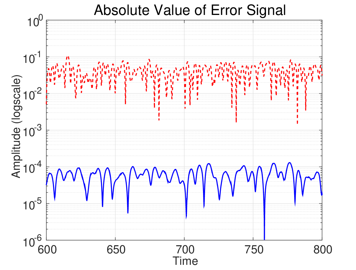
The dash-dot line represents by the canceller designed by a conventional method proposed in [5], and the solid line represents by the proposed canceller. This figure shows that the error is much reduced with the proposed method than with the conventional method. From this result, our method that takes account of the signal baseband subspace is much more effective than the conventional method.
VI Conclusion
In this article, we have proposed a new method for self-interference cancelation taking account of the baseband signal subspace. The problem is first formulated as a sampled-data control problem with a generalized sampler and a generalized hold, which can be reduced to a discrete-time -induced norm minimization problem. Taking account of the implementation of the generalized sampler and hold, we adopt the filter-sampler structure for the generalized sampler, and the uspampler-filter-hold structure for the generalized hold. Under these implementation constraints, we reformulate the problem as a standard discrete-time control problem by using the discrete-time lifting technique. A simulation result is shown to illustrate the effectiveness of the proposed method.
References
- [1] J. N. Laneman, D. N. C. Tse, and G. W. Wornell, “Cooperative diversity in wireless networks: Efficient protocols and outage behavior,” Information Theory, IEEE Transactions on, vol. 50, no. 12, pp. 3062–3080, 2004.
- [2] T. Cover and A. E. Gamal, “Capacity theorems for the relay channel,” Information Theory, IEEE Transactions on, vol. 25, no. 5, pp. 572–584, 1979.
- [3] ARIB 2020 and Beyond Ad Hoc Group, “White paper: mobile communications systems for 2020 and beyond,” 2014, (available at: http://www.arib.or.jp/english/20bah-wp-100.pdf).
- [4] M. Jain et al., “Practical, real-time, full duplex wireless,” in Proc. 17th Annual International Conference on Mobile Computing and Networking (MobiCom), 2011, pp. 301–312.
- [5] H. Sasahara, M. Nagahara, K. Hayashi, and Y. Yamamoto, “Digital cancelation of self-interference for single-frequency full-duplex relay stations via sampled-data control,” SICE Journal on Control, Measurement, and System Integration, 2015, (submitted, available at: http://arxiv.org/abs/1503.02379).
- [6] R. U. Nabar, H. Bolcskei, and F. W. Kneubuhler, “Fading relay channels: Performance limits and space-time signal design,” Selected Areas in Communications, IEEE Journal on, vol. 22, no. 6, pp. 1099–1109, 2004.
- [7] W. W. Jones and J. C. Dill, “The square root raised cosine wavelet and its relation to the meyer functions,” Signal Processing, IEEE Transactions on, vol. 49, no. 1, pp. 248–251, 2001.
- [8] Y. Yamamoto, From Vector Spaces to Function Spaces – Introduction to Functional Analysis with Applications. Society for Industrial and Applied Mathematics, 2012.
- [9] K. Gentile, “Digital pulse-shaping filter basics,” Analog Devices, Tech. Rep., 2007.
- [10] T. Chen and B. A. Francis, Optimal Sampled-Data Control Systems. Springer, 1995.
- [11] A. Goldsmith, Wireless Communications. Cambridge University Press, 2005.
- [12] W. H. Tranter, T. S. Rappaport, and K. L. Kosbar, Principles of Communication Systems Simulation with Wireless Applications. Prentice Hall, 2003.