Floer field theory for tanglesThanks: Partially supported by NSF grants CAREER 0844188 and DMS 0904358

Katrin Wehrheim Address: Department of Mathematics, University of California, Berkeley, Berkeley, CA 94720. E-mail address: katrin@math.berkeley.edu and Chris Woodward Address: Department of Mathematics, Rutgers University, Piscataway, NJ 08854. E-mail address: ctw@math.rutgers.edu

Abstract.

We use quilted Floer theory to construct functor-valued invariants of tangles arising from moduli spaces of flat bundles on punctured surfaces. As an application, we show the non-triviality of certain elements in the symplectic mapping class groups of moduli spaces of flat bundles on punctured spheres.

1. Introduction

In this paper we apply quilt theory in Lagrangian Floer cohomology, developed in Wehrheim-Woodward [51] and Ma’u-Wehrheim-Woodward [56], to produce functor-valued invariants of tangles via moduli spaces of flat bundles with traceless holonomies. In the gauge-theoretic interpretation of Jones polynomial provided by Witten [57], “quantizing” moduli spaces of flat bundles gives rise to knot invariants. In particular any tangle gives rise to a map between the spaces of quantum states by “quantization” of the corresponding Lagrangian correspondence. Several mathematicians and physicists (in particular Kronheimer-Mrowka [26] and Witten [58]) have investigated whether “categorifying” the moduli spaces of flat bundles lead to group-valued knot or tangle invariants. One naturally expects, according to a suggestion of Fukaya [9], that Lagrangian correspondences associated to tangles give rise to functors between Fukaya categories. The goal here is the modest one of constructing functor-valued invariants for tangles via Lagrangian Floer theory.

Our starting point is the observation that given a three-dimensional bordism containing a tangle whose components are labelled by conjugacy classes of a special unitary group, the set of flat bundles that extend over the bordism defines a formal Lagrangian correspondence

L(Y,K)\subset M(X_{-},\underline{x}_{-})\times M(X_{+},\underline{x}_{+})

between the moduli spaces $M(X_{\pm},\underline{x}_{\pm})$ of flat bundles associated to the incoming and outgoing marked, labelled boundary components. In good situations, our previous work [51] and work together with Ma’u [56] associates to such a correspondence a functor between the generalized Fukaya categories of the symplectic moduli spaces associated to the boundary components:

\Phi(L(Y,K)):{\operatorname{Fuk}^{\begin{picture}(0.0,-10.0)\end{picture}}}(M(X_{-},\underline{x}_{-}),w)\to{\operatorname{Fuk}^{\begin{picture}(0.0,-10.0)\end{picture}}}(M(X_{+},\underline{x}_{+}),w)

for any integer $w$ . Here ${\operatorname{Fuk}^{\begin{picture}(0.0,-10.0)\end{picture}}}(M,w)$ is the category whose objects are generalized simply-connected monotone Lagrangians submanifolds of a symplectic manifold $M$ with disk invariant $w$ , and morphisms are Floer cochains. The disk invariant $w$ is the number of Maslov two index disks passing through a generic point in the Lagrangian, see Definition 4.2 below.

One problem with this naive construction is that the moduli spaces of flat bundles over surfaces are in general not even smooth, let alone monotone as required for quilt invariants without Novikov coefficients or figure eight correction terms. We resolve this problem by making admissibility assumptions on the number of labels and conjugacy classes. By Proposition 3.6 and Theorem 3.10 this assumption guarantees smooth monotone symplectic manifolds. A second problem with the construction is that the Lagrangian correspondence is in general a singular subset of the product. To solve this we decompose the bordism into elementary bordisms-with-tangles

(Y,K)=(Y_{1},K_{1})\cup\ldots\cup(Y_{m},K_{m}).

as in Figure 1.

Refer to caption — Figure 1. Decomposition of a tangle (in this case, a knot) into elementary pieces

Each elementary piece $(Y_{i},K_{i})$ admits a Morse function with at most one critical point either on the bordism or the tangle. For such pieces the associated Lagrangian correspondences $L(Y_{i},K_{i})$ are smooth and even monotone. A decomposition into elementary bordisms-with-tangles is obtained by choosing a Morse function on the bordism such that the maxima resp. minima are the outgoing resp. incoming surfaces, and all critical points have different values. Then decomposition at level sets between the critical values yields a sequence of Lagrangian correspondences giving rise to our functor-valued invariant

\Phi(Y,K)=\Phi(L(Y_{m},K_{m}))\circ\ldots\circ\Phi(L(Y_{1},K_{1})).

A precise version of our main result is stated in the language of category-valued field theories. Given a compact oriented surface $X$ and coprime integers $r,d$ let $\operatorname{Tan}(X,r,d)$ denote the tangle category whose objects are finite oriented subsets $\underline{x}$ of $X$ with with admissible labels $\underline{\mu}$ as in Proposition 3.6, and whose morphisms are isotopy classes of tangles $K$ in $[-1,1]\times X$ .

Theorem 1.1.

(Floer field theory for tangles) Let $X$ be a compact oriented surface as above and $w$ an integer. There exists a functor from $\operatorname{Tan}(X,r,d)$ to the category of (small $A_{\infty}$ categories, homotopy classes of $A_{\infty}$ functors) that assigns to any finite subset $\underline{x}\subset X$ with labels $\underline{\mu}$ the generalized Fukaya category ${\operatorname{Fuk}^{\begin{picture}(0.0,-10.0)\end{picture}}}(M(X,\underline{x}),w)$ .

Gauge-theoretic invariants of knots were constructed using instantons by Collin-Steer [8] and Kronheimer-Mrowka [26]. See also Jacobsson-Rubinsztein [19] for the similarities with Khovanov homology. One expects the functors defined in this paper to be related to the instanton knot invariants by a version of the Atiyah-Floer conjecture.

The computation of these invariants is rather difficult since generators for the corresponding Fukaya categories are not presently known. However, one particular computation by Seidel [41] gives some information in the case of a five-punctured two-sphere with equal labels. In the last section we leverage Seidel’s computation to make a computation in the symplectic mapping class group

\operatorname{Map}(M(X,\underline{x}),\omega)=\pi_{0}(\operatorname{Diff}(M(X,\underline{x}),\omega))

of the moduli spaces of flat bundles:

Theorem 1.2.

(Non-triviality of twists on moduli spaces of bundles on punctured spheres) Let $X$ be a two-sphere and $\underline{x}\subset X$ an odd number of at least five marked points. Let $M(X,\underline{x})$ be the moduli space of flat $SU(2)$ -bundles with traceless holonomies on $X-\underline{x}$ and $\varphi:M(X,\underline{x})\to M(X,\underline{x})$ the symplectomorphism induced by a full twist around two markings. Then $\varphi$ is not Hamiltonian isotopic to the identity but is smoothly isotopic to the identity:

[\varphi]\neq[\operatorname{Id}]\in\operatorname{Map}(M(X,\underline{x}),\omega),\quad[\varphi]=[\operatorname{Id}]\in\operatorname{Map}(M(X,\underline{x})).

The structure of the paper is as follows. In Section 2 we describe our strategy for defining tangle invariants via Cerf decompositions. In Section 3 we then show that the moduli spaces of flat connections with admissible holonomy labels fit into this blueprint. In particular, the sequence of Lagrangian correspondences obtained as sketched above is independent of the choice of decomposition up to an equivalence relation generated by embedded composition of Lagrangian correspondences. In Section 4 we introduce a suitable notion of Fukaya category adapted to the moduli spaces of flat bundles under consideration. In Section 5 we combine the constructions of Sections 2,3,4 to obtain a category-valued field theory, or rather, a functor from our tangle categories to (small $A_{\infty}$ categories, homotopy classes of $A_{\infty}$ functors). The equivalence of generalized Lagrangian correspondences proved in Section 3 combines with the results of [51] to show that the resulting functor is independent up to isomorphism of the decomposition into elementary pieces. This section also contains an extension to graphs, needed for a surgery exact triangle.

We thank P. Seidel for encouragement and for sharing his ideas. We also thank R. Rezazadegan for helpful comments. The present paper is an updated and more detailed version of a paper the authors have circulated since 2007. The authors have unreconciled differences over the exposition in the paper, and explain their points of view at math.berkeley.edu/ $\sim$ katrin/wwpapers resp. christwoodwardmath.blogspot.com. The publication in the current form is the result of a mediation.

2. Field theory for tangles

In this section we introduce various notions and constructions of (topological) field theories for tangles. Roughly speaking a field theory is a functor from a bordism category to some other category. In Section 2.1 we use embedded bordisms in cylinders to construct a category of tangles. Section 2.2 discusses Cerf decompositions in this category and shows how to use them in the construction of general field theories. Section 2.3 then specializes this construction to a symplectic target category.

2.1. The tangle category

Our language for topological field theories for tangles adapts that in Lurie [29], rephrasing the earlier definition of Atiyah. Roughly speaking a tangle is a between marked surfaces, defined as follows.

Definition 2.1.

(a)

(Marked surfaces) A marking of a compact oriented surface $X$ is a collection

$\underline{x}=\{x_{1},\ldots,x_{n}\}\subset X$

of distinct, oriented points for some non-negative integer $n$ equipped with an orientation given by a function

$\epsilon:\underline{x}\to\{\pm 1\}.$

A marked surface is a tuple $(X,\underline{x})$ of a compact, oriented surface $X$ equipped with a marking $\underline{x}$ .
(b)
(Tangles) A tangle from $(X_{-},\underline{x}_{-})$ to $(X_{+},\underline{x}_{+})$ is a tuple $(Y,K,\phi)$ consisting of
1. (i)
  
  a compact oriented $3$ -manifold-with-boundary $Y$ ;
2. (ii)
  
  an orientation-preserving diffeomorphism $\phi:\partial Y\to\overline{X}_{-}\cup X_{+}$ where $\overline{X}_{-}$ denotes the manifold $X_{-}$ with reversed orientation;
3. (iii)
  
  a compact oriented $1$ -dimensional submanifold $K\subset Y$ meeting the boundary transversally in $\partial K=K\cap\partial Y$ , so that $\phi$ restricts to an orientation preserving identification
  
  $\phi|_{\partial K}:\ \partial K\cong{\underline{\overline{x}}_{-}}\cup\underline{x}_{+}$
  
  where ${\underline{\overline{x}}_{-}}$ denotes the marking $\underline{x}_{-}$ with reversed orientation.
An equivalence between two tangles $(Y_{0},K_{0},\phi_{0})$ and $(Y_{1},K_{1},\phi_{1})$ , both from $(X_{-},\underline{x}_{-})$ to $(X_{+},\underline{x}_{+})$ , is an orientation-preserving diffeomorphism inducing the identity on the boundary surfaces:

$\psi:Y_{0}\to Y_{1},\quad\psi(K_{0})=K_{1},\quad\phi_{1}\circ\psi|_{\partial Y_{0}}=\phi_{0}.$
(c)

(Labelled tangles) Let $\mathcal{B}$ be a set, which we call a set of labels. A decorated surface resp. tangle is a marked surface $(X,\underline{x})$ resp. tangle $(Y,K,\phi)$ equipped with a labelling of the components $\underline{x}\to\mathcal{B}$ resp. $\pi_{0}(K)\to\mathcal{B}$ .
(d)

(Cylindrical tangles) Let $X$ be a fixed compact, oriented $2$ -manifold. A $X$ -cylindrical tangle is a tangle in a bordism $Y$ from $X$ to itself diffeomorphic to $[-1,1]\times X$ .

Remark 2.2.

A weaker version of equivalence of tangles is isotopy invariance. In particular, suppose we fix a bordism $Y$ and suppose that $K_{t},t\in[0,1]$ is an isotopy of tangles in $Y$ with fixed endpoints. By a relative version of the isotopy extension theorem, whose absolute version is [18, Theorem 1.6, Chapter 8], the pairs $(Y,K_{t})$ are all diffeomorphic by diffeomorphism equal to the identity on the boundary; the relative version is proved in the way way as the absolute version. So $(Y,K_{t})$ are equivalent for $t\in[0,1]$ . The converse (that diffeomorphism equivalence implies isotopy equivalence) does not hold in general since the mapping class group of the pair could be non-trivial.

Our field theories fit into the language of topological field theories. These are functors from bordism categories equipped with additional data.

Definition 2.3.

(Tangle category) The tangle category $\operatorname{Tan}$ is the category whose

(a)

objects are marked surfaces;
(b)

morphisms are equivalence classes of tangles $[Y,K,\phi]$ ;
(c)

composition is defined by gluing: Let $(Y_{01},K_{01},\phi_{01})$ be a tangle from $(X_{0},\underline{x}_{0})$ to $(X_{1},\underline{x}_{1})$ and let $(Y_{12},K_{12},\phi_{12})$ be a tangle from $(X_{1},\underline{x}_{1})$ to $(X_{2},\underline{x}_{2})$ . Choose collar neighborhoods

$\kappa_{1}:(X_{1}\times(-\epsilon,0),\underline{x}_{1}\times(-\epsilon,0))\to(Y_{01},K_{01})$

resp.

$\kappa_{2}:(X_{1}\times(0,\epsilon),\underline{x}_{1}\times(0,\epsilon))\to(Y_{12},K_{12}).$

Define the composition $(Y_{01},K_{01},\phi_{01})\circ(Y_{12},K_{12},\phi_{12})$ to be the union

(1) $((Y_{01},K_{01})\sqcup(X_{1}\times(-\epsilon,\epsilon)\sqcup(Y_{12},K_{12}))/\sim$

where $\sim$ is the natural equivalence relation defined by $\kappa_{1},\kappa_{2}$ , and equipped with the diffeomorphism of the boundary to $(X_{0},\underline{x}_{0})\sqcup(X_{2},\underline{x}_{2})$ induced by $\phi_{01}$ and $\phi_{12}$ ;
(d)

the identity for $(X,\underline{x})$ is the equivalence class of the cylindrical bordism $\bigl[[-1,1]\times X,[-1,1]\times\underline{x}\bigr]$ equipped with the obvious identification of the boundary $\{-1,1\}\times(X,\underline{x})$ with two copies of $(X,\underline{x})$ .

Composition is independent, up to equivalence, of the choice of collar neighborhood and representatives, since any two collar neighborhoods are isotopic. The equivalence class of a composition of representatives is denoted

[(Y_{01},K_{01},\phi_{01})]\circ[(Y_{12},K_{12},\phi_{12})]=[(Y_{01},K_{01},\phi_{01})\circ(Y_{12},K_{12},\phi_{12})].

Equivalence classes of cylindrical tangles with fixed $X$ form a category $\operatorname{Tan}(X)$ by using the composition law described above, since the composition of two bordisms equivalent to $[-1,1]\times X$ is again equivalent to $[-1,1]\times X$ .

Definition 2.4.

(Field theories) Let $X$ be a compact oriented surface and let $\mathcal{C}$ be a category. A $\mathcal{C}$ -valued field theory for cylindrical tangles in $X$ is a functor $\Phi:\operatorname{Tan}(X)\to\mathcal{C}$ .

2.2. Cerf theory for tangles

Field theories for tangles can be constructed by decomposition into elementary tangles as follows.

Definition 2.5.

(a)

(Morse datum) A Morse datum for a tangle $(Y,K,\phi)$ from $(X_{-},\underline{x}_{-})$ to $(X_{+},\underline{x}_{+})$ consists of a pair $(f,\underline{b})$ of

(i)

a Morse function $f:Y\to\mathbb{R}$ that restricts to a Morse function $f|_{K}:K\to\mathbb{R}$ , and
(ii)

an ordered tuple $\underline{b}=(b_{0}<b_{1}<\ldots<b_{m})\in\mathbb{R}^{m+1}$

such that the following hold:

(i)

The sets of minima resp. maxima of $f$ are

$\phi(X_{-})\cong f^{-1}(b_{0}),\quad\phi(X_{+})\cong f^{-1}(b_{m}).$
(ii)

Each level set $f^{-1}(b)$ for $b\in\mathbb{R}$ is connected, or equivalently $f$ has no critical points of index $0$ or $3$ .
(iii)

The function $f$ has distinct values at the critical points of $f$ and $f|_{K}$ , i.e. it induces a bijection

${\operatorname{Crit}}(f)\cup{\operatorname{Crit}}(f|_{K})\to f({\operatorname{Crit}}(f)\cup{\operatorname{Crit}}(f|_{K}))$

between critical points and critical values.

(iv)

The values $b_{0},\ldots,b_{m}\in\mathbb{R}\setminus f({\operatorname{Crit}}(f)\cup{\operatorname{Crit}}(f|_{K}))$ are regular values of $f$ and $f|_{K}$ such that each interval $(b_{i-1},b_{i})$ contains at most one critical value of either $f$ or $f|_{K}$ :

\#{\operatorname{Crit}}(f)\cap f^{-1}(b_{i-1},b_{i})+\#{\operatorname{Crit}}(f_{K})\cap f^{-1}(b_{i-1},b_{i})\leq 1.

In the special case $Y=[b_{-},b_{+}]\times X$ , we say that $(f,\underline{b})$ is a cylindrical Morse datum for a tangle $(Y,K,\phi)$ if

\partial_{t}f(t,x)>0,\quad\forall(t,x)\in Y.

This assumption implies that each level set $f^{-1}(t)$ is diffeomorphic to $X$ , by normalized gradient flow of $f$ .

(b)

(Cerf decomposition) The Cerf decomposition of a tangle $(Y,K,\phi)$ induced by a Morse datum $(f,\underline{b})$ is the sequence

(Y_{i}:=f^{-1}([b_{i-1},b_{i}]),\quad K_{i}:=Y_{i}\cap K,\phi_{i}),\quad i=1,\ldots m

of elementary tangles between the connected level sets

X_{i}:=Y_{i}\cap Y_{i+1}=f^{-1}(b_{i}),\quad\underline{x}_{i}=K_{i}\cap K_{i+1}=f^{-1}(b_{i})\cap K

and obvious identifications of the boundary $\phi_{i}$ . Here we have $X_{0}\cong X_{-}$ and $X_{m}\cong X_{+}$ via the restriction of $\phi$ , $\partial Y_{i}=X_{i-1}\sqcup X_{i}$ . The sequence $(Y_{i},K_{i},\phi_{i})_{i=1,\ldots m}$ corresponds to the decomposition

(2)

Y=Y_{1}\cup_{X_{1}}Y_{2}\cup_{X_{2}}\ldots\cup_{X_{m-1}}Y_{m},\ \ \ K=K_{1}\cup_{\underline{x}_{1}}K_{2}\cup_{\underline{x}_{2}}\ldots\cup_{\underline{x}_{m-1}}K_{m}.

In the special case $Y=[b_{-},b_{+}]\times X$ , a cylindrical Cerf decomposition of the tangle $K$ is a Cerf decomposition induced by a cylindrical Morse datum.

(c)

(Elementary tangles) A tangle $(Y,K,\phi)$ is a

(i)

elementary tangle if $(Y,K,\phi)$ admits a Cerf decomposition with a single piece, and
(ii)

an elementary cylindrical tangle if $(Y,K,\phi)$ admits a Cerf decomposition with a single piece and no critical points on $Y$ . That is, $Y$ is a cylindrical bordism and $f:Y\to\mathbb{R}$ is a Morse function without critical points and the restriction $f|K$ has at most one critical point on $K$ :

$\#{\operatorname{Crit}}(f)=0,\quad\#{\operatorname{Crit}}(f_{K})\leq 1.$

Thus a cylindrical Cerf decomposition is a decomposition of the trivial bordism $Y=[b_{-},b_{+}]\times X$ into cylindrical bordisms $Y_{1}\cup_{X_{1}}\ldots\cup_{X_{m-1}}Y_{m}$ , with the property that taking intersections with the tangle gives a decomposition $K=K_{1}\cup_{\underline{x_{1}}}\ldots\cup_{\underline{x}_{m-1}}K_{m}$ into elementary cylindrical tangles $(Y_{j},K_{j},\phi_{j})$ . The equivalence class $[(Y_{j},K_{j},\phi_{j})]$ of an elementary tangle $(Y_{j},K_{j},\phi_{j})$ is an elementary morphism. An cylindrical Cerf decomposition of an equivalence class $[(Y,K,\phi)]$ is an expression as a composition of elementary morphisms

[(Y,K,\phi)]=[(Y_{1},K_{1},\phi_{1})]\circ\ldots\circ[(Y_{m},K_{m},\phi_{m})]

corresponding to a cylindrical Cerf decomposition of a representative. We say that two cylindrical Cerf decompositions

	$\displaystyle[(Y,K,\phi)]$	$\displaystyle=$	$\displaystyle[(Y_{1},K_{1},\phi_{1})]\circ\ldots\circ[(Y_{m},K_{m},\phi_{m})]$
		$\displaystyle=$	$\displaystyle[(Y_{1},K_{1},\phi_{1})^{\prime}]\circ\ldots\circ[(Y_{m},K_{m},\phi_{m})^{\prime}]$

are equivalent if there exist orientation-preserving diffeomorphisms

\delta_{0}=\operatorname{Id}_{X_{0}},\quad\delta_{1}:X_{1}\to X_{1}^{\prime},\quad\ldots\quad,\delta_{m-1}:X_{m-1}\to X_{m-1}^{\prime},\quad\delta_{m}=\operatorname{Id}_{X_{m}}

such that for each $i=1,\ldots,m$ ,

[(Y_{i},K_{i},\phi_{i})]=[(Y_{i}^{\prime},K_{i}^{\prime},(\delta_{i-1}\sqcup\delta_{i})\circ\phi_{i})].

The following is a special case of Cerf theory, for the special case of cylindrical Cerf decompositions.

Theorem 2.6.

(Cerf theory for tangles) Let $(Y=[-1,1]\times X,K,\phi)$ be a cylindrical tangle. Then any two cylindrical Cerf decompositions of $[(Y,K,\phi)]$ are related up to equivalence by a finite sequence of the following moves:

(a)

(Critical point cancellation) Two elementary morphisms $[(Y_{i},K_{i},\phi_{i})]$ and $[(Y_{i+1},K_{i+1},\phi_{i+1})]$ , that carry Morse functions $f_{i}$ resp. $f_{i+1}$ with a local minimum $y_{i}\in K_{i}$ resp. local maximum $y_{i+1}\in K_{i+1}$ ,

${\mbox{d}}^{2}_{y_{i}}f|_{K_{i}}>0,\quad d^{2}_{y_{i+1}}f|_{K_{i+1}}<0$

both of which lie on the same strand of $K\cap(Y_{i}\cup Y_{i+1})$ , are replaced by the elementary morphism $[(Y_{i},K_{i},\phi_{i})]\circ[(Y_{i+1},K_{i+1},\phi_{i+1})]$ that admits a Morse function with no critical point;

(b)

(Critical point reversal) Two elementary morphisms $[(Y_{i},K_{i},\phi_{i})],[(Y_{i+1},K_{i+1},\phi_{i+1})]$ that carry Morse functions with critical points

y_{i}\in K_{i},\ y_{i+1}\in K_{i+1},\quad{\mbox{d}}_{y_{i}}f={\mbox{d}}_{y_{i+1}}f=0,\quad k=\operatorname{ind}(y_{i}),\quad l=\operatorname{ind}(y_{i+1})

on strands whose intersection with $(X_{i},\underline{x}_{i})$ is disjoint, are replaced by two elementary morphisms that carry Morse functions with critical points of index $l$ and $k$ such that $[(Y_{i},K_{i},\phi_{i})]\circ[(Y_{i+1},K_{i+1},\phi_{i+1})]$ is equal to $[(Y_{i}^{\prime},K_{i}^{\prime},\phi_{i}^{\prime})]\circ[(Y_{i+1}^{\prime},K_{i+1}^{\prime},\phi_{i+1}^{\prime})]$

(c)

(Cylinder gluing) Two elementary morphisms $[(Y_{i},K_{i},\phi_{i})],[(Y_{i+1},K_{i+1},\phi_{i+1})]$ , one of which is cylindrical, are replaced by the composition $[(Y_{i},K_{i},\phi_{i})]\circ[(Y_{i+1},K_{i+1},\phi_{i+1})]$ .

See Figures 2 and 3 for depictions of the first two moves.

Figure 2. Critical point cancellation

Proof.

The proof follows from an examination of a generic homotopy between cylindrical Morse functions defining the two Cerf decompositions. Let $(f_{j},\underline{b}_{j}),j=0,1$ be cylindrical Morse data for a cylindrical tangle $(Y,K,\phi)$ . Let

f_{s}=(1-s)f_{0}+sf_{1},s\in[0,1]

be the linear interpolation between $f_{0}$ and $f_{1}$ . Since $\partial_{t}f_{0}>0$ and $\partial_{t}f_{1}>0$ we also have $\partial_{t}f_{s}>0$ for all $s\in[0,1]$ . Consider the restrictions $f_{s}|_{K}$ . Since $K\subset[b_{-},b_{+}]\times X$ is a submanifold with boundary, $f_{s}|_{K}$ has positive resp. negative normal derivative at $\underline{x}_{-}$ resp. $\underline{x}_{+}$ . Hence $(f_{s}|_{K})$ has singularities or critical points only on a compact set in the interior of $K$ .

Next we apply Cerf theory to the restriction of the homotopy to the tangle. After replacing $f_{s}|_{K}$ with a perturbation we may assume that $f_{s}|_{K}$ is Morse except at finitely many values of $s\in[0,1]$ where a birth/death singularity occurs by [14, Theorem 2.4]. Furthermore, after another perturbation we may assume that $f_{s}|_{K}$ is a Morse function injective on its critical set for all but finitely many values of $s\in[0,1]$ , as in Cerf [7, top of p. 11]. Since $K$ is a submanifold of $Y$ , any such perturbation has an extension to a smooth family of functions $f_{s}$ on $Y$ with the property that $\partial_{t}f_{s}>0$ for all $(t,x)\in Y$ and $s\in[0,1]$ . So this homotopy has only finite many values $c_{1}<\ldots<c_{m}$ for which $f_{c_{j}}$ does not satisfy (a-c) in Definition 2.6.

Away from the critical values the Cerf decompositions are equivalent by diffeomorphisms. Indeed, choose $\epsilon$ small and smoothly varying $b_{1}(s),\ldots,b_{m-1}(s)$ separating the critical values of $f_{s}$ for $s\in[c_{i}+\epsilon,c_{i+1}-\epsilon]$ . Let $\tilde{f}(s,t)=f_{s}(t)$ . The inverse images of the level sets $f_{s}^{-1}(b_{i}(s))$ form smooth submanifolds of $Y\times[0,1]$ denoted $\tilde{f}^{-1}(b_{i})$ . Indeed, the differential of $f_{s}$ is already transverse to $b_{i}(s)$ , so smoothness follows from the implicit function theorem. The required diffeomorphism will be given by the flow of a vector field satisfying

v\in\operatorname{Vect}(Y\times[c_{i}+\epsilon,c_{i+1}-\epsilon]),\quad(D_{y,s}\pi_{2})_{*}v=\partial_{s},\forall(y,s)\in Y\times[c_{i}+\epsilon,c_{i+1}-\epsilon]

where $\pi_{2}$ is projection onto the second factor, and tangent to the boundary components and tangles:

v(K)\subset TK,\quad v(\tilde{f}^{-1}(b_{i}))\subset T(\tilde{f}^{-1}(b_{i})).

The construction of the required vector field proceeds in stages. Such a vector field $v$ exists on each level set $\tilde{f}^{-1}(b_{i})$ since the $b_{i}(s)$ are regular values:

T_{y,s}\tilde{f}^{-1}(b_{i})\cap(T_{y}Y\times\{0\})=T_{y}f^{-1}(b_{i}(s)),\quad D\pi_{2}|T_{y,s}\tilde{f}^{-1}(b_{i})=\mathbb{R}.

Furthermore since $K\cap\tilde{f}^{-1}(b_{i})$ is a transverse intersection, we may choose $v$ preserving $K\cap\tilde{f}^{-1}(b_{i})$ . Next $v$ extends to a vector field $v|_{U_{i}}$ on a neighborhood $U_{i}$ of each level set $\tilde{f}^{-1}(b_{i})$ by the tubular neighborhood theorem. One may then extend $v$ to a vector field on $Y\times[c_{i}+\epsilon,c_{i+1}-\epsilon])$ using interpolation with the vector field $\partial_{s}\in\operatorname{Vect}(Y\times[c_{i}+\epsilon,c_{i+1}-\epsilon])$ . That is, let $\rho\in C^{\infty}(Y\times[c_{i}+\epsilon,c_{i+1}-\epsilon])$ be a bump function equal to one on a neighborhood of $\tilde{f}^{-1}(b_{i})$ . Set

(3)

v=\rho v|_{U_{i}}+(1-\rho)\partial_{s}\in\operatorname{Vect}(Y\times[c_{i}+\epsilon,c_{i+1}-\epsilon]).

The flow of $v$ preserves the level sets $\tilde{f}^{-1}(b_{i})$ as well as the tangles $K$ and so defines diffeomorphisms of the pieces of the Cerf decomposition of $(Y,K)$ for $f_{s}$ . Hence the functions ${f}_{s}$ for $s\in[c_{i}+\epsilon,c_{i+1}-\epsilon]$ define equivalent Cerf decompositions of $[(Y,K,\phi)]$ .

It remains to consider the relationship between the Cerf decompositions for small values on either side of time at which a crossing or birth-death occurs. The Cerf decompositions are equivalent for all but one or two pieces by the same argument in the previous paragraph. For those pieces, one either has a critical point switch move or critical point cancellation by the local model for the cusp singularities [55, p.157] for the restriction of $\tilde{f}$ to $K$ . ∎

Figure 3. Critical point reversal

By Theorem 2.6, in order to construct field theories for cylindrical tangles it suffices to construct the theory on elementary tangles and check that the Cerf moves are satisfied.

Theorem 2.7.

(Field theories for tangles via elementary tangles) Let $\mathcal{C}$ be a category and $X$ a compact oriented surface. Suppose there is given a partially defined functor $\Phi$ from $\operatorname{Tan}(X)$ to $\mathcal{C}$ that associates

(a)

to each marking $\underline{x}$ of $X$ , an object $\Phi(\underline{x})$ of $\mathcal{C}$ ;
(b)

to each equivalence class of elementary cylindrical tangles $(Y,K,\phi)$ from $(X,\underline{x}_{-})$ to $(X,\underline{x}_{+})$ , a morphism $\Phi([(Y,K,\phi)])$ from $\Phi(\underline{x}_{-})$ to $\Phi(\underline{x}_{+})$ ;

and satisfies the following Cerf relations:

(a)

If $(Y,K,\phi)=([-1,1]\times X,[-1,1]\times\underline{x},\phi)$ is a trivial tangle, then $\Phi([(Y,K,\phi)])$ is the identity.

(b)

If $(Y_{1},K_{1},\phi_{1})$ from $\underline{x}_{0}$ to $\underline{x}_{1}$ and $(Y_{2},K_{2},\phi_{2})$ from $\underline{x}_{1}$ to $\underline{x}_{2}$ are composable elementary cylindrical tangles such that $[(Y_{1},K_{1},\phi_{1})]\circ[(Y_{2},K_{2},\phi_{2})]$ is equivalent to a cylindrical tangle via critical point cancellation, then

\Phi([(Y_{1},K_{1},\phi_{1})])\circ\Phi([(Y_{2},K_{2},\phi_{2})])=\Phi([(Y_{1},K_{1},\phi_{1})\circ(Y_{2},K_{2},\phi_{2})]);

(c)

If $(Y_{1},K_{1},\phi_{1}),(Y_{2},K_{2},\phi_{2})$ and $(Y_{1}^{\prime},K_{1}^{\prime},\phi_{1}^{\prime}),(Y_{2}^{\prime},K_{2}^{\prime},\phi_{2}^{\prime})$ are elementary cylindrical tangles related by critical point reversal, then

\Phi([(Y_{1},K_{1},\phi_{1})])\circ\Phi([(Y_{2},K_{2},\phi_{2})])=\Phi([(Y_{1}^{\prime},K_{1}^{\prime},\phi_{1}^{\prime})])\circ\Phi([(Y_{2}^{\prime},K_{2}^{\prime},\phi_{2}^{\prime})]);

(d)

If $(Y_{1},K_{1},\phi_{1}),(Y_{2},K_{2},\phi_{2})$ are composable elementary tangles, one of which is cylindrical, then

\Phi([(Y_{1},K_{1},\phi_{1})])\circ\Phi([(Y_{2},K_{2},\phi_{2})])=\Phi([(Y_{1},K_{1},\phi_{1})]\circ[(Y_{2},K_{2},\phi_{2})])

then there is a unique $\mathcal{C}$ -valued field theory extending $\Phi$ .

In other words, to define a field theory for tangles it suffices to define the morphisms for elementary bordisms and prove the Cerf relations.

2.3. Symplectic-valued field theories

In this section we specialize to field theories with values in the symplectic category. A symplectic-valued field theory for tangles in particular assigns to any tangle a sequence of Lagrangian correspondences, up to equivalence, as in [51].

Definition 2.8.

(Geometric composition of Lagrangian correspondences) Let $M_{j}$ be symplectic manifolds with symplectic forms $\omega_{M_{j}}$ for $j=0,1,2$ .

(a)

A Lagrangian correspondence from $M_{1}$ to $M_{2}$ is a Lagrangian submanifold $L\subset M_{1}^{-}\times M_{2}$ with respect to the symplectic structure $-\omega_{M_{1}}\oplus\omega_{M_{2}}$ .

(b)

The geometric composition of Lagrangian correspondences

L_{01}\subset M_{0}^{-}\times M_{1},\quad L_{12}\subset M_{1}^{-}\times M_{2}

is the point set

(4)

L_{01}\circ L_{12}:=\pi_{M_{0}\times M_{2}}\bigl((L_{01}\times L_{12})\cap(M_{0}\times\Delta_{M_{1}}\times M_{2})\bigr)\subset M_{0}\times M_{2}.

(c)

A geometric composition is called transverse if the intersection in (4) is transverse (and hence smooth). The geometric composition is embedded if, in addition, the restriction of the projection $\pi_{M_{0}\times M_{2}}$ is an injection of the smooth intersection, hence an embedding. In that case the image is a smooth Lagrangian correspondence $L_{01}\circ L_{12}\subset M_{0}^{-}\times M_{2}$ .

Definition 2.9.

(a)
(Generalized correspondences) Let $M_{-},M_{+}$ be symplectic manifolds. A generalized Lagrangian correspondence $\underline{L}$ from $M_{-}$ to $M_{+}$ consists of
1. (i)
  
  a sequence $N_{0},\ldots,N_{r}$ of any length $r\geq 0$ of symplectic manifolds with $N_{0}=M_{-}$ and $N_{r}=M_{+}$ , and
2. (ii)
  
  a sequence $L_{01},\ldots,L_{(r-1)r}$ of compact Lagrangian correspondences with $L_{(j-1)j}\subset N_{j-1}^{-}\times N_{j}$ for $j=1,\ldots,r$ .

(b)

(Algebraic composition) Let $M,M^{\prime},M^{\prime\prime}$ be symplectic manifolds. The algebraic composition of generalized Lagrangian correspondences $\underline{L}$ from $M$ to $M^{\prime}$ and $\underline{L}^{\prime}$ from $M^{\prime}$ to $M^{\prime\prime}$ is given by concatenation

\underline{L}{\begin{picture}(0.0,-10.0)\end{picture}}\underline{L}^{\prime}:=(L_{01},\ldots,L_{(m-1)m},L_{1}^{\prime},\ldots,L_{(m^{\prime}-1)m^{\prime}}^{\prime}).

(c)

(Symplectic category) The symplectic category $\operatorname{Symp}$ is the category defined as follows.

(i)

Objects are smooth compact symplectic manifolds.
(ii)

Morphisms from an object $M_{-}$ to an object $M_{+}$ are generalized Lagrangian correspondences from $M_{-}$ to $M_{+}$ modulo the composition equivalence relation $\sim$ generated by

(5) $\bigl(\ldots,L_{(j-1)j},L_{j(j+1)},\ldots\bigr)\sim\bigl(\ldots,L_{(j-1)j}\circ L_{j(j+1)},\ldots\bigr)$

for all sequences and $j$ such that $L_{(j-1)j}\circ L_{j(j+1)}$ is transverse and embedded. We also set the empty sequence $\emptyset$ to be equivalent to the diagonal $\Delta_{M}\subset M^{-}\times M$ .

(iii)

Composition of morphisms

[\underline{L}]\in\operatorname{Hom}(M,M^{\prime}),\quad[\underline{L}^{\prime}]\in\operatorname{Hom}(M^{\prime},M^{\prime\prime})

for symplectic manifolds $M,M^{\prime},M^{\prime\prime}$ is defined by

[\underline{L}]\circ[\underline{L}^{\prime}]:=[\underline{L}{\begin{picture}(0.0,-10.0)\end{picture}}\underline{L}^{\prime}]\;\in\operatorname{Hom}(M,M^{\prime\prime});

(iv)

The identity $1_{M}\in\operatorname{Hom}(M,M)$ is the equivalence class of the empty sequence $1_{M}=\emptyset$ of length zero. The identity $1_{M}$ is also the equivalence class $1_{M}:=[\Delta_{M}]$ of the diagonal. Indeed, the sequence of any number of diagonals $\Delta_{M}\subset M^{-}\times M$ is equivalent to the empty set:

$\emptyset\sim(\Delta_{M})\sim(\Delta_{M},\Delta_{M})\sim\ldots.$

(d)

(Monotone symplectic manifolds and correspondences) A symplectic manifold $(M,\omega)$ is monotone with monotonicity constant $\tau>0$ if the symplectic class is positively proportional to the first Chern class: $\tau c_{1}(M)=[\omega]$ in $H^{2}(M)$ . A Lagrangian submanifold $L\subset M$ is monotone if

$2\int u^{*}\omega=\tau I(u),\quad\forall u:(D,\partial D)\to(M,L)$

where $I(u)$ is the Maslov index. A generalized Lagrangian correspondence $\underline{L}=(L_{01},\ldots,L_{(r-1)r})$ is monotone if every components $L_{j(j-1)}$ is a Lagrangian correspondence.
(e)

(Monotone symplectic category) For $\tau>0$ denote by $\operatorname{Symp}_{\tau}$ the category whose objects are monotone symplectic manifolds $M$ with monotonicity constant $\tau$ and morphisms from $M_{-}$ to $M_{+}$ are equivalence classes of simply-connected¹¹ 1 For convenience; alternatively one can impose further monotonicity conditions. generalized Lagrangian correspondences $\underline{L}$ from $M_{-}$ to $M_{+}$ whose components are compact oriented monotone equipped with relative spin structures.
(f)

A symplectic-valued field theory for cylindrical tangles resp. monotone symplectic-valued field theory for cylindrical tangles for a compact oriented surface $X$ is a functor $\Phi:\operatorname{Tan}(X)\to\operatorname{Symp}\ \text{resp.}\quad\Phi:\operatorname{Tan}(X)\to\operatorname{Symp}_{\tau}.$

3. Flat bundles on complements of tangles

In this section we construct a symplectic-valued field theory for a particular class of labelled tangle categories. For suitable choices of the labels, this field theory will be monotone. The basic construction is well-known: associated to any tangle there is a moduli space of flat bundles with fixed holonomies around the components. If smooth and embedded this moduli space defines a Lagrangian correspondence in the moduli spaces of flat bundles with fixed holonomies on the boundary. For elementary tangles, the correspondences are smooth and embedded, and we check that the Cerf relations hold.

3.1. Moduli spaces via holonomy

We choose to describe the moduli spaces via representations of the fundamental group, rather than gauge theory as in [53]. We begin with some Lie-theoretic notation for the special unitary group.

Definition 3.1.

Let $r\geq 2$ and $G=SU(r)$ the group of special unitary $r\times r$ matrices. We identify the Lie algebra $\mathfrak{g}=\mathfrak{su}(r)$ with traceless skew-Hermitian $r\times r$ matrices.

(a)

(Weyl alcove) The Weyl alcove for $SU(r)$ is the subset

\mathfrak{A}=\left\{(\lambda_{1}\leq\ldots\leq\lambda_{r})\in\mathbb{R}^{r}\ \left|\ \sum_{i=1}^{r}\lambda_{i}=0,\lambda_{r}-\lambda_{1}\leq 1\right.\right\}.

A point $\mu\in\mathfrak{A}$ will be called a label. The alcove $\mathfrak{A}$ embeds as a subset of the Lie algebra $\mathfrak{g}$ via the diagonal map,

\mathfrak{A}\to\mathfrak{g},\quad(\mu_{1},\ldots,\mu_{r})\to\operatorname{diag}(\mu_{1},\ldots,\mu_{r}).

(b)

(Conjugacy classes for the special unitary group) Conjugacy classes in $SU(r)$ are parametrized by the Weyl alcove via

$\mathcal{C}_{\mu}=\{g\exp(\operatorname{diag}(2\pi i\mu))g^{-1}\ |\ g\in SU(r)\},\quad\mu\in\mathfrak{A}.$

Each conjugacy class

(6) $\mathcal{C}_{\mu}\cong SU(r)/S(U(m_{1})\times\ldots U(m_{k}))$

is diffeomorphic to the quotient of $SU(r)$ by a centralizer subgroup isomorphic to $S(U(m_{1})\times\ldots U(m_{k}))$ where $m_{i},i=1,\dots,k$ are the multiplicities of the eigenvalues. Thus each $\mathcal{C}_{\mu}$ is diffeomorphic to a partial flag variety. This implies that $\mathcal{C}_{\mu}$ is simply connected.

(c)

(Involution) Taking inverses defines a (possibly trivial) involution of the alcove

(7)

*:\mathfrak{A}\to\mathfrak{A},\ (\lambda_{1},\ldots,\lambda_{r})\mapsto(-\lambda_{r},\ldots,-\lambda_{1}),\quad\mathcal{C}_{*\mu}=\mathcal{C}_{\mu}^{-1}.

(d)

(Vertices) Let

\omega_{k}=(\underbrace{(r-k)/r,\ldots,(r-k)/r}_{k},\underbrace{-k/r,\ldots,-k/r}_{r-k}),\quad 1\leq k\leq r-1,\quad\omega_{0}=0

denote the vertices of $\mathfrak{A}$ .

(e)

(Barycenter) Let

$\rho=(-r+1,-r-3,\ldots,r-3,r-1)/2$

denote the barycenter of the re-scaled alcove $r\mathfrak{A}$ . The vector $\rho$ is the unique vector with components $\rho_{i}$ satisfying

$\rho_{i+1}-\rho_{i}=1,\ i=0,\ldots,r-1,\quad\rho_{r}-\rho_{1}=r-1.$

The element $\rho/r$ is the barycenter of $\mathfrak{A}$ .

Next we introduce notation for manifolds of flat bundles with fixed holonomies. We define these via representations of the fundamental group.

Definition 3.2.

(a)

(Loops around strands) Let $X$ be a compact, connected, oriented manifold, possibly with boundary. Let $K\subset X$ be an oriented, embedded submanifold of codimension $2$ . Let $K_{1},\ldots,K_{n}$ denote the connected components of $K$ . Let

$\gamma_{j}:S^{1}\to X\setminus K,\quad j=1,\ldots,n$

be small loops around $K_{j}$ , so that the induced orientation on the normal bundle of $K_{j}$ agrees with that induced by the orientations of $K_{j}$ and $X$ . Each $\gamma_{j}$ defines a conjugacy class $[\gamma_{j}]\subset\pi_{1}(X\setminus K)$ of loops obtained by joining $\gamma_{j}$ to a base point. We implicitly fix a base point in the definition of the fundamental group $\pi_{1}(X\setminus K)$ .

(b)

(Moduli of flat bundles with fixed holonomies) For labels $\underline{\mu}=(\mu_{1},\ldots,\mu_{n})\in\mathfrak{A}^{n}$ let $M(X,K)$ denote the moduli space of flat $G$ -bundles on $X\kern-2.15277pt\smallsetminus\kern-2.15277ptK$ whose holonomy around $\gamma_{j}$ lies in the conjugacy class $\mathcal{C}_{\mu_{j}}$ . We call the element $\mu_{j}$ the label of the component $K_{j}$ . The moduli space $M(X,K)$ of connections with fixed holonomy has a description in terms of representations of the fundamental group, that we take as a definition:

(8)

M(X,K):=\bigl\{\varphi\in\operatorname{Hom}(\pi_{1}(X\kern-2.15277pt\smallsetminus\kern-2.15277ptK),G))\,\big|\,\varphi([\gamma_{j}])\subset\mathcal{C}_{\mu_{j}}\forall j\bigr\}/G.

Here $G$ acts by conjugation so that $(g\varphi)([\gamma])=g\varphi([\gamma])g^{-1}.$ In case $X$ is not connected, say the union of connected components $X_{1},\ldots,X_{k}$ , this definition is replaced by the product of moduli spaces for the connected components of $X$ ,

M(X,K)=M(X_{1},K\cap X_{1})\times\ldots\times M(X_{k},K\cap X_{k}).

Remark 3.3.

(Effect of orientation change of the tangle) Changing the orientation of a component $K_{j}$ (i.e. of $\gamma_{j}$ ) corresponds to changing the label $\mu_{j}$ by the involution $*$ of the alcove $\mathfrak{A}$ in (7). That is, if $\tilde{K}$ denotes the tangle obtained by changing the orientation on $K_{j}$ and $\tilde{\underline{\mu}}$ is the set of labels obtained by replacing $\mu_{j}$ with $*\mu_{j}$ then there is a canonical homeomorphism $M(X,K)\to M(X,\tilde{K})$ .

Remark 3.4.

(Alternative description in the finite-order case) Suppose that the conjugacy classes $\mathcal{C}_{\underline{\mu}}=\mathcal{C}_{\mu_{1}}\times\ldots\times\mathcal{C}_{\mu_{n}}$ each have finite order as in all our examples, so that

\exists k_{1},\ldots,k_{n}\in\mathbb{Z},\quad g_{i}^{k_{i}}=e,\quad\forall g_{i}\in\mathcal{C}_{\mu_{i}},i=1,\ldots,n.

In this case one can identify the moduli space $M(X,K)$ with the moduli space of flat bundles on an orbibundle over $X$ , see [32, 25, 33] for two- and four-dimensional cases. However, we will avoid using the equivariant description via gauge theory. Instead we check explicitly, in specific presentations, the smoothness of those moduli spaces that enter our constructions.

3.2. Moduli spaces of bundles for surfaces

The key feature of moduli spaces of bundles on compact, oriented surfaces is their symplectic nature. Below we review the description of the symplectic structure in the holonomy description.

Remark 3.5.

Let $X$ be a compact, connected, oriented surface of genus $g$ , and let $\underline{x}=\{x_{1},\ldots,x_{n}\}$ be a marking.

(a)

(Presentation of the fundamental group) Recall that $\epsilon_{j}=\pm 1$ depending on whether the orientation of $x_{j}$ agrees with the standard orientation of a point. The fundamental group $\pi_{1}(X\kern-2.15277pt\smallsetminus\kern-2.15277pt\underline{x})$ has standard presentation

\pi_{1}(X\kern-2.15277pt\smallsetminus\kern-2.15277pt\underline{x})\cong\big\langle\;\alpha_{1},\ldots,\alpha_{2g},\gamma_{1},\ldots,\gamma_{n}\ |\ \Pi_{j=1}^{g}[\alpha_{2j},\alpha_{2j+1}]\Pi_{j=1}^{n}\gamma_{j}^{\epsilon_{j}}=1\;\big\rangle,

where $\gamma_{j}$ is a loop around $x_{j}$ , oriented corresponding to $\epsilon_{j}$ .

(b)

(Presentation of the moduli space of flat bundles) Let $\underline{\mu}\in\mathfrak{A}^{n}$ be a set of labels for $\underline{x}$ . The moduli space of flat $G$ -bundles with fixed holonomy can be described in terms of a standard presentation of $\pi_{1}(X\setminus\underline{x})$ by

	$\displaystyle M(X,\underline{x})$	$\displaystyle=\bigl\{\varphi\in\operatorname{Hom}(\pi_{1}(X\kern-2.15277pt\smallsetminus\kern-2.15277pt\underline{x}),G))\,\big\|\,\varphi([\gamma_{j}])\subset\mathcal{C}_{\mu_{j}}\forall j\bigr\}/G$
(9)			$\displaystyle\cong\bigl\{(\underline{a},\underline{b})\in G^{2g}\times\mathcal{C}_{\underline{\mu}}\ \|\ \Phi(\underline{a},\underline{b})=1\bigr\}/G,$

where $G$ acts on $G^{2g}\times\mathcal{C}_{\underline{\mu}}$ diagonally by conjugation and

(10)

\Phi((a_{1},\ldots,a_{2g}),(b_{1},\ldots,b_{n}))=\prod_{j=1}^{g}[a_{2j},a_{2j+1}]\prod_{j=1}^{n}b_{j}^{\epsilon_{j}}.

(c)

(Symplectic form on the moduli space) For any $X,\underline{x},\underline{\mu}$ the space $M(X,\underline{x})$ can be realized as the moduli space of flat connections on the trivial $G$ -bundle over $X\kern-2.15277pt\smallsetminus\kern-2.15277pt\underline{x}$ with fixed holonomies around $\underline{x}$ (see [32, 33]) and as such has a symplectic form. The form can be described explicitly in the holonomy description [2] as follows.

First we recall the symplectic structure on the moduli space in the case of a surface without markings. Let $\theta,\overline{\theta}\in\Omega^{1}(G,\mathfrak{g})$ be the left and right-invariant Maurer-Cartan forms, defined so that

\theta_{e}(\xi)=\xi,\quad\overline{\theta}_{e}(\xi)=\xi,\quad\forall\xi\in\mathfrak{g}\cong T_{e}G.

Define a form $\omega_{1}$ on $G^{2}$ by

\omega_{1}\in\Omega^{2}(G^{2}),\ \ \ \ \omega_{1}=\langle l^{*}\theta\wedge r^{*}\overline{\theta}\rangle/2+\langle l^{*}\overline{\theta}\wedge r^{*}\theta\rangle/2

where $l,r:G^{2}\to G$ are the projections on the first and second factor. For $g\geq 1$ define two-forms $\omega_{g}\in\Omega^{2}(G^{2g})$ inductively by

(11)

\omega_{g}=\omega_{g_{1}}+\omega_{g_{2}}+\langle\Phi_{g_{1}}^{*}\theta\wedge\Phi_{g_{2}}^{*}\overline{\theta}\rangle/2

where $g=g_{1}+g_{2}$ is any splitting with $g_{1},g_{2}\geq 1$ ,

\Phi_{g_{j}}:(G^{2})^{g_{j}}\to G,\quad(a_{1},\ldots,a_{2g_{j}})\mapsto\prod_{j=1}^{g_{j}}[a_{2j},a_{2j+1}]

is the product of commutators. We omit pull-backs to the factors of $G^{2g}\cong G^{2g_{1}}\times G^{2g_{2}}$ from the notation to save space. A theorem of Alekseev-Malkin-Meinrenken [2, Theorem 9.3], extending earlier work of Weinstein, Jeffrey, and Karshon, states that the restriction of $\omega_{g}$ to the identity level set of $\Phi_{g}$ descends to the symplectic form on the locus of irreducible representations in $M(X,\underline{x})$ .

Next we define the symplectic structure for a marked surface. For any label $\mu\in\mathfrak{A}$ , define a $2$ -form $\omega_{\mu}$ on the conjugacy class $\mathcal{C}_{\mu}$ by

\omega_{\mu}(v_{\xi}(g),v_{\eta}(g))=\langle\theta(v_{\eta}(g))+\overline{\theta}(v_{\eta}(g)),\xi\rangle,\ \ \ g\in\mathcal{C}_{\mu},\ \ \ \ \xi,\eta\in\mathfrak{g}

where $v_{\xi},v_{\eta}\in\operatorname{Vect}(\mathcal{C}_{\mu})$ are the generating vector fields for $\xi,\eta$ . Define two-forms $\omega_{g,\underline{\mu}}\in\Omega^{2}(G^{2g}\times\mathcal{C}_{\underline{\mu}})$ inductively as follows. First, set

\omega_{g,\emptyset}=\omega_{g},\quad\omega_{0,\{\mu\}}=\omega_{\mu}.

For any splitting $g=g_{1}+g_{2},\underline{\mu}=\underline{\mu}_{1}\cup\underline{\mu}_{2}$ , where for each $j=1,2$ either $g_{j}>0$ or $\underline{\mu}_{j}$ is non-empty, set

(12)

\omega_{g,\underline{\mu}}=\omega_{g_{1},\underline{\mu}_{1}}+\omega_{g_{2},\underline{\mu}_{2}}+\langle\Phi_{g_{1},\underline{\mu}_{1}}^{*}\theta\wedge\Phi_{g_{2},\underline{\mu}_{2}}^{*}\overline{\theta}\rangle/2

where

\Phi_{g_{j},\underline{\mu}_{j}}:G^{2g_{j}}\times\mathcal{C}_{\underline{\mu}_{j}}\to G,\ \ \ \ (\underline{h},(c_{\mu})_{\mu\in\underline{\mu}_{j}})\mapsto\Phi_{g_{j}}(\underline{h})\prod_{\mu\in\underline{\mu}_{j}}c_{\mu}.

By [2, page 27], the restriction of $\omega_{g,\underline{\mu}}$ to the identity level set of $\Phi_{g,\underline{\mu}}$ descends to the symplectic form on the locus of irreducible representations in $M(X,\underline{x})$ .

In case $X$ is not connected, we define $M(X,\underline{x})$ to be the product of moduli spaces for its connected components.

In order to construct Floer theory we wish for our moduli spaces to be smooth. The next result is a sufficient condition.

Proposition 3.6.

(Sufficient conditions for smoothness) Let $(X,\underline{x})$ be a marked surface of genus $g$ with $n$ labels $\underline{\mu}$ . Suppose that each label is half of a vertex, and the sum of labels satisfies a parity condition:

(13)

\{\mu_{i},i\in\{1,\ldots,n\}\}\subset\{\omega_{j}/2,j\in\{1,\ldots,r\}\},\quad 2\sum_{i=1}^{n}\mu_{i}=\omega_{d}\ \ \text{mod}\ \Lambda

for some $d$ coprime to $r$ . Then $M(X,\underline{x})$ is a smooth compact symplectic manifold and we call the labels $\underline{\mu}$ admissible.

Proof.

Recall the description of the moduli space of flat bundles as a group-valued symplectic quotient from [2]. Let $\mathcal{C}_{\underline{\mu}}$ denote the corresponding product of conjugacy classes $\mathcal{C}_{\mu_{j}},j=1,\ldots,n$ . The space $M(X,\underline{x})$ can be realized as a symplectic quotient of the group-valued Hamiltonian $G$ -manifold $\widetilde{M}(X,\underline{x}):=G^{2g}\times\mathcal{C}_{{\underline{\mu}}}$ with group-valued moment map $\Phi:\widetilde{M}(X,\underline{x})\to G$ given by the product (9). The identity level set of the moment map is cut out transversally if and only if all stabilizers are discrete, by [2, Definition 2.2,Condition B3]. For each tuple $w=(w_{1},\ldots,w_{n})\in W^{n}$ and subset $I\subset\{1,\ldots,l\}$ such that the span of $(\alpha_{i})_{i\in I}$ is not all of $\mathfrak{t}^{\vee}\cong\mathfrak{t}$ , define the wall corresponding to $w$ by

\Theta_{w,I}:=\exp\Bigl(\textstyle{\sum_{j=1}^{n}}w_{j}\mu_{j}+\operatorname{span}(\alpha_{i})_{i\in I}\Bigr).

Let $T^{X,\operatorname{sing}}$ denote the singular values of $\Phi$ contained in $T$ . We claim that the set of singular values is contained in the union of walls:

T^{X,\operatorname{sing}}\subseteq\cup_{w,I}\Theta_{w,I}.

Any orbit stratum in $\mathcal{C}_{\mu_{j}}$ with infinite stabilizer group contains a $T$ -fixed point in its closure, since the same is true for coadjoint orbits by equivariant formality of Hamiltonian actions [15, Appendix C]. Similarly, the closure of any orbit stratum in $G^{2g}$ with infinite stabilizer is equal to $H^{2g}$ , for some subgroup $H$ containing $T$ up to conjugacy. Now $T^{2g}$ maps to the identity under the product of commutators $\Phi$ . Putting everything together, any orbit-type stratum $Y$ in $\widetilde{M}(X,\underline{x})$ contains a $T$ -fixed point $y$ in its closure. The image of such a fixed point $y$ under the group-valued moment map satisfies

\Phi(y)\in\exp\left(\sum_{j=1}^{n}w_{j}\mu_{j}\right)

for some $w\in W^{n}$ , since the commutators of elements in the maximal torus vanish. The tangent space $T_{y}Y$ is a sum of root spaces, and the assumption that the stabilizer of $Y$ is infinite implies that the span of the roots appearing in the sum is not all of $\mathfrak{t}^{\vee}$ . It follows that the moduli space is an orbifold if for each tuple $w_{1},\ldots,w_{n}\in W$ we have

(14)

\langle{\textstyle\sum_{i=1}^{n}}w_{i}\mu_{i},\omega_{j}\rangle\notin\langle\Lambda,\omega_{j}\rangle\qquad\forall j=1,\ldots,r

where $\Lambda=\exp^{-1}(1)$ is the coweight lattice. Now suppose that each $\mu_{i}$ is equal to $\frac{1}{2}\omega_{j}$ for some $j\in\{1,\ldots,r\}$ , and

2\sum_{i=1}^{n}\mu_{i}=\omega_{d}\ \ \text{mod}\ \Lambda

as in (13). Since each $\langle\mu_{j},\alpha_{k}\rangle$ is a half-integer and the Weyl group is generated by simple reflections we have $\sum w_{i}\mu_{i}-\sum\mu_{i}\in\Lambda$ . From the relation

\omega_{d}=(d/r)(\alpha_{1}+2\alpha_{2}+\ldots+d\alpha_{d})+((r-d)/r)((r-d)\alpha_{d+1}+\ldots+\alpha_{r-1})

it follows that the pairing

\langle\omega_{d}/2,\omega_{j}\rangle=(d/2r)\langle j\alpha_{j},\omega_{j}\rangle=jd/2r\ \text{mod}\ \mathbb{Z}

is never an integer for $r$ coprime to $d$ and $j=1,\ldots,r-1$ . This implies (14).

It remains to show that the moduli spaces of flat bundles are in fact manifolds. The centralizer subgroups in the unitary group are connected, being the maximal compact subgroup of the centralizers in the general linear group. The latter are the intersections of subspaces with matrices of non-zero determinant, and so connected. It follows that the centralizer subgroups in the projectivized unitary group are also connected. Hence the moduli spaces are quotients of smooth manifolds by the free action of the projectivized unitary group, and so are manifolds. ∎

Proposition 3.7.

(Admissibility on one end implies admissibility on the other) Suppose that $K\subset Y=[-1,1]\times X$ is a tangle from $X_{-}=\{-1\}\times X$ to $X_{+}=\{+1\}\times X$ , such that each label is half of a vertex of the alcove, and the labels for $X_{-}\cap K$ are admissible in the sense of (13). Then the same hold for the induced labels of $X_{+}\cap K$ .

Proof.

The labels on $X_{\pm}$ are the same except for labels that have disappeared due to critical points of index $1$ and those that have appeared due to critical points of index $0$ . By assumption the labels of two strands meeting in this way are opposite up to conjugacy and so do not contribute to the sum in (13). ∎

Sufficient conditions for monotonicity of the moduli space are provided by Meinrenken-Woodward [34]. The condition is a discrete condition on the set of labels, although in special cases the set of monotone labels may be larger and non-discrete.

Definition 3.8.

(Monotone labels) A label $\mu\in\mathfrak{A}$ is monotone if $\mu$ is a projection of the Coxeter element onto a face $\sigma$ of the Weyl alcove, that is,

\exists\sigma\subset\mathfrak{A},\quad\mu=\operatorname{proj}_{\sigma}(\rho/r)

where $\operatorname{proj}_{\sigma}$ denotes orthogonal projection onto $\sigma$ .

Example 3.9.

(Examples of monotone labels)

(a)

(Rank two case) If $G=SU(2)$ , then $c=2$ then we identify $\mathfrak{A}\cong[0,{1/2}]$ by the map $(\lambda,-\lambda)\mapsto\lambda$ . The conjugacy class $\mathcal{C}_{\mu}$ consists of matrices with eigenvalues $\exp(\pm 2\pi i\mu)$ . We have $\rho={1/2}$ . If $\mu={1/4}$ , $\mathcal{C}_{\mu}$ consists of all traceless matrices. The monotone elements are $0$ , ${1/2}$ , ${1/4}\in\mathfrak{A}$ .
(b)

(Rank three case) If $G=SU(3)$ , the alcove $\mathfrak{A}$ is the convex hull of the vectors $(0,0,0),(2/3,-1/3,-1/3)$ and $(1/3,1/3,-2/3)$ . We have $\rho=(1,0,-1)$ . See Figure 4 for the monotone labels.

Theorem 3.10.

(Sufficient conditions for monotonicity, [34, Theorem 4.2]) Let $(X,\underline{x})$ be a marked surface with labels $\underline{\mu}$ . If each label $\mu_{j}$ is monotone and $M(X,\underline{x})$ is smooth then $M(X,\underline{x})$ is monotone with monotonicity constant $\tau^{-1}=2r$ .

Finally we note that the natural action of the diffeomorphism group acts by symplectomorphisms:

Definition 3.11.

(Marking-preserving mapping class group) Let $\operatorname{Diff}_{+}(X,\underline{x})$ be the subgroup of orientation-preserving diffeomorphisms $\varphi\in\operatorname{Diff}_{+}(X)$ that preserve the marked points, orientations, and labels:

(15)

\operatorname{Diff}_{+}(X,\underline{x})=\left\{\varphi\in\operatorname{Diff}_{+}(X)\,\big|\,\varphi(\underline{x})=\underline{x},\ \varphi^{*}\underline{\epsilon}=\underline{\epsilon},\ \varphi^{*}\underline{\mu}=\underline{\mu}\right\}.

Here we denote the maps

\underline{\epsilon}:\underline{x}\to\{\pm 1\},x_{i}\mapsto\epsilon_{i},\quad\underline{\mu}:\underline{x}\to\mathfrak{A},x_{i}\mapsto\mu_{i}.

So the conditions in (15) are

(\varphi(x_{i})=x_{j})\implies(\epsilon_{i}=\epsilon_{j}\ \text{and}\ \mu_{i}=\mu_{j}),\quad\forall i,j=1,\ldots,n.

Let $\operatorname{Map}_{+}(X,\underline{x})$ be the quotient of $\operatorname{Diff}_{+}(X,\underline{x})$ by isotopy.

Remark 3.12.

(Spherical braid group action) The action of $\operatorname{Map}_{+}(X,\underline{x})$ on $\pi_{1}(X\kern-2.15277pt\smallsetminus\kern-2.15277pt\underline{x})$ induces an action on $M(X,\underline{x})$ by symplectomorphisms on the smooth stratum. See for example [2, Section 9.4] for a proof from the holonomy point of view. In particular, if $X$ is a sphere and all labels are equal, $\underline{\mu}=(\mu,\ldots,\mu)$ , then the spherical braid group $\operatorname{Map}_{+}(X,\underline{x})$ acts on $M(X,\underline{x})$ . Explicitly let $\sigma_{i(i+1)}\in\operatorname{Map}_{+}(X,\underline{x})$ is the half-twist of $x_{i}$ and $x_{i+1}$ . For suitable choice of presentation of $\pi_{1}(X\kern-2.15277pt\smallsetminus\kern-2.15277pt\underline{x})$ we have

(16)

\sigma_{i(i+1)}:M(X,\underline{x})\to M(X,\underline{x}),\\ \quad[b_{1},\ldots,b_{n}]\mapsto[b_{1},\ldots,b_{i-1},b_{i+1},b_{i+1}^{-1}b_{i}b_{i+1},b_{i+2},\ldots,b_{n}].

3.3. Moduli spaces for tangles

Given a tangle we construct Lagrangian correspondences as follows.

Definition 3.13.

Let $(Y,K,\phi)$ be a labelled tangle from $(X_{-},\underline{x}_{-})$ to $(X_{+},\underline{x}_{+})$ .

(a)

(Restriction to the boundary) Let $K_{1},\ldots,K_{p}$ be the connected components of $K$ and fix labels $\underline{\nu}=(\nu_{1},\ldots,\nu_{p})\in\mathfrak{A}^{p}$ for $K$ . In Section 3.1 we defined the moduli space $M(Y,K)$ of flat $G$ -bundles on $Y\kern-2.15277pt\smallsetminus\kern-2.15277ptK$ with holonomy around $K_{j}$ in $\mathcal{C}_{\nu_{j}}$ . On the boundary the labels $\underline{\nu}$ induce labels $\underline{\mu}_{\pm}\in\mathfrak{A}^{n_{\pm}}$ defined by $\nu_{j}$ for $\partial K_{j}$ . Restriction to the boundary and pull-back under $\phi$ define a map

(17) $M(Y,K)\to M(X_{-},\underline{x}_{-})^{-}\times M(X_{+},\underline{x}_{+}).$

More precisely, the inclusion of the boundary and a choice of paths between base points induces a map of fundamental groups

$\pi_{1}(X_{-})\sqcup\pi_{1}(X_{+})\to\pi_{1}(Y)$

that is well-defined up to conjugacy. The dual maps the representation variety of the bordism to the product of representation varieties of its boundary components, independent of the choice of path.
(b)

(Correspondences for tangles) For any labelled tangle $(Y,K,\phi)$ we denote the image of (17) by

$L(Y,K,\phi)\subset M(X_{-},\underline{x}_{-})^{-}\times M(X_{+},\underline{x}_{+}).$

Lemma 3.14.

(Correspondences for compositions) Let $(X_{i},\underline{x}_{i})$ be marked surfaces for $i=0,1,2$ , and let $(Y_{01},K_{01},\phi_{01})$ resp. $(Y_{12},K_{12},\phi_{12})$ be tangle from $(X_{0},\underline{x}_{0})$ to $(X_{1},\underline{x}_{1})$ resp. from $(X_{1},\underline{x}_{1})$ to $(X_{2},\underline{x}_{2})$ . Let $\underline{\nu}_{01}$ and $\underline{\nu}_{12}$ be labels for the bordisms with tangles such that they induce the same label $\underline{\mu}_{1}$ for $(X_{1},\underline{x}_{1})$ . Gluing provides a bordism with tangle $(Y_{01}\circ Y_{12},K_{01}\circ K_{12})$ from $(X_{0},\underline{x}_{0})$ to $(X_{2},\underline{x}_{2})$ with labels $\underline{\nu}_{01}\circ\underline{\nu}_{12}$ . The induced labels $\underline{\mu}_{0}$ for $\underline{x}_{0}$ and $\underline{\mu}_{2}$ for $\underline{x}_{2}$ are the same as the ones induced from $\underline{\nu}_{01}$ and $\underline{\nu}_{12}$ , and we have the equality of subsets of $M(X_{0},\underline{x}_{0},\underline{\mu}_{0})\times M(X_{2},\underline{x}_{2},\underline{\mu}_{2})$

L((Y_{01},K_{01},\phi_{01})\circ(Y_{12},K_{12},\phi_{12}))=L(Y_{01},K_{01},\phi_{01})\circ L(Y_{12},K_{12},\phi_{12}).

Proof.

By the Seifert-van Kampen theorem we have an isomorphism (using a base point on $X_{1}$ )

\pi_{1}(Y_{01}\circ Y_{12}\setminus K_{01}\circ K_{12})\cong\pi_{1}(Y_{01}\setminus K_{01})\star_{\pi_{1}(X_{1}\setminus\underline{x}_{1})}\pi_{1}(Y_{12}\setminus K_{12}).

In particular, any representation $\varphi:\pi_{1}(Y_{01}\circ Y_{12}\setminus K_{01}\circ K_{12})\to G$ induces representations on both sides $\varphi_{j(j+1)}:{\pi_{1}(Y_{j(j+1)}\setminus K_{j(j+1)})}\to G,j=0,1$ , whose restriction to $X_{1}\setminus\underline{x}_{1}$ agree. Conversely, any pair of representations on the two sides, whose restrictions to $X_{1}\setminus\underline{x}_{1}$ are conjugate, we can conjugate one of the sides so that the restrictions agree. Patching induces a representation on the glued space. ∎

Lemma 3.15.

(Correspondences for elementary tangles)

(a)

(Cylindrical bordisms) Suppose that $(Y,K,\phi)$ admits a surjective Morse function $f:Y\to[-1,1]$ with no critical points on $Y$ or $K$ . The map $f:Y\to[-1,1]$ is a fiber bundle containing $K$ that admits a simultaneous trivialization

{\mathcal{T}}:([-1,1]\times X_{-},[-1,1]\times\underline{x}_{-})\to(Y,K),

where

{\mathcal{T}}|_{f^{-1}(-1)}={\rm Id}_{X_{-}},\quad\psi:=\phi\circ{\mathcal{T}}|_{f^{-1}(1)}:(X_{-},\underline{x}_{-})\to(X_{+},\underline{x}_{+})

are isomorphisms of marked surfaces. The correspondence associated to $(Y,K,\phi)$ is then the graph:

L(Y,K,\phi)=\operatorname{graph}((\psi^{-1})^{*})\subset M(X_{-},\underline{x}_{-})^{-}\times M(X_{+},\underline{x}_{+}).

(b)

(Elementary tangles) Let $X$ be a compact oriented surface, $Y=[-1,1]\times X$ the trivial bordism and suppose that $Y$ admits a cylindrical Morse function such that $K$ contains a single critical point that is a maximum, and so consists of $n-2$ strands meeting both the incoming and outgoing boundary, and one strand that connects two incoming markings $x_{i},x_{j}$ , as in Figure 5. The map $L(Y,K,\phi)\to M(X,\underline{x}_{+})$ induced by pullback is a coisotropic embedding, and $L(Y,K,\phi)\to M(X,\underline{x}_{-})$ is a fiber bundle with fiber $\mathcal{C}_{\mu_{i}}\cong\mathcal{C}_{\mu_{j}}$ .
(c)

(Quilted cups and caps) More generally, suppose that $X$ be a compact oriented surface and $Y=[-1,1]\times X$ a product bordism. Suppose that $Y$ admits a cylindrical Morse function such that all critical points in $K$ have the same index. Then the pull-back map $L(Y,K,\phi)\to M(X,\underline{x}_{+})$ is a coisotropic embedding and $L(Y,K,\phi)\to M(X_{-},\underline{x}_{-})$ is a fiber bundle with fiber a product of conjugacy classes.
(d)

(Elementary bordisms) Suppose that $Y$ admits a Morse function with a single critical point of index $1$ . The map $\pi_{+}$ from $L(Y,K,\phi)$ to $M(X_{+},\underline{x}_{+})$ is a coisotropic embedding, and the map $\pi_{-}$ from $L(Y,K,\phi)$ to $M(X_{-},\underline{x}_{-})$ is a fiber bundle with fiber $G$ .

Furthermore, in each case $L(Y,K,\phi)$ is a smooth Lagrangian correspondence in $M(X_{-},\underline{x}_{-})^{-}\times M(X_{+},\underline{x}_{+}).$

Figure 5. A cup

Proof.

(a) First we construct a simultaneous trivialization. Suppose that $(Y,K,\phi)$ admits a Morse function $f:Y\to[-1,1]$ with no critical points on $Y$ or $K$ . Choose a vector field $v$ on $K$ with flow $\psi_{t}$ so that that $\frac{d}{dt}f\circ\psi_{t}=1$ ; for example, a normalized gradient vector field. Via the patching procedure in (3), the vector field $v$ extends to all of $Y$ to a vector field $v\in\operatorname{Vect}(Y)$ with $L_{v}f>0$ . After normalizing, we may assume $L_{v}f=1$ in which case the flow ${\mathcal{T}}(x_{-},-1+t)=\psi_{t}(x_{-})$ gives the claimed trivialization.

Next we identify the correspondence associated to the bordism as a graph of a symplectomorphism. With notation from the previous paragraph any representation $\rho^{\prime}$ of $\pi_{1}(Y\setminus K)$ is the pullback $({\mathcal{T}}^{-1})^{*}\rho$ of a representation $\rho$ of the trivial cylinder over $X_{-}\setminus\underline{x}_{-}$ . Since the restrictions of $\rho$ to the two boundary components are conjugate, the boundary restriction of $({\mathcal{T}}^{-1})^{*}\rho$ will be the graph of pullback under $\psi^{-1}=(\phi\circ{\mathcal{T}})^{-1}|_{X_{+}}:X_{+}\to X_{-}$ . Moreover, $\psi^{-1}$ preserves the orientations and labels and hence induces a symplectomorphism of moduli spaces $M(X_{-},\underline{x}_{-})\to M(X_{+},\underline{x}_{+})$ . So $L(Y,K,\phi)$ is the graph of a symplectomorphism and hence a smooth Lagrangian correspondence.

Next we consider the case (b) of an elementary tangle. Choose a system of generators of the fundamental groups of the punctured surfaces such that in the holonomy description

	$\displaystyle L(Y,K,\phi)$	$\displaystyle=\bigl\{\bigl([a_{1},\ldots,a_{2g},h_{1},\ldots,h_{n+2}],$
		$\displaystyle\qquad\quad[a_{1},\ldots,a_{2g},h_{1},\ldots,\hat{h}_{i},\ldots,\hat{h}_{j},\ldots,h_{n+2}]\bigr)\,\big\|\,h_{i}=h_{j}\bigr\}.$

Such a system of generators can be found as follows. Let $k_{0}\in K$ denote the unique critical point, by assumption a maximum. Choose

b_{+}:=f(X_{+})>c_{+}>f(k_{0})>c_{-}>f(X_{-})=:b_{-}

such that the bordisms $f^{-1}([b_{-},c_{-}])$ and $f^{-1}([b_{+},c_{+}])$ are cylindrical. Any choice of generators for the fundamental groups of $f^{-1}(c_{\pm})$ induces generators for the fundamental groups of $f^{-1}(b_{\pm})$ . Consider the bordism $f^{-1}([c_{-},c_{+}])$ . For $c_{\pm}$ sufficiently close to $f(k_{0})$ , the level set $f^{-1}(c_{+})$ is obtained from $f^{-1}(c_{-})$ by replacing a twice punctured disk $D_{-}$ by a disk $D_{+}$ without punctures:

f^{-1}(c_{+})=f^{-1}(c_{-})-D_{-}\cup D_{+}.

The two punctures labelled $i,j$ in $D_{-}$ are connected in $f^{-1}([c_{-},c_{+}])$ by a small cap. Choose a system of representatives for generators for $\pi_{1}(f^{-1}(c_{-}))$ that except for the generators $\gamma_{i},\gamma_{j}$ around the $i$ -th and $j$ -th markings do not meet $D_{-}$ . Removing the two generators $\gamma_{i},\gamma_{j}$ produces a system of generators for $f^{-1}(c_{+})$ . Since the $i$ -th and $j$ -st strands are connected by a cap, the holonomies around the punctures $x_{i},x_{j}\in X_{+}$ are inverses, up to conjugacy. By (7) we have $\mu_{i}=*\mu_{j}$ .

The presentation above implies that the Lagrangian correspondence is smooth. Indeed, since $M(X_{-},\underline{x}_{-})$ is a smooth quotient, the level sets

\prod_{j=1}^{g}[a_{2j},a_{2j+1}]\prod_{k\neq i,j}h_{k}^{\epsilon_{k}}=1,\quad h_{i}=h_{j}

are transversally cut out. Thus $L(Y,K)$ is the free quotient of a smooth manifold by the projectivized unitary group, and so smooth. The map $\pi_{-}:L(Y,K,\phi)\to M(X_{-},\underline{x}_{-})$ is the identity on the holonomies not around $x_{i},x_{j}$ , and so is a smooth fibration. Using the identification $\mathcal{C}_{\mu_{j}}\to\mathcal{C}_{*\mu_{i}},g\mapsto g^{-1}$ the fiber may be identified with the antidiagonal

\Delta_{i}:=\{(h,h^{-1})\,|\,h\in\mathcal{C}_{\mu_{i}}\}\subseteq\mathcal{C}_{\mu_{i}}\times\mathcal{C}_{*\mu_{i}}.

The symplectic form on $M(X_{+},\underline{x}_{+})$ is given by reduction from the 2-form (12) on $G^{2g}\times\mathcal{C}_{\underline{\mu}_{+}}\cong G^{2g}\times\mathcal{C}_{\underline{\mu}_{-}}\times\mathcal{C}_{\mu_{i}}\times\mathcal{C}_{*\mu_{i}}$ . In the latter splitting the 2-form is

(18)

\omega_{g,\underline{\mu}_{-}}+\omega_{0,\{\mu_{i},*\mu_{i}\}}+\langle\Phi_{g,\underline{\mu}_{-}}^{*}\theta\wedge\Phi_{0,\{\mu_{i},*\mu_{i}\}}^{*}\overline{\theta}\rangle/2.

The second and third term vanish on $G^{2g}\times\mathcal{C}_{\underline{\mu}_{-}}\times\Delta_{i}$ . The same holds after taking quotients. Hence the fibers of the projection $L(Y,K,\phi)$ to $M(X_{-},\underline{x}_{-})$ are isotropic, and the projection to $M(X_{-},\underline{x}_{-})$ is a coisotropic embedding. Cases (c) and (d) are similar. ∎

Corollary 3.16.

(Lagrangian correspondences for elementary tangles) If $(Y,K,\phi)$ is a elementary tangle as in Definition 2.5 from $(X_{-},\underline{x}_{-})$ to $(X_{+},\underline{x}_{+})$ and the labels $\underline{\nu}$ for the components of $K$ are such that the moduli spaces $M(X_{\pm},\underline{x}_{\pm})$ are smooth manifolds (see Proposition 3.6) then the moduli space $L(Y,K,\phi)$ is a smooth Lagrangian correspondence from $M(X_{-},\underline{x}_{-})$ to $M(X_{+},\underline{x}_{+})$ .

Proof.

There are three cases to consider, depending on whether a critical point occurs in the tangle, so that $\#{\operatorname{Crit}}(f|K)\geq 1$ ; in the ambient bordism, so that $\#{\operatorname{Crit}}(f)\geq 1$ ; or not at all, so that $\#{\operatorname{Crit}}(f)=\#{\operatorname{Crit}}(f_{K})=0.$ In the first case, the critical point must be a maximum or minimum. Up to symmetry, this is exactly the setting of Lemma 3.15 (b), so the claim follows. For a critical point in the ambient bordism the index of the critical point must be either one or two; up to symmetry this is Lemma 3.15 (c). The third case follows from Lemma 3.15 (a). ∎

Remark 3.17.

Relative spin structures will be needed later to provide orientations on moduli spaces of holomorphic quilts. Recall from [10], [54] that a relative spin structure with background class $b\in H^{2}(M;\mathbb{Z}_{2})$ is a trivialization of $TL\oplus E_{b}|L$ over the $2$ -skeleton of $L$ with respect to some triangulation, where $E_{b}\to M$ is an orientable rank two bundle with $w_{2}(E_{b})=b$ . Two relative spin structures are equivalent mod $w_{2}(TM)$ if their background classes are related by $b-b^{\prime}=w_{2}(TM)$ , that is, by adding Stiefel-Whitney classes $w_{2}(TM)\in H^{2}(M,\mathbb{Z}_{2})$ , and the corresponding trivializations of $L\oplus E_{b}$ are related by adding the canonical trivialization of $TM|L$ on the $2$ -skeleton.

Remark 3.18.

(Background classes for moduli of bundles) Suppose that $\underline{x}_{i}$ consists of $n_{i}^{\pm}$ markings with positive resp. negative orientation, and $\mu_{i}^{\pm}$ are the labels of the points with positive resp. negative orientation. We take as background classes for $M(X_{i},\underline{x}_{i})$ the Stiefel-Whitney classes for conjugacy classes associated to the positively or negatively oriented markings

(19)

b_{\pm}(X_{i},\underline{x}_{i}):=w_{2}(T(\Pi_{j=1}^{n_{i}^{\pm}}\mathcal{C}_{\mu_{i}^{\pm}})/\kern-3.01385pt/G)\in H^{2}(M(X_{i},\underline{x}_{i}),\mathbb{Z}_{2}).

Here $T(\Pi_{j=1}^{n_{i}^{\pm}}\mathcal{C}_{\mu_{i}^{\pm}})/\kern-3.01385pt/G$ denotes the bundle obtained by pulling back $T(\Pi_{j=1}^{n_{i}^{\pm}}\mathcal{C}_{\mu_{i}^{\pm}})$ to $G^{2g}\times\mathcal{C}_{\underline{\mu}}$ , restricting to $\Phi^{-1}(e)$ , and quotienting by the action of $G$ . The classes $b_{\pm}(X_{i},\underline{x}_{i})$ are equivalent modulo $w_{2}(TM(X_{i},\underline{x}_{i}))$ , since $G$ is equivariantly spin.

Lemma 3.19.

(Relative spin structures) Let $(Y,K,\phi)$ be an oriented elementary tangle from $(X_{-},\underline{x}_{-})$ to $(X_{+},\underline{x}_{+})$ so that $X_{+}\cong X_{-}$ and $\underline{x}_{+}$ has at least as many elements as $\underline{x}_{-}$ . Let $\underline{\nu}$ be a labelling of $K$ such that the moduli spaces $M(X_{\pm},\underline{x}_{\pm})$ are smooth manifolds. Then $L(Y,K,\phi)$ is simply-connected, so oriented. There is a unique relative spin structure on $L(Y,K,\phi)$ with background class $(b_{\pm}(X_{-},\underline{x}_{-}),b_{\mp}(X_{+},\underline{x}_{+}))$ of (19). These relative spin structures are compatible under composition in the sense that the relative spin structures on $L(Y_{01},K_{01})\circ L(Y_{12},K_{12})$ and $L(Y_{02},K_{02})$ agree up to shifts by $w_{2}(TM(X_{i},\underline{x}_{i}))$ .

Proof.

It suffices to consider the case of a single critical point, since the case of no critical points is trivial. Suppose first that $K$ contains a critical point of index $0$ , with a strand connecting the markings $x_{i},x_{j}\in X_{+}$ . Suppose that the orientation of $x_{j}$ resp. $x_{i}$ is the same resp. opposite of the standard orientation of a point. By Lemma 3.15, $L(Y,K,\phi)$ is diffeomorphic to a $\mathcal{C}_{\mu_{j}}$ -bundle over $M(X_{-},\underline{x}_{-}).$ The base $M(X_{-},\underline{x}_{-})$ is simply-connected because $M(X_{-},\underline{x}_{-})$ is homeomorphic to the moduli space of parabolic bundles [32] and the moduli space of parabolic bundles is simply-connected [36]. The conjugacy classes of $G$ are simply-connected, since they are partial flag varieties. Hence $L(Y,K,\phi)$ is simply connected as well.

An orientation on the Lagrangian correspondence is defined as follows. Since the base $M(X_{-},\underline{x}_{-})$ is simply-connected and the structure group of the bundle $SU(r)$ is connected, an orientation $L(Y,K,\phi)$ is induced by the symplectic orientation on the base $M(X_{-},\underline{x}_{-})$ and the orientation on the fiber $\mathcal{C}_{\mu_{j}}$ .

Relative spin structures are defined as follows. By the assumption on the size of $\underline{x}_{+}$ the map $L(Y,K,\phi)\to M(X_{+},\underline{x}_{+})$ is an embedding. The Lagrangian $L(Y,K,\phi)$ is a quotient of the diagonal $h_{i}=h_{j}$ for some $i,j$ with the same labels $\underline{\nu}$ except for the singe label $\nu_{k}:=\mu_{+,i}=\mu_{+,j}$ labelling the unique strand that connects $X_{+}$ to itself. The inclusion

G^{2g}\times\mathcal{C}_{\underline{\nu}}\to(G^{2g}\times\mathcal{C}_{\underline{\mu}_{-}})\times(G^{2g}\times\mathcal{C}_{\underline{\mu}_{+}})

has an equivariant relative spin structure with background class (19), since each conjugacy class embeds into a diagonal and exactly one of each pair of conjugacy classes appears in (19). Taking quotients one obtains a relative spin structure on $L(Y,K,\phi)$ . Since $L(Y,K,\phi)$ is simply connected, this relative spin structure is unique for this background class. Compatibility under composition follows from uniqueness. ∎

3.4. Symplectic-valued field theory

Putting everything together we construct a functor from the tangle category to the category of (symplectic manifolds, equivalence classes of generalized Lagrangian correspondences.) We denote by

\mathcal{B}=\{\omega_{1}/2,\ldots,\omega_{r}/2\}

the set of midpoints on the edges connecting the origin with the vertices in the Weyl alcove, and restrict to marked surfaces with labels in this set. For example, in the rank two case this assumption means that all labels are contained in the set $\mathcal{B}=\{{1/4}\}\subset[0,{1/2}]\cong\mathfrak{A}$ corresponding to traceless holonomies.

Definition 3.20.

(Admissible tangle category) Fix coprime integers $r,d>0$ . Let $X$ be a compact oriented surface. Denote by $\operatorname{Tan}(X,r,d)$ the category of cylindrical whose objects are markings in $X$ with labels in $\mathcal{B}$ such that the labels are admissible as in Proposition 3.6, and morphisms are cylindrical tangles with labels in $\mathcal{B}$ .

Example 3.21.

In the simplest case $r=2,d=1$ the category $\operatorname{Tan}(X,r,d)$ is the category of tangles in $X$ whose objects are markings of odd order.

Theorem 3.22.

(Symplectic-valued field theory for admissible tangles) For $r,d>0$ coprime, partially define a functor $\Phi:\operatorname{Tan}(X,r,d)\to\operatorname{Symp}_{1/2r}$ by mapping

•

an object $(\underline{x},\underline{\mu})$ to the moduli space $M(X,\underline{x})$ of flat $SU(r)$ -bundles with fixed holonomies;
•

an elementary morphism $[(Y,K,\phi)]$ to the Lagrangian correspondence $L(Y,K,\phi)$ .

Then $\Phi$ extends to a $\operatorname{Symp}_{1/2r}$ -valued field theory.

Proof.

We first check that the partial map is well-defined. Any equivalence of bordisms $\psi:(Y,K,\phi)\to(Y^{\prime},K^{\prime},\phi^{\prime})$ induces an equality of Lagrangians $L(Y,K,\phi)=L(Y^{\prime},K^{\prime},\phi^{\prime})$ by pull-back. So any equivalence class of elementary bordisms gives a Lagrangian correspondence.

It remains to check the Cerf relations in Theorem 2.7. These relations follow from suitable equivariant versions of the results of [53]. However, we prefer to give an explicit computation. To simplify notation we restrict to the case that $X$ has genus zero. Consider first the case of critical point cancellation. We may suppose that $K_{1}$ is a cup connecting the strands $j$ , $j-1$ , and $K_{2}$ is a cap connecting the strands $j,j+1$ ; let $n$ denote the number of markings on $X_{0}$ . In terms of the holonomies around the strands $a_{1},\ldots,a_{n_{0}}$ for $\underline{x}_{0}$ , $b_{1},\ldots,b_{n_{1}}$ for $\underline{x}_{1}$ and $c_{1},\ldots,c_{n_{2}}$ for $\underline{x}_{2}$ we suppose that the markings $x_{j\pm 1}$ are positively oriented and $x_{j}$ is negatively oriented on $X_{1}$ . Then

	$\displaystyle L(Y_{1},K_{1},\phi_{1})$	$\displaystyle\cong$	$\displaystyle\left\{\begin{array}[]{ll}b_{j-1}=b_{j}&\\ \ b_{k}=a_{k}&\text{for}\ k<j-1,\\ b_{k}=a_{k-2}&\text{for}\ k>j\end{array}\right\}\subset G^{n_{0}+n_{1}}/G,$
	$\displaystyle L(Y_{2},K_{2},\phi_{2})$	$\displaystyle\cong$	$\displaystyle\left\{\begin{array}[]{ll}b_{j}=b_{j+1}&\\ b_{k}=c_{k}&\text{for}\ k<j\\ b_{k}=c_{k-2}&\text{for}\ k>j+1\end{array}\right\}\subset G^{n_{1}+n_{2}}/G.$

Their composition is set-theoretically the diagonal:

L(Y_{1},K_{1},\phi_{1})\circ L(Y_{2},K_{2},\phi_{2})=\Delta_{M(X_{0},\underline{x}_{0})}\subset M(X_{0},\underline{x}_{0})\times M(X_{2},\underline{x}_{2})

using $M(X_{0},\underline{x}_{0})=M(X_{2},\underline{x}_{2})$ . To check transversality of the composition we write

(22)

T_{[a,b]}(M(X_{0},\underline{x}_{0})\times M(X_{1},\underline{x}_{1}))\cong\{(\xi_{0},\xi_{1})\in T_{a}G^{n_{0}}\times T_{b}G^{n_{1}}\}\\ T_{[b,c]}(M(X_{1},\underline{x}_{1})\times M(X_{2},\underline{x}_{2}))\cong\{(\xi_{1}^{\prime},\xi_{2}^{\prime})\in T_{b}G^{n_{1}}\times T_{c}G^{n_{2}}\}.

Then the tangent space to the product of correspondences is

(23)

T_{[a,b,b,c]}(L(Y_{1},K_{1},\phi_{1})\times L(Y_{2},K_{2},\phi_{2}))=\left\{\begin{array}[]{lll}\xi_{j-1}&=&\xi_{j}\\ \xi^{\prime}_{j}&=&\xi_{j+1}^{\prime}\end{array}\right\}.

The tangent space (23) intersects $T_{[a,b,b,c]}(M(X_{0},\underline{x}_{0})\times\Delta_{M(X_{1},\underline{x}_{1})}\times M(X_{2},\underline{x}_{2}))$ transversally, by inspection. Hence the composition $L(Y_{1},K_{1},\phi_{1})\circ L(Y_{2},K_{2},\phi_{2})$ is smooth and embedded, and equal to the diagonal. This shows invariance of the partially defined functor $\Phi$ under the Cerf move of critical point cancellation. Invariance under critical point switches is similar. Relative spin structures were constructed in Lemma 3.19. ∎

It seems likely that, by a more detailed examination of Cerf theory, one can allow simultaneously tangles and non-trivial bordisms, but we have not checked the details.

4. Functors for Lagrangian correspondences

In this section we recall results of Oh [37] on Floer theory in the presence of Maslov index two disks, and their quilted versions. We also recall results from [56] on $A_{\infty}$ functors for generalized Lagrangian correspondences.

4.1. Monotone Floer theory

We begin by recalled the definition of quilted Floer cohomology from [50].

Definition 4.1.

(Moduli of Maslov-index-two pseudoholomorphic disks) Let $D\subset\mathbb{C}$ be the unit disk and fix the base point $1\in\partial D$ . Let $(M,\omega)$ be a compact monotone symplectic manifold and $L\subset M$ an oriented monotone Lagrangian submanifold. For any $J\in\mathcal{J}(M,\omega)$ and submanifold $X\subset L$ , let $\mathcal{M}_{1}^{2}(L,J,X)$ denote the moduli space of $J$ -holomorphic disks $u:(D,\partial D)\to(M,L)$ with Maslov number $2$ and one marked point satisfying $u(1)\in X$ , modulo the action of the group $\operatorname{Aut}(D,\partial D,1)$ of automorphisms of the disk fixing $1\in\partial D$ .

Oh [37] proves that the moduli space of disks above gives rise to a well-defined number:

Proposition 4.2.

(Disk invariant of a Lagrangian) For any $\ell\in L$ there exists a comeager subset $\mathcal{J}^{\rm reg}(\ell)\subset\mathcal{J}(M,\omega)$ such that $\mathcal{M}_{1}^{2}(L,J,\{\ell\})$ is a finite set. Any relative spin structure on $L$ induces an orientation on $\mathcal{M}_{1}^{2}(L,J,\{\ell\})$ . Letting $\epsilon:\mathcal{M}_{1}^{2}(L,J,\{\ell\})\to\{\pm 1\}$ denote the map comparing the given orientation to the canonical orientation of a point, the disk number of $L$ ,

w(L):=\sum_{[u]\in\mathcal{M}_{1}^{2}(L,J,\{\ell\})}\epsilon([u]),

is independent of $J\in J^{{\operatorname{reg}}}(\ell)$ and $\ell\in L$ .

We will now extend the definition of quilted Floer cohomology, using the setup of [51] but dropping the assumption on minimal Maslov number at least three.

Definition 4.3.

(a)
(Symplectic backgrounds) Fix a monotonicity constant $\tau>0$ and an even integer $N>0$ . A symplectic background is a tuple $(M,\omega,b,\operatorname{Lag}^{N}(M))$ as follows.
1. (i)
  
  (Bounded geometry) $M$ is a smooth compact manifold;
2. (ii)
  
  (Monotonicity) $\omega$ is a symplectic form on $M$ that is monotone, i.e. $[\omega]=\tau c_{1}(TM)$ ;
3. (iii)
  
  (Background class) $b\in H^{2}(M,\mathbb{Z}_{2})$ is a background class, which will be used for the construction of orientations; and
4. (iv)
  
  (Maslov cover) $\operatorname{Lag}^{N}(M)\to\operatorname{Lag}(M)$ is an $N$ -fold Maslov cover such that the induced $2$ -fold Maslov covering $\operatorname{Lag}^{2}(M)$ is the oriented double cover.
We often refer to a symplectic background $(M,\omega,b,\operatorname{Lag}^{N}(M))$ as $M$ .
(b)

(Lagrangian branes) A brane structure on a compact Lagrangian $L$ consists of an orientation, a relative spin structure, and a grading. An admissible Lagrangian brane is a compact oriented Lagrangian with brane structure with torsion fundamental group. (One can also assume other conditions that give monotonicity for pseudoholomorphic curves with boundary in these Lagrangians, or work with Novikov rings etc.)

We recall the definition of quilted Floer cohomology from Wehrheim-Woodward [50] and Ma’u-Wehrheim-Woodward [56]. Let $\mathcal{J}_{t}(\underline{L})$ denote the space of quilted time-dependent almost complex structures

\mathcal{J}_{t}(\underline{L})=\prod_{j=0}^{r}C^{\infty}([0,\delta_{j}],\mathcal{J}(M_{j},\omega_{j})).

Fix a quilted Hamiltonian perturbation

\underline{H}\in\prod_{j=0}^{r}C^{\infty}([0,\delta_{j}]\times M_{j}).

The space of quilted Floer cochains is generated by generalized trajectories of $\underline{H}$ ,

\mathcal{I}(\underline{L}):=\left\{\underline{x}=\bigl(x_{j}:[0,\delta_{j}]\to M_{j}\bigr)_{j=0,\ldots,r}\,\left|\begin{aligned} \dot{x}_{j}(t)=X_{H_{j}}(x_{j}(t)),\\ (x_{j}(\delta_{j}),x_{j+1}(0))\in L_{j(j+1)}\end{aligned}\right.\right\}.

Define the Floer operator

\underline{u}\mapsto\overline{\partial}_{\underline{J},\underline{H}}\underline{u}=(\partial_{J_{j},H_{j}}u_{j}=\partial_{s}u_{j}+J_{j}\bigl(\partial_{t}u_{j}-X_{H_{j}}(u_{j})\bigr))_{j=0}^{r}.

Counting solutions to the equation $\overline{\partial}_{\underline{J},\underline{H}}\underline{u}=0$ with boundary and seam conditions in $\underline{L}$ defines a quilted Floer operator

\partial:CF(\underline{L})\to CF(\underline{L}),\quad CF(\underline{L})=\bigoplus_{\underline{x}\in\mathcal{I}(\underline{L})}\mathbb{Z}x.

Theorem 4.4.

(Quilted Floer cohomology) Let $\underline{L}=(L_{j(j+1)})_{j=0,\ldots,r}$ be a cyclic generalized Lagrangian brane between symplectic backgrounds $M_{j},j=0,\ldots,r$ with the same monotonicity constant $\tau\geq 0$ . Then, for any collection $\underline{H}$ of Hamiltonian perturbations, widths $\underline{\delta}=(\delta_{j}>0)_{j=0,\ldots,r}$ , and for $\underline{J}$ in a comeager subset $\mathcal{J}^{{\operatorname{reg}}}_{t}(\underline{L},\underline{H})\subset\mathcal{J}_{t}(\underline{L})$ , the Floer differential $\partial:CF(\underline{L})\to CF(\underline{L})$ satisfies

\partial^{2}=w(\underline{L})\operatorname{Id},\qquad w(\underline{L})=\sum_{j=0}^{r}w(L_{j(j+1)}).

The pair $(CF(\underline{L}),\partial)$ is independent of the choice of $\underline{H}$ and $\underline{J}$ , up to cochain homotopy.

Remark 4.5.

(Floer theory of a pair of Lagrangians) In the special case $\underline{L}=(L_{0},L_{1})$ of a cyclic correspondence consisting of two Lagrangian submanifolds $L_{0},L_{1}\subset M$ we have $w(\underline{L})=w(L_{0})-w(L_{1})$ . Indeed the $-J_{1}$ -holomorphic discs with boundary on $L_{1}\subset M^{-}\times\{\operatorname{pt}\}$ are identified with $J_{1}$ -holomorphic discs with boundary on $L_{1}\subset M$ via an anti-holomorphic involution of the domain, which is orientation reversing for the moduli spaces of Maslov index two disks. In particular, the differential for a monotone pair $\underline{L}=(L,\psi(L))$ with any symplectomorphism $\psi\in\operatorname{Symp}(M)$ always squares to zero, since $w(L)=w(\psi(L))$ .

Theorem 4.6.

(Behavior of Floer theory under geometric composition) Let $\underline{L}=(L_{01},\ldots,L_{r(r+1)})$ be a cyclic generalized Lagrangian correspondence with admissible brane structure. Suppose that for some $1\leq j\leq r$ the composition $L_{(j-1)j}\circ L_{j(j+1)}$ is embedded and the modified sequence $\underline{L}^{\prime}:=(L_{01},\ldots,L_{(j-1)j}\circ L_{j(j+1)},\ldots,L_{r(r+1)})$ is monotone. Then, with respect to the induced brane structure, if $CF(\underline{L})$ and $CF(\underline{L}^{\prime})$ are non-zero then we have $w(\underline{L})=w(\underline{L}^{\prime})$ and if these disk invariants vanish then there exists a canonical isomorphism between $HF(\underline{L})$ and $HF(\underline{L}^{\prime})$ , induced by the canonical identification of intersection points. If one of $CF(\underline{L}),CF(\underline{L}^{\prime})$ vanish then both are trivial up to homotopy equivalence.

Proof.

The bijection between the trajectory spaces for small widths and for the composed Lagrangian correspondence in [51] only requires that the minimal Maslov number of the Lagrangians is at least two (which is automatic in the monotone orientable case). The comparison of orientations in [54] is also independent of Maslov indices. Hence the morphism given by the canonical identification of intersection points is a cochain map:

f:CF(\underline{L})\to CF(\underline{L}^{\prime}),\quad f\partial=\partial^{\prime}f,

where $\partial$ and $\partial^{\prime}$ are the Floer differentials on $CF(\underline{L})$ resp. $CF(\underline{L}^{\prime})$ . Similarly, the inverse is a cochain map

f^{-1}:CF(\underline{L}^{\prime})\to CF(\underline{L}),\quad\partial^{\prime}f^{-1}=f^{-1}\partial.

So $f$ defines an isomorphism from $CF(\underline{L})$ to $CF(\underline{L}^{\prime})$ , up to cochain homotopy. Since

\partial^{2}=w(\underline{L})\operatorname{Id},\quad(\partial^{\prime})^{2}=w(\underline{L}^{\prime})\operatorname{Id}

if both are non-zero it follows that $w(\underline{L})=w(\underline{L}^{\prime})=:w$ . Otherwise, one is trivial and the other is homotopy equivalent to zero. ∎

4.2. Quilted Fukaya categories

Definition 4.7.

(Fukaya category) Let $(M,\omega)$ be a monotone symplectic background. For any $w\in\mathbb{Z}$ let ${\operatorname{Fuk}}(M,w)$ be the Fukaya category as in Sheridan [43] whose

(a)

(Objects) objects are the set of admissible Lagrangian branes as in [56] with disk invariant $w(L)=w$ ;
(b)

(Morphisms) for any pair of objects $(L_{0},L_{1})$ , the “space” of morphisms $\operatorname{Hom}(L_{0},L_{1}):=CF(L_{0},L_{1})$ .

(c)

(Composition maps) the higher composition maps

\operatorname{Hom}(L_{0},L_{1})\times\ldots\times\operatorname{Hom}(L_{n-1},L_{n})\to\operatorname{Hom}(L_{0},L_{n})[2-n],\quad n\geq 1

are defined by counting holomorphic polygons with boundary on $L_{0},\ldots,L_{n}$ .

In [56] the quilted Fukaya category ${\operatorname{Fuk}}^{\begin{picture}(0.0,-10.0)\end{picture}}(M,w)$ is defined similarly, by allowing generalized branes with total disk invariant $w$ .

Theorem 4.8.

(Functor for a geometric composition of Lagrangian correspondences) Let $M_{0},M_{1},M_{2}$ be symplectic backgrounds with the same monotonicity constant and

L_{01}\subset M_{0}^{-}\times M_{1},\quad L_{12}\subset M_{1}^{-}\times M_{2}

compact, oriented, simply-connected Lagrangian correspondences equipped with admissible brane structures, with disk invariant zero. If $L_{01}\circ L_{12}$ is transverse and embedded into $M_{0}^{-}\times M_{2}$ then

\Phi(L_{01}\circ L_{12}),\Phi(L_{01})\circ\Phi(L_{12}):\ {\operatorname{Fuk}}^{\begin{picture}(0.0,-10.0)\end{picture}}(M_{0},w)\to{\operatorname{Fuk}}^{\begin{picture}(0.0,-10.0)\end{picture}}(M_{2},w)\cong{\operatorname{Fuk}}^{\begin{picture}(0.0,-10.0)\end{picture}}(M_{2},w+b_{2}(M_{2}))

are homotopic $A_{\infty}$ functors.

Corollary 4.9.

(Categorification functor) For any $\tau>0$ and $w\in\mathbb{Z}$ , the assignments $M\mapsto{\operatorname{Fuk}}^{\begin{picture}(0.0,-10.0)\end{picture}}(M,w)$ for symplectic backgrounds $M$ with monotonicity constant $\tau$ and $\underline{L}\mapsto\Phi(\underline{L})$ for generalized Lagrangian correspondences $\underline{L}$ with admissible brane structures define a categorification functor from $\operatorname{Symp}_{\tau}$ to the category of (small $A_{\infty}$ categories, homotopy classes of $A_{\infty}$ functors).

5. Floer field theory for tangles and graphs

5.1. Floer field theory for tangles

In this section we combine the results of the previous two sections to obtain a field theory. Combining Theorem 3.22 and the functor of Corollary 4.9 we obtain the following more precise version of Theorem 1.1:

Theorem 5.1.

(Category-valued field theory for tangles) For any coprime positive integers $r,d$ and positive integer $w$ , the partially defined functor $\Phi$ from $\operatorname{Tan}(X,r,d)$ to (small categories, isomorphism classes of functors) that assigns

•

to any object $(\underline{x},\underline{\mu})$ the Fukaya $A_{\infty}$ category ${\operatorname{Fuk}^{\begin{picture}(0.0,-10.0)\end{picture}}}(M(X,\underline{x}),w)$ and
•

to any morphism $[(Y,K,\phi)]$ the homotopy class of the $A_{\infty}$ functor $\Phi(L(Y,K,\phi))$

extend to a field theory for tangles from $\operatorname{Tan}(X,r,d)$ to the category of (small $A_{\infty}$ categories, homotopy classes of $A_{\infty}$ functors).

In order to define group-valued invariants of manifolds containing links, we apply the following device suggested to us by Seidel. The problem is that an empty set of markings is not admissible, since the moduli space of flat bundles in this case contains reducibles. We add markings and components to the tangles in order to obtain well-defined link invariants. Let

|^{r+1}\subset[-1,1]\times S^{2}

be the tangle with $r+1$ trivial strands labelled by $\omega_{1}/2$ . Now suppose $K$ is a link in $S^{3}$ with components labelled by the element $\omega_{1}/2$ . Let

(Y,\tilde{K})=(S^{3},K){\begin{picture}(0.0,-10.0)\end{picture}}([-1,1]\times S^{2},|^{r+1})

denote the connect sum of $(S^{3},K)$ with $([-1,1]\times S^{2},|^{r+1})$ , as in Figure 6 for the case $r=2$ . Equipped with the identity identifications $\phi$ on the boundary, we obtain a bordism $(Y,\tilde{K},\phi)$ from $r+1$ points to itself. Denote by $\underline{L}(K):=\underline{L}(Y,\tilde{K},\phi)$ the corresponding generalized Lagrangian correspondence from Theorem 3.22.

Knot invariants can now be defined by a device analogous to that used in Seidel-Smith [42], in which one obtains a knot invariant by taking the Floer cohomology of a Lagrangian pair associated to a braid presentation. The tangle of the previous paragraph gives rise to a Lagrangian correspondence $\underline{L}(K)$ from $M(X,\underline{x})$ to itself, where $X=S^{2}$ and $\underline{x}$ is a set of order $r+1$ . We claim that the quilted Floer cohomology of $\underline{L}(K)$ is well-defined. To see this, let $\Cap\subset[-1,1]\times X$ denote the tangle from $2n$ markings to $0$ markings that matches the $n-i$ -th marking with the $n+i-1$ -th marking, for $i=1,\ldots,n$ . Let $L(\Cap)$ denote the corresponding Lagrangian and $L(\Cup)^{T}$ its transpose, identified with a fibered coisotropic

L(\Cup)\cong\{[a_{1},\ldots,a_{2n+r+1}]\in M(S^{2},\underline{x}),\ a_{j}a_{2n+1-j}=1,\ j=1,\ldots,n\}\cong L(\Cup)^{T}.

Since $L(\Cap)$ and $L(\Cup)$ are simply-connected, the disk invariants $w(L(\Cap)),w(L(\Cup))$ vanish and the Lagrangian Floer cohomology for these Lagrangians and their images under symplectomorphisms is well-defined.

Proposition 5.2.

Suppose $K$ is a knot in $[-1,1]\times X$ given as the braid closure of a braid $\beta$ in the spherical braid group $B_{n}$ , obtained by composing the braid element $\beta\times 1_{n}\in B_{2n}$ with the cup and cap above. Then the total disk invariant of $L(K)$ vanishes and there is an isomorphism of Floer cohomology groups

HF(K):=HF(L(K)):=HF(L(\Cup),(\beta\times 1_{n})L(\Cap)).

Proof.

To show that the disk invariant vanishes, it suffices by Theorem 4.6 to find a Cerf presentation so that the sum of the disk invariants in the pieces vanish. Choose a cylindrical Cerf decomposition of $(S^{3},K){\begin{picture}(0.0,-10.0)\end{picture}}([-1,1]\times S^{2},|^{r+1})$ given by a Morse function with the property that all index $0$ critical points have smaller values than the index $1$ critical points:

(I(y_{0})<I(y_{1}))\implies(f(y_{0})<f(y_{1})),\quad\forall y_{0},y_{1}\in{\operatorname{Crit}}(f_{K}).

The composition of the corresponding Lagrangian correspondences is smooth and embedded by Lemma 3.15 (c). So we can use it to compute the disk invariant and Floer cohomology by Theorem 4.8. By Remark 4.5, the disk invariants cancel, so the Floer cohomology is well-defined. ∎

Example 5.3.

(Sphere-summed Floer homology of the unknot) Take the cylindrical Cerf decomposition of the unknot consisting of a cup $\cup$ and cap $\cap$ , so that

HF(\includegraphics[width=7.22743pt]{circ.eps})=HF(L(\cup),L(\cap))

where

L(\cup)=\{[g_{1},\ldots,g_{r+3}]\in M(S^{2},\{x_{1},\ldots,x_{r+3}\}),\ g_{1}g_{2}=1\}.

and $L(\cap)=L(\cup)^{T}$ . The map from

M(S^{2},\{x_{1},\ldots,x_{r+3}\})\to M(S^{2},\{x_{3},\ldots,x_{r+3}\})

forgetting $g_{1},g_{2}$ is a fiber bundle with fiber the conjugacy class $\mathcal{C}$ labelling the $1$ -st and $2$ -nd strands. The conjugacy class $\mathcal{C}$ is diffeomorphic to a partial flag variety, as in (6). Now $\mathcal{C}$ admits a Morse function with only even indices. For example, $\mathcal{C}$ admits the structure of a Hamiltonian $SU(r)$ manifold with only finitely many torus fixed points, and such a Morse function is given for example by a generic component of a moment map. By Pozniak [39] the Floer cohomology is isomorphic to the Morse cohomology:

HF(\includegraphics[width=7.22743pt]{circ.eps})=HF(L,L)=H(\mathcal{C},\mathbb{Z}).

For example, if the label is $\omega_{1}/2$ then $\mathcal{C}\cong\mathbb{C}P^{r-1}$ and $HF(\includegraphics[width=7.22743pt]{circ.eps})=H(\mathbb{C}P^{r-1},\mathbb{Z}).$

Kronheimer-Mrowka [26] investigate the similarity with Khovanov-Rozansky homology [23] in greater detail, in the setting of instanton knot homology.

5.2. Application to symplectic mapping classes

In this section we give an application of the functors described above to the symplectic topology of representation varieties. Recall from Remark 3.12 that orientation-preserving diffeomorphisms of a compact, oriented surface induce symplectomorphisms of the moduli spaces of flat bundles. In this section we study the case of marked spheres and show that certain of these symplectomorphisms are non-trivial in the symplectic mapping class group.

We introduce the following notation. For $\mu\in\mathfrak{A}$ let $M_{n}(\mu)$ be the moduli space of flat bundles on the sphere $X$ with a set of markings $\underline{x}$ of order $n$ , $G=SU(2)$ , and all labels equal to the label $\mu$ . Recall that any smooth projective complex-algebraic Fano surface is isomorphic to one of the del Pezzo surfaces $D_{b}$ , obtained by blowing up $\mathbb{P}^{2}$ at $b<9$ generic points.

Proposition 5.4.

(Identification of the first non-trivial moduli space as a del Pezzo) For $\mu\in\mathfrak{A}\cong[0,1/2]$ the moduli space $M_{5}(\mu)$ is diffeomorphic to the smooth manifold underlying

(a)

(First Chamber) the del Pezzo $D_{4}$ for $\mu\in(0,{\frac{1}{5}})$ ;
(b)

(Second Chamber) the del Pezzo $D_{5}$ , for $\mu\in({\frac{1}{5}},\frac{2}{5})$ ; and
(c)

(Third Chamber) the empty manifold, for $\mu\in(\frac{2}{5},1/2]$ .

For $\mu=0,1/5,2/5$ the moduli space contains reducibles.

Proof.

By Boden-Hu [4, Lemma 2.7], the set of holonomies has a chamber structure, so that within each chamber the diffeomorphism type of the moduli space is constant. To determine the chamber structure, it suffices to find the moduli spaces $M_{5}(\mu)$ containing reducibles. These are $M_{5}(\mu)$ with $\mu=0,1/5,2/5$ corresponding to elements

g_{1}=\ldots=g_{5}=\operatorname{diag}(\exp(\pm 2\pi i\mu)),\quad g_{1}\ldots g_{5}=1.

We first show that the moduli spaces are all Fano surface, that is, have positive first Chern classes. The moduli space $M_{5}(\mu)$ is Fano in the first chamber $\mu<1/5$ , since $M_{5}(\mu)$ is a quotient of $(S^{2})^{5}$ by the diagonal action. Indeed as explained in [1] bundles that are Mehta-Seshadri semistable [32] for weights in this range must have underlying bundle semistable, and so trivial. It follows that $M_{5}(\mu)$ is simply a git quotient of a product of projective lines. The moduli space $M_{5}(\mu)$ is also Fano in the second chamber $\mu\in(1/5,2/5)$ by Theorem 3.10 since for $\mu=1/4$ it is monotone.

To identify which del Pezzo surfaces appear as moduli spaces of flat bundles it suffices to determine the second Betti number. The Betti numbers of $M_{5}(\mu)$ in the first chamber $\mu<1/5$ can be computed by the method of Kirwan [24]. In this case the moduli space is the geometric invariant theory quotient of $(\mathbb{P}^{1})^{5}$ by the diagonal action of $SL(2,\mathbb{C})$ :

M_{5}(\mu)=(\mathbb{P}^{1})^{5}/\kern-3.01385pt/SL(2,\mathbb{C}),\quad\mu<1/5.

Indeed in this chamber we adopt the Mehta-Seshadri description [32] and note that the underlying bundle is automatically stable, hence trivial since the curve is genus zero. For $n\geq 1$ let

P_{n}(\mu,t)=\sum_{j=0}^{\infty}\operatorname{rank}(H^{j}(M_{n}(\mu)))t^{j}

denote the Poincaré polynomial of $M_{n}(\mu),\mu<1/n$ . By [24, p.193]

P_{n}(\mu,t)=(1+t^{2})^{n}(1-t^{4})^{-1}-\sum_{\frac{n}{2}<r\leq n}\left(\begin{array}[]{c}n\\ r\end{array}\right)t^{2(r-1)}(1-t^{2})^{-1}.

In particular, $P_{5}(\mu,t)=1+5t^{2}+t^{4}\ \text{if}\ \mu<1/5$ which identifies the moduli space in the first chamber as the blow-up of the plane at four points.

The Poincaré polynomial for the second chamber can be computed by two techniques: the original approach of Atiyah-Bott [3], extended to the parabolic case by Nitsure [36], and the recursive approach of Thaddeus [47]. In the special case $\mu={1/4}$ , the Atiyah-Bott approach gives

P_{n}(\mu,t)=(1+t^{2})^{n}(1-t^{2})^{-1}(1-t^{4})^{-1}-2^{n-1}t^{n-1}(1-t^{2})^{-2}

where the first term is the contribution from the equivariant cohomology of the affine space of connections and the second is the contribution from the unstable strata corresponding to abelian orbifold connections, c.f. Street [45, Theorem 3.8]. Hence

P_{5}(\mu,t)=1+6t^{2}+t^{4}\ \text{if}\ 1/5<\mu<2/5

which identifies the moduli space in the second chamber with the blow-up of the plane at five points.

To see that the moduli space is empty in the third chamber, we use the identification of the moduli space as the moduli space of piecewise geodesics on the three-sphere. Any solution $g_{1}g_{2}g_{3}g_{4}g_{5}=1$ with each $g_{i}$ having eigenvalues $\exp(\pm 2\pi i\mu)$ gives rise to a geodesic pentagon in $SU(2)\cong S^{3}$ with edge lengths $2\pi\mu$ . Replacing each $g_{i}$ with $-g_{i}$ gives rise to a non-closed geodesic $5$ -gon with edge lengths $2\pi\mu-\pi$ connecting antipodes in $S^{3}$ . For $\mu>2/5$ , these edge lengths are less than $\pi/5$ and so cannot connect antipodal points. The latter have distance $\pi$ , which is greater than the sum of the edge lengths. This contradicts the triangle inequality for the spherical metric, no solutions exist. ∎

Note that the moduli spaces in the first chamber are all monotone; in general one expects only monotonicity for discrete values of the holonomy parameters by Theorem 3.10.

We now study the squares of Dehn twists in moduli spaces of flat bundles with fixed holonomies, following [52, Section 3]. Let $\sigma_{ij}^{(n)}\in\operatorname{Diff}_{+}(X)$ be the half-twist exchanging markings $x_{i}$ and $x_{j}$ in Remark 3.12. As long as the labels $\mu_{i}$ and $\mu_{j}$ are equal, the diffeomorphism $\sigma_{ij}^{(n)}$ induces a symplectomorphism of $M(X,\underline{\mu})$ by pull-back of representations of the fundamental group under $(\sigma_{ij}^{(n)})^{-1}$ .

Theorem 5.5.

(Graph of the square of a Dehn twist is not the diagonal up to isomorphism) Let $\sigma_{12}^{(5)}$ be the half twist around the first two markings in the spherical braid group $B_{5}$ , and $(\sigma_{12}^{(5)})^{2}$ its square. Let

\Gamma((\sigma_{12}^{(5)})^{2})\subset M_{5}(\text{\tiny$1/4$})^{-}\times M_{5}(\text{\tiny$1/4$}),\quad\Delta_{5}\subset M_{5}(\text{\tiny$1/4$})^{-}\times M_{5}(\text{\tiny$1/4$})

be the graph of the action of $\sigma_{12}^{(5)}$ on the moduli space of bundles $M_{5}(\text{\tiny$1/4$})$ resp. be the diagonal. Then

\Delta_{5}\ncong\Gamma((\sigma_{12}^{(5)})^{2})\in{\operatorname{Fuk}}^{\begin{picture}(0.0,-10.0)\end{picture}}(M_{5}(\text{\tiny$1/4$}),M_{5}(\text{\tiny$1/4$}))

where $\cong$ denotes quasiisomorphism.

Proof.

This is essentially a result of Seidel [41, Example 1.13]. Let $\Gamma(\sigma_{12}^{(5)})$ denote the Lagrangian associated to the half-twist, and $\Gamma((\sigma_{12}^{(5)})^{-1})$ the Lagrangian associated to the half-twist inverse. If $f\in\operatorname{Hom}(\Delta_{5},\Gamma((\sigma_{12}^{(5)})^{2}))$ were a quasiisomorphism, the composition with $\Gamma((\sigma_{12}^{(5)})^{-1})$ would induce a quasiisomorphism

\Gamma((\sigma_{12}^{(5)})^{-1})\cong\Delta_{5}\circ\Gamma((\sigma_{12}^{(5)})^{-1})\to\Gamma((\sigma_{12}^{(5)})^{2})\circ\Gamma((\sigma_{12}^{(5)})^{-1})\cong\Gamma(\sigma_{12}^{(5)}).

Any such quasiisomorphism is automatically compatible with the module structure over $H(\operatorname{Hom}(\Delta_{5},\Delta_{5}))=QH(M_{5}(\text{\tiny$1/4$}))$ . The rest of Seidel’s argument is the same. ∎

Theorem 5.6.

(Non-triviality of squares of Dehn twists) For $n\geq 1$ let

(\sigma_{12}^{(2n+3)})^{2}\in\operatorname{Diff}(M_{2n+3}(\text{\tiny$1/4$}))

denote the symplectomorphism associated to the square of the half-twist of strands $1,2$ ,

\Gamma((\sigma_{12}^{(2n+3)})^{2})\subset M_{2n+3}(\text{\tiny$1/4$})^{-}\times M_{2n+3}(\text{\tiny$1/4$})

the corresponding Lagrangian, and $\Delta_{2n+3}\subset M_{2n+3}(\text{\tiny$1/4$})^{-}\times M_{2n+3}(\text{\tiny$1/4$})$ the diagonal. Then

\Gamma((\sigma_{12}^{(2n+3)})^{2})\ncong\Delta_{2n+3}\in{\operatorname{Fuk}}^{\begin{picture}(0.0,-10.0)\end{picture}}(M_{2n+3}(\text{\tiny$1/4$}),M_{2n+3}(\text{\tiny$1/4$}))

where $\cong$ denotes quasiisomorphism.

Proof.

The argument is an induction on the positive integer $n$ . The case $n=1$ is Seidel’s Theorem 5.5. Suppose that the statement in the Theorem holds for integers less than $n$ and suppose that there exists a quasiisomorphism

f\in\operatorname{Hom}(\Delta_{2n+3},\Gamma((\sigma_{12}^{(2n+3)})^{2})).

Let $K_{|\cup}$ resp. $K_{\cap|}$ denote a cup resp. cap at the $3,4$ strands resp. $4,5$ strands. Then, thinking of a braid as a special case of equivalence class of tangles, we have a Cerf decomposition expressing the square $(\sigma_{12}^{(2n+1)})^{2}$ in terms of $(\sigma_{12}^{(2n+3)})^{2}$

(\sigma_{12}^{(2n+1)})^{2}=K_{|\cup}\circ(\sigma_{12}^{(2n+3)})^{2}\circ K_{\cap|}

as in Figure 7.

Any isomorphism in $\operatorname{Hom}(\Delta_{2n+3},\Gamma((\sigma_{12}^{(2n+3)})^{2}))$ would therefore induce a quasiisomorphism in the Fukaya category of correspondences

L(K_{|\cup})\circ\Gamma((\sigma_{12}^{(2n+3)})^{2})\circ L(K_{\cap|})\to L(K_{|\cup})\circ\Delta_{2n+3}\circ L(K_{\cap|})

by [51, Theorem 8.6]. One would thus obtain a quasiisomorphism $\Gamma((\sigma_{12}^{(2n+1)})^{2})\to\Delta_{2n+1}$ which is impossible by the inductive hypothesis. ∎

We now show that the symplectomorphisms induced by square of Dehn twists are smoothly isotopic to the identity. We first recall a description of the Dehn twist as a Hamiltonian flow.

Remark 5.7.

By [52, Section 3.4], the half-twist $\sigma_{jk}$ of markings $x_{j}$ and $x_{k}$ acts on $M_{n}(\mu)$ by the Hamiltonian flow given as follows. Let $h_{jk}:M_{n}(\mu)\to[0,1/2]$ denote the Goldman function defined [13] by the holonomy around an embedded path $\gamma_{jk}$ containing only the markings $x_{j},x_{k}$ :

[\exp(\operatorname{diag}(\pm 2\pi h_{jk}([\varphi])))]=[\varphi(\gamma_{jk})]\in G/\operatorname{Ad}(G).

Then $\sigma_{jk}$ acts by the Hamiltonian flow of

h_{jk}(h_{jk}+1/4):M_{n}(\mu)\to\mathbb{R}_{\geq 0}

on a dense open subset. Note that the Goldman function $h_{jk}$ is not smooth, but the quadratic function $h_{jk}^{2}$ is smooth near $h_{jk}^{-1}(0)$ and the quadratic function $(h_{jk}-1/2)^{2}$ is smooth near $h_{jk}^{-1}(1/2)$ by considerations involving symplectic cross-sections. The square $\sigma_{jk}^{2}$ acts by the flow of $2h_{jk}(h_{jk}+1/4)$ .

Proposition 5.8.

The square $\sigma_{jk}^{2}$ of any half-twist $\sigma_{jk}$ acts on $M_{n}(\mu)$ by a diffeomorphism that is smoothly isotopic to the identity.

Proof.

First we introduce an isotopy corresponding to the deformation of the holonomy parameter. The moduli spaces $M_{n}(\mu)$ and the diffeomorphism $\sigma_{jk}^{2}$ fit into a smooth family as the labels $\mu$ are varied with the chamber of values for which the moduli spaces $M_{n}(\mu)$ are smooth. That is, for $\epsilon$ small the union

\tilde{M}_{n}(\mu-\epsilon,\mu+\epsilon):=\cup_{|t|<\epsilon}M_{n}(\mu-t)

is a smooth manifold and $\sigma_{jk}^{2}$ acts on $\tilde{M}_{n}(\mu-\epsilon,\mu+\epsilon)$ preserving each moduli space $M_{n}(\mu-t)$ . In particular, we have a family of diffeomorphisms

\varphi_{t}:M_{n}(\mu)\to M_{n}(\mu-t),\quad\varphi_{t}^{-1}\circ\sigma_{jk}^{2}\circ\varphi_{t}:M_{n}(\mu)\to M_{n}(\mu).

Thus it suffices to show that $\sigma_{jk}^{2}|M_{n}(\mu-t)$ is smoothly isotopic to the identity for $t>0$ small.

In order to construct an isotopy for smaller values of the holonomy parameter we deform the function describing the squared twist as a Hamiltonian flow. First note that the flow of $h_{jk}/2$ is equal to the action of $-\operatorname{Id}$ by conjugation on the holonomies $g_{j},g_{k}$ , and so trivial, see [52, Section 3.4]. Hence $\sigma_{jk}^{2}$ acts by the flow of $2h_{jk}^{2}$ . Consider a family of functions $\phi_{t}:[0,1/2]\to[0,2\pi]$ for $t\in(0,1]$ such that $\phi_{1}(s)=2s^{2}$ and satisfying

\operatorname{supp}(\phi_{t})\subset[1/2-t,0],\quad 1/t\gg 0

and there exists an $\epsilon>0$ and smooth function $c(t)$ such that

\phi_{t}(s)=c(t)s^{2},\quad 1/s\gg 0,\quad\phi_{t}(s)=\phi_{1}(s),|s-1/2|<\epsilon.

That is, we deform the function so that the derivative is supported in a small neighborhood of $s=1/2$ . The second condition and Remark 5.7 imply that $\phi_{t}\circ h_{jk}$ is smooth.

We claim that in fact the range of the Goldman function does not contain a neighborhood of the right endpoint of the alcove. More precisely the image of the function $h_{jk}$ is contained in $[0,2\mu]$ . Indeed the holonomy around $\gamma_{jk}$ is equal to the product of the holonomy around $x_{j}$ resp. $x_{k}$ is conjugate to $\exp(\operatorname{diag}(\pm 2\pi i\mu))$ resp. $\exp(\operatorname{diag}(\pm 2\pi i\mu))$ , and the claim is a special case of the more general description of products of conjugacy classes in [1]. For $\mu<1/4$ and $t<1/4-\mu$ , the flow of $\phi_{t}\circ h_{jk}$ is the identity. Combining this isotopy with the isotopy in the first paragraph gives a smooth isotopy for $\sigma_{jk}^{2}$ to the identity in $\operatorname{Diff}(M_{n}(\mu))$ . ∎

Proof of Theorem 1.2.

The inequality $[\varphi]\neq[\operatorname{Id}]\in\operatorname{Map}(M(X,\underline{x}),\omega)$ follows immediately from Theorem 5.6 since Hamiltonian isotopy implies quasiisomorphism in the Fukaya category. The second equality $[\varphi]\neq[\operatorname{Id}]\in\operatorname{Map}(M(X,\underline{x}),\omega)$ follows from Proposition 5.8. ∎

Theorem 1.2 shows that the homomorphism from the braid group to the symplectic mapping class group of the moduli space of bundles does not factor through the symmetric group. It would be interesting to know for which labels this homomorphism factors through the symmetric group and to identify the kernel and image. In the case without labels, M. Callahan (unpublished) announced a similar result for a separating Dehn twist of a genus two surface, in the moduli space of fixed-determinant bundles of rank two and degree one. Callahan’s result together with the results of this paper would imply that a separating Dehn twist is not symplectically isotopic to the identity in any genus. Analogous results for surfaces without markings are proved in I. Smith [44]. See Keating [21] for related results.

5.3. Field theory for graphs

In this section we describe an extension to functors for graphs in trivial bordisms. Graphs naturally arise in the surgery exact triangle for higher-rank tangle functors, see [52].

First we explain what we mean by a bordism with graph. Let $Y$ be a bordism. By a graph in $Y$ we mean a union $\Gamma$ of closed edges $\operatorname{Edge}(\Gamma)$ meeting only at endpoints, the vertices $\operatorname{Vert}(\Gamma)$ of the graph, so that

•

the valence one vertices $\Gamma$ are contained in the boundary of $Y$ :

$(v\in\operatorname{Vert}(\Gamma),|v|=1)\implies v\in\partial Y.$
•

the valence greater-than-one vertices of $\Gamma$ to the interior of $Y$ :

$(v\in\operatorname{Vert}(\Gamma),|v|>1)\implies v\in Y\kern-2.15277pt\smallsetminus\kern-2.15277pt\partial Y.$

•

the interior of each edge is contained in the interior of $Y$ :

e\in\operatorname{Edge}(\Gamma)\implies(e\kern-2.15277pt\smallsetminus\kern-2.15277pt\partial e\subset Y\kern-2.15277pt\smallsetminus\kern-2.15277pt\partial Y).

By a graph bordism from $(X_{-},\underline{x}_{-})$ to $(X_{+},\underline{x}_{+})$ we mean a bordism $(Y,\phi)$ equipped with a graph $\Gamma$ so that $\phi$ restricts to an identification

\phi|_{\Gamma\cap\partial Y}:\Gamma\cap\partial Y\to\underline{x}_{-}\cup\underline{x}_{+}

with orientation on the first factor reversed. An equivalence of graph bordisms is an orientation-preserving diffeomorphism $(Y_{1},\Gamma_{1})\to(Y_{2},\Gamma_{2})$ inducing the identity on the incoming and outgoing boundary components $(X_{\pm},\underline{x}_{\pm})$ .

Next we define Cerf decompositions for graphs. Let $(Y,\Gamma,\phi)$ consist of a trivial bordism $Y\cong[b_{-},b_{+}]\times X$ of a closed, connected, oriented surface $X$ and an oriented graph $\Gamma$ in $Y$ . A cylindrical Morse datum for $(Y,\Gamma,\phi)$ consists of a pair $(f,\underline{b})$ consisting of a smooth function $f:Y\to\mathbb{R}$ and a collection

\underline{b}=(b_{-}=b_{0}<\ldots<b_{m}=b_{+})

of real numbers such that the following hold:

(a)

each $f^{-1}(b_{j})$ contains no critical points of $f|_{\Gamma}$ or interior vertices:

$f^{-1}(b_{j})\cap{\operatorname{Crit}}(f)=f^{-1}(b_{j})\cap\operatorname{Vert}(\Gamma)=\emptyset;$
(b)

each $f^{-1}(b_{k-1},b_{k})$ contains at most one critical point of $f|_{\Gamma}$ or vertex of $\Gamma$ :

$f^{-1}(b_{k-1},b_{k})\cap({\operatorname{Crit}}(f|_{\Gamma})\cup\operatorname{Vert}(\Gamma))\leq 1;$
(c)

the sets $\{b_{+}\}\times X$ resp. $\{b_{-}\}\times X$ are the set of maxima resp. minima of $f$ ;
(d)

the Morse function $f$ is cylindrical in the sense that $\partial_{t}f(t,x)>0$ for all $(t,x)\in Y$ ;
(e)

the function $f$ restricts to a Morse function on each edge $e$ of $\Gamma$ :

$({\mbox{d}}_{y}(f|e)=0)\implies({\mbox{d}}^{2}_{y}(f|e)\neq 0),\quad\forall y\in\operatorname{int}(e);$
(f)

the restriction of $f$ to any edge has critical points only on the interior of the edge:

${\operatorname{Crit}}(f|e)\cap\partial e=\emptyset,\quad\forall e\subset\Gamma;$

and
(g)

the restriction $f|_{\Gamma}$ is injective on the union of the critical set of $f|_{\Gamma}$ and the set of valence-greater-than-one vertices of $\Gamma$ :

$f|_{\Gamma}:{\operatorname{Crit}}(f_{\Gamma})\cup\operatorname{Vert}(\Gamma)\hookrightarrow\mathbb{R}.$

Any cylindrical Morse datum $(f,\underline{b})$ of $(Y,\Gamma,\phi)$ gives rise to a cylindrical Cerf decomposition of $(Y,\Gamma,\phi)$ into elementary bordisms-with-graphs

(Y_{j}:=f^{-1}([b_{j-1},b_{j}]),\Gamma_{j}:=Y_{j}\cap\Gamma,\phi_{j}),\quad j=1,\ldots,m.

That is, each $Y_{j}$ is cylindrical and $\Gamma_{j}$ has at most one critical point or vertex.

Figure 8. Cerf decomposition of a graph

Theorem 5.9.

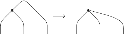
(Cerf theory for graphs) Any two cylindrical Cerf decompositions of a graph in a cylindrical bordisms are related by a finite sequence of critical point cancellations or creations, critical point/ vertex order reversals, vertex/critical point cancellations, and gluing elementary graphs with no critical points or vertices to adjacent elementary graphs.

We leave it to the reader to write out the exact definition of these moves which are analogous to those in Theorem 2.6. See Figures 9, 10, 11 for graphical representations of the moves.

Figure 9. Critical point/vertex switch

Figure 10. Vertex/vertex switch

Figure 11. Vertex/critical point cancellation

Proof.

The proof is similar to that of Theorem 2.6. Let $(f_{j},\underline{b}_{j})$ be two Morse data for $(Y,\Gamma,\phi)$ . We say that a homotopy $(f_{s})$ between $f_{0}$ and $f_{1}$ is good if except for a finite number of values of $s$ , each $f_{s}$ is a Morse function injective on its critical set and the critical set is disjoint from the vertices,

f_{s}|_{{\operatorname{Crit}}(f_{s})}:{\operatorname{Crit}}(f_{s})\hookrightarrow\mathbb{R},\quad{\operatorname{Crit}}(f_{s})\cap\operatorname{Vert}(\Gamma)=\emptyset

and at the remaining finite number of times $s_{1},\ldots s_{m}\in[0,1]$ at most one of the following occur:

(a)

critical point cancellation occurs in the interior of an edge:

$\exists y\in e,\quad{\mbox{d}}^{3}_{y}f_{s}|_{e}=0.$
(b)

a critical point occurs at an endpoint of an edge:

$\exists y\in\partial e,\quad{\mbox{d}}^{2}_{y}f_{s}|_{e}=0$

(c)

two critical points or endpoints have the same value:

\exists y_{1},y_{2}\in{\operatorname{Crit}}(f_{s}|_{\Gamma})\cup\operatorname{Vert}(\Gamma),\quad y_{1}\neq y_{2},\quad f_{s}(y_{1})=f_{s}(y_{2}).

Indeed, for no critical point cancellation to occur at the endpoints it suffices that for each endpoint $p$ and time $s$ , either ${\mbox{d}}f_{s}|_{e}(p)$ or ${\mbox{d}}^{2}f_{s}|_{e}(p)$ is non-zero. This is always the case for generic homotopies, since these conditions are codimension two. A small generic perturbation $f:Y\times[0,1]\to\mathbb{R}$ of the linear interpolation $sf_{0}+(1-s)f_{1}$ is a good homotopy, and furthermore has the cylindrical property

\partial_{t}f(y,s)>0,\forall(y,s)\in Y\times[0,1].

Breaking up the interval $[0,1]$ into subintervals each containing at most one critical time proves the theorem in a way similar to that of Theorem 2.6. ∎

The next step in the construction is to define a notion of admissible labellings of graphs. As in the case of tangles, this notion is designed to avoid reducibles in the moduli spaces of flat bundles.

Definition 5.10.

(a)

(Labels meeting a vertex) Let $(Y,\Gamma,\phi)$ be an elementary graph with a single vertex $v$ . Denote the boundary of $Y$ by $\partial Y=X_{-}\cup X_{+}$ . Let $B(v)\subset Y$ be a small open ball containing $v$ , and

$S(v)=\partial B(v),\quad\underline{x}(v):=S(v)\cap\Gamma$

denote the sphere around the vertex and the intersections with the graph. The complement $Y\kern-2.15277pt\smallsetminus\kern-2.15277ptB(v)$ of $B(v)$ can be viewed as a three-dimensional bordism from $X_{-}\cup S(v)$ to $X_{+}$ . It contains a tangle

$\Gamma\backslash(B(v)\cap\Gamma)\subset Y\kern-2.15277pt\smallsetminus\kern-2.15277ptB(v).$

Let $\underline{\mu}_{\pm}$ denote the labels for $\underline{x}_{\pm}=\Gamma\cap X_{\pm}$ , and $\underline{\mu}(v)$ denote the set of labels for $\underline{x}(v)$ , given by the labels of the edges incoming to a vertex and the images of the labels under the involution $*$ for the outgoing edges.
(b)

(Admissible labellings) A set of labels $\underline{\mu}(v)$ at a vertex $v$ is vertex-admissible if the moduli space of flat bundles on the punctured sphere is either empty or a point:

$\#M(S(v),\underline{x}(v),\underline{\mu}(v))\leq 1.$

An vertex-admissible labelling of $\Gamma$ is a labelling of the edges of $\Gamma$ by admissible labels, such that at each vertex the collection of labels is vertex-admissible. An vertex-admissible graph is a graph equipped with a vertex-admissible labelling.
(c)

(Standard labellings) Let $\omega_{j}$ denote the $j$ -th fundamental coweight of $SU(r)$ . Denote by ${\bf j}=\omega_{j}/2$ . Suppose that $G=SU(r+1)$ . A standard labelling of $\Gamma$ is a labelling of each edge by ${\bf 1}$ or ${\bf 2}$ , so that each vertex is trivalent with labels ${\bf 1},{\bf 1},*{\bf 2}$ , if all edges are incoming to the vertex.

The triple ${\bf 1},{\bf 1},{\bf 2}$ is analogous to Khovanov-Rozansky’s ${\bf 1},{\bf 2}$ (or thin, thick) labels [23].

Lemma 5.11.

Let $\underline{x}\subset S^{2}$ be a triple of distinct points. The moduli space $M(S^{2},\underline{x},{\bf 1},{\bf 1},*{\bf 2})$ is a point. Hence any standard labelling of a bordism-with-graph is admissible.

Proof.

The moduli space $M(S^{2},\underline{x},{\bf 1},{\bf 1},*{\bf 2})$ is the space of equivalence classes of pairs $(g_{1},g_{2})\in\mathcal{C}_{\bf 1}^{2}$ with $g_{1}g_{2}\in\mathcal{C}_{\bf 2}$ . After conjugation we may assume

g_{1}=\operatorname{diag}\left(-\exp(\pi i/r),\exp(\pi i/r),\ldots,\exp(\pi i/r)\right).

The centralizer of $g_{1}$ is therefore

Z=S(U(1)\times U(r-1))\cong U(r-1).

Let $O\subset G$ denote the one-parameter subgroup generated by rotation in the first two coordinates in $\mathbb{C}^{r}$ . Since $g_{1}$ is the product of $\operatorname{diag}(-1,1\ldots,1)$ with a central element in $U(r)$ , the adjoint action of $g_{1}$ on $O$ is $g_{1}og_{1}^{-1}=o^{-1}$ . This implies that

og_{1}=\operatorname{Ad}(o^{1/2})g_{1}\in\mathcal{C}_{1},\forall o\in O.

Now $\mathcal{C}_{\bf 1}$ is a symmetric space of rank one. The group $Z$ acts transitively on the unit sphere in $T_{g_{i}}\mathcal{C}_{\bf 1}$ . This implies that the map $Og_{1}\to\mathcal{C}_{\bf 1}/Z$ is surjective. Therefore after conjugation by an element of $Z$ we may assume that

g_{2}=og_{1}=g_{1}o^{-1}

for some $o\in O$ . Also note that since $O$ is conjugate to the one-parameter subgroup generated by the first coroot $\alpha_{1}^{\vee}$ the square of $\mathcal{C}_{1}$ in $G$ is

(24)

\mathcal{C}_{1}^{2}=\operatorname{Ad}(G)\{g_{1}^{2}o,o\in O\}=\bigcup_{\epsilon\in[0,-{1/2}]}\mathcal{C}_{\omega_{1}+\epsilon\alpha_{1}^{\vee}}

the union of conjugacy classes of $\exp(\omega_{1}+\epsilon\alpha_{1})$ where $\epsilon\in[0,-{1/2}]$ . In particular, since $\omega_{2}/2=\omega_{1}-\alpha_{1}$ the conjugacy class $\mathcal{C}_{2}$ of $\exp(\omega_{2}/2)$ appears in $\mathcal{C}^{2}_{1}$ . Hence the moduli space $M(S^{2},\underline{x},{\bf 1},{\bf 1},*{\bf 2})$ is non-empty, and a dimension count shows that it is dimension zero. Since the moduli space $M(S^{2},\underline{x},{\bf 1},{\bf 1},*{\bf 2})$ is connected, it consists of a single point. ∎

Lemma 5.12.

(Correspondence for vertex-admissible graphs is simply-connected and relatively spin) Let $\Gamma$ be an elementary graph containing a single vertex with incoming labels ${\bf 1},{\bf 1}$ and outgoing label ${\bf 2}$ . Then $L(Y,\Gamma,\phi)$ embeds in $M(X_{-},\underline{x}_{-})$ with spin normal bundle and fibers over $M(X_{+},\underline{x}_{+})$ with fiber $S^{2}$ . In particular $L(Y,\Gamma,\phi)$ admits a relative spin structure with background class $(b_{\pm}(X_{-},\underline{x}_{-}),b_{\mp}(X_{+},\underline{x}_{+}))$ for either choice of sign.

Proof.

Let $Y,\Gamma$ be as in the statement of the Lemma. By Lemma 5.11 the correspondence $L(Y,\Gamma,\phi)$ may be identified with the set of points in the moduli space for the incoming surface

[a_{1},\ldots,a_{2g},b_{1},\ldots,b_{h}]\in(G^{2g}\times\mathcal{C}_{\underline{\mu}_{-}-\{\bf 1,\bf 1\}}\times\mathcal{C}_{\bf 1}\times\mathcal{C}_{\bf 1})/\kern-3.01385pt/G,\quad b_{h-1}b_{h}\in\mathcal{C}_{\bf 2}.

It follows that the map $L(Y,\Gamma,\phi)$ to $M(X_{-},\underline{x}_{-})$ is an embedding and the map to the moduli space for the outgoing surface

M(X_{+},\underline{x}_{+})=(G^{2g}\times\mathcal{C}_{\underline{\mu}_{-}-\{\bf 1,\bf 1\}}\times\mathcal{C}_{\bf 2})/\kern-3.01385pt/G

has fiber equal to the quotient of stabilizers

(25)

S(U(2)\times U(r-2))/(S(U(1)\times U(r-1))\cap\operatorname{Ad}(\sigma_{12})S(U(1)\times U(r-1))\\ \cong S(U(2)\times U(r-2))/(S(U(1)\times U(1)\times U(r-2))\cong S^{2}

where $\sigma_{12}$ is the $(12)$ permutation matrix. The normal bundle for the embedding is determined by the image of the differential at the moment map at the level set $g_{1}g_{2}=\omega(\omega_{2}/2)$ . Since the stabilizer of $(\exp(\omega_{1}/2),\exp(s_{12}\omega_{1}/2))\in\mathcal{C}_{1}^{2}$ is $S(U(1)^{2}\times U(r-2))$ the normal bundle is the associated bundle

(26)

SU(r)\times_{S(U(2)\times U(r-2))}\left(\mathfrak{s}(\mathfrak{u}(2)\times\mathfrak{u}(r-2))/\mathfrak{s}(\mathfrak{u}(1)^{2}\times\mathfrak{u}(r-2))\right)\\ \cong SU(r)\times_{S(U(2)\times U(r-2))}\mathfrak{su}(2)/\mathfrak{u}(1)

which is spin.

Relative spin structures with the given background classes exist by the following argument. In the case of $(b_{-}(X_{-},\underline{x}_{-}),b_{+}(X_{+},\underline{x}_{+}))$ resp. $(b_{+}(X_{-},\underline{x}_{-}),b_{-}(X_{+},\underline{x}_{+}))$ a bundle with the given background class is obtained from descent of $T\mathcal{C}_{\bf 2}$ resp. $T\mathcal{C}_{\bf 1}^{2}$ to $M(X_{+},\underline{x}_{+})$ resp. $M(X_{-},\underline{x}_{-})$ , since tangent bundle to the fiber resp. the normal bundle is spin. ∎

Definition 5.13.

(Correspondence for vertex-admissible labellings) Suppose $(Y,\Gamma)$ is a graph with labelling $\underline{\nu}$ that is vertex-admissible for each vertex. Let $M(Y,\Gamma)$ denote the moduli space of flat bundles on the complement of $\Gamma$ in $Y$ with holonomies around the edges of $\Gamma$ given by $\underline{\nu}$ . Restriction to the boundary and pullback under the boundary identification define a map

(27)

M(Y,\Gamma)\to M(X_{-},\underline{x}_{-})^{-}\times M(X_{+},\underline{x}_{+}).

Denote the image of (27) by $L(Y,\Gamma,\phi)$ .

Lemma 5.14.

Let $(Y,\Gamma,\phi)$ be an elementary graph containing a single vertex and $\nu$ an admissible labelling of the edges of $\Gamma$ . Then $L(Y,\Gamma,\phi)$ is a smooth Lagrangian correspondence from $M(X_{-},\underline{x}_{-})$ to $M(X_{+},\underline{x}_{+}).$

Proof.

We write $\underline{\mu}_{\pm}\kern-2.15277pt\smallsetminus\kern-2.15277pt\underline{\mu}(v)$ resp. $\underline{\mu}_{\pm}\cap\underline{\mu}(v)$ for the labels of those markings in $\underline{x}_{\pm}$ that are not resp. are connected to $v$ by an edge. By (12), the symplectic forms on the two ends are those obtained by reduction from

(28)

\omega_{g,\underline{\mu}_{\pm}-\underline{\mu}(v)}+\omega_{0,\underline{\mu}_{\pm}\cap\underline{\mu}(v)}+(1/2)\langle\Phi_{g,\underline{\mu}_{\pm}-\underline{\mu}(v)}^{*}\theta\wedge\Phi_{0,\underline{\mu}_{\pm}\cap\underline{\mu}(v)}^{*}\overline{\theta}\rangle.

Let $d$ be the value of $f$ at the vertex and $\epsilon$ a small number. Choose a presentation for the fundamental group of $f^{-1}(d-\epsilon)$ ; then a presentation for the fundamental group of $f^{-1}(d+\epsilon)$ is obtained by replacing the generators for the strands incoming to the vertex with those outgoing. With respect to this set of generators, the correspondence defined by the bordism is given by

(29)

\prod_{\mu\in\underline{\mu}_{-}\cap\underline{\mu}(v)}c_{\mu}=\prod_{\mu\in\underline{\mu}_{+}\cap\underline{\mu}(v)}c_{\mu}

and descending to the quotient. The equation (29) defines an isotropic submanifold of $\mathcal{C}_{\underline{\mu}_{-}\cap\underline{\mu}(v)}^{-}\times\mathcal{C}_{\underline{\mu}_{+}\cap\underline{\mu}(v)}$ since the moduli space for the sphere around the vertex is a point by Lemma 5.11. It follows from (28) that the (29) defines an isotropic, hence Lagrangian submanifold of the product $M(X_{-},\underline{x}_{-})^{-}\times M(X_{+},\underline{x}_{+})$ . ∎

The following associates a generalized Lagrangian correspondence to any graph with admissible labelling:

Definition 5.15.

(Generalized Lagrangian correspondence for a decorated graph) Let $(f,\underline{b})$ be a cylindrical Cerf decomposition of $\Gamma$ equipped with vertex-admissible, monotone labels $\underline{\nu}$ . Let

L(Y_{j},\Gamma_{j},\phi_{j})\subset M(X_{j-1},\underline{x}_{j-1})^{-}\times M(X_{j},\underline{x}_{j})

denote the Lagrangian submanifold of representations that extend over $(Y_{j},\Gamma_{j})$ . Define

\underline{L}(Y,\Gamma,\phi):=(L(Y_{1},\Gamma_{1},\phi_{1}),\ldots,L(Y_{m},\Gamma_{m},\phi_{m})).

Proposition 5.16.

(Independence of the generalized Lagrangians from all choices up to equivalence) Let $(Y,\Gamma,\phi)$ be an admissible decorated graph from $(X_{-},\underline{x}_{-})$ to $(X_{+},\underline{x}_{+})$ . Then the generalized Lagrangian correspondence $\underline{L}(Y,\Gamma,\phi)$ is independent, up to equivalence, of the choice of Cerf decomposition.

Proof.

By Theorem 5.9 it suffices to check that the generalized Lagrangian correspondences are invariant up to composition equivalence under the Cerf moves. We check invariance in the case depicted in Figure 12 that two pieces $L(Y_{0},\Gamma_{0},\phi_{0})$ corresponding to an elementary graph with a single vertex, with strands say $j,j+1$ meeting at the vertex labelled ${\bf 1}$ and an outgoing strand labelled ${\bf 2}$ and $L(Y_{1},\Gamma_{1},\phi_{1})$ corresponding to a piece with a single critical point of index one connecting strands $j,j+1$ both labelled ${\bf 2}$ are replaced by a piece $L(Y_{01},\Gamma_{01},\phi_{01})$ with a single vertex with three strands $j-1,j,j+1$ , the last of which is outgoing but connected to the incoming surface. The correspondences may be identified with subsets of the incoming moduli spaces

L(Y_{0},\Gamma_{0},\phi_{0})\cong\{[a_{1},\ldots,a_{2g},b_{1},\ldots,b_{n}]\ |\ b_{j}b_{j+1}\in\mathcal{C}_{2}\}\subset M(X_{0},\underline{x}_{0})

L(Y_{1},\Gamma_{1},\phi_{1})\cong\{[a_{1},\ldots,a_{2g},b_{1},\ldots,b_{n-1}]\ |\ b_{j}=b_{j+1}\}\subset M(X_{1},\underline{x}_{1}).

Their composition is

L(Y_{0},\Gamma_{0},\phi_{0})\circ L(Y_{1},\Gamma_{1},\phi_{1})=\{[a_{1},\ldots,a_{2g},b_{1},\ldots,b_{n}]\ |\ b_{j}b_{j+1}=b_{j+2}\}.

Since the projection $L(Y_{0},\Gamma_{0},\phi_{0})\to M(X_{1},\underline{x}_{1})$ is a submersion, the composition is transverse. Hence

L(Y_{0},\Gamma_{0},\phi_{0})\circ L(Y_{1},\Gamma_{1},\phi_{1})=L(Y_{01},\Gamma_{01},\phi_{01})

as claimed. Invariance under the other moves is similar and left to the reader. ∎

Definition 5.17.

(Decorated Graphs) For coprime integers $r,d>0$ and a compact oriented surface $X$ let $\operatorname{Graph}(X,r,d)$ denote the category of graphs whose

•

objects are collections $\underline{x}$ of distinct oriented points of $X$ with admissible labels $\underline{\mu}$ ; that is, the same objects as for $\operatorname{Tan}(X,r,d)$ ;
•

morphisms are equivalence classes of labelled cylindrical graphs $(Y,\Gamma,\phi)$ ; and
•

composition of morphisms is given by gluing as in (1).

As before, the identity is the equivalence class of the trivial graph.

The following extends Theorem 3.22 to graphs.

Theorem 5.18.

(Symplectic-valued field theory for graphs) For coprime integers $r,d>0$ , the partially defined functor $\Phi:\operatorname{Graph}(X,r,d)\to\operatorname{Symp}_{1/2r}$ for elementary graphs extend to a field theory for graphs in $X$ .

Proof.

By Proposition 5.16, it suffices to show that the correspondences are equipped with relative spin structures; these are provided by Lemma 3.19 for correspondences involving critical points, and Lemma 5.12 for correspondences involving vertices. ∎

Using Corollary 4.9 we obtain a $A_{\infty}$ -category-valued field theory for graphs. In particular for any graph with admissible we obtain a functor between Fukaya categories

\Phi(\underline{L}(Y,\Gamma,\phi)):{\operatorname{Fuk}^{\begin{picture}(0.0,-10.0)\end{picture}}}(M(X_{-},\underline{x}_{-}),w)\to{\operatorname{Fuk}^{\begin{picture}(0.0,-10.0)\end{picture}}}(M(X_{+},\underline{x}_{+}),w)

which is independent of the choice of Cerf decomposition of the graph.

References

[1] S. Agnihotri and C. Woodward. Eigenvalues of products of unitary matrices and quantum Schubert calculus. Math. Res. Lett., 5(6):817–836, 1998.
[2] A. Alekseev, A. Malkin, and E. Meinrenken. Lie group valued moment maps. J. Differential Geom., 48(3):445–495, 1998.
[3] M. F. Atiyah and R. Bott. The Yang-Mills equations over Riemann surfaces. Phil. Trans. Roy. Soc. London Ser. A, 308:523–615, 1982.
[4] H. U. Boden and Y. Hu. Variations of moduli of parabolic bundles. Math. Ann., 301(3):539–559, 1995.
[5] A. Borel and J. De Siebenthal. Les sous-groupes fermés de rang maximum des groupes de Lie clos. Comment. Math. Helv., 23:200–221, 1949.
[6] S. Cautis and J. Kamnitzer. Knot homology via derived categories of coherent sheaves. II. $\mathfrak{sl}_{m}$ case. Invent. Math., 174(1):165–232, 2008.
[7] J. Cerf. La stratification naturelle des espaces de fonctions différentiables réelles et le théorème de la pseudo-isotopie. Inst. Hautes Études Sci. Publ. Math., (39):5–173, 1970.
[8] O. Collin and B. Steer. Instanton Floer homology for knots via $3$ -orbifolds. J. Differential Geom., 51(1):149–202, 1999.
[9] K. Fukaya. Floer homology for three manifolds with boundary I, 1997. Unpublished manuscript.
[10] K. Fukaya, Y.-G. Oh, H. Ohta, and K. Ono. Lagrangian intersection Floer theory: anomaly and obstruction., volume 46 of AMS/IP Studies in Advanced Mathematics. American Mathematical Society, Providence, RI, 2009.
[11] D. T. Gay and R. Kirby. Indefinite Morse 2-functions; broken fibrations and generalizations. arxiv:1102.0750.
[12] S. I. Gelfand and Y. I. Manin. Methods of homological algebra. Springer Monographs in Mathematics. Springer-Verlag, Berlin, second edition, 2003.
[13] W. M. Goldman. Invariant functions on Lie groups and Hamiltonian flows of surface group representations. Invent. Math., 85:263–302, 1986.
[14] M. Golubitsky and V. Guillemin. Stable mappings and their singularities. Springer-Verlag, New York, 1973. Graduate Texts in Mathematics, Vol. 14.
[15] V. Guillemin, V. Ginzburg, and Y. Karshon. Moment maps, bordisms, and Hamiltonian group actions, volume 98 of Mathematical Surveys and Monographs. American Mathematical Society, Providence, RI, 2002. Appendix J by Maxim Braverman.
[16] V. Guillemin and S. Sternberg. Birational equivalence in the symplectic category. Invent. Math., 97(3):485–522, 1989.
[17] R. Hartshorne. Residues and duality. Lecture notes of a seminar on the work of A. Grothendieck, given at Harvard 1963/64. With an appendix by P. Deligne. Lecture Notes in Mathematics, No. 20. Springer-Verlag, Berlin, 1966.
[18] Morris W. Hirsch. Differential topology, volume 33 of Graduate Texts in Mathematics. Springer-Verlag, New York, 1994. Corrected reprint of the 1976 original.
[19] M. Jacobsson and R. L. Rubinsztein. Symplectic topology of SU(2)-representation varieties and link homology, I: Symplectic braid action and the first Chern class. arxiv:0806.2902.
[20] V. G. Kac. Infinite-dimensional Lie algebras. Cambridge University Press, Cambridge, third edition, 1990.
[21] A. Keating. Dehn twists and free subgroups of symplectic mapping class groups. arxiv:1204.2851.
[22] M. Khovanov. Categorifications of the colored Jones polynomial. J. Knot Theory Ramifications, 14(1):111–130, 2005.
[23] M. Khovanov and L. Rozansky. Matrix factorizations and link homology. Fund. Math., 199(1):1–91, 2008.
[24] F. C. Kirwan. Cohomology of Quotients in Symplectic and Algebraic Geometry, volume 31 of Mathematical Notes. Princeton Univ. Press, Princeton, 1984.
[25] P. B. Kronheimer and T. S. Mrowka. Gauge theory for embedded surfaces. I. Topology, 32(4):773–826, 1993.
[26] P. B. Kronheimer and T. S. Mrowka. Knot homology groups from instantons. J. Topol., 4(4):835–918, 2011.
[27] D. Kwon and Y.-G. Oh. Structure of the image of (pseudo)-holomorphic discs with totally real boundary condition. Comm. Anal. Geom., 8(1):31–82, 2000. Appendix 1 by Jean-Pierre Rosay.
[28] L. Lazzarini. Existence of a somewhere injective pseudo-holomorphic disc. Geom. Funct. Anal., 10(4):829–862, 2000.
[29] J. Lurie. On the classification of topological field theories. In Current developments in mathematics, 2008, pages 129–280. Int. Press, Somerville, MA, 2009.
[30] C. Manolescu. Link homology theories from symplectic geometry. Adv. Math., 211(1):363–416, 2007.
[31] D. McDuff and D. Salamon. $J$ -holomorphic curves and symplectic topology, volume 52 of American Mathematical Society Colloquium Publications. American Mathematical Society, Providence, RI, 2004.
[32] V. B. Mehta and C. S. Seshadri. Moduli of vector bundles on curves with parabolic structure. Math. Ann., 248:205–239, 1980.
[33] E. Meinrenken and C. Woodward. Hamiltonian loop group actions and Verlinde factorization. Journal of Differential Geometry, 50:417–470, 1999.
[34] E. Meinrenken and C. Woodward. Canonical bundles for Hamiltonian loop group manifolds. Pacific J. Math., 198(2):477–487, 2001.
[35] J. Milnor. Lectures on the $h$ -cobordism theorem. Notes by L. Siebenmann and J. Sondow. Princeton University Press, Princeton, N.J., 1965.
[36] N. Nitsure. Cohomology of the moduli of parabolic vector bundles. Proc. Indian Acad. Sci. Math. Sci., 95(1):61–77, 1986.
[37] Y.-G. Oh. Floer cohomology of Lagrangian intersections and pseudo-holomorphic disks. I. Comm. Pure Appl. Math., 46(7):949–993, 1993.
[38] D. O. Orlov. Triangulated categories of singularities and D-branes in Landau-Ginzburg models. Tr. Mat. Inst. Steklova, 246(Algebr. Geom. Metody, Svyazi i Prilozh.):240–262, 2004.
[39] M. Poźniak. Floer homology, Novikov rings and clean intersections. In Northern California Symplectic Geometry Seminar, volume 196 of Amer. Math. Soc. Transl. Ser. 2, pages 119–181. Amer. Math. Soc., Providence, RI, 1999.
[40] A. Pressley and G. Segal. Loop groups. Oxford University Press, Oxford, 1988.
[41] P. Seidel. Lectures on four-dimensional Dehn twists. In Symplectic 4-manifolds and algebraic surfaces, volume 1938 of Lecture Notes in Math., pages 231–267. Springer, Berlin, 2008.
[42] P. Seidel and I. Smith. A link invariant from the symplectic geometry of nilpotent slices. Duke Math. J., 134(3):453–514, 2006.
[43] N. Sheridan. Homological mirror symmetry for Fano hypersurfaces. arXiv:1306.4143
[44] I. Smith. Floer cohomology and pencils of quadrics. Inventiones mathematicae 189: 149–250, 2012.
[45] E. Street. Recursive relations in the cohomology rings of moduli spaces of rank 2 parabolic bundles on the Riemann sphere. arxiv:1205.1730.
[46] M. Thaddeus. Geometric invariant theory and flips. J. Amer. Math. Soc., 9(3):691–723, 1996.
[47] M. Thaddeus. A perfect Morse function on the moduli space of flat connections. Topology, 39(4):773–787, 2000.
[48] K. Wehrheim and C. T. Woodward. Quilted Floer cohomology. Geom. Topol., 14(2):833–902, 2010.
[49] K. Wehrheim and C. T. Woodward. Floer cohomology and geometric composition of Lagrangian correspondences. Adv. Math., 230(1):177–228, 2012.
[50] K. Wehrheim and C. Woodward. Pseudoholomorphic quilts. To appear in Jour. Symp. Geom. arxiv:0905.1369.
[51] K. Wehrheim and C. T. Woodward. Functoriality for Lagrangian correspondences in Floer theory. Quantum Topol., 1(2):129–170, 2010.
[52] K. Wehrheim and C. Woodward. Exact triangle for fibered Dehn twists. To appear in Res. Math. Sci. arXiv:1503.07614.
[53] K. Wehrheim and C.T. Woodward. Floer field theory for coprime rank and degree. arXiv:1601.04924.
[54] K. Wehrheim and C.T. Woodward. Orientations for pseudoholomorphic quilts. arXiv:1503.07803.
[55] J. N. Mather. Stability of $C^{\infty}$ mappings. VI: The nice dimensions. In Proceedings of Liverpool Singularities-Symposium, I (1969/70), pages 207–253. Lecture Notes in Math., Vol. 192, Berlin, 1971. Springer.
[56] S. Ma’u, K. Wehrheim, and C.T. Woodward. ${A}_{\infty}$ -functors for Lagrangian correspondences. arXiv:1601.04919.
[57] E. Witten. Quantum field theory and the Jones polynomial. Comm. Math. Phys., 121(3):351–399, 1989.
[58] Edward Witten. Khovanov homology and gauge theory. In Proceedings of the Freedman Fest, volume 18 of Geom. Topol. Monogr., pages 291–308. Geom. Topol. Publ., Coventry, 2012.