Large Scale Power Suppression in a Multifield Landscape
Abstract
Power suppression of the cosmic microwave background on the largest observable scales could provide valuable clues about the particle physics underlying inflation. Here we consider the prospect of power suppression in the context of the multifield landscape. Based on the assumption that our observable universe emerges from a tunnelling event and that the relevant features originate purely from inflationary dynamics, we find that the power spectrum not only contains information on single-field dynamics, but also places strong constraints on all scalar fields present in the theory. We find that the simplest single-field models giving rise to power suppression do not generalise to multifield models in a straightforward way, as the resulting superhorizon evolution of the curvature perturbation tends to erase any power suppression present at horizon crossing. On the other hand, multifield effects do present a means of generating power suppression which to our knowledge has so far not been considered. We propose a mechanism to illustrate this, which we dub flume inflation.
1 Introduction
There is substantial evidence both on theoretical and observational fronts indicating that our observable universe underwent a period of inflation [1, 2, 3, 4]. If inflation really occurred, it provides an extraordinary opportunity to use observations of the Cosmic Microwave Background (CMB) and large scale structure as a means of studying particle physics at energy scales well above those likely to be achieved with terrestrial experiments. In particular, inflation is sensitive to Planck suppressed operators, allowing us to test ultraviolet complete theories in a unique way. It remains a central challenge for inflation to understand how it is to be embedded in such a theory but there has been significant progress in the context of string theory (for a recent review see [5]).
Developments in the understanding of compactification over the last decade have given rise to a striking picture that should have profound implications for the study of inflation — the prevalence of large Hodge numbers [6, 7, 8, 9] indicates the existence of many, often hundreds of scalar fields, interacting via a complicated potential containing a large number of metastable vacua. This picture is sometimes referred to as the string landscape [10, 11]. For inflationary phenomenology, arguably the most obvious consequences of this scenario are the possibility of multifield dynamics and the idea that our observable universe might have originated from a tunnelling event. Both of these behaviours present the alluring prospect of observable effects in the CMB.
The tunnelling process gives rise to an open universe inside the bubble of the new vacuum, whose initial evolution is dominated by spatial curvature [12]. This leaves an imprint on the power spectrum at scales crossing the horizon during this period [13, 14, 15, 16, 17] 11 1 Another possible observational consequence of this scenario is the detection of collisions between our bubble and other topological defects [18] or bubbles [19, 20, 21, 22] created in the parent vacuum. This is an interesting possibility that is currently being actively investigated.. If the inflationary epoch inside the bubble is short enough, one could hope to see this effect in the low- (largest observables scales) regime of the CMB spectrum. This possibility is heavily constrained by the latest Planck data [23], which sets a bound on the scale of curvature as being at least an order of magnitude bigger than the scale of today’s horizon, implying that the scales we observe left the horizon after curvature domination.
Multifield effects are potentially very important for inflation embedded in fundamental physics. Obtaining an extended period of inflation is notoriously difficult in string theory but it is often the case that whatever mechanism enables one field to be sufficiently light, will tend to make other fields sufficiently light to be cosmologically relevant as well. This point has been emphasised in a large body of work but the message in Ref. [24] is particularly succinct; multifield dynamics should be considered the norm in string theory.
Inflation with more than one light field can in principle give rise to a wide range of signatures, generally (but not exclusively) as a consequence of the superhorizon evolution of the primordial curvature perturbation, which in turn is a consequence of the presence of isocurvature degrees of freedom. Currently there is no observational evidence for any of these signatures, implying no evidence of multifield inflation. However it should be noted that this does not provide a confirmation against these scenarios either, since many models that exhibit multifield dynamics do not break the single-field predictions enough to be under threat from current constraints (see for instance [25, 26, 27, 28, 29, 30, 31, 32, 33]).
In this work we will focus on the particularly interesting observation of a possible suppression of the power spectrum on large scales, as suggested by the WMAP [34] and Planck [35] data. There has been considerable interest in studying mechanisms for this lack of power [36, 37, 38, 39, 40, 41, 42, 43, 44, 45, 46, 47, 48, 49, 50, 51, 52], in particular as a consequence of the inflationary era, but its possible microphysical origin remains undisclosed. It was pointed out in Ref. [53] that tunnelling from a metastable vacuum through a potential barrier might naturally generate a period of steep inflaton potential before the slow-roll plateau. Should we be fortunate enough that the total period of inflation is sufficiently small and, at the same time, long enough to avoid the constraints of curvature, we could hope to see the onset of this epoch imprinted in the CMB as some form of signature on large scales. Of key relevance to this paper, Bousso, Harlow and Senatore [45, 40] emphasised that in the case of a theory consisting of a single scalar field, power suppression is a likely consequence of this tunnelling in the landscape.
The possibility that power suppression may be a consequence of the string landscape is extremely exciting, as it would represent a unique door to the physics of the early universe. However there is a considerable way to go before such claims can be made. Building on the work of Ref. [45, 40], an obvious next question to ask in furthering this pursuit is does power suppression also occur if more than one field is involved in this event?
The tunnelling process in a multifield model can be quite complicated and one might expect the initial condition after the transition to be quite far from the inflationary plateau region that leads to most of the observable scales in the CMB, the range 22 2 See [54] for a proposal that links the position of the fields after the tunnelling event to the inflationary region in a multifield landscape.. One can expect scenarios where many moduli fields are affected by the tunnelling transition, potentially giving rise to a rich mass spectrum of the scalar fields involved in inflation. As an example of hierarchies in the mass spectrum, one can conceive that tunnelling would affect different moduli sectors in distinct ways. This could result, for example, in a situation where at first inflation is controlled by the evolution of complex structure moduli and then, as these fields settle into their minima, becomes dominated by a different moduli sector, like a Kähler moduli field. Many current models of compactification naturally lead to this kind of hierarchies in the mass spectrum and separation in scalar sectors, indicating that multifield dynamics are relevant after tunnelling events (see, for example Ref. [6]). In this paper we explore how the single-field results of power suppression on large scales generalise in the presence of many scalar fields with such rich mass hierarchies.
We start our discussion by reviewing a simple method to compute the power spectrum and the spectral index in a multifield inflationary context. We then review the mechanism of power suppression due to a steepening of a single-field potential as described in Ref. [45, 40], and look at the consequences of including more than one light field in this scenario. Our main result is that achieving power suppression is considerably more delicate in a multifield model than in the single-field case. In fact, a steep potential and a fast evolution during the first few e-folds of inflation do not necessarily imply suppression of the power spectrum on large scales. We identify strong constraints imposed on initial conditions as well as inflaton potential in the region resulting in suppression. These constraints apply not only to the form of the potential along the inflationary trajectory but to all other directions in field space. This is a rare opportunity where 2-point statistics can be used to learn about multifield effects.
If all relevant features originate purely from an inflationary era, suppression on large scales would then constrain multifield dynamics in a region where one also requires non-trivial evolution of the slow-roll parameter . We argue that the ability to learn about the mass spectrum at such a crucial stage of inflation has significant implications for model building in the context of the string landscape.
To conclude, we present a novel approach to obtain relative power suppression on large scales based entirely on superhorizon evolution of the perturbations. Here the idea is not to suppress the power at large scales but to enhance it at smaller scales by continuously transferring power from isocurvature to adiabatic modes. We present a simple example where this can happen which could be relevant for some string theory scenarios.
2 Multifield inflation — a geometrical picture
Our goal is to gain intuition about the phenomenology underlying power suppression and so to aid us in this task we will compare two methods of computing the perturbations. One approach is the transport method — a fully numerical approach which solves for the field–field, field–momenta and momenta–momenta correlation functions, which we do not review here. We use the publicly available Mathematica code available from transportmethod.com to perform our analyses and refer the reader to Ref. [55] for a detailed description of the method. Our second approach is a slow-roll superhorizon analysis of the perturbations which we do now review. The key benefit of this second method is that it enables one to derive a number of analytic or semi-analytic expressions which will be our primary tool in understanding the phenomenology underlying our numerical results.
Restricting our studies to superhorizon scales and assuming the slow-roll approximations radically simplifies the computation of observable quantities. On superhorizon scales the field perturbations evolve classically in the sense that decaying solutions to the mode equations have died away. The upshot of utilising the slow-roll equations is that the evolution of all quantities of interest can be understood purely in terms of gradient flow. Hence a problem which in principle requires understanding potentially complicated operator equations, under these restrictions, reduces to a question of computing relatively simple geometrical quantities in field space. This simplification has been used in a very large body of work and is intimately related to the celebrated separate universe assumption [56, 57, 58, 59, 60]. We refer the reader to Ref. [61] and references therein for a more detailed discussion. The notion of using geometrical quantities to compute observables was most heavily emphasised in [61, 62, 63, 64] and it is these works which we summarise here.
Throughout this paper we work in units of , so that the reduced Planck mass reads , and assume the background space-time metric to be the Friedman-Robertson-Walker with “mostly plus” signature
| (2.1) |
2.1 Background equations of motion
We will consider models describing the inflationary dynamics of a set of n real scalar fields, , . Restricting ourselves to theories involving at most two space-time derivatives, the action can be written as
| (2.2) |
where is an arbitrary symmetric matrix and is the scalar potential. The matrix is usually interpreted as a metric on a dimensional scalar manifold parametrized by the fields . The equations of motion for the homogeneous background fields are
| (2.3) |
where dots denote derivatives with respect to cosmological time, is the Hubble parameter, and we have defined the covariant derivative involving the Christoffel symbols associated to as .
In the following we will focus on the evolution of the set of fields that are light enough to be part of the slow-roll dynamics. This does not preclude the existence of a heavy sector but we will assume that these other fields do not play a significant role for the background or the perturbations. However, situations where this assumption fails can be captured using the transport method and we do include examples of this in later sections.
The slow-roll conditions in the multifield case can be defined in terms of the parameters 33 3 We raise and lower indices using the metric and its inverse .
| (2.4) |
Under these conditions, the equations of motion reduce to gradient flow equations
| (2.5) |
where we have used the short hand notation to refer to derivatives with respect to the number of e-folds .
2.2 Evolution of scalar perturbations
To study fluctuations about the homogenous background we choose to work in the flat gauge such that the independent degrees of freedom are the fluctuations in the fields . These perturbations transform covariantly under a change of coordinate basis. In other words, should be interpreted as a tangent vector rather than a coordinate displacement [65]. Our task now is to derive an equation of motion for these perturbations. There are at least two ways to do this. One method is to perturb the action (2.2) as was done in Refs. [66, 58, 55], however, given our simplifying assumptions of only considering superhorizon scales in the slow-roll regime, there is a more direct method which is to instead perturb Eq. (2.5). The separate universe assumption provides an intuitive picture of why this method works. It states that when spatial patches are smoothed on a scale much larger than the horizon scale, the average evolution of each patch evolves according to the background equations of motion [56, 57, 58, 59, 60]. The resulting picture in field space is a bundle of non-interacting trajectories, each evolving according to Eq. (2.3) but subject to perturbed initial conditions. When slow-roll holds such that Eq. (2.5) applies, this description becomes precisely analogous to geometrical optics [61]. Hence, the field fluctuations may be interpreted as Jacobi fields satisfying [66, 62, 64, 61]
| (2.6) |
where can be seen as an effective mass matrix, which encodes the couplings between the fields as well as a correction due to the non-trivial geometry of the scalar manifold. Denoting to be the components of the Riemann tensor on , the matrix is defined as 44 4 In the slow-roll limit we must also require that
| (2.7) |
Ultimately the principal observables of interest are the correlation functions of the primordial curvature perturbation . We therefore need an expression that relates field perturbations in the flat gauge to the primordial curvature perturbation in the constant density gauge 55 5 We choose to work with , the curvature perturbation in the constant density gauge, but we could have equally worked in the comoving gauge where the curvature perturbation is usually denoted . Both of these quantities can be computed using cosmological perturbation theory and are known to be equal at second order on superhorizon scales up to corrections [67, 68].. This gauge transformation can be computed using cosmological perturbation theory, however once again the separate universe assumption enables us to take a shortcut. Lyth and Rodríguez [60] showed that the separate universe assumption can be used as a practical means of computing since on superhorizon scales , the variation in the number of e-folds between an initial flat slice and a subsequent constant density slice. At lowest order we have
| (2.8) |
where and for clarity in discussions to follow, we have explicitly labeled the fact that all quantities are to be evaluated at the final time of interest . We refer the reader to Ref. [69] for a recent discussion of this topic and detailed derivations of this expression as well as higher order expressions using both cosmological perturbation theory and the separate universe assumption.
So far we have implicitly been working on the coordinate basis for our perturbations, meaning the basis vectors are aligned with the original fields. One can also look at the vector of perturbations projected onto the so-called kinematic basis [70, 71, 62, 64] defined by a set of n orthonormal vectors satisfying
| (2.9) |
where , and we have denoted the dot product between vectors by . Note that the quantity , which by definition we choose to be non-negative, only vanishes when the background follows a geodesic trajectory, i.e. when . The advantage of this basis is that by comparison with Eq. (2.8), one can immediately identify the projection of the field perturbations along the inflationary trajectory with the primordial curvature perturbation . One can then write the following decomposition of the perturbations in the kinematic basis corresponding to the time
| (2.10) |
In this basis, the equations of motion for the superhorizon evolution of the perturbations become, 66 6 Note that after switching to the the orthonormal basis (2.9) there is no distinction between upper and lower indices. See Appendix A for a more detailed explanation of these expressions.
| (2.11) |
where refers to the element , not to be confused with an exponent 2. We have introduced the matrix
| (2.12) |
that describes how quickly the kinematic basis vectors change along the inflationary trajectory; in other words, it expresses the turn rates of the basis vectors.
Looking at the equations of motion for the perturbations in this decomposition one can easily see two very important points. The first equation tells us that the curvature perturbation is not constant, as it can get sourced by isocurvature modes via the first mode . This will happen whenever there are turns in the trajectory in field space, or in other words, deviations from a geodesic motion, as this makes non zero. The rest of the equations provide information about the evolution of isocurvature modes, which are controlled by the masses of the fields as well as possible turns of the inflationary trajectory.
The solution to the set of equations (2.6) or (2.11) can be formally expressed without any loss of generality in terms of a transfer matrix which describes the evolution from time at horizon exit to a subsequent time
| (2.13) |
where the subscript () represents evaluation at horizon exit. Thus, all the information about the superhorizon evolution of the perturbations is encoded in the transfer matrix . Using the decomposition Eq. (2.10), the transfer matrix takes a particularly simple form. Setting
where the block has the same dimensions as a vector and is an matrix which represents the evolution of the entropy mode vector from horizon exit to the end of inflation. The matrix entry represents the requirement that curvature perturbations are conserved on superhorizon scales in the absence of entropy modes and that curvature perturbations do not source entropy modes after horizon crossing [72].
In using the “” approach to computing , so far we have been taking the flat surface and constant density surface to be infinitesimally separated. A useful alternative is to take the flat surface to be at horizon crossing
| (2.20) |
Written this way, all details of the superhorizon evolution are contained in the vector . By direct comparison with Eq. (2.2) we can find and expression for in terms of the components of the transfer matrix 77 7 Despite the fact that the vector contains information about the full superhorizon evolution, it belongs to the tangent space of at the point , and therefore it is decomposed in the kinematic basis corresponding to the time of horizon crossing . This is to be contrasted with Eq. (2.10), where the kinematic basis is that of . This implies a slight abuse of notation since we express the kinematic basis associated to these two different times with the same symbols .
| (2.21) |
We call the angle between and the direction of gradient flow at horizon crossing the correlation angle . Since and are orthogonal to each other, using Eq. (2.21) we conclude that
| (2.22) |
where , is the unit vector in the direction of , and the correlation angle is defined such that . This quantity, as will become clear shortly, is a very convenient measure of the superhorizon evolution of .
2.3 Two-point statistics
We define the power spectrum of the curvature perturbation to be
| (2.23) |
To make use of expression (2.20), we need to specify the conditions for the perturbations at horizon crossing. Provided the inflationary trajectory is not turning too much and slow-roll approximations hold so that is approximately constant, it is reasonable to assume all perturbations to be decoupled. Under these assumptions, the 2-point function for the field perturbations in a local frame where the fields have canonical kinetic terms, can be expressed as
| (2.24) |
where a star () indicates evaluation at the comoving scale .
Applying the transfer matrix to the spectra at horizon crossing one immediately finds that the spectrum of curvature perturbations at the end of inflation has the form [73, 70, 62, 71]
| (2.25) |
Since at horizon crossing , according to Eq. (2.8), we see this expression can be simply written in terms of the correlation angle as
| (2.26) |
Provided perturbations are small, this result relies solely on the assumption that the spectrum of perturbations is well described by Eq. (2.24) at horizon crossing. Note that an important consequence of assuming the field perturbations to be uncorrelated at horizon crossing is that to leading order in the the slow-roll parameters, superhorizon evolution of the scalar perturbations always gives a positive semidefinite contribution to the power spectrum.
As we mentioned earlier, we can see from Eq. (2.11) that for we need sizeable entropy perturbations, i.e. isocurvature should not decay too fast, and we should also have mode mixing, that is, the effective mass matrix should have non-zero off diagonal terms. In the slow-roll regime the presence of mode mixing occurs whenever the inflationary trajectory deviates from the geodesic motion, or in other words, when it describes a turn in field space. In Eq. (2.11) these effects are encoded in the matrices and . As we shall see in later sections these remarks have important consequences when trying to implement large scale suppression of the power spectrum in multifield inflationary models.
We conclude this section by presenting an expression for the spectral index in this geometrical framework. As shown in Appendix B, in the slow-roll regime the spectral index can be written in a very compact way as
| (2.27) |
This expression is the same as that found in Ref.[58], which is the generalisation of the one presented in Ref. [62] for two-field inflation in the slow-roll slow-turn regime. Note that this result implies that the spectral tilt is determined by two local quantities, and , and one non-local quantity, the unit vector which depends on the details of the whole inflationary trajectory between the time of horizon-crossing and the end of inflation , since it depends on the transfer function . When there is no superhorizon evolution the transfer matrix (2.2) reduces to the identity matrix, implying that and is parallel to the direction of the inflationary trajectory . However, in general can point in any arbitrary direction with determining the relative angle between and .
3 Power suppression in single-field inflation
To understand the idea behind power suppression in the presence of a steepening of the potential, let us briefly discuss the case of single-field models. In this case, assuming slow-roll is a good approximation at horizon crossing, the power spectrum for the scale that crosses the horizon at is given by
| (3.1) |
Since during inflation the Hubble parameter is approximately constant, to realise , with , requires that . In other words, power suppression between and can only occur if the slow-roll parameter is decreasing between the times of horizon exit of these scales, and respectively. This implies that the potential should be steeper between and than in the subsequent inflationary evolution.
The simple example proposed in Refs. [45, 40] illustrates this idea well. The potential has the general form
| (3.2) |
where is the “slow” part of the potential, modelled as a Taylor expansion with coefficients chosen to match observational constraints
| (3.3) |
The mass scale is fixed by cobe normalisation [74] and makes and (and in particular ) dimensionless. The early stages of inflation are dominated by a brief period of “rapid” evolution on a steeper potential , that should be steep enough to provide the desired power suppression. According to Refs. [45, 40], these requirements are satisfied by a quadratic potential like
| (3.4) |
where can be chosen to produce power suppression at , as we do for example in the right plot of Fig. 1.
The key observation made in Ref. [40] is that for the model given by Eq. (3.2) one can obtain an approximate expression for this power spectrum, when , of the form
| (3.5) |
where is the power spectrum that would be obtained by considering only. Importantly this expression shows that the effect of is always to suppress the power spectrum. This is intuitive, as provided Eq. (3.1) holds, one sees that the effect of the “rapid” phase manifests as increasing the magnitude of .
To understand more accurately the power suppression induced by the presence of , one should take into account the deviations from the slow-roll approximation or from (2.24) induced by the period of rapid evolution. For this we performed a full numerical evolution of the background and two-point correlation functions of the fluctuations (which does not rely on slow-roll approximations) [55] 88 8 Our numerical approach is the non-slow-roll version of the Transport method. We refer the reader to Refs. [55, 75, 76, 61, 77] for more information on this approach.. For simplicity, and consistency with Refs. [45, 40], curvature effects were completely ignored in the evolution equations. We believe that given the current constraints on spatial curvature this approximation should not impact on our main results, which refer to scales leaving the horizon after the curvature bound has been reached. In addition, if our observable universe tunnelled from a parent metastable vacuum, and inflation started earlier than the horizon-crossing time for the largest observable scale in order to dilute curvature artefacts, it seems reasonable to assume a Bunch–Davies state as our initial conditions at this time. This is the starting point of our numerical evolution which we define to be at 99 9 The initial state after tunnelling is known to be affected by the parent vacuum as well as other effects associated to the nucleation process. Our assumption is that these effects are small for the cases studied in this paper. This point has recently been investigated in [49]. Their conclusions indicate that this would be a small effect.. The results of the simulations are displayed in Figs. 1 and 2.
In Fig. 1 we have displayed how the power spectrum varies for different choices of the mass parameter which determines the steepening, while the other two parameters in the potential, and , are kept fixed for simplicity. The spectrum in these plots interpolate between the spectrum of quadratic inflation for large scales and the one of linear inflation for small scales. The transition point corresponds roughly to the point where the spectral tilt changes abruptly from positive to negative. The figure shows that, as the “rapid” region of the potential becomes steeper (for increasing values of ), the power suppression in the 4 e-folds prior to the transition becomes more pronounced, and at the same time the range of scales which experience power suppression decreases.
In order to identify which models are capable of producing power suppression on large scales, it is useful to observe that the suppressed spectra necessarily have a positive (blue) tilt i.e. , at some point during the first e-folds of the observable inflation. We therefore use the deviations of the spectral index on large scales as a marker for the existence of power suppression. As we discussed in the previous section, the general expression for the spectral index in the multifield case is complicated by the fact that it involves non-local terms. However, in the case of single-field inflation, things become much simpler since the vector necessarily coincides with the direction of the inflaton , and therefore the expression for the spectral index to leading order in the slow-roll parameters, Eq. (2.27), reduces to the usual formula
| (3.6) |
Here is the second slow-roll parameter of single-field inflation given by . Using this expression for the spectral index we can translate the blue tilt condition on the spectrum into a constraint on the inflationary potential. According to Eq. (3.6), a blue tilt for the scale occurs whenever
| (3.7) |
We expect the slow-roll approximation to be in good agreement with the numerical result for scales exiting the horizon well away from the transition between the rapid and slow parts of the potential. However scales leaving the horizon during the transition between these two periods of inflation can experience effects that cannot be captured by the slow-roll description. One effect is the mixing of mode functions, which gives rise to oscillations in as can be seen in Fig. 2. This effect is well studied and we refer the reader to Refs. [36, 47, 48] for more detailed discussion 1010 10 Recently, in Ref. [48], a study of the implications of different equations of state at the beginning of inflation was performed (for related work see [78, 79]). In this paper [48], authors considered an instantaneous change between pre- and inflationary eras. We believe that slow approaches to the inflationary attractor might also have interesting phenomenological consequences..
In the left plot of Fig. 2 we compare the numerically obtained non-slow-roll result with the slow-roll approximation which we obtained solving the gradient flow equation Eq. (2.5) and assuming slow-roll at horizon crossing, Eq. (3.1). When the mass is small, as for the model parameters discussed in Refs. [45, 40], then the non-slow-roll correction is small. However, it is noteworthy that increasing the mass does not simply reduce the range of scales over which power suppression occurs; we also see that the oscillations became large. An example of this is shown on the right plot of Fig. 2, where we compare the spectra obtained with and . If the potential is too steep the resulting power spectrum could be ruled out by observations, imposing important constraints on this model as a viable method to obtain power suppression.
4 Power suppression in multifield inflation
The construction of multifield inflationary models which display suppression of the power spectrum at large scales is more subtle than in single-field models. Consider the ratio of the power spectrum at two different scales which exit the horizon at the times and respectively. In order for the power spectrum to be suppressed at the scale with respect to we need to have
| (4.1) |
In other words, this ratio depends on the relative amount of superhorizon evolution experienced by scales and , which in turn depends on the relative size of the corresponding correlation angles . Recall that is the angle between the gradient of the number of e-folds, parallel to , and the inflaton direction at the time , . For a given ratio at horizon exit, we can find two different situations:
- •
: When the correlation angle is smaller for the smaller scale the superhorizon evolution acts as to reduce the power suppression existing at horizon exit
(4.2) As a consequence of this, to have power suppression at the end of inflation in this scenario, it is not sufficient to have it present at horizon crossing.
- •
: When the correlation angle is smaller for the larger scale the superhorizon evolution acts as to enhance the power suppression existing at horizon exit
(4.3) In this situation power suppression might be present at the end of inflation even when it is absent at horizon crossing, i.e. .
For an inflationary model to be predictive, inflation must reach the adiabatic limit before the end of inflation. In scenarios where this is the case, it seems reasonable to expect that scales exiting the horizon at later times experience progressively less superhorizon evolution. From this perspective, the first situation seems somehow more typical than the second one. The second situation can occur, for example, when a very massive field suddenly becomes light at some point between and . In that case, low power at large scales arises because of a power enhancement at small scales. In the next section we will show a concrete example of the first situation, and in § 6 we will present an example of the second.
Analysis of the spectral index:
Similarly to the case of single-field inflation, a useful way to translate the conditions for power suppression into constraints on the form of the potential is to look at the evolution of the spectral index. As we argued above, the presence of suppression at large scales requires a period where the tilt transitions to blue. In the multifield case a blue tilt for the scale occurs whenever
| (4.4) |
in other words, whenever the projection of the effective mass matrix along the vector is larger than the slow-roll parameter . In general the vector will not point in the direction of the inflationary trajectory and therefore, in contrast to the single-field case, the condition above is unrelated to the steepness of the potential. In fact, the steepening of the potential is neither necessary nor sufficient to guarantee a period of blue tilt in the large scale power spectrum.
To understand the constraints on the potential around the inflationary trajectory, it is convenient to express Eq. (4.4) in terms of the Hessian of the scalar potential, rather than which is related to the Hessian of :
| (4.5) |
When the field space metric is flat everywhere the curvature term in the definition of is absent and it reduces to the Hessian of . Since the diagonal elements of any hermitian matrix are always bounded above by the largest eigenvalue, this condition implies that the largest eigenvalue of must be larger than at least . Therefore, a necessary but not sufficient condition to have a blue tilt in the spectrum at a given scale is that the largest mass of the system evaluated at horizon exit satisfies
| (4.6) |
In the same way, since diagonal elements of a hermitian matrix are bounded below by the minimum eigenvalue, we find the sufficient but not necessary condition for blue tilt at
| (4.7) |
In other words, when this condition is satisfied the power spectrum will always be blue-tilted at , irrespective of the superhorizon evolution experienced by the mode after horizon exit.
5 Example I: plateau preceded by quadratic inflation
In this example we consider the situation where . We discuss a two-field model where the fields have canonical kinetic terms , and we define the scalar potential to be
| (5.1) |
Here and remain the same as in Eqs. (3.3) and (3.4), and is given by
| (5.2) |
This illustrates the picture where a mass hierarchy is present in the scalar sector resulting in non-trivial dynamics before the inflationary plateau. This is the typical situation after a tunnelling event where the initial conditions for inflation are generically far away from the inflationary region of the potential.
The first thing we can tell about this model is that in order to have power suppression, according to the necessary condition (4.6), we require that during some period
| (5.3) |
where we have also used that in the steep region of the potential and . If this condition is not satisfied, no slow-roll inflationary evolution will lead to a blue-tilted power spectrum, and therefore we can not have power suppression on large scales.
Conveniently, this potential belongs to the sum-separable class
| (5.4) |
for which it is possible to calculate analytic expressions for observable quantities, provided the background evolution is well approximated by the slow-roll equations and the kinetic terms are canonical. Specifically, the vector in these models can be written as [80]
| (5.5) |
where are a set of functions that become constant in the adiabatic limit. Without loss of generality we can always rearrange the constant terms of the summation such that 1111 11 If a field reaches the minimum of its own potential during inflation , it is always possible to redefine the potential such that also vanishes at that point. It can be shown that this choice implies that the corresponding has to be zero at (see [80, 81]). . Thus, using Eq. (2.25), we have that
| (5.6) |
which depends exclusively on quantities evaluated at horizon crossing, even though it encodes all superhorizon evolution of the power spectrum. The term in curly brackets can be thought of as the result of transferring power from isocurvature perturbations to adiabatic perturbations on superhorizon scales. Using this expression and the condition for power suppression Eq. (4.1), we can immediately find constraints on the potential. The requirement for power suppression is not a period of inflation with relatively larger (like in single-field inflation), but a period where the summation is smaller1212 12 the explicit factor in Eq. (5.6) cancels with the term in the denominator of ., which is a significantly more intricate condition.
To better understand how this translates to constraints on initial conditions it is convenient to express Eq.(5.6) in terms of the correlation angle. Remembering that is the angle between and
| (5.7) |
and that , we obtain
| (5.8) |
When the system is in its adiabatic limit the two directions coincide and . Conversely, for large values of the correlation angle is close to , implying that in this regime the perturbations will experience a large amount of superhorizon evolution. Using the previous result it is straightforward to derive an upper bound for the magnitude of power suppression in the multifield case
| (5.9) |
For an analysis of initial conditions, it is convenient to make a change of variables in field space such that
| (5.10) |
and start the trajectories always at the same height, from a fixed value of the scalar potential . These initial conditions define a curve in field space which is characterised by a function . Expressing and in terms of and , and keeping only the leading order terms in the slow-roll parameter , we can rewrite Eq. (5.9) as
| (5.11) |
where is the initial height above the inflationary plateau. As we require our model to approach the adiabatic limit in order to be predictive, for simplicity we will assume that this limit is reached shortly after the steep region of the potential, such that . Moreover, we will also suppose that at this point the inflaton is rolling down the inflationary plateau where . In this case, the condition for power suppression can be expressed in terms of a maximum value of the initial angular direction, , above which power suppression cannot be realised:
| (5.12) |
Scenario One
The effects of isocurvature are especially evident in the case . As argued in § 4, in order to have power suppression at horizon crossing the inflationary trajectory needs to experience a steepening, and in this case the rapid evolution occurs in a different field direction to the slow phase, i.e. along . This naïvely looks like a small change from the single-field scenario since one can still arrange for the trajectory to follow very similar values of the potential thus resulting in a similar profile for . However the role of multifield effects turns out to be very important – when the superhorizon evolution is taken into account the power suppression disappears, completely. This follows directly from Eq. (5.12), as the critical angle vanishes and therefore there are no initial conditions for which one can realise power suppression.

The evolution of the power spectrum on each scale from horizon exit up to the end of inflation is shown in Fig. 4. Around horizon crossing, one sees significant power suppression on large scales (for ) but soon after these scales leave the horizon, the field-space trajectory goes through a turn (see Fig. 3), causing the isocurvature perturbation to source the adiabatic perturbation and hence evolves in such a way as to erase any information about the steepening of the potential that was there initially.
The change in the spectral tilt displayed in the right plot of Fig. 4 can be understood easily from the multifield expression of the spectral index Eq. (2.27). Consider a trajectory starting at some large value of — initially points roughly along the direction and points along the direction (see Fig. (3)). If there was no superhorizon evolution, the spectral index would then reduce to
| (5.13) |
implying that at a certain height of the potential we could have a blue-tilted spectrum by choosing to be sufficiently large. This would be the naïve conclusion one would get by studying the spectrum at horizon crossing. However, making superhorizon evolution into account, from the bound (5.8), we see that at large the correlation angle should be close to , implying that points instead along the direction of . As a consequence, using Eq. (2.27) with , we find that the spectral index is smaller than one
| (5.14) |
i.e. the spectrum is red-tilted at the end of inflation. This comparison is shown explicitly in the right plot of Fig. 4.
Scenario Two
In our second scenario we consider the effects of having a non-zero value for . Taking to be the same as in the left-hand plot of Fig. 1, i.e. appropriately chosen to manifest power suppression when the second field is placed at its minimum, we conclude that the results depend heavily on the choice of initial conditions. In Fig. 5 we show the inflationary trajectories and corresponding power spectra of the cases , and respectively. In these cases depending on the choice of initial conditions the result interpolates between the full suppression of the single-field model and no suppression, when plays a significant role in the evolution, as occurs in the previous example.
The left-hand plots show the slow-roll inflationary trajectories for each case. The red lines correspond to inflationary trajectories where the corresponding power spectrum displays suppression. For convention, we say that a power spectrum has suppression when the deficit of four folds before transition with respect to the transition itself
| (5.15) |
is at least half of what it is obtained in the single-field case. The plots illustrate that the angle increases with the magnitude of , as expected from the formula (5.12).
Scenario Three
For completeness, our third scenario is the same as the last one, except now . This case cannot be treated using the slow-roll approximations since displacement of the second field can give rise to significant oscillations. As expected from basic considerations of effective field theory, as the limit is approached, the situation becomes simpler and the broad features match that of the single-field result. The difference is that now we also see oscillations on the largest scales as a result of excitation of the second field; see Fig. 6. This last scenario displays essentially the heavy physics phenomenology that has been studied in, for example, Refs. [82, 83, 84, 85, 86, 87, 88] and references therein.
The nature of the oscillations of a second field are different to that of the mixing of modes observed in the single-field scenario. It was shown in Refs. [85, 84] that the features related to the decay of a heavy mode behave as
| (5.16) |
where is the mass of the heavy field and is the unperturbed power spectrum. The mixing of modes as a result of a sudden change in the background evolution [89, 36, 90] gives rise to a different oscillatory profile. Even though the amplitude of oscillations is sensitive to details of the period of rapid evolution, in the short wavelength limit it is possible to characterise their frequency and decay rate in a relatively model independent way.
Provided the density perturbations asymptote to the Bunch-Davis vacuum for scales deep inside the horizon, the power spectrum has the following characteristic behaviour for (see Ref. [89])
| (5.17) |
where is the value of the scale factor at the transition . With sufficiently high quality data one could hope to distinguish these two signatures.
6 Example II: Power suppression from superhorizon evolution
So far all our examples have been simple extensions of a single-field model with an initially steeper phase of inflation. In the examples shown, multifield effects only act as to reduce the amount of power suppression since larger scales experience more superhorizon evolution than smaller scales. However, as described in § 4, in principle it should be possible to generate power suppression on large scales purely as a consequence of smaller scales experiencing a greater level of superhorizon evolution. This is a very different mechanism to that of the previous sections and, to our knowledge, there are no examples of models of this kind in the literature. The purpose of this short section therefore is to provide such an example.

The model we propose is inspired by inflation in not single-valued potentials which are present in descriptions of moduli spaces in string theory models of compactifications (see also [91, 92]). However, for the purposes of this paper, we will treat it purely as a toy model and make no claims of a particle physics embedding. This interesting possibility is left to future work. To be getting on with, we shall simply refer to this preliminary model as Flume Inflation. The functional form of this model is very similar to the previous examples, except now we work in polar coordinates . The field-space metric is thus
| (6.1) |
but note that the field space has zero curvature, and therefore geodesics are still straight lines in cartesian coordinates. The potential has the form
| (6.2) |
plotted in Fig. 7, where the key step is to make the radial mass a function of , such that it becomes lighter at some point while relevant scales are leaving the horizon. To achieve this in an intuitive way we use the error function
| (6.3) |
where determines the length scale over which the mass changes from to . Initially we set such that isocurvature modes exiting the horizon during this phase are rapidly decaying and hence the evolution, despite the curved trajectory, is essentially single field. After the transition, the mass rapidly approaches such that the slow-roll approximations are valid at late times and hence the model is amenable to the discussion in § 4. During the transition from the heavy phase to the light phase the approximations of § 4 do not hold and hence the results shown are obtained numerically without making any slow-roll approximations. Nevertheless at a qualitative level we will see that the intuition obtained from § 4 serves us well.
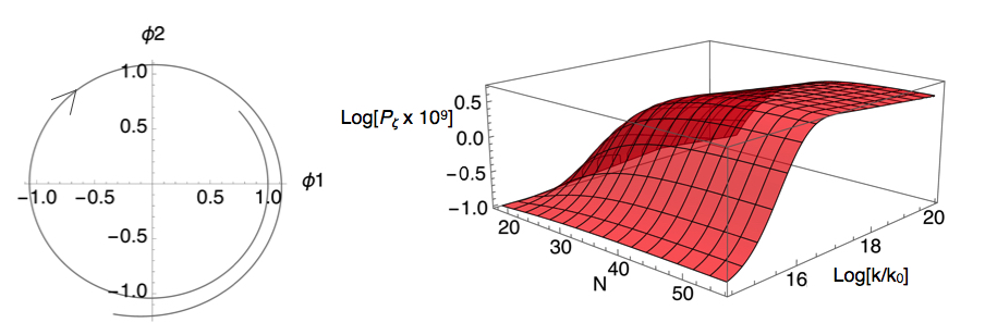
The dynamics of the inflaton is reminiscent of a person riding down a spiralling flume. Much like the person, the inflaton will sit close to the minimum in the radial direction, and will roll mainly along the angular direction. This deviation from the geodesics causes excitation of isocurvature modes and also transfers power from isocurvature perturbations to adiabatic perturbations, but this effect is only significant when the radial mass becomes sufficiently light. We therefore expect for scales exiting the horizon during the later stages when . Hence, by arranging for the radial mass to become lighter during the period when CMB scales are exiting the horizon, we ensure that smaller scales undergo a larger amount of superhorizon evolution than larger scales 1313 13 If this behaviour continues until the end of inflation, then the adiabatic limit will not be reached and hence the model is in principle sensitive to the details of reheating. We will not address this possibility here..
An example of this is shown in Fig. 8. The lefthand plot shows that although the minimum is at a fixed radius, the trajectory spirals outwards as a result of the decreasing mass. The righthand plot shows that at horizon exit the power spectrum is close to flat. This is a direct consequence of . We then see that smaller scales undergo a substantial amount of superhorizon evolution while large scales do not. This is because the isocurvature on the largest scales underwent a period of exponential decay and hence, even when the radial mass becomes light, isocurvature modes never grow to the extent that isocurvature modes exiting the horizon during the lighter phase do. The result is that by the end of inflation the spectrum does indeed appear suppressed on large scales.
7 Discussion
Observing statistically significant power suppression on the largest observable scales would require some non-minimal version of inflation and therefore radically improve the possibility of extracting valuable information about fundamental physics from the CMB. A number of authors have pointed out that a steepening of the potential associated with a tunnelling event can result in suppression of the power spectrum on large scales. Our paper extends this analysis by discussing the implications of this in the context of multifield inflation.
We find that the existence of a steepening along the inflationary direction is not a sufficient condition for power suppression, but rather that there is a relevant direction in field space that determines whether or not the power spectrum presents this suppression. This direction depends on the full inflationary trajectory in field space and is therefore not something determined locally from the potential. Furthermore, its orientation does not have to be aligned with the velocity vector in field space so fast evolution does not necessarily lead to power suppression even if it is present at horizon crossing. The reason for this behaviour is that the superhorizon evolution of isocurvature modes can source the adiabatic mode, thereby restoring its level of power after horizon crossing.
For models where the potential can be expressed as sum-separable, the situation becomes sufficiently simple such that it is possible to give analytic expressions for the constraints on the potential at horizon crossing to ensure large scale suppression of the power spectrum. This is further simplified in models where the adiabatic limit is reached shortly after the transition from the steep to the flat part of the potential where most of the e-folds of inflation would take place. We present simple 2-field models where we can easily visualise the dynamics and show explicit examples where the suppression at horizon crossing completely disappears after superhorizon evolution is taken into account. We also study the resultant power spectrum as a function of the parameters of the potential and initial conditions. This is important in the landscape picture where the initial conditions would be determined by an instanton that interpolates between the previous vacuum and the one described by this potential.
We also describe a novel approach to power suppression where the superhorizon evolution of perturbations plays a key role. One can envision a model where the relative power suppression is created by an enhancement of the level of the perturbations after the first few e-folds of inflation, in other words, one does not suppress the power at large scales but enhances it at small scales. We present a toy model that achieves this as a result of transfer of power from isocurvature to adiabatic perturbations over a prolonged period. This example may have interesting applications in inflationary models arising from compactification scenarios.
Our results have interesting implications for inflation in the landscape. If our observable patch emerged after tunnelling from a metastable vacua, then the combined conditions on the potential of the active fields and their initial conditions in order to achieve a suppressed large scale power spectrum imposes strong constraints on where in the landscape this event might have happened. In summary, observation of power suppression on large scales would enable one to establish a connection between the initial conditions for the onset of inflation in the landscape and the dynamics of active fields. We have made first steps in making this relationship precise.
8 Acknowledgements
The authors wish to thank Ana Achucarro, Pablo Ortiz, Yvette Welling and Jon Urrestilla for helpful discussions. J.J.B.-P. and JF are supported by IKERBASQUE, the Basque Foundation for Science. J.J.B.-P. is also supported in part by the Spanish Ministry of Science grant (FPA2012-34456) and Consolider EPI CSD2010-00064. KS acknowledges financial support from the University of the Basque Country UPV/EHU via the programme ÒAyudas de Especializacion al Personal Investigador (2012)Ó, from the Basque Government (IT-559-10), the Spanish Ministry (FPA2009-10612) and the Spanish Consolider-Ingenio 2010 Programme CPAN (CSD2007- 00042) and Consolider EPI CSD2010-00064. M. D. acknowledges support from the European Research Council under the European Unions Seventh Framework Programme (FP/20072013)/ERC Grant Agreement No. [308082]. We would particularly like to thank Baobab bar – teteria in Bilbao, where a significant portion of this work was done.
Appendix A Evolution of the scalar perturbations in the kinematical basis
In this appendix we will derive the equation for the scalar perturbations on superhorizon scales in the kinematic basis, where the evolution of curvature and isocurvature perturbations is explicit. We follow the notation of Refs. [62, 63, 64]. In these works, the curvature perturbation is defined in the comoving gauge and therefore denoted . Curvature perturbations defined in the constant density gauge — — and in the comoving gauge — — are known to be equal at second order on superhorizon scales up to corrections [67, 68]. For consistency with the standard usage of the separate universe assumption, in this paper, we will always refer to the curvature perturbation as .
For simplicity we will just discuss the case where the field space metric is flat everywhere, and therefore will not make any distinction between upper and lower indices. Moreover, we restrict ourselves to the slow-roll regime, where the background satisfies the equation
| (A.1) |
In particular we will show that curvature perturbations are conserved on superhorizon scales in the absence of entropy modes, and that curvature perturbations are not transferred into entropy modes. This two facts were used in § 2 to explain the simple structure of the transfer matrix in (2.2).
A.1 Equations for the scalar perturbations
As we discussed in § 2, scalar perturbations on superhorizon scales satisfy
| (A.2) |
The evolution of scalar perturbations becomes particularly simple when the perturbations are decomposed in the kinematic basis, , which is adapted to the background evolution. The basis vectors and (we use to refer to the element , not to be confused by an exponent 2) are defined as
| (A.3) |
The vector has unit norm since , and is defined to be a real positive number. The precise definitions of the rest of the basis vectors with will not be necessary for our derivation, and can be found in Ref. [64]. For our purposes it suffices to know that the full set forms an orthonormal basis, i.e. , where . As in the case of the vector , the evolution of the rest of the basis vectors along the inflationary trajectory is encoded in the elements of matrix
| (A.4) |
It is easy to check that this matrix is antisymmetric from the condition , which follows from the orthonormality of this set of vectors. In the kinematic basis the perturbations can be decomposed as
| (A.5) |
As we mentioned above, equations (A.2) become particularly clear when the perturbations are decomposed in this way, and this is due to the simple structure that the matrix has on the basis . To see this first note that from the background equation (A.1) we can derive the following two relations
| (A.6) |
Then, using and the definition for the basis vector (A.3), we can rewrite the second equation as
| (A.7) |
Projecting this relation along the vectors we find that the elements of the matrix in this basis satisfy
| (A.8) |
Finally, when the expression for the perturbations in the kinematic basis (A.5) is substituted into equation (A.2) we find
| (A.9) |
and after projecting this expression along the vectors and , we find that the curvature perturbations and isocurvature perturbations satisfy respectively
| (A.10) |
From this equations it is now clear that curvature perturbations are conserved in the absence of isocurvature pertubations, and that isocurvature is not sourced by curvature perturbations. It is straight forward to check that, when the second equation is written in terms of the entropy perturbations , it takes the form
| (A.11) |
A.2 The transfer matrix
The set of equations (A.10) and (A.11) can be written in matrix form as follows
| (A.12) |
The transfer matrix between two times labelled by the e-fold numbers is defined as
| (A.13) |
And therefore, the equation for the perturbations (A.12) implies that the transfer matrix between the times , and is given by
| (A.14) |
Since, by definition, transfer matrices satisfy the composition rule
| (A.15) |
the full transfer matrix can be obtained formally by multiplying a sequence of infinitesimal transfer matrices of the form (A.14). Moreover, as the composition preserves the upper triangular structure in (A.14) and also that , it follows that the structure of the full transfer mass matrix , has to be of the form
| (A.16) |
Appendix B Spectral index in multifield inflation
For convenience we define the transfer matrix as
| (B.1) |
which satisfies the same formal equation as
| (B.2) |
Transfer matrices satisfy the composition rule (A.15), which in particular implies that
| (B.3) |
Taking a derivative with respect to of the previous expression we find
| (B.4) |
Then, using the equation for (B.2), and projecting along the inflationary direction at the end of inflation, we arrive to
| (B.5) |
where we have defined . Finally, writing the power spectrum as
| (B.6) |
and given that the first equation also implies , we have
| (B.7) |
References
- (1) A. H. Guth, The Inflationary Universe: A Possible Solution to the Horizon and Flatness Problems, Phys.Rev. D23 (1981) 347–356.
- (2) K. Sato, First Order Phase Transition of a Vacuum and Expansion of the Universe, Mon.Not.Roy.Astron.Soc. 195 (1981) 467–479.
- (3) A. D. Linde, A New Inflationary Universe Scenario: A Possible Solution of the Horizon, Flatness, Homogeneity, Isotropy and Primordial Monopole Problems, Phys.Lett. B108 (1982) 389–393.
- (4) A. Albrecht and P. J. Steinhardt, Cosmology for Grand Unified Theories with Radiatively Induced Symmetry Breaking, Phys.Rev.Lett. 48 (1982) 1220–1223.
- (5) D. Baumann and L. McAllister, Inflation and String Theory, arXiv:1404.2601.
- (6) M. R. Douglas and S. Kachru, Flux compactification, Rev.Mod.Phys. 79 (2007) 733–796, [hep-th/0610102].
- (7) F. Denef, M. R. Douglas, and S. Kachru, Physics of String Flux Compactifications, Ann.Rev.Nucl.Part.Sci. 57 (2007) 119–144, [hep-th/0701050].
- (8) F. Denef, Les Houches Lectures on Constructing String Vacua, arXiv:0803.1194.
- (9) M. Grana, Flux compactifications in string theory: A Comprehensive review, Phys.Rept. 423 (2006) 91–158, [hep-th/0509003].
- (10) R. Bousso and J. Polchinski, Quantization of four form fluxes and dynamical neutralization of the cosmological constant, JHEP 0006 (2000) 006, [hep-th/0004134].
- (11) L. Susskind, The Anthropic landscape of string theory, hep-th/0302219.
- (12) S. R. Coleman and F. De Luccia, Gravitational Effects on and of Vacuum Decay, Phys.Rev. D21 (1980) 3305.
- (13) K. Yamamoto, M. Sasaki, and T. Tanaka, Large angle CMB anisotropy in an open universe in the one bubble inflationary scenario, Astrophys.J. 455 (1995) 412–418, [astro-ph/9501109].
- (14) M. Bucher and N. Turok, Open inflation with arbitrary false vacuum mass, Phys.Rev. D52 (1995) 5538–5548, [hep-ph/9503393].
- (15) J. Garriga, X. Montes, M. Sasaki, and T. Tanaka, Spectrum of cosmological perturbations in the one bubble open universe, Nucl.Phys. B551 (1999) 317–373, [astro-ph/9811257].
- (16) A. D. Linde, M. Sasaki, and T. Tanaka, CMB in open inflation, Phys.Rev. D59 (1999) 123522, [astro-ph/9901135].
- (17) D. Yamauchi, A. Linde, A. Naruko, M. Sasaki, and T. Tanaka, Open inflation in the landscape, Phys.Rev. D84 (2011) 043513, [arXiv:1105.2674].
- (18) J. Zhang, J. J. Blanco-Pillado, J. Garriga, and A. Vilenkin, Topological Defects from the Multiverse, 1501.05397.
- (19) A. Aguirre, M. C. Johnson, and A. Shomer, Towards observable signatures of other bubble universes, Phys.Rev. D76 (2007) 063509, [arXiv:0704.3473].
- (20) S. Chang, M. Kleban, and T. S. Levi, When worlds collide, JCAP 0804 (2008) 034, [arXiv:0712.2261].
- (21) A. Aguirre and M. C. Johnson, A Status report on the observability of cosmic bubble collisions, Rept.Prog.Phys. 74 (2011) 074901, [arXiv:0908.4105].
- (22) M. Kleban, Cosmic Bubble Collisions, Class.Quant.Grav. 28 (2011) 204008, [arXiv:1107.2593].
- (23) Planck Collaboration, P. Ade et al., Planck 2015 results. XIII. Cosmological parameters, arXiv:1502.01589.
- (24) M. Cicoli, G. Tasinato, I. Zavala, C. Burgess, and F. Quevedo, Modulated Reheating and Large Non-Gaussianity in String Cosmology, JCAP 1205 (2012) 039, [arXiv:1202.4580].
- (25) J. Frazer and A. R. Liddle, Exploring a string-like landscape, JCAP 1102 (2011) 026, [arXiv:1101.1619].
- (26) J. Frazer and A. R. Liddle, Multi-field inflation with random potentials: field dimension, feature scale and non-Gaussianity, JCAP 1202 (2012) 039, [arXiv:1111.6646].
- (27) N. Agarwal, R. Bean, L. McAllister, and G. Xu, Universality in D-brane Inflation, JCAP 1109 (2011) 002, [arXiv:1103.2775].
- (28) M. Dias, J. Frazer, and A. R. Liddle, Multifield consequences for D-brane inflation, JCAP 1206 (2012) 020, [arXiv:1203.3792].
- (29) J. Frazer, Predictions in multifield models of inflation, JCAP 1401 (2014), no. 01 028, [arXiv:1303.3611].
- (30) L. McAllister, S. Renaux-Petel, and G. Xu, A Statistical Approach to Multifield Inflation: Many-field Perturbations Beyond Slow Roll, JCAP 1210 (2012) 046, [arXiv:1207.0317].
- (31) R. Easther, J. Frazer, H. V. Peiris, and L. C. Price, Simple predictions from multifield inflationary models, Phys.Rev.Lett. 112 (2014) 161302, [arXiv:1312.4035].
- (32) T. C. Bachlechner, M. Dias, J. Frazer, and L. McAllister, Chaotic inflation with kinetic alignment of axion fields, Phys.Rev. D91 (2015), no. 2 023520, [arXiv:1404.7496].
- (33) L. C. Price, H. V. Peiris, J. Frazer, and R. Easther, Gravitational wave consistency relations for multifield inflation, Phys.Rev.Lett. 114 (2015), no. 3 031301, [arXiv:1409.2498].
- (34) WMAP Collaboration, G. Hinshaw et al., Nine-Year Wilkinson Microwave Anisotropy Probe (WMAP) Observations: Cosmological Parameter Results, Astrophys.J.Suppl. 208 (2013) 19, [arXiv:1212.5226].
- (35) Planck Collaboration, P. Ade et al., Planck 2015 results. XX. Constraints on inflation, arXiv:1502.02114.
- (36) C. R. Contaldi, M. Peloso, L. Kofman, and A. D. Linde, Suppressing the lower multipoles in the CMB anisotropies, JCAP 0307 (2003) 002, [astro-ph/0303636].
- (37) B. Feng and X. Zhang, Double inflation and the low cmb quadrupole, Phys.Lett. B570 (2003) 145–150, [astro-ph/0305020].
- (38) E. Dudas, N. Kitazawa, S. Patil, and A. Sagnotti, CMB Imprints of a Pre-Inflationary Climbing Phase, JCAP 1205 (2012) 012, [arXiv:1202.6630].
- (39) F. G. Pedro and A. Westphal, Low- CMB power loss in string inflation, JHEP 1404 (2014) 034, [arXiv:1309.3413].
- (40) R. Bousso, D. Harlow, and L. Senatore, Inflation after False Vacuum Decay: Observational Prospects after Planck, arXiv:1309.4060.
- (41) V. Miranda, W. Hu, and P. Adshead, Steps to Reconcile Inflationary Tensor and Scalar Spectra, Phys.Rev. D89 (2014), no. 10 101302, [arXiv:1403.5231].
- (42) D. K. Hazra, A. Shafieloo, G. F. Smoot, and A. A. Starobinsky, Ruling out the power-law form of the scalar primordial spectrum, JCAP 1406 (2014) 061, [arXiv:1403.7786].
- (43) K. M. Smith, C. Dvorkin, L. Boyle, N. Turok, M. Halpern, et al., Quantifying the BICEP2-Planck Tension over Gravitational Waves, Phys.Rev.Lett. 113 (2014), no. 3 031301, [arXiv:1404.0373].
- (44) D. K. Hazra, A. Shafieloo, G. F. Smoot, and A. A. Starobinsky, Inflation with Whip-Shaped Suppressed Scalar Power Spectra, Phys.Rev.Lett. 113 (2014), no. 7 071301, [arXiv:1404.0360].
- (45) R. Bousso, D. Harlow, and L. Senatore, Inflation After False Vacuum Decay: New Evidence from BICEP2, JCAP 1412 (2014), no. 12 019, [arXiv:1404.2278].
- (46) K. Kohri and T. Matsuda, Ambiguity in running spectral index with an extra light field during inflation, JCAP 1502 (2015), no. 02 019, [arXiv:1405.6769].
- (47) D. K. Hazra, A. Shafieloo, G. F. Smoot, and A. A. Starobinsky, Wiggly Whipped Inflation, JCAP 1408 (2014) 048, [arXiv:1405.2012].
- (48) M. Cicoli, S. Downes, B. Dutta, F. G. Pedro, and A. Westphal, Just enough inflation: power spectrum modifications at large scales, JCAP 1412 (2014), no. 12 030, [arXiv:1407.1048].
- (49) J. White, Y.-l. Zhang, and M. Sasaki, Scalar suppression on large scales in open inflation, Phys.Rev. D90 (2014), no. 8 083517, [arXiv:1407.5816].
- (50) R. K. Jain, P. Chingangbam, J.-O. Gong, L. Sriramkumar, and T. Souradeep, Punctuated inflation and the low CMB multipoles, JCAP 0901 (2009) 009, [arXiv:0809.3915].
- (51) R. K. Jain, P. Chingangbam, L. Sriramkumar, and T. Souradeep, The tensor-to-scalar ratio in punctuated inflation, Phys.Rev. D82 (2010) 023509, [arXiv:0904.2518].
- (52) C. R. Contaldi, M. Peloso, and L. Sorbo, Suppressing the impact of a high tensor-to-scalar ratio on the temperature anisotropies, JCAP 1407 (2014) 014, [arXiv:1403.4596].
- (53) B. Freivogel, M. Kleban, M. Rodriguez Martinez, and L. Susskind, Observational consequences of a landscape, JHEP 0603 (2006) 039, [hep-th/0505232].
- (54) J. J. Blanco-Pillado, M. Gomez-Reino, and K. Metallinos, Accidental Inflation in the Landscape, JCAP 1302 (2013) 034, [arXiv:1209.0796].
- (55) M. Dias, J. Frazer, and D. Seery, Computing observables in curved multifield models of inflation - A guide (with code) to the transport method, arXiv:1502.03125.
- (56) G. Rigopoulos and E. Shellard, The separate universe approach and the evolution of nonlinear superhorizon cosmological perturbations, Phys.Rev. D68 (2003) 123518, [astro-ph/0306620].
- (57) D. H. Lyth, K. A. Malik, and M. Sasaki, A General proof of the conservation of the curvature perturbation, JCAP 0505 (2005) 004, [astro-ph/0411220].
- (58) M. Sasaki and E. D. Stewart, A General analytic formula for the spectral index of the density perturbations produced during inflation, Prog.Theor.Phys. 95 (1996) 71–78, [astro-ph/9507001].
- (59) D. Wands, K. A. Malik, D. H. Lyth, and A. R. Liddle, A New approach to the evolution of cosmological perturbations on large scales, Phys.Rev. D62 (2000) 043527, [astro-ph/0003278].
- (60) D. H. Lyth and Y. Rodriguez, The Inflationary prediction for primordial non-Gaussianity, Phys.Rev.Lett. 95 (2005) 121302, [astro-ph/0504045].
- (61) D. Seery, D. J. Mulryne, J. Frazer, and R. H. Ribeiro, Inflationary perturbation theory is geometrical optics in phase space, JCAP 1209 (2012) 010, [arXiv:1203.2635].
- (62) C. M. Peterson and M. Tegmark, Testing Two-Field Inflation, Phys.Rev. D83 (2011) 023522, [arXiv:1005.4056].
- (63) C. M. Peterson and M. Tegmark, Non-Gaussianity in Two-Field Inflation, Phys.Rev. D84 (2011) 023520, [arXiv:1011.6675].
- (64) C. M. Peterson and M. Tegmark, Testing multifield inflation: A geometric approach, Phys.Rev. D87 (2013), no. 10 103507, [arXiv:1111.0927].
- (65) J.-O. Gong and T. Tanaka, A covariant approach to general field space metric in multi-field inflation, JCAP 1103 (2011) 015, [arXiv:1101.4809].
- (66) J. Elliston, D. Seery, and R. Tavakol, The inflationary bispectrum with curved field-space, JCAP 1211 (2012) 060, [arXiv:1208.6011].
- (67) K. A. Malik and D. Wands, Cosmological perturbations, Phys.Rept. 475 (2009) 1–51, [arXiv:0809.4944].
- (68) F. Vernizzi, On the conservation of second-order cosmological perturbations in a scalar field dominated Universe, Phys.Rev. D71 (2005) 061301, [astro-ph/0411463].
- (69) M. Dias, J. Elliston, J. Frazer, D. Mulryne, and D. Seery, The curvature perturbation at second order, JCAP 1502 (2015), no. 02 040, [arXiv:1410.3491].
- (70) S. Groot Nibbelink and B. van Tent, Density perturbations arising from multiple field slow roll inflation, hep-ph/0011325.
- (71) S. Groot Nibbelink and B. van Tent, Scalar perturbations during multiple field slow-roll inflation, Class.Quant.Grav. 19 (2002) 613–640, [hep-ph/0107272].
- (72) D. Wands, K. A. Malik, D. H. Lyth, and A. R. Liddle, A New approach to the evolution of cosmological perturbations on large scales, Phys.Rev. D62 (2000) 043527, [astro-ph/0003278].
- (73) D. Wands, N. Bartolo, S. Matarrese, and A. Riotto, An Observational test of two-field inflation, Phys.Rev. D66 (2002) 043520, [astro-ph/0205253].
- (74) C. Bennett, A. Banday, K. Gorski, G. Hinshaw, P. Jackson, et al., Four year COBE DMR cosmic microwave background observations: Maps and basic results, Astrophys.J. 464 (1996) L1–L4, [astro-ph/9601067].
- (75) D. Mulryne, D. Seery, and D. Wesley, Non-Gaussianity constrains hybrid inflation, arXiv:0911.3550.
- (76) D. J. Mulryne, D. Seery, and D. Wesley, Moment transport equations for the primordial curvature perturbation, JCAP 1104 (2011) 030, [arXiv:1008.3159].
- (77) D. J. Mulryne, Transporting non-Gaussianity from sub to super-horizon scales, JCAP 1309 (2013) 010, [arXiv:1302.3842].
- (78) C. Burgess, R. Easther, A. Mazumdar, D. F. Mota, and T. Multamaki, Multiple inflation, cosmic string networks and the string landscape, JHEP 0505 (2005) 067, [hep-th/0501125].
- (79) R. Allahverdi, A. Mazumdar, and T. Multamaki, Large tensor-to-scalar ratio and low scale inflation, arXiv:0712.2031.
- (80) F. Vernizzi and D. Wands, Non-gaussianities in two-field inflation, JCAP 0605 (2006) 019, [astro-ph/0603799].
- (81) T. Battefeld and R. Easther, Non-Gaussianities in Multi-field Inflation, JCAP 0703 (2007) 020, [astro-ph/0610296].
- (82) X. Chen, M.-x. Huang, S. Kachru, and G. Shiu, Observational signatures and non-Gaussianities of general single field inflation, JCAP 0701 (2007) 002, [hep-th/0605045].
- (83) A. Achucarro, J.-O. Gong, S. Hardeman, G. A. Palma, and S. P. Patil, Features of heavy physics in the CMB power spectrum, JCAP 1101 (2011) 030, [arXiv:1010.3693].
- (84) X. Chen, Primordial Features as Evidence for Inflation, JCAP 1201 (2012) 038, [arXiv:1104.1323].
- (85) X. Gao, D. Langlois, and S. Mizuno, Oscillatory features in the curvature power spectrum after a sudden turn of the inflationary trajectory, JCAP 1310 (2013) 023, [arXiv:1306.5680].
- (86) A. Achucarro, V. Atal, B. Hu, P. Ortiz, and J. Torrado, Inflation with moderately sharp features in the speed of sound: Generalized slow roll and in-in formalism for power spectrum and bispectrum, Phys.Rev. D90 (2014), no. 2 023511, [arXiv:1404.7522].
- (87) X. Chen and M. H. Namjoo, Standard Clock in Primordial Density Perturbations and Cosmic Microwave Background, Phys.Lett. B739 (2014) 285–292, [arXiv:1404.1536].
- (88) S. Mizuno, R. Saito, and D. Langlois, Combined features in the primordial spectra induced by a sudden turn in two-field DBI inflation, JCAP 1411 (2014), no. 11 032, [arXiv:1405.4257].
- (89) J. Martin and L. Sriramkumar, The scalar bi-spectrum in the Starobinsky model: The equilateral case, JCAP 1201 (2012) 008, [arXiv:1109.5838].
- (90) M. Cicoli, S. Downes, B. Dutta, F. G. Pedro, and A. Westphal, Just enough inflation: power spectrum modifications at large scales, JCAP 1412 (2014), no. 12 030, [arXiv:1407.1048].
- (91) T. Li, Z. Li, and D. V. Nanopoulos, Helical Phase Inflation, Phys.Rev. D91 (2015), no. 6 061303, [arXiv:1409.3267].
- (92) T. Li, Z. Li, and D. V. Nanopoulos, Helical Phase Inflation and Monodromy in Supergravity Theory, arXiv:1412.5093.