Photon Underproduction Crisis: Are QSOs sufficient to resolve it?

Photon Underproduction Crisis: Are QSOs sufficient to resolve it?–2015

Vikram Khaire ^†^†thanks: E-mail: vikramk@iucaa.ernet.in Raghunathan Srianand ^†^†thanks: E-mail: anand@iucaa.ernet.in Affiliation: IUCAA, Post Bag 4, Pune, India - 411007

Abstract

We investigate the recent claim of ‘photon underproduction crisis’ by Kollmeier et al. (2014) which suggests that the known sources of ultra-violet (UV) radiation may not be sufficient to generate the inferred H i photoionization rate ( $\Gamma_{\rm HI}$ ) in the low redshift inter-galactic medium. Using the updated QSO emissivities from the recent studies and our cosmological radiative transfer code developed to estimate the UV background, we show that the QSO contributions to $\Gamma_{\rm HI}$ is higher by a factor $\sim$ 2 as compared to the previous estimates. Using self-consistently computed combinations of star formation rate density and dust attenuation, we show that a typical UV escape fraction of 4% from star forming galaxies should be sufficient to explain the inferred $\Gamma_{\rm HI}$ by Kollmeier et al. (2014). Interestingly, we find that the contribution from QSOs alone can explain the recently inferred $\Gamma_{\rm HI}$ by Shull et al. (2015) which used the same observational data but different simulation. Therefore, we conclude that the crisis is not as severe as it was perceived before and there seems no need to look for alternate explanations such as low luminosity hidden QSOs or decaying dark matter particles.

Keywords:

Quasars, galaxies, intergalactic medium, diffuse radiation.

1 Introduction

Recently, Kollmeier et al. (2014, hereafter K14), used a cosmological hydrodynamic simulation together with the latest measurements of the H i column density distribution, $f(N_{\rm HI})$ , by Danforth et al. (2014) in the low- $z$ intergalactic medium (IGM) and reported a H i photoionization rate ( $\Gamma_{\rm HI}$ ) at $z=0$ . This is 5 times higher than the one (refer to as $\Gamma_{\rm HI}^{\rm HM}$ ) obtained from the theoretical estimates of cosmic ultraviolet background (UVB) by Haardt & Madau (2012, hereafter HM12). This apparent discrepancy has led to the claim of a ‘photon underproduction crisis’ suggesting that the origin of more than 80% of H i ionizing photons is unknown and perhaps generated from non-standard sources.

For a given sight-line in a cosmological simulation, the inferred $f(N_{\rm HI})$ depends on the assumed $\Gamma_{\rm HI}$ , the distribution of gas temperature and the clumping factor of the region producing the Ly- $\alpha$ absorption. The latter two quantities depend not only on the assumed initial power spectrum but also on various feedback processes that inject energy and momentum into the IGM from star forming galaxies. Therefore, the $\Gamma_{\rm HI}$ estimates using the $f(N_{\rm HI})$ will depend on how realistic the various feedbacks used in the simulation are. K14 have used the smooth particle hydrodynamics code gadget 2.0 (Springel, 2005) that includes feedback from galaxies in the form of momentum driven winds (Oppenheimer & Davé, 2008). However, Davé et al. (2010) suggested that these feedbacks produce negligible effect on $f(N_{\rm HI})$ for $N_{\rm HI}<10^{14}$ cm^-2.

Recently, Shull et al. (2015) have independently estimated $\Gamma_{\rm HI}$ , using the same observed data but simulated spectra obtained using the grid based Eulerian N-body hydrodynamics code enzo (Bryan et al., 2014). They found a smaller $\Gamma_{\rm HI}$ than K14 but it is still a factor 2 higher than $\Gamma_{\rm HI}^{\rm HM}$ . They attributed the decrease in the derived $\Gamma_{\rm HI}$ as compared to K14 to the differences in the implementations of feedback processes in the simulations used. While Shull et al. (2015) reduced the apparent tension, it still requires an appreciable contribution to the UVB from galaxies when one uses the previously estimated QSO emissivity.

In this study, we revisit the UVB calculations at $z\sim 0$ using the numerical radiative transfer code developed by us (Khaire & Srianand, 2013) in line with Faucher-Giguère et al. (2009) and HM12. We update the QSO and galaxy emissivity and show that the QSOs alone can provide the $\Gamma_{\rm HI}$ inferred by Shull et al. (2015) and to get the $\Gamma_{\rm HI}$ inferred by K14, we need only 4% of the ionizing photons to escape from galaxies (and not 15% as suggested by K14) . Throughout this paper we use a cosmology with $\Omega_{\Lambda}=0.7$ , $\Omega_{m}=0.3$ and $H_{0}=70$ km s^-1 Mpc^-1.

2 The radiative transfer

Following the standard procedure (Miralda-Escude & Ostriker, 1990; Shapiro et al., 1994; Haardt & Madau, 1996; Fardal et al., 1998; Shull et al., 1999), the average specific intensity, $J_{\nu_{0}}$ (in units of erg cm ${}^{\text{-2}}$ s ${}^{\text{-1}}$ Hz ${}^{\text{-1}}$ sr ${}^{\text{-1}}$ ), of the UVB at a frequency $\nu_{0}$ and redshift $z_{0}$ is given by,

J_{\nu_{0}}(z_{0})=\frac{1}{4\pi}\int_{z_{0}}^{\infty}dz\,\frac{dl}{dz}\,(1+z_{0})^{3}\,\epsilon_{\nu}(z)\,e^{-\tau_{\rm eff}(\nu_{0},z_{0},z)}.

(1)

Here, $\frac{dl}{dz}$ is the Friedmann-Lemaître-Robertson-Walker line element, $\epsilon_{\nu}(z)$ is the comoving specific emissivity of the sources and $\tau_{\rm eff}$ is an average effective optical depth encountered by photons of frequency $\nu_{0}$ at a redshift $z_{0}$ which were emitted from a redshift $z\,>z_{0}$ with a frequency $\nu\,>\nu_{0}$ . The frequency $\nu$ and $\nu_{0}$ are related by $\nu=\nu_{0}(1+z)/(1+z_{0})$ . Assuming that the IGM clouds of neutral hydrogen column density, $N_{\rm HI}$ , are Poisson-distributed along the line of sight, $\tau_{\rm eff}$ can be written as (Paresce et al., 1980, see),

\tau_{\rm eff}(\nu_{0},z_{0},z)=\int_{z_{0}}^{z}dz^{\prime}\int_{0}^{\infty}dN_{\rm HI}f(N_{\rm HI},z)(1-e^{-\tau_{\nu^{\prime}}})\,.

(2)

Here, $f(N_{\rm HI},z)$ is the number of H i clouds per unit redshift and column density interval having column density $N_{\rm HI}$ . The continuum optical depth $\tau_{\nu^{\prime}}$ is given by $\tau_{\nu^{\prime}}=N_{\rm HI}{\sigma_{\rm HI}(\nu^{\prime})}+N_{\rm HeI}{\sigma_{\rm HeI}(\nu^{\prime})}+N_{\rm HeII}{\sigma_{\rm HeII}(\nu^{\prime})},$ where, $N_{i}$ and $\sigma_{i}$ are the column density and photoionization cross-section, respectively, for species $i$ and $\nu^{\prime}=\nu_{0}(1+z^{\prime})/(1+z_{0})$ .

We use the same $f(N_{\rm HI},z)$ used by HM12 and neglect the contribution of He i to $\tau_{\nu}$ because of its negligible abundance at $z<6$ . We calculate $\tau_{\rm eff}$ following the prescription given in HM12. In the following section we provide the updated source emissivity.

Refer to caption — Figure 1: The $L_{\nu}\phi(L_{\nu})$ is plotted against M at g-band for two redshifts using various QLF reported in the literature. The area under each curve is proportional to the $\epsilon^{Q}_{g}$ (*left panel*). The $\epsilon^{Q}_{g}$ obtained for these QLFs, our $\epsilon^{Q}_{g}$ from the fit to the PD13 and C09 QLF (cyan points; see table 1 for details) and the $\epsilon^{Q}_{g}(z)$ inferred from $\epsilon^{Q}_{912}(z)$ of HM12 are also plotted (*right panel*). Here, the best fit PLE models of Boyle et al. (2000), Croom et al. (2004), with 2SLAQ data of Richards et al. (2005), C09 and PD13 and the luminosity dependent density evolution model of Bongiorno et al. (2007) are used.

3 Emissivity of radiating sources

We calculate the UVB assuming only QSOs and galaxies are sources of the UV radiation. Therefore, $\epsilon_{\nu}(z)=\epsilon^{Q}_{\nu}(z)+\epsilon_{\nu}^{G}(z)$ where $\epsilon^{Q}_{\nu}(z)$ and $\epsilon_{\nu}^{G}(z)$ are the comoving specific emissivity from QSOs and galaxies, respectively.

3.1 Comoving QSO emissivity

The $\epsilon^{Q}_{\nu}(z)$ , in units of erg s^-1 Hz^-1 Mpc^-3, using the observed QSO luminosity function (QLF) at a frequency $\nu$ is given by

\epsilon^{Q}_{\nu}(z)=\int_{L_{\nu}^{min}}^{\infty}{L_{\nu}(z)\phi(L_{\nu},z)dL_{\nu}}\,,

(3)

where, $\phi(L_{\nu},z)$ is the QLF at $z$ given in terms of specific luminosity $L_{\nu}$ by

\phi(L_{\nu})=(\phi_{L}^{*}/L^{*})\,[\,(L_{\nu}/L^{*})^{-\gamma_{1}}+(L_{\nu}/L^{*})^{-\gamma_{2}}\,]^{-1},

(4)

and using the absolute AB magnitudes, M, by

\phi(M)={\phi_{M}^{*}}[{10^{0.4(\gamma_{1}+1)(M-M^{*})}+10^{0.4(\gamma_{2}+1)(M-M^{*})}}]^{-1},

(5)

where $\phi_{M}^{*}=0.921\phi_{L}^{*}$ . We use $L_{\nu}^{min}=0.01L^{*}$ to calculate the $\epsilon^{Q}_{\nu}$ . Note that, for most of the QLFs at $z<3.5$ the faint end slope $\gamma_{1}\geq-1.4$ (see Table 2), for which the value of $\epsilon^{Q}_{\nu}$ is insensitive to the values of $L_{\nu}^{min}<0.01L^{*}$ . For example, the maximum difference in the $\epsilon^{Q}_{\nu}$ calculated for $L_{\nu}^{min}=0$ and $0.01L^{*}$ is less than 5% for $\gamma_{1}\geq-1.4$ and $\gamma_{2}=-3.5$ .

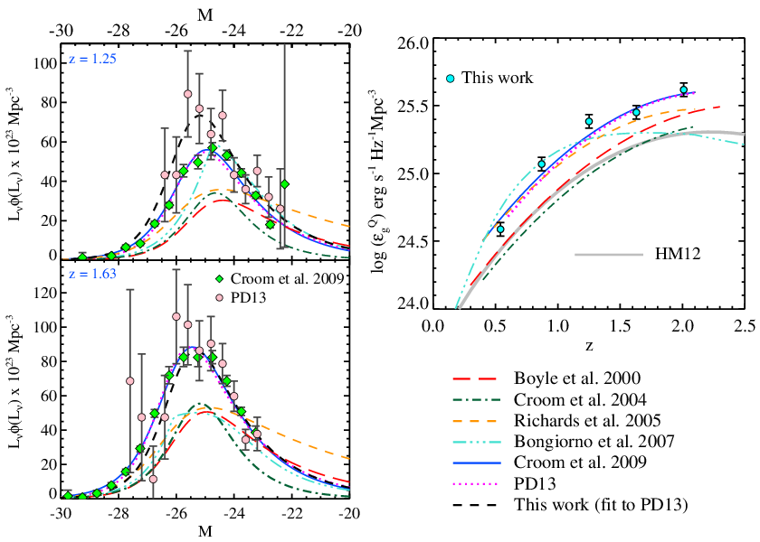
In Fig.1 (left panel), we plot the $L_{\nu}\phi(L_{\nu})$ estimates against $g$ -band magnitudes from various studies at two different $z$ . The area under each curve is proportional to the respective emissivity at $g$ -band ( $\epsilon^{Q}_{g}$ ). It is clear from the Fig.1 that, as compared to old QLF measurements of Boyle et al. (2000) and Croom et al. (2004), using the new measurements of Croom et al. (2009, hereafter C09) and Palanque-Delabrouille et al. (2013, hereafter PD13) will give a larger $\epsilon^{Q}_{g}$ . This is indeed the case, as demonstrated in the right panel of Fig.1 where we plot the $\epsilon^{Q}_{g}$ for these QLF measurements. We have also plotted the $\epsilon^{Q}_{g}$ converted from the $\epsilon^{Q}_{912}(z)$ given at the H i Lyman limit (i.e at 912Å) by HM12 using the relation $\log(\epsilon^{Q}_{g})=\log(\epsilon^{Q}_{912})+0.487$ which is consistent with the spectral energy distribution (SED) used by HM12. This $\epsilon^{Q}_{g}$ is consistent with Boyle et al. (2000) and Croom et al. (2004) which is smaller by factor $\sim$ 1.5 to 2 as compared to C09 and PD13.

In our study, we use the latest QLF measurements as summarized in Table 1. The first and second columns give the reference and the wavelength ( $\lambda_{\rm band}$ ) at which the QLF is reported, respectively. For $0.3<z<3.5$ , in each redshift bin we fit the observed QLF with the form given in Eq. 5 using an idl mpfit routine by fixing the values of $\gamma_{1}$ and $\gamma_{2}$ to those reported in the respective references (our fits are also presented in Fig 1). We use our best fit $\phi^{*}_{M}$ and $M^{*}$ to obtain $\epsilon_{\lambda{\rm band}}(z)$ (see Table 1). At other redshifts, we take the best fit QLF parameters given in the respective references and calculate the $\epsilon^{Q}_{\lambda{\rm band}}(z)$ . In Fig 1 (right panel), we show that the $\epsilon^{Q}_{g}(z)$ at $z<2$ obtained using our fit is consistent with the pure luminosity evolution (PLE) models of PD13 and C09.

We convert the $\epsilon^{Q}_{\lambda{\rm band}}(z)$ into $\epsilon^{Q}_{912}(z)$ using the broken power law QSO SED $\rm L_{\nu}\propto\nu^{-\alpha}$ , which we adopt for our UVB calculations. In the soft X-ray regime above energy 0.5 keV ( $\lambda\leq\rm 24.8\AA$ ) we use $\alpha=0.9$ (Nandra & Pounds, 1994). Following Stevans et al. (2014), we use $\alpha=1.4$ for $24.8<\lambda\leq\rm 1000\AA~$ ¹¹ 1 Stevans et al. (2014) found $\alpha=1.41\pm 0.15$ using QSO composite spectrum down to about 500Å. We extrapolate it upto $\lambda\sim 25\rm\AA$ . Note that the UVB at $\lambda<500\rm\AA$ has negligible contribution to $\Gamma_{\rm HI}$ . and $\alpha=0.8$ for $1000<\lambda\leq\rm 2000\AA$ . For $\lambda>\rm 2000\AA$ we use $\alpha=0.5$ .

For the observed QLF at $z<3.5$ , the SEDs used to perform continuum $K$ -corrections in the original references ( $\rm L_{\nu}\propto\nu^{-\alpha^{\prime}}$ ; $\alpha^{\prime}$ is given in the last column of Table 1) are different from our adopted SED at $\lambda\geq 1500$ Å. For consistency, we recompute the specific emissivity $\epsilon^{Q}_{\lambda{\rm rest}}(z)$ at $\lambda_{\rm rest}=\lambda_{\rm band}/(1+z)$ using $\alpha^{\prime}$ from the corresponding reference and then use our adopted SED to convert $\epsilon^{Q}_{\lambda{\rm rest}}(z)$ in to $\epsilon^{Q}_{912}(z)$ . This is not needed for $z\geq 4$ where the QLFs are obtained at 1450Å in the QSO’s rest frame using appropriately matched filters without applying additional $K$ -corrections. The errors on the $\epsilon^{Q}_{912}(z)$ given in the Table 1 are the maximum and minimum difference we get using the errors in $\gamma_{1}$ and $\gamma_{2}$ given in original references except at $z=0.15$ . In this case the error on $\epsilon^{Q}_{912}$ is the difference we get in $\epsilon^{Q}_{912}$ if we use $L_{\nu}^{min}=0.1$ and 0.001.

All our $\epsilon^{Q}_{912}(z)$ measurements as a function of $z$ are plotted in Fig. 2. We fit these points using a functional form similar to that of HM12 and obtain the following best fit,

\epsilon^{Q}_{912}(z)=10^{24.6}\,(1+z)^{5.9}\,\frac{\exp(-0.36z)}{\exp(2.2z)+25.1}\,\,.

(6)

For comparison, in Fig.2, we show this best fit ${\epsilon^{Q}_{912}(z)}$ along with the ${\epsilon^{Q}_{912}(z)}$ used by HM12. For $z<3.5$ , our ${\epsilon^{Q}_{912}(z)}$ is higher than that of HM12 and the maximum difference of factor 2.1 occurs at $z\sim 1.5$ . The peak in ${\epsilon^{Q}_{912}(z)}$ also changes from $z=2.2$ from HM12 to $z=1.95$ . In Fig. 2, we also show the $\epsilon^{Q}_{912}(z)$ obtained using the PLE models of C09 and PD13 and the luminosity evolution and density evolution (LEDE) model of Ross et al. (2013). These are consistent with our fit in Eq.6. Note that the PLE models of C09 and PD13 give identical values of $\epsilon^{Q}_{g}(z)$ (see right panel of Fig.1) but differ slightly in the $\epsilon^{Q}_{912}(z)$ since they use different SED for continuum $K$ -correction (see Table 1).

3.2 Comoving galaxy emissivity

In Khaire & Srianand (2014, hereafter KS14), by matching the observed galaxy emissivity from multi-band, multi-epoch galaxy luminosity functions, we have determined self-consistent combinations of the star formation rate density (SFRD) and dust attenuation magnitude in the FUV band ( $A_{\rm FUV}$ ) for five well known extinction curves. It has been found that the SFRD( $z$ ) and $A_{\rm FUV}(z)$ estimated using the average extinction curve of the Large Magellanic Cloud Supershell (LMC2) is consistent with various observations.

Here, as our fiducial model, we use the $\epsilon^{G}_{\nu}(z)$ computed from the SFRD( $z$ ) and $A_{\rm FUV}(z)$ obtained in KS14 for the LMC2 extinction curve (see tables 2 and 4 in KS14). Our SFRD at $z<0.5$ is a factor $\sim 3$ higher than that of HM12 (Madau & Dickinson, 2014, see also). However, the difference decreases at higher $z$ , and becomes less than 10% at $z\sim 3$ . A small fraction, $f_{\rm esc}$ , of the generated H i ionizing photons ( $\lambda<912$ Å) from the stellar population are assumed to escape through holes in galaxies (i.e by assuming that dust does not modify the SED at $\lambda<912$ Å). We assume that there are no He ii ionizing photons ( $\lambda\leq 228$ Å) escaping the galaxy. This is a reasonable assumption in the $z$ -range of our interest. We approximate the galaxy emissivity at $\lambda<912$ Å with a power-law $\epsilon^{G}_{\nu}\propto\nu^{-1.8}$ . The exponent is fixed to reproduce the $\Gamma_{\rm HI}$ obtained from the model spectrum itself. Note that the exponent and the total H i ionizing photons generated inside the galaxy depends on the metallicity, initial mass function (IMF), stellar rotation rates and adopted evolutionary tracks (Topping & Shull, 2015, see). In our galaxy models obtained from starburst99 (Leitherer et al., 1999), we use the Salpeter IMF with $0.4$ times solar metallicity. See KS14 for a discussion on the uncertainties in estimating SFRD( $z$ ) and $A_{\rm FUV}(z)$ arising from the assumed metallicity and IMF.

In addition to this, we have also included some of the diffuse emission from the IGM clouds. We model the He ii Ly- $\alpha$ and He ii Balmer continuum recombination emission following the prescription given in HM12 and the Lyman continuum emission due to recombination of H i and He ii using the approximations given in Faucher-Giguère et al. (2009). We do not include the contributions to UVB from He i recombinations and the two photon continuum. These contributions are negligible, and if included, can increase $\Gamma_{\rm HI}$ by a maximum of 10% (Faucher-Giguère et al., 2009). We also do not include the resonance absorption of Heii which has a negligible effect on $\Gamma_{\rm HI}$ , especially at low- $z$ (see HM12).

4 Results and Discussions

Here, we focus on the H i photoionization rate, $\Gamma_{\rm HI}$ , obtained using our UVB model. This is defined as

\Gamma_{\rm HI}=\int_{\nu_{\rm HI}}^{\infty}d\nu\,\frac{4\pi J_{\nu}}{h\nu}\,\sigma_{\rm HI}(\nu)\,,

(7)

where $\nu_{\rm HI}$ corresponds to $\lambda=912$ Å. In Fig. 3, we summarize various available $\Gamma_{\rm HI}$ measurements as a function of $z$ . In particular, denoting $\Gamma_{\rm HI,13}=\Gamma_{\rm HI}\times 10^{13}~s^{-1}$ , the points of interest for the present study are $\Gamma_{\rm HI,13}\sim 1.8$ at $z=0.1$ as inferred by Kollmeier et al. (2014) which led to the claim of a ‘photon underproduction crisis’ and the very recent estimates of $\Gamma_{\rm HI,13}(z)=0.46(1+z)^{4.4}$ at $z<0.5$ found by Shull et al. (2015).

To begin with, we validate our code by reproducing the results of HM12. In Fig 3, we plot the $\Gamma_{\rm HI}(z)$ determined by HM12 (long dashed curve) and the result of our code obtained using the $\epsilon^{Q}_{\nu}(z)$ , SED and $f_{\rm esc}$ used by HM12 (dotted curve). Both match with each other within $\sim 5$ % accuracy. The minor differences noticed can be attributed to the different metallicities used and contributions of some of the diffuse emission processes ignored in our model. Having validated our code, we use the updated QSO emissivity $\epsilon^{Q}_{912}(z)$ (see Eq. 6) and the $\epsilon^{G}_{\nu}(z)$ mentioned above (in Section 3.2) to calculate the UVB (and hence $\Gamma_{\rm HI}$ ) for different values of $f_{\rm esc}$ .

When we use only the QSOs as the source of the UVB (by taking $f_{\rm esc}=0$ ) and use our updated $\epsilon^{Q}_{\nu}(z)$ , we get the $\Gamma_{\rm HI}$ at $z<0.5$ very close (i.e within 10%) to the values predicted by Shull et al. (2015) and Shull et al. (2014). We find that the one-sided ionizing flux $\Phi_{0}$ , as defined in Shull et al. (2015) is to be $5030$ cm^-2 s^-1 for our UVB at $z=0$ as compared to 5700 cm^-2 s^-1 obtained by Shull et al. (2015). However, because of the statistical uncertainties in the observed $f(N_{\rm HI})$ , the $\Gamma_{\rm HI}$ and $\Phi_{0}$ predicted by Shull et al. (2015) can be even higher. Our $\Gamma_{\rm HI,13}$ values are 0.41, 0.94, 1.9 and 3.3 at $z=0$ , 0.2, 0.4 and 0.6, respectively. These are $\sim$ 2 times higher than the corresponding $\Gamma_{\rm HI}^{\rm HM}$ values. Now, instead of using our $\epsilon^{Q}_{\nu}(z)$ fitting form, if we take the best fit PLE models given in C09 and PD13 (see Fig 2) for $z<2.2$ , and estimate the UVB by assuming $\epsilon^{Q}_{912}(z)=0$ at $z>2.2$ , we get the $\Gamma_{\rm HI,13}$ at $z=0$ to be 0.48 and 0.39, respectively. It shows that, irrespective of our QLF fits and the fitting form, the updated QSO emissivity will lead to $\Gamma_{\rm HI}\sim 1.7$ to $2.1\times\Gamma_{\rm HI}^{\rm HM}$ . Therefore, we conclude that the $\Gamma_{\rm HI}$ inferred by Shull et al. (2014) and Shull et al. (2015) can be explained by the QSOs alone without requiring any significant contribution from the galaxies (i.e with $f_{\rm esc}=0$ ). This is consistent with many low- $z$ upper limits on average $f_{\rm esc}$ measured in samples of galaxies (Siana et al., 2007; Cowie et al., 2009; Siana et al., 2010; Bridge et al., 2010; Leitet et al., 2013). Therefore, there is no real photon underproduction crisis when we consider the $\Gamma_{\rm HI}$ measurements of Shull et al. (2015).

In our UVB calculations with $f_{\rm esc}=0$ , we use a different QSO SED and an updated $\epsilon^{Q}_{\nu}(z)$ as compared to HM12. However, since the $\Gamma_{\rm HI}\propto(3+\alpha)^{-1}$ , changing $\alpha$ from 1.57 (HM12) to 1.4 at $\lambda<912$ Å increases the $\Gamma_{\rm HI}$ by only 4%. The main difference in $\Gamma_{\rm HI}$ between our UVB and that of HM12 arises because of the updated $\epsilon^{Q}_{\nu}(z)$ . It is important to realize that even though the $\epsilon^{Q}_{912}$ used by us matches with $\epsilon^{Q}_{912}$ of HM12 at $z=0$ , the local UVB is contributed more by ionizing photons coming from high- $z$ , up to $z\sim 2$ , where the mean free path for H i ionizing photons is very large and $\epsilon^{Q}_{912}(z)$ peaks.

Next we explore the $f_{\rm esc}$ requirements in order to reproduce the $\Gamma_{\rm HI}$ inferred by Kollmeier et al. (2014). For simplicity we run models keeping $f_{\rm esc}$ constant over the full $z$ range. We find $f_{\rm esc}=4\%$ is needed to get the $\Gamma_{\rm HI,13}=1.8$ at $z=0.1$ (see Fig 3). Interestingly, the $f_{\rm esc}$ needed in our calculations is much less than the $f_{\rm esc}=15\%$ required in the HM12 UVB model. Apart from 2 times higher QSO emissivity, it is partly because of our $\sim$ 3 times higher low- $z$ SFRD as compared to HM12. Note that, the value of $f_{\rm esc}\sim 0.02$ % used by HM12 to estimate UVB at $z=0.1$ is extremely small compared to various low- $z$ observations. In passing, we note that for our models with different combinations of SFRD and $A_{\rm FUV}$ explored for different extinction curves in KS14, we require $f_{\rm esc}$ values similar to or less than what we have obtained here for our fiducial model.

In order to compare with observations, we use a relative escape fraction, $f_{\rm esc,rel}$ , defined as $f_{\rm esc,rel}=f_{\rm esc}\times 10^{0.4A_{\rm FUV}}$ . To match the $\Gamma_{\rm HI}$ of K14, the model of HM12 that assumes $A_{\rm FUV}=1$ at $z<2$ , will require $f_{\rm esc,rel}=38\%$ while we need only $f_{\rm esc,rel}=15\%$ for our fiducial LMC2 model at $z=0$ (where we determined $A_{\rm FUV}=1.42$ ). This $f_{\rm esc,rel}=15\%$ is about a factor $\sim 2$ higher than the low $z$ upper limits on $f_{\rm esc,rel}$ given in various studies of galaxy samples as mentioned above. However the $f_{\rm esc}$ observed in individual galaxies (Borthakur et al., 2014) and many theoretical estimates (Kimm & Cen, 2014; Roy et al., 2014, e.g.) are consistent with it. Therefore, we conclude that with the updated QSO and galaxy emissivities presented here, even if we wish to generate $\Gamma_{\rm HI}$ inferred by K14, the required $f_{esc}$ of ionizing photons from star forming galaxies is not abnormally high enough to warrant an alternate non-standard source of the UVB.

Interestingly, our updated QSO emissivity alone can reproduce the $\Gamma_{\rm HI}$ measurements at high $z$ (Bolton & Haehnelt, 2007; Becker & Bolton, 2013) up to $z\sim 2.7$ . However, $f_{\rm esc}=4\%$ gives a $\Gamma_{\rm HI}(z)$ which marginally overestimates the $\Gamma_{\rm HI}$ measurements at $2<z<3$ (see Fig.3). Irrespective of the low- $z$ $\Gamma_{\rm HI}$ , at $z>3$ one needs galaxies to contribute more to the UVB (Giallongo et al., 2015, however see,). At high- $z$ , using the observations of H i and He ii Ly- $\alpha$ forest, it will be possible to constraints the $f_{\rm esc}$ from galaxies (Khaire & Srianand, 2013, see,). We plan to do this in the near future.

Column (4) gives $\phi^{*}$ in units Mpc^-3 mag^-1, column (5) gives M^∗ in AB magnitudes and column (8) and (9) gives $\epsilon^{Q}_{\nu}$ in units erg s^-1 Hz^-1 Mpc^-3. The $\lambda_{\rm band}$ at 1450Å, 4450Å, 4686Å and 7480Å corresponds to FUV, B, $g$ and $i$ band, respectively. ^⋆We assume $\alpha^{\prime}=0.5$ consistent with the $k$ -correction of Schulze et al. (2009). ^†PD13 stands for Palanque-Delabrouille et al. (2013). ^‡NA indicates that the $K$ -correction is not applied.

Table 1: Details of observed QLF used to get

\epsilon^{Q}_{912}

in our study.

Reference	$\lambda_{\rm band}$	z	log $\phi^{*}$	M^∗	$\gamma_{1}$	$\gamma_{2}$	log $\epsilon^{Q}_{\lambda_{\rm band}}$	log $\epsilon^{Q}_{912}$	$\alpha^{\prime}$
(1)	(2)	(3)	(4)	(5)	(6)	(7)	(8)	(9)	(10)
Schulze et al. (2009)	4450Å	0.15	-4.81	-19.46	-2.0	-2.82	24.30	23.83 $\pm 0.20$	0.5^⋆
Croom et al. (2009)	4686Å	0.54	-5.98	-24.10	-1.4 $\pm 0.1$	-3.5 $\pm 0.1$	24.59	24.14 $\pm 0.05$	0.3
PD13 ${}^{{}^{\dagger}}$	4686Å	0.87	-5.74	-24.68	-1.4 $\pm 0.1$	-3.5 $\pm 0.1$	25.07	24.59 $\pm 0.05$	0.5
		1.25	-5.81	-25.65			25.38	24.90 $\pm 0.05$
		1.63	-5.80	-25.80			25.45	24.98 $\pm 0.05$
		2.01	-6.00	-26.71			25.62	25.17 $\pm 0.05$
Ross et al. (2013)	7480Å	2.25	-5.83	-26.45	-1.3 ${}^{+0.5}_{-0.2}$	-3.5 ${}^{+0.3}_{-0.2}$	25.64	25.06 ${}^{+0.11}_{-0.16}$	0.5
		2.35	-5.98	-26.55			25.53	24.95 ${}^{+0.11}_{-0.16}$
		2.45	-6.12	-26.81			25.50	24.91 ${}^{+0.11}_{-0.16}$
		2.55	-6.12	-26.77			25.47	24.89 ${}^{+0.11}_{-0.16}$
		2.65	-6.21	-27.06			25.51	24.92 ${}^{+0.11}_{-0.16}$
		2.75	-6.26	-27.27			25.54	24.96 ${}^{+0.11}_{-0.16}$
		2.90	-6.29	-27.22			25.49	24.91 ${}^{+0.11}_{-0.16}$
		3.12	-6.38	-27.13			25.36	24.79 ${}^{+0.11}_{-0.16}$
		3.37	-6.66	-27.63			25.29	24.72 ${}^{+0.11}_{-0.16}$
Glikman et al. (2011)	1450Å	4.0	-5.89	-24.10	-1.6 ${}^{+0.8}_{-0.6}$	-3.3 $\pm 0.2$	24.80	24.62 ${}^{+0.50}_{-0.30}$	NA^‡
Masters et al. (2012)	1450Å	4.25	-7.12	-25.64	-1.72 $\pm 0.28$	-2.6 $\pm 0.63$	24.32	24.13 ${}^{+0.50}_{-0.22}$	NA
McGreer et al. (2013)	1450Å	5.0	-8.47	-27.21	-2.03 ${}^{+0.15}_{-0.14}$	-4.0	23.78	23.60 ${}^{+0.15}_{-0.14}$	NA
Kashikawa et al. (2015)	1450Å	6.0	-8.92	-26.91	-1.92 ${}^{+0.24}_{-0.19}$	-2.81	23.13	22.94 $\pm 0.15$	NA

5 Summary

The recent claim of a ‘photon underproduction crisis’ (Kollmeier et al., 2014) requires the low- $z$ $\Gamma_{\rm HI}$ to be 5 times higher than the one obtained by the UVB model of HM12. A similar investigation performed by Shull et al. (2015) finds a lower $\Gamma_{\rm HI}$ which is still 2 times higher than that of HM12. Here, we present an updated H i ionizing QSO emissivity by using recent QLF measurements. It turns out that this emissivity is a factor of 1.5 to 2 times higher than what is used by HM12 at $0.5<z<2.5$ . We estimate the UVB using this emissivity with the help of a radiative transfer code developed by us. We show that QSOs alone can give a factor 2 required by Shull et al. (2015). Using our updated SFRD which is $\sim$ 3 times higher than HM12 at low- $z$ , to get the $\Gamma_{\rm HI}$ predicted by Kollmeier et al. (2014) we require only 4% of the ionizing photons generated by galaxies to escape into the IGM. Therefore, there is no need to look for additional sources of ionizing photons such as hidden QSOs or decaying dark matter particles.

acknowledgments

We thank M. Shull, D. Weinberg, F. Haardt, A. Paranjape, T. R. Choudhury and H. Padmanabhan for useful comments on the manuscript. VK acknowledges support from CSIR.

References

Adams et al. (2011) Adams J. J., Uson J. M., Hill G. J., MacQueen P. J., 2011, ApJ, 728, 107
Becker & Bolton (2013) Becker G. D., Bolton J. S., 2013, MNRAS, 436, 1023
Bolton & Haehnelt (2007) Bolton J. S., Haehnelt M. G., 2007, MNRAS, 382, 325
Bongiorno et al. (2007) Bongiorno A. et al., 2007, A&A, 472, 443
Borthakur et al. (2014) Borthakur S., Heckman T. M., Leitherer C., Overzier R. A., 2014, Science, 346, 216
Boyle et al. (2000) Boyle B. J., Shanks T., Croom S. M., Smith R. J., Miller L., Loaring N., Heymans C., 2000, MNRAS, 317, 1014
Bridge et al. (2010) Bridge C. R. et al., 2010, ApJ, 720, 465
Bryan et al. (2014) Bryan G. L. et al., 2014, ApJS, 211, 19
Cowie et al. (2009) Cowie L. L., Barger A. J., Trouille L., 2009, ApJ, 692, 1476
Croom et al. (2004) Croom S. M., Smith R. J., Boyle B. J., Shanks T., Miller L., Outram P. J., Loaring N. S., 2004, MNRAS, 349, 1397
Croom et al. (2009) Croom S. M. et al., 2009, MNRAS, 399, 1755
Danforth et al. (2014) Danforth C. W. et al., 2014, ArXiv e-prints 1402.2655
Davé et al. (2010) Davé R., Oppenheimer B. D., Katz N., Kollmeier J. A., Weinberg D. H., 2010, MNRAS, 408, 2051
Fardal et al. (1998) Fardal M. A., Giroux M. L., Shull J. M., 1998, AJ, 115, 2206
Faucher-Giguère et al. (2008) Faucher-Giguère C. A., Prochaska J. X., Lidz A., Hernquist L., Zaldarriaga M., 2008, ApJ, 681, 831
Faucher-Giguère et al. (2009) Faucher-Giguère C. A., Lidz A., Zaldarriaga M., Hernquist L., 2009, ApJ, 703, 1416
Giallongo et al. (2015) Giallongo E. et al., 2015, ArXiv e-prints 1502.02562
Glikman et al. (2011) Glikman E., Djorgovski S. G., Stern D., Dey A., Jannuzi B. T., Lee K. S., 2011, ApJ, 728, L26
Haardt & Madau (1996) Haardt F., Madau P., 1996, ApJ, 461, 20
Haardt & Madau (2012) Haardt F., Madau P., 2012, ApJ, 746, 125
Kashikawa et al. (2015) Kashikawa N. et al., 2015, ApJ, 798, 28
Khaire & Srianand (2013) Khaire V., Srianand R., 2013, MNRAS, 431, L53
Khaire & Srianand (2014) Khaire V., Srianand R., 2014, ApJ, in press (arXiv:1405.7038)
Kimm & Cen (2014) Kimm T., Cen R., 2014, ApJ, 788, 121
Kollmeier et al. (2014) Kollmeier J. A. et al., 2014, ApJ, 789, L32
Leitet et al. (2013) Leitet E., Bergvall N., Hayes M., Linné S., Zackrisson E., 2013, A&A, 553, A106
Leitherer et al. (1999) Leitherer C. et al., 1999, ApJS, 123, 3
Madau & Dickinson (2014) Madau P., Dickinson M., 2014, AR&A, 52, 415
Masters et al. (2012) Masters D. et al., 2012, ApJ, 755, 169
McGreer et al. (2013) McGreer I. D. et al., 2013, ApJ, 768, 105
Miralda-Escude & Ostriker (1990) Miralda-Escude J., Ostriker J. P., 1990, ApJ, 350, 1
Nandra & Pounds (1994) Nandra K., Pounds K. A., 1994, MNRAS, 268, 405
Oppenheimer & Davé (2008) Oppenheimer B. D., Davé R., 2008, MNRAS, 387, 577
Palanque-Delabrouille et al. (2013) Palanque-Delabrouille N. et al., 2013, A&A, 551, A29
Paresce et al. (1980) Paresce F., McKee C. F., Bowyer S., 1980, ApJ, 240, 387
Richards et al. (2005) Richards G. T. et al., 2005, MNRAS, 360, 839
Ross et al. (2013) Ross N. P. et al., 2013, ApJ, 773, 14
Roy et al. (2014) Roy A., Nath B. B., Sharma P., 2014, ArXiv e-prints 1412.7924
Schulze et al. (2009) Schulze A., Wisotzki L., Husemann B., 2009, A&A, 507, 781
Shapiro et al. (1994) Shapiro P. R., Giroux M. L., Babul A., 1994, ApJ, 427, 25
Shull et al. (1999) Shull J. M., Roberts D., Giroux M. L., Penton S. V., Fardal M. A., 1999, AJ, 118, 1450
Shull et al. (2014) Shull J. M., Danforth C. W., Tilton E. M., 2014, ApJ, 796, 49
Shull et al. (2015) Shull J. M., Moloney J., Danforth C. W., Tilton E. M., 2015, ArXiv e-prints 1502.00637
Siana et al. (2007) Siana B. et al., 2007, ApJ, 668, 62
Siana et al. (2010) Siana B. et al., 2010, ApJ, 723, 241
Springel (2005) Springel V., 2005, MNRAS, 364, 1105
Stevans et al. (2014) Stevans M. L., Shull J. M., Danforth C. W., Tilton E. M., 2014, ApJ, 794, 75
Topping & Shull (2015) Topping M. W., Shull J. M., 2015, ApJ, 800, 97