A randomized blocked algorithm for efficiently computing rank-revealing factorizations of matrices
Per-Gunnar Martinsson and Sergey Voronin
Department of Applied Mathematics, University of Colorado at Boulder
Abstract: This manuscript describes a technique for computing partial rank-revealing factorizations, such as, e.g, a partial QR factorization or a partial singular value decomposition. The method takes as input a tolerance and an matrix , and returns an approximate low rank factorization of that is accurate to within precision in the Frobenius norm (or some other easily computed norm). The rank of the computed factorization (which is an output of the algorithm) is in all examples we examined very close to the theoretically optimal -rank. The proposed method is inspired by the Gram-Schmidt algorithm, and has the same asymptotic flop count. However, the method relies on randomized sampling to avoid column pivoting, which allows it to be blocked, and hence accelerates practical computations by reducing communication. Numerical experiments demonstrate that the accuracy of the scheme is for every matrix that was tried at least as good as column-pivoted QR, and is sometimes much better. Computational speed is also improved substantially, in particular on GPU architectures.
1. Introduction
1.1. Problem formulation
This manuscript describes an algorithm based on randomized sampling for computing an approximate low-rank factorization of a given matrix. To be precise, given a real or complex matrix of size , and a computational tolerance , we seek to determine a matrix of low rank such that
| (1) |
For any given , a rank- approximation to that is in many ways optimal is given by the partial singular value decomposition (SVD),
| (2) |
where and are orthonormal matrices whose columns consist of the first left and right singular vectors, respectively, and is a diagonal matrix whose diagonal entries are the leading singular values of , ordered so that . The Eckart-Young theorem [3] states that for the spectral norm and the Frobenius norm, the residual error is minimal,
However, computing the factors in (2) is computationally expensive. In contrast, our objective is to find an approximant that is cheap to compute, and close to optimal.
The method we present is designed for situations where is sufficiently large that computing the full SVD is not economical. The method is designed to be highly communication efficient, and to execute efficiently on both shared and distributed memory machines. It has been tested numerically for situations where the matrix fits in RAM on a single machine. We will, without loss of generality, assume that . For the most part we discuss real matrices, but the generalization to complex matrices is straight-forward.
1.2. A greedy template
A standard approach in computing low-rank factorizations is to employ a greedy algorithm to build, one vector at a time, an orthonormal basis that approximately spans the columns of . To be precise, given an matrix and a computational tolerance , our objective is to determine a rank , and an matrix with orthonormal column vectors such that , where . The matrices and may be constructed jointly via the following procedure:
Algorithm 1 (1) ; ; ; ; (2) while (3) (4) Pick a unit vector . (5) (6) (7) (8) (9) end while (10) .
Note that can overwrite . It can be verifiedthat if the algorithm is executed in exact arithmetic, then the matrices generated satisfy
| (3) |
The performance of the greedy scheme is determined by how we choose the vector on line (4). If we pick as simply the largest column of , scaled to yield a vector of unit length, then we recognize the scheme as the column pivoted Gram-Schmidt algorithm for computing a QR factorization. This method often works very well, but can lead to sub-optimal factorizations. Reference [5] discusses this in detail, and also provides an improved pivoting technique that can be proved to yield closer to optimal results. However, both standard Gram-Schmidt (see, e.g., [4, Sect. 5.2]), and the improved version in [5] are challenging to implement efficiently on modern multicore processors since they cannot readily be blocked. Expressed differently, they rely on BLAS2 operations rather than BLAS3.
Another natural choice for on line (4) is to pick the unit vector that minimizes . This in fact leads to an optimal factorization, with the vectors being left singular vectors of . However, finding the minimizer tends to be computationally expensive.
In this manuscript, we propose a scheme that is more computationally efficient than column-pivoted Gram-Schmidt, and often yields close to minimal approximation errors. The idea is to choose as a random linear combination of the columns of . To be precise, we propose the following mechanism for choosing :
(4a) Draw a random vector whose entries are iid Gaussian random variables. (4b) Set . (4c) Normalize so that .
This scheme is mathematically very close to the low-rank approximation scheme proposed in [6], but is slightly different in the stopping criterion used (the scheme of [6] does not explicitly update the matrix, and therefore relies on a probabilistic stopping criterion), and in its performance when executed with finite precision arithmetic. We argue that choosing the vector using randomized sampling leads to performance very comparable to traditional column pivoting, but has a decisive advantage in that the resulting algorithm is easy to block. We will demonstrate substantial practical speed-up on both multicore CPUs and GPUs.
Remark 1.
The factorization scheme described in this section produces an approximate factorization of the form , where is orthonormal, but no conditions are à priori imposed on . Once the factors and are available, it is simple to compute many standard factorizations such as the low rank QR, SVD, or CUR factorizations. For details, see Section 3.3.
2. Technical preliminaries
2.1. Notation
Throughout the paper, we measure vectors in using their Euclidean norm. The default norm for matrices will be the Frobenius norm , although other norms will also be discussed.
We use the notation of Golub and Van Loan [4] to specify submatrices. In other words, if is an matrix with entries , and and are two index vectors, then we let denote the matrix
We let denote the matrix , and define analogously.
The transpose of is denoted , and we say that a matrix is orthonormal if its columns form an orthonormal set, so that .
2.2. The singular value decomposition (SVD)
The SVD was introduced briefly in the introduction. Here we define it again, with some more detail added. Let denote an matrix, and set . Then admits a factorization
| (4) |
where the matrices and are orthonormal, and is diagonal. We let and denote the columns of and , respectively. These vectors are the left and right singular vectors of . As in the introduction, the diagonal elements of are the singular values of . We order these so that . We let denote the truncation of the SVD to its first terms, as defined by (2). It is easily verified that
| (5) |
where denotes the operator norm of and denotes the Frobenius norm of . Moreover, the Eckart-Young theorem [3] states that these errors are the smallest possible errors that can be incurred when approximating by a matrix of rank .
2.3. The QR factorization
Any matrix admits a QR factorization of the form
| (6) |
where , is orthonormal, is upper triangular, and is a permutation matrix. The permutation matrix can more efficiently be represented via a vector of column indices such that where is the identity matrix. Then (6) can be written
| (7) |
The QR-factorization is often computed via column pivoting combined with either the Gram-Schmidt process, Householder reflectors, or Givens rotations [4]. The resulting upper triangular then satisfies various decay conditions [4]. These techniques are all incremental, and can be stopped after the first terms have been computed to obtain a “partial QR-factorization of ”:
| (8) |
The main drawback of the classical partial pivoted QR approximation is the difficulty to obtain substantial speedups on multi-processor architectures.
2.4. Orthonormalization
Given an matrix , with , we introduce the function
to denote orthonormalization of the columns of . In other words, will be an orthonormal matrix whose columns form a basis for the column space of . In practice, this step is typically achieved most efficiently by a call to a packaged QR factorization (e.g., in Matlab, we would write ). This step could in principle be implemented without pivoting, which makes this call efficient.
3. Construction of low-rank approximations via randomized sampling
3.1. A basic randomized scheme
Let be a given matrix whose singular values exhibit some decay, and suppose that we seek a matrix with orthonormal columns such that
| (9) |
In other words, we seek a matrix whose columns form an approximate orthonormal basis for the column space of . A randomized procedure for solving this task was proposed in [7], and later analyzed an elaborated in [8, 6]. A basic version of the scheme that we call “randQB” is given in Figure 1. Once randQB has been executed to produce the factors and in (9), standard factorizations such as the QR factorization, or the truncated SVD can easily be obtained, as described in Section 3.3.
function (1) (2) (3)
3.2. Over sampling and theoretical performance guarantees
The algorithm randQB described in Section 3.1 produces close to optimal results for matrices whose singular values decay rapidly, provided that some slight over-sampling is done. To be precise, if we seek to match the minimal error for a factorization of rank , then choose in randQB as
where is a small integer (say ). It was shown in [6, Thm. 10.5] that if , then
where denotes expectation. Recall from equation (5) that is the theoretically minimal error in approximating by a matrix of rank , so we miss the optimal bound only by a factor of (except for the over sampling, of course). Moreover, it can be shown that the likelihood of a substantial deviation from the expectation is extremely small [6, Sec. 10.3].
Remark 2.
When errors are measured in the spectral norm, as opposed to the Frobenius norm, the randomized scheme is slightly further removed from optimality. Theorem 10.6 of [6] states that
| (10) |
where is the basis of the natural exponent. We observe that in cases where the singular values decay slowly, the right hand side of (10) is substantially larger than the theoretically optimal value of . For such situation, the “power scheme” described in Section 5.1 should be used.
3.3. Computing standard factorizations
The output of the randomized factorization scheme in Figure 1 is a factorization where is orthonormal, but no constraints have been placed on . It turns out that standard factorizations can efficiently be computed from the factors and ; in this section we describe how to get the QR, the SVD, and “interpolatory” factorizations.
3.3.1. Computing the low rank SVD
To get a low rank SVD, cf. Section 2.2, we perform the full SVD on the matrix , to obtain a factorization . Then,
We can now choose a rank to use based on the decaying singular values of . Once a suitable rank has been chosen, we form the low rank SVD factors:
so that . Observe that the truncation undoes the over-sampling that was done and detects a numerical rank that is typically very close to the optimal -rank.
3.3.2. Computing the partial pivoted QR factorization
To obtain the factorization , cf. Section 2.3, from the QB decomposition, perform a QR factorization of the matrix to obtain . Then, set to obtain
3.3.3. Computing interpolatory and CUR factorizations
In applications such as data interpretation, it is often of interest to determine a subset of the rows/columns of that form a good basis for its row/column space. For concreteness, suppose that is an matrix of rank , and that we seek to determine an index set of length , and a matrix of size such that
| (11) |
One can prove that there always exist such a factorization for which every entry of is bounded in modulus by (which is to say that the columns in form a well-conditioned basis for the range of ) and for which is the identity matrix [2]. Now suppose that we have available a factorization where is of size . Then determine and such that
| (12) |
This can be done using the techniques in, e.g., [2] or [5]. Then (11) holds automatically for the index set and the matrix that were constructed. Using similar ideas, one can determine a set of rows that form a well-conditioned basis for the row space, and also the so called CUR factorization
where and consist of subsets of the columns and rows of , respectively, cf. [12].
4. A blocked version of the randomized range finder
In this section, we describe and analyze a blocked version of the basic randomized scheme described in Figure 1. By blocking, we improve computational efficiency and simplify implementation on parallel machines. Blocking also allows for adaptive rank determination to be incorporated for situations where the rank is not known in advance. While blocking greatly helps with computational efficiency, it also creates some issues in terms of aggregation of round-off errors; this problem can be eliminated using techniques described in Section 4.3.
The algorithm described in this section is directly inspired by Algorithm 4.2 of [6]; besides blocking, the scheme proposed here is different in that the matrix is updated in a manner analogous to “modified” column-pivoted Gram-Schmidt. This updating allows the randomized stopping criterion employed in [6] to be replaced with a precise deterministic stopping criterion.
4.1. Blocking
Converting the basic scheme in Figure 1 to a blocked scheme is in principle straight-forward. Suppose that in addition to an matrix and a rank , we have set a block size such that , for some integer . Then draw an Gaussian random matrix , and partition it into slices , each of size , so that
| (13) |
We analogously partition the matrices and in groups of columns and rows, respectively,
The blocked algorithm then proceeds to build the matrices and one at a time. We first initiate the algorithm by setting
| (14) |
Then step forwards, computing for the matrices
| (15) | ||||
| (16) | ||||
| (17) |
We will next prove that the matrix constructed is indeed orthonormal, and that the matrix defined by (17) is the “remainder” after steps, in the sense that
To be precise, we will prove the following proposition:
Proposition 4.1.
Let be an matrix. Let denote a block size, and let denote the number of steps. Suppose that the rank of is at least . Let be a Gaussian random matrix of size , partitioned as in (13), with each of size . Let , , and , be defined by (14) – (17). Set:
| (18) |
and
| (19) |
Then for every , it is the case that:
- (a)
The matrix is ON, so is an orthogonal projection.
- (b)
and .
- (c)
.
Proof.
The proof is by induction. We will several times use that if is a matrix of size of full rank, and we set , then , where denotes the range of . We will also use the fact that if is a Gaussian random matrix of size , and is a matrix of size with rank at least , then the rank of is with probability 1 precisely [6].
Direct inspection of the definitions show that (a), (b), (c) are all true for . Suppose all statements are true for . We will prove that then (a), (b), (c) hold for .
To prove that (a) holds for , we use that (b) holds for and insert this into (15) to get
| (20) |
Then observe that is the orthogonal projection onto a space of dimension , which means that the matrix has rank at least . Consequently, has rank precisely . This shows that
It follows that whenever which shows that is ON. Next,
It follows that:
Thus, (a) holds for .
Proving (b) is a simple calculation. Combining (16) and (17) we get
where in the last step we used that . Since , this proves (b).
To prove (c), we observe that (20) implies that
| (21) |
Induction assumption (c) tells us that
| (22) |
Combining (21) and (22), we find
| (23) |
Equation (23) together with the induction assumption (c) imply that . But both of these spaces have dimension precisely , so the fact that one is a subset of the other implies that they must be identical.∎
Let us next compare the blocked algorithm defined by relations (14) – (17) to the unblocked algorithm described in Figure 1. Let for a fixed Gaussian matrix , the output of the blocked version be and let the output of the unblocked method be . These two pairs of matrices do not need to be identical. (They depend on how exactly the QR factorizations are implemented, for instance). However, Proposition 4.1 demonstrates that the projectors and are identical. To be precise, both of these matrices represent the orthogonal projection onto the space . This means that the error resulting from the two algorithms are also identical
Consequently, all theoretical results given in [6], cf. Section 3.2, directly apply to the output of the blocked algorithm too.
4.2. Adaptive rank determination
The blocked algorithm defined by (14) – (17) was in Section 4.1 presented for the case where the rank of the approximation is given in advance. A perhaps more common situation in practical applications is that a precision is specified, and then we seek to compute an approximation of as low rank as possible that is accurate to precision . Observe that in the algorithm defined by (14) – (17), we proved that after step has been completed, we have
In other words, holds precisely the residual remaining after step . This means that incorporating adaptive rank determining is now trivial — we simply compute after completing step , and break once . The algorithm resulting is shown as randQB_b in Figure 2. (The purpose of line (3’) will be explained in Section 4.3.)
Remark 3.
Recall that our default norm in this manuscript, the Frobenius norm, is simple to compute, which means that the check on whether to break the loop on line (7) in Figure 2 hardly adds at all to the execution time. If circumstances warrant the use of a norm that is more expensive to compute, then some modification of the algorithm would be required. Suppose, for instance, that we seek an approximation in the spectral norm. We could then use the fact that the Frobenius norm is an upper bound on the spectral norm, keep the Frobenius norm as the breaking condition, and then eliminate any “superfluous” degrees of freedom that were included in the post-processing step, cf. Section 3.3.1. (This approach would only be practicable for matrices whose singular values exhibit reasonable decay, as otherwise the discrepancy in the -ranks would be prohibitively large.)
4.3. Floating point arithmetic
When the algorithm defined by (14) – (17) is carried out in finite precision arithmetic, a serious problem often arises in that round-off errors will accumulate and will cause loss of orthonormality among the columns in . The problem is that as the computation proceeds, the columns of each computed matrix will due to round-off errors drift into the span of the columns of . To fix this problem, we explicitly reproject away from the span of the previously computed basis vectors [1]. The line (3’) in Figure 2 represents the re-projection that is done to combat the accumulation of round-off errors. (Note that if the algorithm is carried out in exact arithmetic, then whenever , so line (3’) would have no effect.)
function (1) for (2) (3) (3’) (4) (5) (6) if then stop (7) end for (8) Set and .
4.4. Comparison of execution times
Let us compare the computational cost of algorithms randQB (Figure 1) and randQB_b (Figure 2). To this end, let and denote the scaling constants for the cost of executing a matrix-matrix multiplication and a full QR factorization, respectively. (While the algorithms only need the function orth, cf. Section 2.4, this cost is for practical purposes the same as the cost for QR factorization.) In other words, we assume that:
- •
Multiplying two matrices of sizes and costs .
- •
Performing a QR factorization of a matrix of size , with , costs .
Note that these are rough estimates. Actual costs depend on the actual sizes (note that the costs are dominated by data movement rather than flops), but this model is still instructive. The execution time for the algorithm in Figure 1 is easily seen to be
| (24) |
For the blocked algorithm of Figure 2, we assume that it stops after steps and set . Then
Using that we find
| (25) |
Comparing (24) and (25), we see that the blocked algorithm involves one additional term of , but on the other hand spends less time executing full QR factorizations, as expected.
Remark 4.
All blocked algorithms that we present share the characteristic that they slightly increase the amount of time spent on matrix-matrix multiplication, while reducing the amount of time spent performing QR factorization. This is a good trade-off on many platforms, but becomes particularly useful when the algorithm is executed on a GPU. These massively multicore processors are particularly efficient at performing matrix-matrix multiplications, but struggle with communication intensive tasks such as a QR factorization.
5. A version of the method with enhanced accuracy
5.1. Randomized sampling of a power of the matrix
The accuracy of the basic randomized approximation scheme described in Section 3, and the blocked version of Section 4 is well understood. The analysis of [6] (see the synopsis in Section 3.2) shows that the error depends strongly on the quantity . This implies that the scheme is highly accurate for matrices whose singular values decay rapidly, but less accurate when the “tail” singular values have substantial weight. The problem becomes particularly pronounced for large matrices. Happily, it was demonstrated in [9] that this problem can easily be resolved when given a matrix with slowly decaying singular values by simply applying a power of the matrix to be analyzed to the random matrix. To be precise, suppose that we are given an matrix , a target rank , and a small integer (say or ). Then the following formula will produce an ON matrix whose columns form an approximation to the range:
The key observation here is that the matrix has exactly the same left singular values as , but its singular values are (observe that our objective is to build an ON-basis for the range of , and the optimal such basis consists of the leading left singular vectors). Even a small value of will typically provide enough decay that highly accurate results are attained. For a theoretical analysis, see [6, Sec. 10.4].
When the “power scheme” idea is to be executed in floating point arithmetic, substantial loss of accuracy happens whenever the singular values of have a large dynamic range. To be precise, if denotes the machine precision, then any singular components smaller than will be lost. This problem can be resolved by orthonormalizing the “sample matrix” between each application of and . This results in the scheme we call randQB_p, as shown in Figure 3. (Note that this scheme is virtually identical to a classical subspace iteration with a random Gaussian matrix as the start [10].)
function (1) . (2) . (3) for (4) . (5) . (6) end for (7)
5.2. The blocked version of the power scheme
A blocked version of randQB_p is easily obtained by a process analogous to the one described in Section 4.1, resulting in the algorithm “randQB_pb” in Figure 4. Line (8) combats the problem of incremental loss of orthonormality when the algorithm is executed in finite precision arithmetic, cf. Section 4.3.
function (1) for (2) . (3) . (4) for (5) . (6) . (7) end for (8) (9) (10) (11) if then stop (12) end while (13) Set and .
5.3. Computational complexity
When comparing the computational cost of randQB_p (cf. Figure 3) versus randQB_pb (cf. Figure 4), we use the notation that was introduced in Section 4.4. By inspection, we directly find that
For the blocked scheme, inspection tells us that
Executing the sum, and utilizing that , we get
In other words, the blocked algorithm again spends slightly more time executing matrix-matrix multiplications, and quite a bit less time on qr-factorizations. This trade is often favorable, and particularly so when the algorithm is executed on a GPU (cf. Remark 4). On the other hand, when , the benefit to saving time on QR factorizations is minor.
5.4. Is re-orthonormalizing truly necessary?
Looking at algorithm randQB_p, it is very tempting to skip the intermediate QR factorizations and simply execute steps (2) – (6) as:
(2) . (3) for (4) . (5) end for (6)
This simplification does speed things up substantially, but as we mentioned earlier, it can lead to loss of accuracy. In this section we state some conjectures about when re-orthonormalization is necessary. These conjectures appear to show that the blocked scheme is much more resilient to skipping re-orthonormalization.
To describe the issue, let us fix a (small) integer , and define the matrix
If the SVD of is , then the SVD of is
In computing , we lose all information about any singular mode for which , where is the machine precision. In other words, in order to accurately resolve the first singular modes, re-orthogonalization is needed if
| (26) |
As an example, with and , we find that , so re-orthonormalization is imperative resolve any components smaller than . Moreover, if we skip re-orthonormalization, we are likely to see an overall loss of accuracy affecting singular values and singular vectors associated with larger singular values.
Next consider the blocked scheme. The crucial observation is that now, instead of trying to extract the whole range of singular values (and their associated eigenvectors) at once, we now extract them in groups of modes each, where . This means that we can expect to get reasonable accuracy as long as
| (27) |
Comparing (26) and (27), we see that (27) is a much milder condition, in particular when the block size is much smaller than .
All claims in this section are heuristics. However, while they have not been rigorously proven, they are supported by extensive numerical experiments, see Section 6.3.
6. Numerical experiments
In this section, we present numerical examples that illustrate the computational efficiency and the accuracy of the proposed scheme, see Sections 6.1 and 6.2, respectively. The codes we used are available at http://amath.colorado.edu/faculty/martinss/main_codes.html and we encourage any interested reader to try the methods out, and explore different parameter sets than those included here.
6.1. Comparison of execution speeds
We first compare the run times of different techniques for computing a partial (rank ) QR factorization of a given matrix of size . Observe that the choice of matrix is immaterial for a run time comparison (we investigate accuracy in Section 6.2). We compared three sets of techniques:
- •
Truncating a full QR factorization, computed using the Intel MKL libraries.
- •
Taking steps of a column pivoted Gram-Schmidt process. The implementation was accelerated by using MKL library functions whenever practicable.
- •
The blocked “QB” scheme, followed by postprocessing of the factors to obtain a QR factorization. We used the “power method” described in Section 5 with parameters .
The algorithms were all implemented in C and run on a desktop with a 6-core Intel Xeon E5-1660 CPU (3.30 GHZ), and 128GB of RAM. We also ran the blocked “QB” scheme on an NVIDIA Tesla K40c GPU installed on the same machine, using the Matlab GPU computing interface. The results are shown in Figure 5. Figure 6 shows the dependence of the runtime on the block size.
Figure 5 shows that our blocked algorithms (blue, magenta, and cyan lines) compare favorably to both of the two benchmarks we chose — full QR using MKL libraries (green) and partial factorization using column pivoting (green). However, it must be noted that our implementation of column pivoted QR is far slower than the built-in QR factorization in the MKL libraries. Even for as low of a rank as , we do not break even with a full factorization until . This implies that column pivoting can be implemented far more efficiently than we were able to. The point is that in order to attain the efficiency of the MKL libraries, very careful coding that is customized to any particular computing platform would have to be done. In contrast, our blocked code is able to exploit the very high efficiency of the MKL libraries with minimal effort.
Finally, it is worth nothing how particularly efficient our blocked algorithms are when executed on a GPU. We gain a substantial integer factor speed-up over CPU speed in every test we conducted.
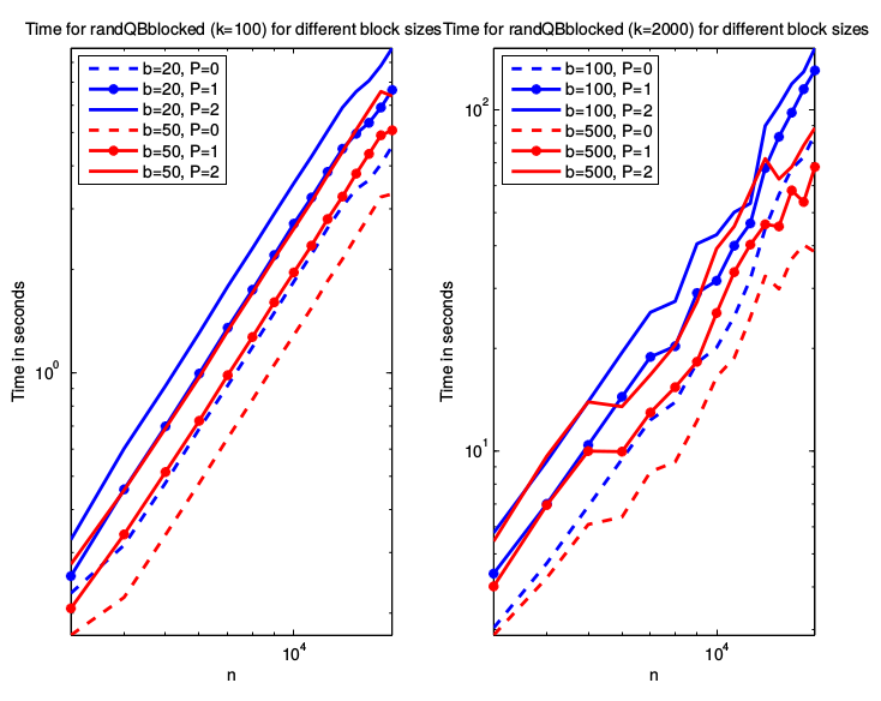
6.2. Accuracy of the randomized scheme
We next investigate the accuracy of the randomized schemes versus column-pivoted QR on the one hand (easy to compute, not optimal) and versus the truncated SVD on the other (expensive to compute, optimal). We used 5 classes of test matrices that each have different characteristics:
- Matrix 1 (fast decay):
-
Let denote an matrix of the form where and are randomly drawn matrices with orthonormal columns (obtained by performing qr on a random Gaussian matrix), and where is a diagonal matrix with entries roughly given by where is a random number drawn from a uniform distribution on and . To precision , the rank of is about 75.
- Matrix 2 (slow decay):
-
The matrix is formed just like , but now the diagonal entries of decay very slowly, with .
- Matrix 3 (sparse):
-
The matrix is a sparse matrix given by where and are random sparse vectors generated by the Matlab commands and , respectively. We used and with resulted in a matrix with roughly non-zero elements. This matrix was borrowed from Sorensen and Embree [11] and is an example of a matrix for which column pivoted Gram-Schmidt performs particularly well.
- Matrix 4 (Kahan):
-
This is a variation of the “Kahan counter-example” which is a matrix designed so that Gram-Schmidt performs particularly poorly. The matrix here is formed via the matrix matrix product where:
with random . Then is upper triangular, and for many choices of and , classical column pivoting will yield poor performance as the different column norms will be similar and pivoting will generally fail. The rank- approximation resulting from column pivoted QR is substantially less accurate than the optimal rank- approximation resulting from truncating the full SVD [5]. However, we obtain much better results than QR with the QB algorithm.
- Matrix 5 (S shaped decay):
-
The matrix is built in the same manner as and , but now the diagonal entries of are chosen to first hover around 1, then decay rapidly, and then level out at a relatively high plateau, cf. Figure 11.
We compare four different techniques for computing a rank- approximation to our test matrices:
- SVD:
-
We computed the full SVD (using the Matlab command svd) and then truncated to the first components.
- Column-pivoted QR:
-
We implemented this using modified Gram-Schmidt with reorthogonalization to ensure that orthonormality is strictly maintained in the columns of .
- randQB — single vector:
-
This is the greedy algorithm labeled “Algorithm 1” in Section 1.2, implemented with on line (4) chosen as where and where is a random Gaussian vector.
- randQB — blocked:
-
This is the algorithm randQB_pb shown in Figure 4.
The results are shown in Figure 7 – 11. We make three observations: (1) When the “power method” described in Section 5 is used, the accuracy of randQB_pb exceeds that of column-pivoted QR in every example we tried, even for as low of a power as . (2) Blocking appears to lead to no loss of accuracy. In most cases, there is no discernible difference in accuracy between the blocked and the non-blocked versions. (3) The accuracy of randQB_pb is particularly good when errors are measured in the Frobenius norm. In almost all cases we investigated, essentially optimal results are obtained even for .
Figures 7 – 11 report the errors resulting from a single instantiation of the randomized algorithm. Appendix A provides more details on the statistical distribution of errors.
6.3. When re-orthonormalization is required
We claimed in Section 5.4 that the blocked scheme is more robust towards loss of orthonormality than the non-blocked scheme presented in [6]. To test this hypothesis, we tested what happens if we skip the re-orthonormalization between applications of and in the algorithms shown in Figures 3 and 4. The results are shown in Figure 12. The key observation here is that the blocked versions of randQB still always yield excellent precision. When the block size is large, the convergence is slowed down a bit compared to the more meticulous implementation, but essentially optimal accuracy is nevertheless obtained relatively quickly.
Remark 5.
The numerical results in Figure 12 substantiate the claim that for the unblocked version, the best accuracy attainable is . In all examples, we have , so the prediction is that for the maximum precision is and for it is . The results shown precisely follow this pattern. Observe that for , no loss of accuracy is seen at all since the singular values we are interested in level out at about .
7. Concluding remarks
We have described a randomized algorithm for the low rank approximation of matrices. The algorithm is based on the randomized sampling paradigm described in [7, 9, 6, 8]. In this article, we introduce a blocking technique which allows us to incorporate adaptive rank determination without sacrificing computational efficiency, and an updating technique that allows us to replace the randomized stopping criterion proposed in [6] with a deterministic one. Through theoretical analysis and numerical examples, we demonstrate that while the blocked scheme is mathematically equivalent to the non-blocked scheme of [7, 9, 6, 8] when executed in exact arithmetic, the blocked scheme is slightly more robust towards accumulation of round-off errors.
The updating strategy that we propose is directly inspired by a classical scheme for computing a partial QR factorization via the column pivoted Gram-Schmidt process. We demonstrate that the randomized version that we propose is more computationally efficient than this classical scheme (since it is hard to block the column pivoting scheme). Our numerical experiments indicate that the randomized version not only improves speed, but also leads to higher accuracy. In fact, in all examples we present, the errors resulting from the blocked randomized scheme are very close to the optimal error obtained by truncating a full singular value decomposition. In particular, when errors are measured in the Frobenius norm, there is almost no loss of accuracy at all compared to the optimal factorization, even for matrices whose singular values decay slowly.
The scheme described can output any of the standard low-rank factorizations of matrices such as, e.g., a partial QR or SVD factorization. It can also with ease produce less standard factorizations such as the “CUR” and “interpolative decompositions (ID)”, cf. Section 3.3.
Acknowledgements: The research reported was supported by DARPA, under the contract N66001-13-1-4050, and by the NSF, under the contract DMS-1407340.
References
- [1] A. Björck, Numerics of Gram-Schmidt orthogonalization, Linear Algebra Appl. 197/198 (1994), 297–316, Second Conference of the International Linear Algebra Society (ILAS) (Lisbon, 1992). MR 1275620 (95b:65060)
- [2] H. Cheng, Z. Gimbutas, P.G. Martinsson, and V. Rokhlin, On the compression of low rank matrices, SIAM Journal of Scientific Computing 26 (2005), no. 4, 1389–1404.
- [3] Carl Eckart and Gale Young, The approximation of one matrix by another of lower rank, Psychometrika 1 (1936), no. 3, 211–218.
- [4] Gene H. Golub and Charles F. Van Loan, Matrix computations, fourth ed., Johns Hopkins Studies in the Mathematical Sciences, Johns Hopkins University Press, Baltimore, MD, 2013. MR 3024913
- [5] Ming Gu and Stanley C. Eisenstat, Efficient algorithms for computing a strong rank-revealing QR factorization, SIAM J. Sci. Comput. 17 (1996), no. 4, 848–869. MR 97h:65053
- [6] Nathan Halko, Per-Gunnar Martinsson, and Joel A. Tropp, Finding structure with randomness: Probabilistic algorithms for constructing approximate matrix decompositions, SIAM Review 53 (2011), no. 2, 217–288.
- [7] Per-Gunnar Martinsson, Vladimir Rokhlin, and Mark Tygert, A randomized algorithm for the approximation of matrices, Tech. Report Yale CS research report YALEU/DCS/RR-1361, Yale University, Computer Science Department, 2006.
- [8] by same author, A randomized algorithm for the decomposition of matrices, Appl. Comput. Harmon. Anal. 30 (2011), no. 1, 47–68. MR 2737933 (2011i:65066)
- [9] Vladimir Rokhlin, Arthur Szlam, and Mark Tygert, A randomized algorithm for principal component analysis, SIAM Journal on Matrix Analysis and Applications 31 (2009), no. 3, 1100–1124.
- [10] Youcef Saad, Overview of Krylov subspace methods with applications to control problems, Signal processing, scattering and operator theory, and numerical methods (Amsterdam, 1989), Progr. Systems Control Theory, vol. 5, Birkhäuser Boston, Boston, MA, 1990, pp. 401–410. MR 1115470
- [11] Danny C Sorensen and Mark Embree, A DEIM induced CUR factorization, arXiv preprint arXiv:1407.5516 (2014).
- [12] S. Voronin and P.-G. Martinsson, A CUR Factorization Algorithm based on the Interpolative Decomposition, ArXiv e-prints (2014).
Appendix A Distribution of errors
The output of our randomized blocked approximation algorithms is a random variable, since it depends on the drawing of a Gaussian matrix . It has been proven (see, e.g., [6]) that due to concentration of mass, the variation in this random variable is tiny. The output is for practical purposes always very close to the expectation of the output. For this reason, when we compared the accuracy of the randomized method to classical methods in Section 6.2, we simply presented the results from one particular draw of . In this section, we provide some more detailed numerical experiments that illuminate exactly how little variation there is in the output of the algorithm. We present the results from all matrices considered in Section 6.2 except Matrix 4 (the so called “Kahan counter example”) since this is an artificial example concocted specifically to give poor results for column-pivoted Gram Schmidt.
Figures 13 through 20 provide more information about the statistics of the outcome for the experiments reported for a single instantiation in Figures 7 through 11. For each experiment, we show both the empirical expectation of the accuracy, and the error paths from different instantiations. We observe that the errors are in all cases tightly clustered, in particular for and . We also observe that when the singular values decay slowly, the clustering is stronger in the Frobenius norm than in the spectral norm.
In our final set of experiments, we increased the number of experiments from to . To keep the plots legible, we plot the errors only for a fixed value of , see Figure 21. These experiments further substantiate our claim that the results are tightly clustered, in particular when the “power method” is used, and when the Frobenius norm is used.
