跳到论文正文
W Papers独立论文阅读器 arXiv:1503.07028 论文正文 计算阅读时间 · 0%
引用这篇论文根据当前论文元数据生成,正式投稿前建议核对。


License: arXiv.org perpetual non-exclusive license
arXiv:1503.07028v2 [math.AP] 19 Sep 2016

A mathematical study of meteo and landslide tsunamis : The Proudman resonance

Benjamin MELINAND Note: benjamin.melinand@math.u-bordeaux.fr
March 2015
Abstract

In this paper, we want to understand the Proudman resonance. It is a resonant respond in shallow waters of a water body on a traveling atmospheric disturbance when the speed of the disturbance is close to the typical water wave velocity. We show here that the same kind of resonance exists for landslide tsunamis and we propose a mathematical approach to investigate these phenomena based on the derivation, justification and analysis of relevant asymptotic models. This approach allows us to investigate more complex phenomena that are not dealt with in the physics literature such as the influence of a variable bottom or the generalization of the Proudman resonance in deeper waters. First, we prove a local well-posedness of the water waves equations with a moving bottom and a non constant pressure at the surface taking into account the dependence of small physical parameters and we show that these equations are a Hamiltonian system (which extend the result of Zakharov [33]). Then, we justify some linear asymptotic models in order to study the Proudman resonance and submarine landslide tsunamis; we study the linear water waves equations and dispersion estimates allow us to investigate the amplitude of the sea level. To complete these asymptotic models, we add some numerical simulations.

1 Introduction

1.1 Presentation of the problem

A tsunami is popularly an elevation of the sea level due to an earthquake. However, tsunamis induced by seismic sources represent only 80 % of the tsunamis. 6% are due to landslides and 3% to meteorological effects (see the book of B. Levin and M. Nosov [20]). Big traveling storms for instance can give energy to the sea and lead to an elevation of the surface. In some cases, this amplification is important and this phenomenon is called the Proudman resonance in the physics literature. Similarly, submarine landslides can significantly increase the level of the sea and we talk about landslide tsunamis. In this paper, we study mathematically these two phenomena. We model the sea by an irrotational and incompressible ideal fluid bounded from below by the seabed and from above by a free surface. We suppose that the seabed and the surface are graphs above the still water level. We model an underwater landslide by a moving seabed (moving bottom) and the meteorological effects by a non constant pressure at the surface (air-pressure disturbance). Therefore, we suppose that b⁡(t,X)=b0​(X)+bm​(t,X)b(t,X)=b_{0}(X)+b_{m}(t,X), where b0b_{0} represents a fixed bottom and bmb_{m} the variation of the bottom because of the landslide. Similarly, the pressure at the surface is of the form P+PrefP+P_{\text{ref}}, where PrefP_{\text{ref}} is a constant which represents the pressure far from the meteorological disturbance, and P⁡(t,X)P(t,X) models the meteorological disturbance (we assume that the pressure at the surface is known). We denote by dd the horizontal dimension, which is equal to 11 or 22. X∈ℝdX\in\mathbb{R}^{d} stands for the horizontal variable and z∈ℝz\in\mathbb{R} is the vertical variable. HH is the typical water depth. The water occupies a moving domain Ωt:={(X,z)∈ℝd+1 , −H+b(t,X)<z<ζ(t,X)}\Omega_{t}:=\{(X,z)\in\mathbb{R}^{d+1}\text{ , }-H+b(t,X)<z<\zeta(t,X)\}. The water is homogeneous (constant density ρ\rho), inviscid, irrotational with no surface tension. We denote by U the velocity and Φ\Phi the velocity potential. We have U=∇X,zΦ\textbf{U}=\nabla_{\!X,z}\Phi. The law governing the irrotational fluids is the Bernoulli law

∂tΦ+12​|∇X,zΦ|2+g​z=1ρ​(Pref−𝒫)​ in ​Ωt,\partial_{t}\Phi+\frac{1}{2}|\nabla_{\!X,z}\Phi|^{2}+gz=\frac{1}{\rho}\left(P_{\text{ref}}-\mathcal{P}\right)\text{ in }\Omega_{t}, (1)

where 𝒫\mathcal{P} is the pressure in the fluid domain. Changing Φ\Phi if necessary, it is possible to assume that Pref=0P_{\text{ref}}=0. Furthermore, the incompressibility of the fluid implies that

ΔX,z​Φ=0​ in ​Ωt.\Delta_{\!X,z}\Phi=0\text{ in }\Omega_{t}. (2)

We suppose also that the fluid particles do not cross the bottom or the surface. We denote by n the unit normal vector, pointing upward and ∂n\partial_{\textbf{n}} the upward normal derivative. Then, the boundary conditions are

∂tζ−1+|∇ζ|2∂nΦ=0 on {z=ζ(t,X)},\partial_{t}\zeta-\sqrt{1+|\nabla\zeta|^{2}}\partial_{\textbf{n}}\Phi=0\text{ on }\{z=\zeta(t,X)\}, (3)

and

∂tb−1+|∇b|2∂nΦ=0 on {z=−H+b(t,X)}.\partial_{t}b-\sqrt{1+|\nabla b|^{2}}\partial_{\textbf{n}}\Phi=0\text{ on }\{z=-H+b(t,X)\}. (4)

In 1968, V. E. Zakharov (see [33]) showed that the water waves problem is a Hamiltonian system and that ψ\psi, the trace of the velocity potential at the surface (ψ=Φ|z=ζ\psi=\Phi_{|z=\zeta}), and the surface ζ\zeta are canonical variables. Then, W. Craig, C. Sulem and P.L. Sulem (see [11] and [12]) formulate this remark into a system of two non local equations. We follow their construction to formulate our problem. Using the fact that Φ\Phi satisfies (2) and (4), we can characterize Φ\Phi thanks to ζ\zeta and ψ=Φ|z=ζ\psi=\Phi_{|z=\zeta}

{ΔX,z​Φ=0​ in ​Ωt,Φ|z=ζ=ψ , 1+|∇b|2∂nΦ|z=−H+b=∂tb.\left\{\begin{aligned} &\Delta_{\!X,z}\Phi=0\text{ in }\Omega_{t},\\ &\Phi_{|z=\zeta}=\psi\text{ , }\sqrt{1+|\nabla b|^{2}}\partial_{\textbf{n}}\Phi_{|z=-H+b}=\partial_{t}b.\end{aligned}\right. (5)

We decompose this equation in two parts, the surface contribution and the bottom contribution

Φ=ΦS+ΦB,\Phi=\Phi^{S}+\Phi^{B},

such that

{ΔX,z​ΦS=0​ in ​Ωt,ΦS|z=ζ=ψ , 1+|∇b|2∂nΦS|z=−H+b=0,\left\{\begin{aligned} &\Delta_{\!X,z}\Phi^{S}=0\text{ in }\Omega_{t},\\ &\Phi^{S}_{\;\;|z=\zeta}=\psi\text{ , }\sqrt{1+|\nabla b|^{2}}\partial_{\textbf{n}}\Phi^{S}_{\;\;|z=-H+b}=0,\end{aligned}\right. (6)

and

{ΔX,z​ΦB=0​ in ​Ωt,ΦB|z=ζ=0 , 1+|∇b|2∂nΦB|z=−H+b=∂tb.\left\{\begin{aligned} &\Delta_{\!X,z}\Phi^{B}=0\text{ in }\Omega_{t},\\ &\Phi^{B}_{\;\;|z=\zeta}=0\text{ , }\sqrt{1+|\nabla b|^{2}}\partial_{\textbf{n}}\Phi^{B}_{\;\;|z=-H+b}=\partial_{t}b.\end{aligned}\right. (7)

In the purpose of expressing (3) with ζ\zeta and ψ\psi, we introduce two operators. The first one is the Dirichlet-Neumann operator

G[ζ,b]:ψ↦1+|∇ζ|2∂nΦ|z=ζS,G[\zeta,b]:\psi\mapsto\sqrt{1+|\nabla\zeta|^{2}}\partial_{\textbf{n}}\Phi^{S}_{\;\;|z=\zeta}, (8)

where ΦS\Phi^{S} satisfies (6). The second one is the Neumann-Neumann operator

GN​N[ζ,b]:∂tb↦1+|∇ζ|2∂nΦ|z=ζB,G^{N\!N}[\zeta,b]:\partial_{t}b\mapsto\sqrt{1+|\nabla\zeta|^{2}}\partial_{\textbf{n}}\Phi^{B}_{\;\;|z=\zeta}, (9)

where ΦB\Phi^{B} satisfies (7). Then, we can reformulate (3) as

∂tζ−G⁡[ζ,b]​(ψ)=GN​N​[ζ,b]​(∂tb).\partial_{t}\zeta-G[\zeta,b](\psi)=G^{N\!N}[\zeta,b](\partial_{t}b). (10)

Furthermore thanks to the chain rule, we can express (∂tΦ)|z=ζ(\hskip-0.56917pt\partial_{t}\Phi\hskip-0.56917pt)_{|z=\zeta}, (∇X,zΦ)|z=ζ\hskip-1.42271pt(\hskip-0.56917pt\nabla_{\!X,z}\Phi\hskip-0.56917pt)_{|z=\zeta} and (∂zΦ)|z=ζ(\hskip-0.56917pt\partial_{z}\Phi\hskip-0.56917pt)_{|z=\zeta} in terms of ψ\psi, ζ\zeta, G​[ζ,b]​(ψ)G[\zeta,b](\psi) and GN​N​[ζ,b]​(∂tb)G^{N\!N}[\zeta,b](\partial_{t}b). Then, we take the trace at the surface of (1) (since there is no surface tension we have 𝒫|z=ζ=P\mathcal{P}_{|z=\zeta}=P) and we obtain a system of two scalar equations that reduces to the standard Zakharov/Craig-Sulem formulation when ∂tb=0\partial_{t}b=0 and P=0P=0,

{∂tζ−G⁡[ζ,b]​(ψ)=GN​N​[ζ,b]​(∂tb),∂tψ+g​ζ+12​|∇ψ|2−12​(G⁡[ζ,b]​(ψ)+GN​N​[ζ,b]​(∂tb)+∇ζ⋅∇ψ)2(1+|∇ζ|2)=−Pρ​.\left\{\begin{aligned} &\partial_{t}\zeta-G[\zeta,b](\psi)=G^{N\!N}[\zeta,b](\partial_{t}b),\\ &\partial_{t}\psi+g\zeta+\frac{1}{2}|\nabla\psi|^{2}-\frac{1}{2}\frac{\left(G[\zeta,b](\psi)+G^{N\!N}[\zeta,b](\partial_{t}b)+\nabla\zeta\cdot\nabla\psi\right)^{2}}{(1+|\nabla\zeta|^{2})}=-\frac{P}{\rho}\text{.}\end{aligned}\right. (11)

In the following, we work with a nondimensionalized version of the water waves equations with small parameters ε\varepsilon, β\beta and μ\mu (see section 2.1). The wellposedness of the water waves problem with a constant pressure and a fixed bottom was studied by many people. S. Wu proved it in the case of an infinite depth without nondimensionalization ([31] and [32]). Then, D. Lannes treated the case of a finite bottom without nondimensionalization ([17]), T. Iguchi proved a local wellposedness result for μ\mu small enough in order to justify shallow water approximations for water waves ([15]), and D. Lannes and B. Alvarez-Samaniego showed, in the case of the nondimensionalized equations, that we can find an existence time T=T0max⁡(ε,β)T=\frac{T_{0}}{\max(\varepsilon,\beta)} where T0T_{0} does not depend on ε\varepsilon, β\beta and μ\mu ([6]). More recently, B. Mésognon-Gireau improved the result of D. Lannes and B. Alvarez-Samaniego and proved that if we add enough surface tension we can find an existence time T=T0εT=\frac{T_{0}}{\varepsilon} where T0T_{0} does not depend on ε\varepsilon and μ\mu ([23]). T. Iguchi studied the case of a moving bottom in order to justify asymptotic models for tsunamis ([16]). Finally, T. Alazard, N. Burq and C. Zuily study the optimal regularity for the initial data ([2]) and more recently, T. Alazard, P. Baldi and D. Han-Kwan show that a well-chosen non constant external pressure can create any small amplitude two-dimensional gravity-capillary water waves ([1]). We organize this paper in two part. Firstly in Section 2, we prove two local existence theorems for the water waves problem with a moving bottom and a non constant pressure at the surface by differentiating and ”quasilinearizing” the water waves equations and we pay attention to the dependence of the time of existence and the size of the solution with respect to the parameters ε\varepsilon, β\beta, λ\lambda and μ\mu. This theorem extends the result of T. Iguchi ([16]) and D. Lannes (Chapter 4 in [19]). We also prove that the water waves problem can be viewed as a Hamiltonian system. Secondly in Section 3, we justify some linear asymptotic models and study the Proudman resonance. First, in Section 3.1 we study the case of small topography variations in shallow waters, approximation used in the Physics literature to investigate the Proudman resonance; then in Section 3.2 we derive a model when the topography is not small in the shallow water approximation; and in Section 3.3 we study the linear water waves equations in order to extend the Proudman resonance in deep water with a small fixed topography. Finally, Appendix A contains results about the elliptic problem (17) and Appendix B contains results about the Dirichlet-Neumann and the Neumann-Neumann operators. Appendix C comprises standard estimates that we use in this paper.

1.2 Notations

A good framework for the velocity in the Euler equations is the Sobolev spaces HsH^{s}. But we do not work with U but with ψ\psi the trace of Φ\Phi, and U=∇X,zΦ\textbf{U}=\nabla_{\!X,z}\Phi. It will be too restrictive to take ψ\psi in a Sobolev space. A good idea is to work with the Beppo Levi spaces (see [13]). For s≥0s\geq 0, the Beppo Levi spaces are

H˙s(ℝd):={ψ∈Lloc2(ℝd), ∇ψ∈Hs−1(ℝd)}.\dot{H}^{s}(\mathbb{R}^{d}):=\left\{\psi\in L^{2}_{\rm loc}(\mathbb{R}^{d})\text{, }\nabla\psi\in H^{s-1}(\mathbb{R}^{d})\right\}.

In this paper, CC is a constant and for a function ff in a normed space (X,|⋅|)(X,\lvert\cdot\rvert) or a parameter γ\gamma, C⁡(|f|,γ)C(|f|,\gamma) is a constant depending on |f||f| and γ\gamma whose exact value has non importance. The norm |⋅|L2|\cdot|_{L^{2}} is the L2L^{2}-norm and |⋅|∞|\cdot|_{\infty} is the L∞L^{\infty}-norm in ℝd\mathbb{R}^{d}. Let f∈𝒞0​(ℝd)f\in\mathcal{C}^{0}(\mathbb{R}^{d}) and m∈ℕm\in\mathbb{N} such that f1+|x|m∈L∞​(ℝd)\frac{f}{1+|x|^{m}}\in L^{\infty}(\mathbb{R}^{d}). We define the Fourier multiplier f⁡(D):Hm​(ℝd)→L2​(ℝd)f(D):H^{m}(\mathbb{R}^{d})\shortrightarrow L^{2}(\mathbb{R}^{d}) as

∀u∈Hm​(ℝd)​, ​f⁡(D)​u^​(ξ)=f⁡(ξ)​u^​(ξ).\forall u\in H^{m}(\mathbb{R}^{d})\text{, }\widehat{f(D)u}(\xi)=f(\xi)\widehat{u}(\xi).

In ℝd\mathbb{R}^{d} we denote the gradient operator by ∇\nabla and in Ω\Omega or S=ℝd×(−1,0)S=\mathbb{R}^{d}\times(-1,0) the gradient operator is denoted ∇X,z\nabla_{\!X,z}. Finally, we denote by Λ:=1+|D|2\Lambda:=\sqrt{1+|D|^{2}} with D=−i∇D=-i\nabla.

2 Local existence of the water waves equations

This part is devoted to the wellposedness of the water waves equations (Theorems 2.3 and 2.4). We carefully study the dependence on the parameters ε\varepsilon, β\beta, λ\lambda and μ\mu of the existence time and of the size of the solution. Contrary to [19] and [16], we exhibit the nonlinearities of the water waves equations in order to obtain a better existence time.

2.1 The model

In this part, we present a nondimensionalized version of the water waves equations. In order to derive some asymptotic models to the water waves equations we introduce some dimensionless parameters linked to the physical scales of the system. The first one is the ratio between the typical free surface amplitude aa and the water depth HH. We define ε:=aH\varepsilon:=\frac{a}{H}, called the nonlinearity parameter. The second one is the ratio between HH and the characteristic horizontal scale LL. We define μ:=H2L2\mu:=\frac{H^{2}}{L^{2}}, called the shallowness parameter. The third one is the ratio between the order of bottom bathymetry amplitude abotta_{\text{bott}} and HH. We define β:=abottH\beta:=\frac{a_{\text{bott}}}{H}, called the bathymetric parameter. Finally, we denote by λ\lambda the ratio of the typical landslide amplitude abott,ma_{\text{bott,m}} and abotta_{\text{bott}}. We also nondimensionalize the variables and the unknowns. We introduce

{X′=XL​, ​z′=zH​, ​ζ′=ζa​, ​b′=babott​, ​b0′=b0abott​, ​bm′=bmabott,m​, ​t′=g​HL​t​, (ΦS)′=Ha​L​g​HΦS, (ΦB)′=LH​abott,m​g​HΦB, ψ′=Ha​L​g​Hψ, P′=Pa​ρ​g,\left\{\begin{aligned} &X^{\prime}=\frac{X}{L}\text{, }z^{\prime}=\frac{z}{H}\text{, }\zeta^{\prime}=\frac{\zeta}{a}\text{, }b^{\prime}=\frac{b}{a_{\text{bott}}}\text{, }b_{0}^{\prime}=\frac{b_{0}}{a_{\text{bott}}}\text{, }b_{m}^{\prime}=\frac{b_{m}}{a_{\text{bott,m}}}\text{, }t^{\prime}=\frac{\sqrt{gH}}{L}t\text{, }\\ &\left(\Phi^{S}\right)^{{}^{\prime}}=\frac{H}{aL\sqrt{gH}}\Phi^{S}\text{, }\left(\Phi^{B}\right)^{{}^{\prime}}=\frac{L}{Ha_{\text{bott,m}}\sqrt{gH}}\Phi^{B}\text{, }\psi^{\prime}=\frac{H}{aL\sqrt{gH}}\psi\text{, }P^{\prime}=\frac{P}{a\rho g},\end{aligned}\right. (12)

where

Ωt′={(X′,z′)∈ℝd+1 , −1+βb′(t′,X′)<z′<εζ′(t′,X′)}.\Omega_{t}^{\prime}=\{(X^{\prime},z^{\prime})\in\mathbb{R}^{d+1}\text{ , }-1+\beta b^{\prime}(t^{\prime},X^{\prime})<z^{\prime}<\varepsilon\zeta^{\prime}(t^{\prime},X^{\prime})\}.
Remark 2.1.

It is worth noting that the nondimensionalization of ΦS\Phi^{S}, ψ\psi and tt comes from the linear wave theory (in shallow water regime, the characteristic speed is g​H\sqrt{gH}). See paragraph 1.3.2 in [19]. Let us explain the nondimensionalization of ΦB\Phi^{B}. Consider the linear case

{ΔX,z​ΦB=0​, −H<z<0,ΦB|z=0=0 , ∂zΦB|z=−H=∂tb.\left\{\begin{aligned} &\Delta_{\!X,z}\Phi^{B}=0\text{, }-H<z<0,\\ &\Phi^{B}_{\;\;|z=0}=0\text{ , }\partial_{z}\Phi^{B}_{\;\;|z=-H}=\partial_{t}b.\end{aligned}\right.

A straightforward computation gives ΦB=sinh⁡(z​|D|)|D|​cosh⁡(H​|D|)​∂tb\Phi^{B}=\frac{\sinh(z|D|)}{|D|\cosh(H|D|)}\partial_{t}b. If the typical wavelength is LL, the typical wave number is 2​πL\frac{2\pi}{L}. Furthermore, the typical order of magnitude of ∂tb\partial_{t}b is abott,m​g​HL\frac{a_{\text{bott,m}}\sqrt{gH}}{L}. Then, the order of magnitude of ΦB\Phi^{B} in the shallow water case is

L2​π​g​H​abott,mL​sinh⁡(2​π​HL)cosh⁡(2​π​HL)∼g​H​abott,m​HL.\frac{L}{2\pi}\frac{\sqrt{gH}a_{\text{bott,m}}}{L}\frac{\sinh(2\pi\frac{H}{L})}{\cosh(2\pi\frac{H}{L})}\sim\frac{\sqrt{gH}a_{\text{bott,m}}H}{L}.

For the sake of clarity, we omit the primes. We can now nondimensionalize the water waves problem. Using the notation

∇X,zμ:=(μ∇X,∂z)t and ΔX,zμ:=μΔX+∂z2,\nabla^{\mu}_{\!X,z}:=(\sqrt{\mu}\nabla_{\!X}\;,\partial_{z}\;)^{t}\text{ and }\Delta^{\mu}_{\!X,z}\;:=\mu\Delta_{\!X}\;+\partial_{z}^{2},

the water waves equations (11) become in dimensionless form

{∂tζ−1μ​Gμ​[ε​ζ,β​b]​(ψ)=β​λε​GμN​N​[ε​ζ,β​b]​(∂tb),∂tψ+ζ+ε2​|∇ψ|2−ε2​μ​(Gμ[εζ,βb](ψ)+λ​β​μεGμN​N[εζ,βb](∂tb)+μ∇(εζ)⋅∇ψ)2(1+ε2​μ​|∇ζ|2)=−P​.\left\{\begin{aligned} &\partial_{t}\zeta\hskip-1.42271pt-\hskip-1.42271pt\frac{1}{\mu}G_{\mu}[\varepsilon\zeta,\beta b](\psi)\hskip-1.42271pt=\hskip-1.42271pt\frac{\beta\lambda}{\varepsilon}G_{\mu}^{N\!N}[\varepsilon\zeta,\beta b](\partial_{t}b),\\ &\partial_{t}\psi\hskip-1.42271pt+\hskip-1.42271pt\zeta\hskip-1.42271pt+\hskip-1.42271pt\frac{\varepsilon}{2}|\nabla\psi|^{2}\hskip-1.42271pt-\hskip-1.42271pt\frac{\varepsilon}{2\mu}\frac{\left(G_{\mu}[\varepsilon\zeta,\beta b](\psi)\hskip-1.42271pt+\hskip-1.42271pt\frac{\lambda\beta\mu}{\varepsilon}G_{\mu}^{N\!N}[\varepsilon\zeta,\beta b](\partial_{t}b)\hskip-1.42271pt+\hskip-1.42271pt\mu\nabla(\varepsilon\zeta)\cdot\nabla\psi\right)^{2}}{(1+\varepsilon^{2}\mu|\nabla\zeta|^{2})}\hskip-1.42271pt=\hskip-1.42271pt-P\text{.}\end{aligned}\right. (13)

In the following ∂n\partial_{\textbf{n}} is the upward conormal derivative

∂nΦS=n⋅(μ​Id​00​1)∇μX,zΦS|∂Ω.\partial_{\textbf{n}}\Phi^{S}=\textbf{n}\cdot\begin{pmatrix}\sqrt{\mu}I_{d}\hskip 2.84544pt0\\ \hskip 14.22636pt0\hskip 8.5359pt1\end{pmatrix}\nabla^{\mu}_{\!X,z}\Phi^{S}_{\;\,|\partial\Omega}.

Then, The Dirichlet-Neumann operator Gμ​[ε​ζ,β​b]G_{\mu}[\varepsilon\zeta,\beta b] is

Gμ[εζ,βb](ψ):=1+ε2​|∇ζ|2∂nΦ|z=εζS=−με∇ζ⋅∇XΦ|z=εζS+∂zΦ|z=εζS ,G_{\mu}[\varepsilon\zeta,\beta b](\psi):=\sqrt{1+\varepsilon^{2}|\nabla\zeta|^{2}}\partial_{\textbf{n}}\Phi^{S}_{\;\,|z=\varepsilon\zeta}=-\mu\varepsilon\nabla\zeta\cdot\nabla_{\!X}\Phi^{S}_{\;\,|z=\varepsilon\zeta}+\partial_{z}\Phi^{S}_{\;\,|z=\varepsilon\zeta}\text{ ,} (14)

where ΦS\Phi^{S} satisfies

{ΔX,zμ​ΦS=0​ in ​Ωt​ ,ΦS|z=εζ=ψ , ∂nΦS|z=−1+βb=0,\left\{\begin{aligned} &\Delta^{\mu}_{\!X,z}\Phi^{S}=0\text{ in }\Omega_{t}\text{ ,}\\ &\Phi^{S}_{\;\,|z=\varepsilon\zeta}=\psi\text{ , }\partial_{\textbf{n}}\Phi^{S}_{\;\,|z=-1+\beta b}=0,\end{aligned}\right. (15)

while the Neumann-Neumann operator GμN​N​[ε​ζ,β​b]G_{\mu}^{N\!N}[\varepsilon\zeta,\beta b] is

GμN​N[εζ,βb](∂tb):=1+ε2​|∇ζ|2∂nΦ|z=εζB=−μ∇(εζ)⋅∇XΦ|z=εζB+∂zΦ|z=εζB ,G_{\mu}^{N\!N}[\varepsilon\zeta,\beta b](\partial_{t}b):=\sqrt{1+\varepsilon^{2}|\nabla\zeta|^{2}}\partial_{\textbf{n}}\Phi^{B}_{\;\;\,|z=\varepsilon\zeta}=-\mu\nabla(\varepsilon\zeta)\cdot\nabla_{\!X}\Phi^{B}_{\;\;\,|z=\varepsilon\zeta}+\partial_{z}\Phi^{B}_{\;\;\,|z=\varepsilon\zeta}\text{ ,} (16)

where ΦB\Phi^{B} satisfies

{ΔX,zμ​ΦB=0​ in ​Ωt​ ,ΦB|z=εζ=0 , 1+β2​|∇b|2∂nΦB|z=−1+βb=∂tb.\left\{\begin{aligned} &\Delta^{\mu}_{\!X,z}\Phi^{B}=0\text{ in }\Omega_{t}\text{ ,}\\ &\Phi^{B}_{\;\;\,|z=\varepsilon\zeta}=0\text{ , }\sqrt{1+\beta^{2}|\nabla b|^{2}}\partial_{\textbf{n}}\Phi^{B}_{\;\;\,|z=-1+\beta b}=\partial_{t}b.\end{aligned}\right. (17)
Remark 2.2.

We have nondimensionalized the Dirichlet-Neumann and the Neumann-Neumann operators as follows

G[ζ,b](ψ)=a​L​g​HH2Gμ[εζ′,βb′](ψ′), GN​N[ζ,b](∂tb)=abott,m​g​HLGμN​N[εζ′,βb′](∂t′b′).G[\zeta,b](\psi)=\frac{aL\sqrt{gH}}{H^{2}}G_{\mu}[\varepsilon\zeta^{{}^{\prime}},\beta b^{{}^{\prime}}](\psi^{{}^{\prime}})\text{, }G^{N\!N}[\zeta,b](\partial_{t}b)=\frac{a_{\text{bott,m}}\sqrt{gH}}{L}G_{\mu}^{N\!N}[\varepsilon\zeta^{{}^{\prime}},\beta b^{{}^{\prime}}](\partial_{t^{{}^{\prime}}}b^{{}^{\prime}}).

We add two classical assumptions. First, we assume some constraints on the nondimensionalized parameters and we suppose there exist ρmax>0\rho_{\max}>0 and μmax>0\mu_{\max}>0, such that

0<ε,β,β​λ≤1​ , ​β​λε≤ρmax​ and ​μ≤μmax.0<\varepsilon,\beta,\beta\lambda\leq 1\text{ , }\frac{\beta\lambda}{\varepsilon}\leq\rho_{\max}\text{ and }\mu\leq\mu_{\max}. (18)

Furthermore, we assume that the water depth is bounded from below by a positive constant

∃hmin>0​ , ​ε​ζ+1−β​b≥hmin.\exists\,h_{\min}>0\text{ , }\varepsilon\zeta+1-\beta b\geq h_{\min}. (19)

In order to quasilinearize the water waves equations, we have to introduce the vertical speed at the surface w¯\underline{w} and horizontal speed at the surface V¯\underline{V}. We define

w¯:=w¯​[ε​ζ,β​b]​(ψ,β​λε​∂tb)=Gμ[εζ,βb](ψ)+μβ​λεGμN​N[εζ,βb](∂tb)+εμ∇ζ⋅∇ψ1+ε2​μ​|∇ζ|2,\underline{w}:=\underline{w}[\varepsilon\zeta,\beta b]\left(\psi,\frac{\beta\lambda}{\varepsilon}\partial_{t}b\right)=\frac{G_{\mu}[\varepsilon\zeta,\beta b](\psi)+\mu\frac{\beta\lambda}{\varepsilon}G_{\mu}^{N\!N}[\varepsilon\zeta,\beta b](\partial_{t}b)+\varepsilon\mu\nabla\zeta\cdot\nabla\psi}{1+\varepsilon^{2}\mu|\nabla\zeta|^{2}}, (20)

and

V¯:=V¯[εζ,βb](ψ,β​λε∂tb)=∇ψ−εw¯[εζ,βb](ψ,β​λε∂tb)∇ζ.\underline{V}:=\underline{V}[\varepsilon\zeta,\beta b]\left(\psi,\frac{\beta\lambda}{\varepsilon}\partial_{t}b\right)=\nabla\psi-\varepsilon\underline{w}[\varepsilon\zeta,\beta b]\left(\psi,\frac{\beta\lambda}{\varepsilon}\partial_{t}b\right)\nabla\zeta. (21)

2.2 Notations and statement of the main results

In this paper, d=1​ or ​2d=1\text{ or }2, t0>d2t_{0}>\frac{d}{2}, N∈ℕN\in\mathbb{N} and s≥0s\geq 0. The constant T≥0T\geq 0 represents a final time. The pressure PP and the bottom bb are given functions. We suppose that b∈W3,∞​(ℝ+,HN​(ℝd))b\in W^{3,\infty}(\mathbb{R}^{+};H^{N}(\mathbb{R}^{d})) and P∈W1,∞​(ℝ+,H˙N+1​(ℝd))P\in W^{1,\infty}(\mathbb{R}^{+};\dot{H}^{N+1}(\mathbb{R}^{d})). We denote by MNM_{N} a constant of the form

MN=C⁡(1hmin,μmax,ε​|ζ|Hmax⁡(t0+2,N),β​|b|Lt∞​HXmax⁡(t0+2,N)).M_{N}=C\left(\frac{1}{h_{\min}},\mu_{\max},\varepsilon|\zeta|_{H^{\max(t_{0}+2,N)}},\beta|b|_{L^{\infty}_{t}H^{\max(t_{0}+2,N)}_{\!X}}\right). (22)

We denote by U:=(ζ,ψ)tU:=(\zeta,\psi)^{t} the unknowns of our problem. We want to express (11) as a quasilinear system. It is well-known that the good energy for the water waves problem is

ℰN​(U)=|𝔓​ψ|H322+∑α∈ℕd,|α|≤N​(|ζ(α)|L22+|​𝔓​ψ(α)|L22),\mathcal{E}^{N}(U)=|\mathfrak{P}\psi|^{2}_{H^{\frac{3}{2}}}+\underset{\alpha\in\mathbb{N}^{d},|\alpha|\leq N}{\sum}\left(|\zeta_{(\alpha)}|^{2}_{L^{2}}+|\mathfrak{P}\psi_{(\alpha)}|^{2}_{L^{2}}\right), (23)

where ζ(α):=∂αζ\zeta_{(\alpha)}:=\partial^{\alpha}\zeta, ψ(α):=∂αψ−ε​w¯​∂αζ\psi_{(\alpha)}:=\partial^{\alpha}\psi-\varepsilon\underline{w}\partial^{\alpha}\zeta and 𝔓:=|D|1+μ​|D|\mathfrak{P}:=\frac{|D|}{\sqrt{1+\sqrt{\mu}|D|}}. This energy is motivated by the linearization of the system around the rest state (see 4.1 in [19]). 𝔓\mathfrak{P} acts as the square root of the Dirichlet-Neumann operator (see [19]). Here, ζ(α)\zeta_{(\alpha)} and ψ(α)\psi_{(\alpha)} are the Alinhac’s good unknowns of the system (see [4] and [3] in the case of the standard water waves problem). We define U(α):=(ζ(α),ψ(α))tU_{(\alpha)}:=(\zeta_{(\alpha)},\psi_{(\alpha)})^{t}. We can introduce an associated energy space. Considering a T≥0T\geq 0,

ETN:={U∈𝒞([0,T];Ht0+2(ℝd)×H˙2(ℝd)) , ℰN(U)∈L∞([0,T])}.E^{N}_{T}:=\{U\in\mathcal{C}([0,T];H^{t_{0}+2}(\mathbb{R}^{d})\times\dot{H}^{2}(\mathbb{R}^{d}))\text{ , }\mathcal{E}^{N}(U)\in L^{\infty}([0,T])\}. (24)

Our main results are the following theorems. We give two existence results. The first theorem extends the result of T.Iguchi (Theorem 2.4 in [16]) since we give a control of the dependence of the solution with respect to the parameters ε\varepsilon, β\beta and μ\mu and we add a non constant pressure at the surface and also extends the result of D.Lannes (Theorem 4.16 in [19]), since we improve the regularity of the initial data and add a non constant pressure pressure at the surface and a moving bottom. Notice that we explain later what is Condition (29) (it corresponds to the positivity of the so called Rayleigh-Taylor coefficient).

Theorem 2.3.

Let A>0A>0, t0>d2t_{0}>\frac{d}{2}, N≥max⁡(1,t0)+3N\geq\max(1,t_{0})+3, U0∈E0NU^{0}\in E_{0}^{N}, b∈W3,∞​(ℝ+,HN​(ℝd))b\in W^{3,\infty}(\mathbb{R}^{+};H^{N}(\mathbb{R}^{d})) and P∈W1,∞​(ℝ+,H˙N+1​(ℝd))P\in W^{1,\infty}(\mathbb{R}^{+};\dot{H}^{N+1}(\mathbb{R}^{d})) such that

ℰN​(U0)+β​λε​|∂tb|Lt∞​HXN+|∇P|Lt∞​HXN≤A.\mathcal{E}^{N}\left(U^{0}\right)+\frac{\beta\lambda}{\varepsilon}\left\lvert\partial_{t}b\right\rvert_{L^{\infty}_{t}H_{\!X}^{N}}+\left\lvert\nabla P\right\rvert_{L^{\infty}_{t}H_{\!X}^{N}}\leq A.

We suppose that the parameters ε,β,μ,λ\varepsilon,\beta,\mu,\lambda satisfy (18) and that (19) and (29) are satisfied initially. Then, there exists T>0T>0 and a unique solution U∈ETNU\in E^{N}_{T} to (13) with initial data U0U^{0}. Moreover, we have

T=min⁡(T0max⁡(ε,β),T0β​λε​|∂tb|Lt∞​HXN+|∇P|Lt∞​HXN)​ , ​1T0=c1​ and ​supt∈[0,T]​ℰN​(U)=c2,T=\min\left(\frac{T_{0}}{\max(\varepsilon,\beta)},\frac{T_{0}}{\frac{\beta\lambda}{\varepsilon}\left\lvert\partial_{t}b\right\rvert_{L^{\infty}_{t}H_{\!X}^{N}}+\left\lvert\nabla P\right\rvert_{L^{\infty}_{t}H_{\!X}^{N}}}\right)\text{ , }\frac{1}{T_{0}}=c^{1}\text{ and }\underset{t\in\left[0,T\right]}{\sup}\mathcal{E}^{N}\hskip-2.84544pt(U)=c^{2},

with cj=C⁡(A,1hmin,1𝔞min,μmax,ρmax,|b|Wt3,∞​HXN,|∇P|Wt1,∞​HXN)c^{j}=C\left(A,\frac{1}{h_{\min}},\frac{1}{\mathfrak{a}_{\min}},\mu_{\max},\rho_{\max},\left\lvert b\right\rvert_{W^{3,\infty}_{t}H_{\!X}^{N}},\left\lvert\nabla P\right\rvert_{W^{1,\infty}_{t}H_{\!X}^{N}}\right).

Notice that if ∂tb\partial_{t}b and PP are of size max⁡(ε,β)\max(\varepsilon,\beta), we find the same existence time that in Theorem 4.16 in [19]. The second result shows that it is possible to go beyond the time scale of the previous theorem; although the norm of the solution is not uniformly bounded in terms of ε\varepsilon and β\beta, we are able to make this dependence precise. This theorem will be used to justify some of the asymptotic models derived in Section 3 over large time scales when the pressure at the surface and the moving bottom are not supposed small. We introduce δ:=max⁡(ε,β2)\delta:=\max(\varepsilon,\beta^{2}).

Theorem 2.4.

Under the assumptions of the previous theorem, there exists T0>0T_{0}>0 such that U∈ET0δNU\in E^{N}_{\frac{T_{0}}{\sqrt{\delta}}}. Moreover, for all α∈[0,12]\alpha\in\left[0,\frac{1}{2}\right], we have

1T0=c1,supt∈[0,T0δα]​ℰN​(U)≤c3δ2​α​, ​cj=C⁡(A,1hmin,1𝔞min,μmax,ρmax,|b|Wt3,∞​HXN,|∇P|Wt1,∞​HXN).\small{\frac{1}{T_{0}}=c^{1},\hskip-8.5359pt\underset{\tiny{t\in\left[0,\frac{T_{0}}{\delta^{\alpha}}\right]}}{\sup}\hskip-4.26773pt\mathcal{E}^{N}\hskip-2.84544pt(U)\leq\frac{c^{3}}{\delta^{2\alpha}}\text{, }c^{j}=C\hskip-2.84544pt\left(\hskip-2.84544ptA,\frac{1}{h_{\min}},\frac{1}{\mathfrak{a}_{\min}},\mu_{\max},\rho_{\max},\left\lvert b\right\rvert_{W^{3,\infty}_{t}H_{\!X}^{N}},\left\lvert\nabla P\right\rvert_{W^{1,\infty}_{t}H_{\!X}^{N}}\hskip-2.84544pt\right)\hskip-4.26773pt.}

Notice that when ∂tb\partial_{t}b and PP are of size max⁡(ε,β)\max(\varepsilon,\beta), the existence time of Theorem 2.3 is better than the one of Theorem 2.4. Theorem 2.4 is only useful when ∂tb\partial_{t}b and PP are not small. Notice finally, that Condition (29) is satisfied if ε\varepsilon is small enough. Hence, since in the following, ε\varepsilon is small, it is reasonable to assume it.

2.3 Quasilinearization

Firstly, we give some controls of |𝔓​ψ|Hs|\mathfrak{P}\psi|_{H^{s}} and |𝔓​ψ(α)|Hs|\mathfrak{P}\psi_{(\alpha)}|_{H^{s}} with respect to the energy ℰN​(U)\mathcal{E}^{N}(U).

Proposition 2.5.

Let T>0T>0, t0>d2t_{0}>\frac{d}{2} and N≥2+max⁡(1,t0)N\geq 2+\max(1,t_{0}). Consider U∈ETNU\in E^{N}_{T}, b∈W1,∞​(ℝ+,HN​(ℝd))b\in W^{1,\infty}(\mathbb{R}^{+};H^{N}(\mathbb{R}^{d})), such that ζ\zeta and bb satisfy Condition (19) for all 0≤t≤T0\leq t\leq T. We assume also that μ\mu satisfies (18). Then, for 0≤t≤T0\leq t\leq T, for α∈ℕd\alpha\in\mathbb{N}^{d} with |α|≤N−1|\alpha|\leq N-1 and for 0≤s≤N−120\leq s\leq N-\frac{1}{2},

|∂α𝔓​ψ|L2+|𝔓​ψ(α)|H1+|​𝔓​ψ|Hs≤MN​ℰN​(U)12+β​λε​MN​|∂tb|Lt∞​HXN.|\partial^{\alpha}\mathfrak{P}\psi|_{L^{2}}+|\mathfrak{P}\psi_{(\alpha)}|_{H^{1}}+|\mathfrak{P}\psi|_{H^{s}}\leq M_{N}\mathcal{E}^{N}(U)^{\frac{1}{2}}+\frac{\beta\lambda}{\varepsilon}M_{N}\left\lvert\partial_{t}b\right\rvert_{L^{\infty}_{t}H^{N}_{\!X}}.
Proof.

For the first inequality, we have thanks to Proposition C.1,

|∂α𝔓​ψ|L2\displaystyle|\partial^{\alpha}\mathfrak{P}\psi|_{L^{2}} ≤|𝔓​ψ(α)|L2+ε|​𝔓​(w¯​∂αζ)|L2,\displaystyle\leq|\mathfrak{P}\psi_{(\alpha)}|_{L^{2}}+\varepsilon|\mathfrak{P}(\underline{w}\partial^{\alpha}\zeta)|_{L^{2}},
≤|𝔓​ψ(α)|L2+εμ14|​w¯​∂αζ|H12.\displaystyle\leq|\mathfrak{P}\psi_{(\alpha)}|_{L^{2}}+\frac{\varepsilon}{\mu^{\frac{1}{4}}}|\underline{w}\partial^{\alpha}\zeta|_{H^{\frac{1}{2}}}.

But ψ∈H˙2​(ℝd)\psi\in\dot{H}^{2}(\mathbb{R}^{d}). Then by Proposition B.8, w¯∈H1​(ℝd)\underline{w}\in H^{1}(\mathbb{R}^{d}) and ∂αζ∈H1​(ℝd)\partial^{\alpha}\zeta\in H^{1}(\mathbb{R}^{d}). Using Proposition C.2, we obtain

|∂α𝔓​ψ|L2≤|𝔓​ψ(α)|L2+C​ε​|w¯μ14|H1​|ζ|HN≤|𝔓​ψ(α)|L2+MN​ε|ζ|HN​(|𝔓​ψ|H32+β​λε|​∂tb|H1).|\partial^{\alpha}\mathfrak{P}\psi|_{L^{2}}\leq|\mathfrak{P}\psi_{(\alpha)}|_{L^{2}}+C\varepsilon\left\lvert\frac{\underline{w}}{\mu^{\frac{1}{4}}}\right\rvert_{H^{1}}\hskip-8.5359pt|\zeta|_{H^{N}}\leq|\mathfrak{P}\psi_{(\alpha)}|_{L^{2}}+M_{N}\varepsilon|\zeta|_{H^{N}}\left(\hskip-1.9919pt|\mathfrak{P}\psi|_{H^{\frac{3}{2}}}+\frac{\beta\lambda}{\varepsilon}|\partial_{t}b|_{H^{1}}\hskip-1.9919pt\right)\hskip-1.9919pt.

The other inequalities follow with the same arguments, see for instance Lemma 4.6 in [19]. ∎

The following statement is a first step to the quasilinearization of the water waves equations. It is essentially Proposition 4.5 in [19] and Lemma 6.2 in [16]. However, we improve the minimal regularity of UU (we decrease the minimal value of NN to 44 in dimension 1) and we provide the dependence in ∂tb\partial_{t}b which does not given in [16]. For those reasons, we give a proof of this Proposition.

Proposition 2.6.

Let t0>d2t_{0}>\frac{d}{2}, T>0T>0, N≥max⁡(t0,1)+3N\geq\max(t_{0},1)+3, b∈W1,∞​(ℝ+,HN​(ℝd))b\in W^{1,\infty}(\mathbb{R}^{+};H^{N}(\mathbb{R}^{d})) and U∈ETNU\in E^{N}_{T}, such that ζ\zeta and bb satisfy Condition (19) for all 0≤t≤T0\leq t\leq T. We assume also that μ\mu satisfies (18). Then, for all α∈ℕd\alpha\in\mathbb{N}^{d}, 1≤|α|≤N1\leq|\alpha|\leq N, we have,

∂α(1μ​Gμ​[ε​ζ,β​b]​(ψ)+λ​βε​GμN​N​[ε​ζ,β​b]​(∂tb))=\displaystyle\partial^{\alpha}\hskip-1.9919pt\left(\frac{1}{\mu}G_{\mu}[\varepsilon\zeta,\beta b](\psi)\hskip-1.42271pt+\hskip-1.42271pt\frac{\lambda\beta}{\varepsilon}G_{\mu}^{N\!N}[\varepsilon\zeta,\beta b](\partial_{t}b)\hskip-1.42271pt\right)\hskip-1.42271pt= 1μ​Gμ​[ε​ζ,β​b]​(ψ(α))+β​λε​GμN​N​[ε​ζ,β​b]​(∂α∂tb)\displaystyle\frac{1}{\mu}G_{\mu}[\varepsilon\zeta,\beta b](\psi_{(\alpha)})\hskip-1.42271pt+\hskip-1.42271pt\frac{\beta\lambda}{\varepsilon}G_{\mu}^{N\!N}[\varepsilon\zeta,\beta b](\partial^{\alpha}\partial_{t}b)
−ε𝟏{|α|=N}∇⋅(ζ(α)V¯)+Rα.\displaystyle-\varepsilon\mathbf{1}_{\{|\alpha|=N\}}\nabla\cdot(\zeta_{(\alpha)}\underline{V})+R_{\alpha}.

Furthermore RαR_{\alpha} is controlled

|Rα|L2≤MN​|(ε​ζ,β​b)|HN​ℰN​(U)12+β​λε​MN​|∂tb|Lt∞​HXN.|R_{\alpha}|_{L^{2}}\leq M_{N}|(\varepsilon\zeta,\beta b)|_{H^{N}}\mathcal{E}^{N}(U)^{\frac{1}{2}}+\frac{\beta\lambda}{\varepsilon}M_{N}\left\lvert\partial_{t}b\right\rvert_{L^{\infty}_{t}H^{N}_{\!X}}.
Proof.

We adapt and follow the proof of Proposition 4.5 in [19]. See also Proposition 6.4 in [16]. Using Proposition B.13, we obtain

∂α(1μ​Gμ​[ε​ζ,β​b]​(ψ)+λ​βε​GμN​N​[ε​ζ,β​b]​(∂tb))=\displaystyle\partial^{\alpha}\hskip-1.42271pt\left(\frac{1}{\mu}G_{\mu}[\varepsilon\zeta,\beta b](\psi)\hskip-1.42271pt+\hskip-1.42271pt\frac{\lambda\beta}{\varepsilon}G_{\mu}^{N\!N}[\varepsilon\zeta,\beta b](\partial_{t}b)\right)\hskip-1.42271pt= 1μ​Gμ​[ε​ζ,β​b]​(ψ(α))+β​λε​GμN​N​[ε​ζ,β​b]​(∂α∂tb)\displaystyle\frac{1}{\mu}G_{\mu}[\varepsilon\zeta,\beta b](\psi_{(\alpha)})\hskip-1.42271pt+\hskip-1.42271pt\frac{\beta\lambda}{\varepsilon}G_{\mu}^{N\!N}[\varepsilon\zeta,\beta b](\partial^{\alpha}\partial_{t}b)
−ε𝟏{|α|=N}∇⋅(ζ(α)V¯)+βGμN​N[εζ,βb](∇⋅(∂αbV¯~))\displaystyle-\varepsilon\mathbf{1}_{\{|\alpha|=N\}}\nabla\cdot(\zeta_{(\alpha)}\underline{V})+\beta G_{\mu}^{N\!N}[\varepsilon\zeta,\beta b]\left(\nabla\cdot\left(\partial^{\alpha}b\,\widetilde{\underline{V}}\right)\right)
+Rα,\displaystyle+R_{\alpha},

where V¯~=V¯~​[ε​ζ,β​b]​(ψ,B)\widetilde{\underline{V}}=\widetilde{\underline{V}}[\varepsilon\zeta,\beta b](\psi,B) is defined in Equation (72) and RαR_{\alpha} is a sum of terms of the form (we adopt the notation of Remark B.12 in Appendix B.3)

Aj,ι,ν:=dj​(1μ​Gμ​(∂νψ)+β​λε​GμN​N​(∂ν∂tb)).(∂ι1ζ,…,∂ιjζ,∂ι1b,…,∂ιjb),A_{j,\iota,\nu}:=d^{j}\left(\frac{1}{\mu}G_{\mu}(\partial^{\nu}\psi)+\frac{\beta\lambda}{\varepsilon}G_{\mu}^{N\!N}(\partial^{\nu}\partial_{t}b)\right).(\partial^{\iota^{1}}\zeta,...,\partial^{\iota^{j}}\zeta;\partial^{\iota^{1}}b,...,\partial^{\iota^{j}}b),

where jj is an integer and ι1,…,ιj\iota^{1},...,\iota^{j} and ν\nu are multi-index, and

∑1≤l≤j​|ιl|+|ν|=N,\underset{1\leq l\leq j}{\sum}|\iota^{l}|+|\nu|=N,

with (j,|ιl0|,|ν|)≠(1,N,0)​ and ​(0,0,N)(j,|\iota^{l_{0}}|,|\nu|)\neq(1,N,0)\text{ and }(0,0,N). Here ιl0\iota^{l_{0}} is such that max1≤l≤j​|ιl|=|ιl0|\underset{1\leq l\leq j}{\max}|\iota^{l}|=|\iota^{l_{0}}|. In particular, 1≤|ιl0|≤N1\leq|\iota^{l_{0}}|\leq N. We distinguish several cases.

a) |ιl0|+|ν|≤N−2|\iota^{l_{0}}|+|\nu|\leq N-2 and |ιl0|≤N−3|\iota^{l_{0}}|\leq N-3 or |ιl0|+|ν|≤N|\iota^{l_{0}}|+|\nu|\leq N, |ιl0|≤N−3|\iota^{l_{0}}|\leq N-3 and |ν|≤N−2|\nu|\leq N-2 :

Applying the second point of Theorem 3.28 in [19] and the first point of Proposition B.15 with s=12s=\frac{1}{2} and t0=min⁡(t0,32)t_{0}=\min(t_{0},\frac{3}{2}), we get that

|Aj,ι,ν|L2≤MN​∏𝑙​|(ε​∂ιlζ,β​∂ιlb)|H3​[|𝔓​∂νψ|H1+β​λε|​∂ν∂tb|L2],|A_{j,\iota,\nu}|_{L^{2}}\leq\hskip-1.9919ptM_{N}\underset{l}{\prod}|(\varepsilon\partial^{\iota^{l}}\zeta,\beta\partial^{\iota^{l}}b)|_{H^{3}}\hskip-2.84544pt\left[|\mathfrak{P}\partial^{\nu}\psi|_{H^{1}}+\frac{\beta\lambda}{\varepsilon}|\partial^{\nu}\partial_{t}b|_{L^{2}}\right],

and the result follows by Proposition 2.5.

b) |ιl0|=N−2|\iota^{l_{0}}|=N-2 and |ν|=0​ ,​1​ or ​2|\nu|=0\text{ ,}1\text{ or }2 :

We apply the fourth point of Theorem 3.28 in [19] and the second point of Proposition B.15 with s=12s=\frac{1}{2} and t0=max⁡(t0,1)t_{0}=\max(t_{0},1),

|Aj,ι,ν|L2≤MN​|(ε​∂ιl0ζ,β​∂ιl0b)|H32​∏l≠l0​|(ε​∂ιlζ,β​∂ιlb)|HN−2​[|𝔓​∂νψ|HN−2+β​λε|​∂ν∂tb|HN−2].|A_{j,\iota,\nu}|_{L^{2}}\hskip-1.9919pt\leq\hskip-1.9919ptM_{N}|(\varepsilon\partial^{\iota^{l_{0}}}\zeta,\beta\partial^{\iota^{l_{0}}}b)|_{H^{\frac{3}{2}}}\hskip-1.42271pt\underset{l\neq l_{0}}{\prod}|(\varepsilon\partial^{\iota^{l}}\zeta,\beta\partial^{\iota^{l}}b)|_{H^{N-2}}\hskip-2.84544pt\left[\hskip-1.42271pt|\mathfrak{P}\partial^{\nu}\psi|_{H^{N-2}}\hskip-1.42271pt+\hskip-1.42271pt\frac{\beta\lambda}{\varepsilon}|\partial^{\nu}\partial_{t}b|_{H^{N-2}}\hskip-1.42271pt\right]\hskip-1.9919pt.

Then, we get the result thanks to Proposition 2.5.

c) ι1=ι\iota^{1}=\iota with |ι|=N−1|\iota|=N-1, |ν|=j=1|\nu|=j=1 :

We proceed as in Proposition 4.5 in [19], using Theorem 3.15 in [19] and Propositions B.13, B.7, B.8.

d) |ιl0|=N−1|\iota^{l_{0}}|=N-1 and |ν|=0|\nu|=0 :

Here j=2j=2 and |ι2|=1|\iota^{2}|=1. For instance we consider that l0=1l_{0}=1 and |ι2|=1|\iota^{2}|=1. Using the second inequality of Proposition B.15 we have

|d2GμN​N(∂tb).(∂ι1ζ,∂ι2ζ;∂ι1b,∂ι2b)|L2≤MN|(ε∂ι1ζ,β∂ι1b)|H1|(ε∂ι2ζ,β∂ι2b)|H2|∂tb|H2.\left\lvert d^{2}G_{\mu}^{N\!N}(\partial_{t}b).(\partial^{\iota^{1}}\zeta,\partial^{\iota^{2}}\zeta;\partial^{\iota^{1}}b,\partial^{\iota^{2}}b)\right\rvert_{L^{2}}\hskip-1.42271pt\leq M_{N}\hskip-1.9919pt\left\lvert\left(\varepsilon\partial^{\iota^{1}}\zeta,\beta\partial^{\iota^{1}}b\right)\right|_{H^{1}}\hskip-1.9919pt\left\lvert\left(\varepsilon\partial^{\iota^{2}}\zeta,\beta\partial^{\iota^{2}}b\right)\right\lvert_{H^{2}}\hskip-1.9919pt\left\lvert\partial_{t}b\right\lvert_{H^{2}}\hskip-1.42271pt.

Furthermore, using two times Proposition B.13, we get

1μ​d2​Gμ​(ψ).(∂ι1ζ,∂ι2ζ,∂ι1b,∂ι2b)\displaystyle\frac{1}{\mu}d^{2}G_{\mu}(\psi).(\partial^{\iota^{1}}\zeta,\partial^{\iota^{2}}\zeta;\partial^{\iota^{1}}b,\partial^{\iota^{2}}b) =−εμ​d​Gμ​[ε​ζ,β​b]​(∂ι1ζ​1μ​w¯​(ψ,0)).(∂ι2ζ,0)\displaystyle=-\frac{\varepsilon}{\sqrt{\mu}}dG_{\mu}[\varepsilon\zeta,\beta b]\left(\partial^{\iota^{1}}\zeta\frac{1}{\sqrt{\mu}}\underline{w}(\psi,0)\right).(\partial^{\iota^{2}}\zeta,0)
−εμGμ[εζ,βb](∂ι1ζ1μdw¯(ψ,0).(∂ι2ζ,0))\displaystyle\;\;-\frac{\varepsilon}{\sqrt{\mu}}G_{\mu}[\varepsilon\zeta,\beta b]\left(\partial^{\iota^{1}}\zeta\frac{1}{\sqrt{\mu}}d\underline{w}(\psi,0).(\partial^{\iota^{2}}\zeta,0)\right)
−ε∇⋅(∂ι1ζdV¯(ψ,0).(∂ι2ζ,0))\displaystyle\;\;-\varepsilon\nabla\cdot\left(\partial^{\iota^{1}}\zeta d\underline{V}(\psi,0).(\partial^{\iota^{2}}\zeta,0)\right)
+β​d​GμN​N​[ε​ζ,β​b]​(∂ι1b​V¯~​(ψ,0)).(0,∂ι2b)\displaystyle\;\;+\beta dG_{\mu}^{N\!N}[\varepsilon\zeta,\beta b]\left(\partial^{\iota^{1}}b\;\widetilde{\underline{V}}(\psi,0)\right).(0,\partial^{\iota^{2}}b)
+βGμN​N[εζ,βb](∂ι1bdV¯~(ψ,0).(0,∂ι2b)).\displaystyle\;\;+\beta G_{\mu}^{N\!N}[\varepsilon\zeta,\beta b]\left(\partial^{\iota^{1}}b\;d\widetilde{\underline{V}}(\psi,0).(0,\partial^{\iota^{2}}b)\right).

The control follows from the first inequality of Theorem 3.15 and Proposition 4.4 in [19], and Propositions B.14, B.8 and B.11.

e) |ν|=N−1|\nu|=N-1 and |ιl0|=1|\iota^{l_{0}}|=1 :

Here, j=1j=1. It is clear that

|β​λεdGμN​N(∂ν∂tb).(∂ι1ζ;∂ι1b)|L2≤β​λεMN|∂tb|HN.\left\lvert\frac{\beta\lambda}{\varepsilon}dG^{N\!N}_{\mu}(\partial^{\nu}\partial_{t}b).(\partial^{\iota^{1}}\zeta;\partial^{\iota^{1}}b)\right\rvert_{L^{2}}\leq\frac{\beta\lambda}{\varepsilon}M_{N}\left\lvert\partial_{t}b\right\rvert_{H^{N}}.

Furthermore,

1μ​d​Gμ​(∂νψ).(∂ι1ζ;∂ι1b)=1μ​d​Gμ​(ψ(ν)).(∂ι1ζ;∂ι1b)+1μ​d​Gμ​(εμ​w¯​∂νζ).(∂ι1ζ;∂ι1b).\displaystyle\frac{1}{\mu}dG_{\mu}(\partial^{\nu}\psi).(\partial^{\iota^{1}}\zeta;\partial^{\iota^{1}}b)=\frac{1}{\mu}dG_{\mu}(\psi_{(\nu)}).(\partial^{\iota^{1}}\zeta;\partial^{\iota^{1}}b)+\frac{1}{\sqrt{\mu}}dG_{\mu}\left(\frac{\varepsilon}{\sqrt{\mu}}\underline{w}\partial^{\nu}\zeta\right).(\partial^{\iota^{1}}\zeta;\partial^{\iota^{1}}b).

Then, using Theorem 3.15 in [19] and Proposition 2.5, we get the result. ∎

This Proposition enables to quasilinearize the first equation of the water waves equations. For the second equation, it is the purpose of the following proposition.

Proposition 2.7.

Let T>0T>0, N≥max⁡(t0,1)+3N\geq\max(t_{0},1)+3, b∈W1,∞​(ℝ+,HN​(ℝd))b\in W^{1,\infty}(\mathbb{R}^{+};H^{N}(\mathbb{R}^{d})) and U∈ETNU\in E_{T}^{N}, such that ζ\zeta and bb satisfy (19) for all 0≤t≤T0\leq t\leq T. We assume also that μ\mu satisfies (18). Then, for all α∈ℕd\alpha\in\mathbb{N}^{d}, 1≤|α|≤N1\leq|\alpha|\leq N, we have,

∂α[ε2​|∇ψ|2−ε2​μ​(1+ε2​μ​|∇ζ|2)​w¯2]=ε​V¯⋅(∇ψ(α)CLOSE\displaystyle\partial^{\alpha}\!\left[\frac{\varepsilon}{2}|\nabla\psi|^{2}-\frac{\varepsilon}{2\mu}(1+\varepsilon^{2}\mu|\nabla\zeta|^{2})\underline{w}^{2}\right]\!=\!\varepsilon\underline{V}\cdot(\nabla\psi_{(\alpha)} +ε∂αζ∇w¯)−εμw¯∂αGμ(ψ)\displaystyle+\varepsilon\partial^{\alpha}\zeta\nabla\underline{w})-\frac{\varepsilon}{\mu}\underline{w}\,\partial^{\alpha}\!G_{\mu}(\psi)
−βλw¯∂αGN​Nμ(∂tb)+Sα.\displaystyle-\beta\lambda\underline{w}\,\partial^{\alpha}\!G^{N\!N}_{\mu}(\partial_{t}b)+S_{\alpha}.

Furthermore SαS_{\alpha} is controlled

|𝔓​Sα|L2≤ε​MN​ℰN​(U)+C⁡(MN,β​λε​|∂tb|Lt∞​HXN)​ε​ℰN​(U)12+MN​(β​λε​|∂tb|Lt∞​HXN)2.|\mathfrak{P}S_{\alpha}|_{L^{2}}\leq\varepsilon M_{N}\mathcal{E}^{N}(U)+C\left(M_{N},\frac{\beta\lambda}{\varepsilon}\left\lvert\partial_{t}b\right\rvert_{L^{\infty}_{t}H^{N}_{\!X}}\right)\varepsilon\mathcal{E}^{N}(U)^{\frac{1}{2}}+M_{N}\left(\frac{\beta\lambda}{\sqrt{\varepsilon}}\left\lvert\partial_{t}b\right\rvert_{L^{\infty}_{t}H^{N}_{\!X}}\right)^{2}.
Proof.

The proof of this Proposition is similar to the proof of Proposition 4.10 in [19] expect we use Propositions B.8 and B.13. See also Proposition 6.4 in [16]. ∎

Thanks to this linearization, we can ”quasilinarize” equations (13). It is the purpose of the next proposition. Let us introduce, the Rayleigh-Taylor coefficient

𝔞¯:=𝔞¯​(U,β​b)=\displaystyle\underline{\mathfrak{a}}:=\underline{\mathfrak{a}}(U,\beta b)= 1+ε​∂t(w¯​[ε​ζ,β​b]​(ψ,β​λε​∂tb))\displaystyle 1+\varepsilon\partial_{t}\left(\underline{w}[\varepsilon\zeta,\beta b]\left(\psi,\frac{\beta\lambda}{\varepsilon}\partial_{t}b\right)\right) (25)
+ε2V¯[εζ,βb](ψ,β​λε∂tb)⋅∇(w¯[εζ,βb](ψ,β​λε∂tb)).\displaystyle+\varepsilon^{2}\underline{V}[\varepsilon\zeta,\beta b]\left(\psi,\frac{\beta\lambda}{\varepsilon}\partial_{t}b\right)\cdot\nabla\left(\underline{w}[\varepsilon\zeta,\beta b]\left(\psi,\frac{\beta\lambda}{\varepsilon}\partial_{t}b\right)\right).

This quantity plays an important role. We also introduce two new operators,

𝒜⁡[U,β​b]:=(0−1μ​Gμ​[ε​ζ,β​b]𝔞¯​(U,β​b)0)\mathcal{A}[U,\beta b]:=\begin{pmatrix}\hskip 0.56917pt0\hskip-0.56917pt&-\frac{1}{\mu}G_{\mu}[\varepsilon\zeta,\beta b]\\ \underline{\mathfrak{a}}(U,\beta b)&0\end{pmatrix} (26)

and

ℬ⁡[U,β​b]:=(ε∇⋅(∙V¯)00εV¯⋅∇).\mathcal{B}[U,\beta b]:=\begin{pmatrix}\varepsilon\nabla\cdot(\bullet\hskip 0.28436pt\underline{V})&0\\ 0&\varepsilon\underline{V}\cdot\nabla\end{pmatrix}. (27)

We can now quasilinearize the water waves equations. We use the same arguments as in Proposition 4.10 in [19] and part 6 in [16]. Notice that we give here a precise estimate with respect to ∂tb\partial_{t}b and PP of the residuals RαR_{\alpha} and SαS_{\alpha} and that the minimal value of NN, regularity of UU, is smaller than in Proposition 4.10 in [19].

Proposition 2.8.

Let T>0T>0, N≥max⁡(t0,1)+3N\geq\max(t_{0},1)+3, b∈W2,∞​(ℝ+,HN​(ℝd))b\in W^{2,\infty}(\mathbb{R}^{+};H^{N}(\mathbb{R}^{d})), P∈L∞​(ℝ+,H˙N+1​(ℝd))P\in L^{\infty}(\mathbb{R}^{+};\dot{H}^{N+1}(\mathbb{R}^{d})) and U∈ETNU\in E_{T}^{N} satisfies (19) for all 0≤t≤T0\leq t\leq T and solving (13). We assume also that μ\mu satisfies (18). Then, for all α∈ℕd\alpha\in\mathbb{N}^{d}, 1≤|α|≤N1\leq|\alpha|\leq N, we have,

∂tU(α)+𝒜[U,βb](U(α))+𝟏{|α|=N}ℬ[U,βb](U(α))=\displaystyle\partial_{t}U_{(\alpha)}+\mathcal{A}[U,\beta b](U_{(\alpha)})+\mathbf{1}_{\{|\alpha|=N\}}\mathcal{B}[U,\beta b](U_{(\alpha)})= (λ​βεGN​Nμ[0,0](∂α∂tb),−∂αP)t\displaystyle\left(\frac{\lambda\beta}{\varepsilon}G^{N\!N}_{\mu}[0,0](\partial^{\alpha}\partial_{t}b),-\partial^{\alpha}P\right)^{t} (28)
+(Rα~,Sα)t.\displaystyle+\left(\widetilde{R_{\alpha}},S_{\alpha}\right)^{t}.

Furthermore, Rα~\widetilde{R_{\alpha}} and SαS_{\alpha} satisfy

{|Rα~|L2≤MN​|(ε​ζ,β​b)|HN​ℰN​(U)12+β​λε​MN​|∂tb|Lt∞​HXN,|𝔓​Sα|L2≤ε​MN​ℰN​(U)+C⁡(MN,β​λε​|∂tb|Lt∞​HXN)​ε​ℰN​(U)12+MN​(β​λε​|∂tb|Lt∞​HXN)2.\left\{\begin{aligned} &|\widetilde{R_{\alpha}}|_{L^{2}}\leq M_{N}|(\varepsilon\zeta,\beta b)|_{H^{N}}\mathcal{E}^{N}(U)^{\frac{1}{2}}+\frac{\beta\lambda}{\varepsilon}M_{N}\left\lvert\partial_{t}b\right\rvert_{L^{\infty}_{t}H^{N}_{\!X}},\\ &|\mathfrak{P}S_{\alpha}|_{L^{2}}\leq\varepsilon M_{N}\mathcal{E}^{N}(U)+C\left(\hskip-4.26773ptM_{N},\frac{\beta\lambda}{\varepsilon}\left\lvert\partial_{t}b\right\rvert_{L^{\infty}_{t}H^{N}_{\!X}}\hskip-1.70709pt\right)\varepsilon\mathcal{E}^{N}(U)^{\frac{1}{2}}+M_{N}\left(\frac{\beta\lambda}{\sqrt{\varepsilon}}\left\lvert\partial_{t}b\right\rvert_{L^{\infty}_{t}H^{N}_{\!X}}\right)^{2}\hskip-5.69046pt.\end{aligned}\right.
Proof.

Thanks to Proposition B.15, we get

|GμN​N[εζ,βb](∂α∂tb)−GμN​N[0,0](∂α∂tb)|L2\displaystyle\left|G_{\mu}^{N\!N}[\varepsilon\zeta,\beta b](\partial^{\alpha}\partial_{t}b)-G_{\mu}^{N\!N}[0,0](\partial^{\alpha}\partial_{t}b)\right\rvert_{L^{2}} ≤∫01|dGμN​N[zεζ,zβb](∂α∂tb).(ζ,b)|L2dz\displaystyle\hskip-1.42271pt\leq\hskip-1.42271pt\int_{0}^{1}\hskip-1.42271pt\left\lvert dG_{\mu}^{N\!N}[z\varepsilon\zeta,z\beta b](\partial^{\alpha}\partial_{t}b).(\zeta,b)\right\rvert_{L^{2}}dz
≤MN​|(ε​ζ,β​b)|HN​|∂α∂tb|Lt∞​HXN.\displaystyle\leq M_{N}|(\varepsilon\zeta,\beta b)|_{H^{N}}\left\lvert\partial^{\alpha}\partial_{t}b\right\rvert_{L^{\infty}_{t}H^{N}_{\!X}}.

Then, denoting Rα~=Rα+GμN​N​[ε​ζ,β​b]​(∂α∂tb)−GμN​N​[0,0]​(∂α∂tb)\widetilde{R_{\alpha}}=R_{\alpha}+G_{\mu}^{N\!N}[\varepsilon\zeta,\beta b](\partial^{\alpha}\partial_{t}b)-G_{\mu}^{N\!N}[0,0](\partial^{\alpha}\partial_{t}b), we obtain the first equation thanks to Proposition 2.6. For the second equation, using Proposition 2.7 and the first equation of the water waves problem, we have

∂t∂αψ\displaystyle\partial_{t}\partial^{\alpha}\psi =−∂αζ−εV¯⋅(∇ψ(α)+ε∂αζ∇w¯)+εμw¯∂αGμ(ψ)+βw¯∂αGμN​N(∂tb)−∂αP+Sα\displaystyle=-\partial^{\alpha}\zeta-\varepsilon\underline{V}\cdot(\nabla\psi_{(\alpha)}+\varepsilon\partial^{\alpha}\zeta\nabla\underline{w})+\frac{\varepsilon}{\mu}\underline{w}\,\partial^{\alpha}\!G_{\mu}(\psi)+\hskip-1.42271pt\beta\underline{w}\,\partial^{\alpha}\!G^{N\!N}_{\mu}(\partial_{t}b)-\hskip-1.42271pt\partial^{\alpha}P+\hskip-1.42271ptS_{\alpha}
=−∂αζ−εV¯⋅(∇ψ(α)+ε∂αζ∇w¯)+εw¯∂t∂αζ−∂αP+Sα\displaystyle=-\partial^{\alpha}\zeta-\varepsilon\underline{V}\cdot(\nabla\psi_{(\alpha)}+\varepsilon\partial^{\alpha}\zeta\nabla\underline{w})+\varepsilon\underline{w}\partial_{t}\partial^{\alpha}\zeta-\partial^{\alpha}P+S_{\alpha}
=−∂αζ(1+ε∂tw¯+ε2V¯⋅∇w¯)−εV¯⋅∇ψ(α)+ε∂t(w¯∂αζ)−∂αP+Sα\displaystyle=-\partial^{\alpha}\zeta(1+\varepsilon\partial_{t}\underline{w}+\varepsilon^{2}\underline{V}\cdot\nabla\underline{w})-\varepsilon\underline{V}\cdot\nabla\psi_{(\alpha)}+\varepsilon\partial_{t}(\underline{w}\partial^{\alpha}\zeta)-\partial^{\alpha}P+S_{\alpha}
=−𝔞¯∂αζ−εV¯⋅∇ψ(α)+ε∂t(w¯∂αζ)−∂αP+Sα,\displaystyle=-\underline{\mathfrak{a}}\partial^{\alpha}\zeta-\varepsilon\underline{V}\cdot\nabla\psi_{(\alpha)}+\varepsilon\partial_{t}(\underline{w}\partial^{\alpha}\zeta)-\partial^{\alpha}P+S_{\alpha},

and the result follows.

∎

In the case of a constant pressure at the surface and a fixed bottom, it is well-known that system (28) is symmetrizable if

∃𝔞m​i​n>0​ , ​𝔞¯​(U,β​b)≥𝔞min.\exists\,\mathfrak{a}_{min}>0\text{ , }\underline{\mathfrak{a}}(U,\beta b)\geq\mathfrak{a}_{\text{min}}. (29)

Then, we introduce the symmetrizer

𝒮⁡[U,β​b]:=(𝔞¯​(U,β​b)001μ​Gμ​[ε​ζ,β​b]).\mathcal{S}[U,\beta b]:=\begin{pmatrix}\underline{\mathfrak{a}}(U,\beta b)&0\\ \hskip 0.56917pt0\hskip 0.56917pt&\frac{1}{\mu}G_{\mu}[\varepsilon\zeta,\beta b]\end{pmatrix}. (30)

This symmetrization has an associated energy

ℱα(U)=12(𝒮[U,βb](U(α)),U(α))L2, if α≠0,\displaystyle\mathcal{F}^{\alpha}(U)=\frac{1}{2}\left(\mathcal{S}[U,\beta b](U_{(\alpha)}),U_{(\alpha)}\right)_{L^{2}},\text{ if }\alpha\neq 0, (31)
ℱ0​(U)=12​|ζ|H322+12​(Λ32​ψ,1μ​Gμ​[ε​ζ,β​b]​(Λ32​ψ))L2,\displaystyle\mathcal{F}^{0}(U)=\frac{1}{2}|\zeta|^{2}_{H^{\frac{3}{2}}}+\frac{1}{2}\left(\Lambda^{\frac{3}{2}}\psi,\frac{1}{\mu}G_{\mu}[\varepsilon\zeta,\beta b](\Lambda^{\frac{3}{2}}\psi)\right)_{L^{2}},
ℱ[N]​(U)=∑|α|≤N​ℱα​(U).\displaystyle\mathcal{F}^{[N]}(U)=\underset{|\alpha|\leq N}{\sum}\mathcal{F}^{\alpha}(U).

As in Lemma 4.27 in [19], it can be shown that ℱ[N]\mathcal{F}^{[N]} and ℰ[N]\mathcal{E}^{[N]} are equivalent in the following sense.

Proposition 2.9.

Let T>0T>0, N∈ℕN\in\mathbb{N}, U∈ETNU\in E^{N}_{T} satisfying (19) and (29) for all 0≤t≤T0\leq t\leq T. Then, for all 0≤k≤N0\leq k\leq N, ℱ[k]\mathcal{F}^{[k]} is comparable to ℰk\mathcal{E}^{k}

1|𝔞¯​(U,β​b)|L∞+MN​ℱ[k]​[U,b]≤ℰk​(U)≤(MN+1𝔞min)​ℱ[k]​[U,b].\frac{1}{|\underline{\mathfrak{a}}(U,\beta b)|_{L^{\infty}}+M_{N}}\mathcal{F}^{[k]}[U,b]\leq\mathcal{E}^{k}(U)\leq\left(M_{N}+\frac{1}{\mathfrak{a}_{\text{min}}}\right)\mathcal{F}^{[k]}[U,b]. (32)

2.4 Local existence

The water water equations can be written as follow :

∂tU+𝒩⁡(U)=(0,−P)t,\partial_{t}U+\mathcal{N}(U)=(0,-P)^{t}, (33)

with 𝒩⁡(U)=(𝒩1​(U),𝒩2​(U))t\mathcal{N}(U)=(\mathcal{N}_{1}(U),\mathcal{N}_{2}(U))^{t} and

𝒩1​(U):=−1μ​Gμ​[ε​ζ,β​b]​(ψ)−β​λε​GμN​N​[ε​ζ,β​b]​(∂tb),\displaystyle\mathcal{N}_{1}(U):=-\frac{1}{\mu}G_{\mu}[\varepsilon\zeta,\beta b](\psi)-\frac{\beta\lambda}{\varepsilon}G_{\mu}^{N\!N}[\varepsilon\zeta,\beta b](\partial_{t}b), (34)
𝒩2​(U):=ζ+ε2​|∇ψ|2−ε2​μ​(1+ε2​μ​|∇ζ|2)​(w¯​[ε​ζ,β​b]​(ψ,β​λε​∂tb))2.\displaystyle\mathcal{N}_{2}(U):=\zeta+\frac{\varepsilon}{2}|\nabla\psi|^{2}-\frac{\varepsilon}{2\mu}\left(1+\varepsilon^{2}\mu|\nabla\zeta|^{2}\right)\left(\underline{w}[\varepsilon\zeta,\beta b]\left(\psi,\frac{\beta\lambda}{\varepsilon}\partial_{t}b\right)\right)^{2}.

According to our quasilinearization, we need that 𝔞¯\underline{\mathfrak{a}} be a positive real number. Therefore, we have to express 𝔞¯\underline{\mathfrak{a}} without partial derivative with respect to tt, particularly when t=0t=0. It is easy to check that (we adopt the notation of Remark B.12 in Appendix B.3)

𝔞¯​(U,β​b)\displaystyle\underline{\mathfrak{a}}(U,\beta b) =1+ε2​V¯​[ε​ζ,β​b]​(ψ,β​λε​∂tb)⋅∇[w¯​[ε​ζ,β​b]​(ψ,β​λε​∂tb)]\displaystyle=1+\varepsilon^{2}\underline{V}[\varepsilon\zeta,\beta b]\left(\psi,\frac{\beta\lambda}{\varepsilon}\partial_{t}b\right)\cdot\nabla\left[\underline{w}[\varepsilon\zeta,\beta b]\left(\psi,\frac{\beta\lambda}{\varepsilon}\partial_{t}b\right)\right] (35)
+ε​d​w¯​(ψ,β​λε​∂tb).(−𝒩1​(U),∂tb)+ε​w¯​[ε​ζ,β​b]​(−P−𝒩2​(U),β​λε​∂t2b).\displaystyle+\varepsilon d\underline{w}\left(\psi,\frac{\beta\lambda}{\varepsilon}\partial_{t}b\right).\left(-\mathcal{N}_{1}(U),\partial_{t}b\right)+\varepsilon\underline{w}[\varepsilon\zeta,\beta b]\left(-P-\mathcal{N}_{2}(U),\frac{\beta\lambda}{\varepsilon}\partial_{t}^{2}b\right).

The following Proposition gives estimates for 𝔞¯​(U,β​b)\underline{\mathfrak{a}}(U,\beta b). It is adapted from Proposition 6.6 in [16].

Proposition 2.10.

Let T>0T>0, t0>d2t_{0}>\frac{d}{2}, N≥max⁡(t0,1)+3N\geq\max(t_{0},1)+3, (ζ,ψ)∈ETN(\zeta,\psi)\in E_{T}^{N} is a solution of the water waves equations (13), P∈L∞​(ℝ+,H˙N+1​(ℝd))P\in L^{\infty}(\mathbb{R}^{+};\dot{H}^{N+1}(\mathbb{R}^{d})) and b∈W2,∞​(ℝ+,HN​(ℝd))b\in W^{2,\infty}(\mathbb{R}^{+};H^{N}(\mathbb{R}^{d})), such that Condition (19) is satisfied. We assume also that μ\mu satisfies (18). Then, for all 0≤t≤T0\leq t\leq T,

|𝔞¯​(U,β​b)−1|Ht0\displaystyle|\underline{\mathfrak{a}}(U,\beta b)-1|_{H^{t_{0}}}\hskip-1.42271pt ≤C⁡(MN,max⁡(β​λ,β)​|∂tb|Lt∞​HXN,ε​ℰN​(U)12)​ε​ℰN​(U)12\displaystyle\leq\hskip-2.84544ptC\hskip-2.84544pt\left(\hskip-2.84544ptM_{N},\max(\beta\lambda,\beta)\left\lvert\partial_{t}b\right\rvert_{L^{\infty}_{t}H_{\!X}^{N}}\hskip-2.84544pt,\varepsilon\mathcal{E}^{N}(U)^{\frac{1}{2}}\right)\varepsilon\mathcal{E}^{N}(U)^{\frac{1}{2}}
+ε​MN​(|∇P|Lt∞​HXN+β​λε​|∂t2b|Lt∞​HXN).\displaystyle+\varepsilon M_{N}\hskip-2.84544pt\left(\hskip-2.84544pt\left\lvert\nabla P\right\rvert_{L^{\infty}_{t}H_{\!X}^{N}}\hskip-2.84544pt+\hskip-2.84544pt\frac{\beta\lambda}{\varepsilon}\hskip-1.42271pt\left\lvert\partial_{t}^{2}b\right\rvert_{L^{\infty}_{t}H_{\!X}^{N}}\hskip-2.84544pt\right)\hskip-2.84544pt.

Furthermore, if ∂t3b∈L∞​(ℝ+,HN​(ℝd))\partial_{t}^{3}b\in L^{\infty}(\mathbb{R}^{+};H^{N}(\mathbb{R}^{d})) and ∂tP∈L∞​(ℝ+,H˙N​(ℝd))\partial_{t}P\in L^{\infty}(\mathbb{R}^{+};\dot{H}^{N}(\mathbb{R}^{d})), then,

|∂t(𝔞¯​(U,β​b))|Ht0\displaystyle\left\lvert\partial_{t}\hskip-1.42271pt\left(\underline{\mathfrak{a}}(U,\beta b)\right)\right\rvert_{H^{t_{0}}}\hskip-1.42271pt ≤C⁡(MN,max⁡(β​λ,β)​|∂tb|Wt1,∞​HXN,|∇P|Lt∞​HXN,ε​ℰN​(U)12)​ε​ℰN​(U)12\displaystyle\leq\hskip-2.84544ptC\hskip-2.84544pt\left(\hskip-2.84544ptM_{N},\hskip-1.42271pt\max(\beta\lambda,\beta)\left\lvert\partial_{t}b\right\rvert_{W^{1,\infty}_{t}H_{\!X}^{N}},\left\lvert\nabla P\right\rvert_{L^{\infty}_{t}H_{\!X}^{N}},\varepsilon\mathcal{E}^{N}(U)^{\frac{1}{2}}\right)\varepsilon\mathcal{E}^{N}(U)^{\frac{1}{2}}
+ε​C​(MN,max⁡(β​λ,β)​|∂tb|Lt∞​HXN)​(|∇P|Wt1,∞​HXN+β​λε​|∂t2b|Wt1,∞​HXN).\displaystyle+\hskip-1.42271pt\varepsilon C\hskip-2.84544pt\left(\hskip-2.84544ptM_{N},\hskip-1.42271pt\max(\beta\lambda,\beta)\left\lvert\partial_{t}b\right\rvert_{L^{\infty}_{t}H_{\!X}^{N}}\hskip-1.42271pt\right)\hskip-2.84544pt\left(\hskip-2.84544pt\left\lvert\nabla P\right\rvert_{W^{1,\infty}_{t}H_{\!X}^{N}}\hskip-2.84544pt+\hskip-2.84544pt\frac{\beta\lambda}{\varepsilon}\left\lvert\partial_{t}^{2}b\right\rvert_{W^{1,\infty}_{t}H_{\!X}^{N}}\hskip-2.84544pt\right)\hskip-2.84544pt.
Proof.

Using the first point of Proposition B.8 and Product estimate C.2 we have

|V¯​[ε​ζ,β​b]​(ε​ψ,β​λ​∂tb)⋅∇[w¯​[ε​ζ,β​b]​(ε​ψ,β​λ​∂tb)]|Ht0≤MN​(|𝔓​ε​ψ|Ht0+12+β​λ​|∂tb|Lt∞​HXt0)2.\left\lvert\underline{V}[\varepsilon\zeta,\beta b]\hskip-1.42271pt\left(\varepsilon\psi,\beta\lambda\partial_{t}b\right)\hskip-1.42271pt\cdot\hskip-1.42271pt\nabla\left[\underline{w}[\varepsilon\zeta,\beta b]\left(\varepsilon\psi,\beta\lambda\partial_{t}b\right)\right]\right\rvert_{H^{t_{0}}}\hskip-1.42271pt\leq\hskip-1.42271ptM_{N}\left(\hskip-1.42271pt\left\lvert\mathfrak{P}\varepsilon\psi\right\rvert_{H^{t_{0}+\frac{1}{2}}}\hskip-1.42271pt+\hskip-1.42271pt\beta\lambda\left\lvert\partial_{t}b\right\rvert_{L^{\infty}_{t}H_{\!X}^{t_{0}}}\right)^{\hskip-1.42271pt2}\hskip-5.69046pt.

Furthermore, thanks to the first point of Proposition B.15 and the first point of Theorem 3.28 in [19] we obtain

|εdw¯(ψ,β​λε∂tb).(−𝒩1(U),∂tb)|Ht0≤MN|(ε𝒩1(U),β∂tb)|Ht0+1(|𝔓εψ|Ht0+12+βλ|∂tb|Lt∞​HXt0).\left\lvert\hskip-0.85355pt\varepsilon d\underline{w}\hskip-2.27626pt\left(\hskip-2.84544pt\psi,\hskip-1.42271pt\frac{\beta\lambda}{\varepsilon}\partial_{t}b\hskip-2.56064pt\right)\hskip-3.41418pt.\hskip-1.9919pt\left(-\mathcal{N}_{1}(\hskip-0.56917ptU\hskip-0.56917pt),\hskip-1.42271pt\partial_{t}b\right)\hskip-0.85355pt\right\rvert_{H^{t_{0}}}\hskip-17.07182pt\leq\hskip-3.41418ptM_{N}\hskip-2.84544pt\left\lvert\left(\varepsilon\mathcal{N}_{1}(U),\beta\partial_{t}b\right)\right\rvert_{H^{t_{0}+1}}\hskip-2.84544pt\left(\hskip-2.84544pt\left\lvert\mathfrak{P}\varepsilon\psi\right\rvert_{H^{t_{0}+\frac{1}{2}}}\hskip-2.84544pt+\hskip-2.84544pt\beta\lambda\left\lvert\partial_{t}b\right\rvert_{L^{\infty}_{t}H_{\!X}^{t_{0}}}\hskip-2.84544pt\right)\hskip-3.41418pt.

Then, the first inequality follows easily from Proposition B.8, Proposition 2.5 and Product estimate C.2. The second inequality can be proved similarly. ∎

We can now prove Theorems 2.3 and 2.4. We recall that δ:=max⁡(ε,β2)\delta:=\max(\varepsilon,\beta^{2}).

Proof.

We slice up this proof in three parts. First we regularize and symmetrize the equations, then we find some energy estimates and finally we conclude by convergence. We only give the energy estimates in this paper and a carefully study of the nonlinearities of the water waves equations is done. We refer to the proof of Theorem 4.16 in [19] for the regularization, the convergence and the uniqueness (see also part 7 in [16]). For Theorem 2.3 (respectively Theorem 2.4), we assume that UU solves (13) on [0,T]\left[0,T\right] ( respectively on ​[0,Tδ])\left(\text{ respectively on }\left[0,\frac{T}{\sqrt{\delta}}\right]\right) and that (19) and (29) are satisfied for hm​i​n2\frac{h_{min}}{2} and 𝔞m​i​n2\frac{\mathfrak{a}_{min}}{2} on [0,T]\left[0,T\right] ( respectively on ​[0,Tδ])\left(\text{ respectively on }\left[0,\frac{T}{\sqrt{\delta}}\right]\right) for some T>0T>0.

a) |α|=0|\alpha|=0, The 0 - energy

We proceed as in Subsection 4.3.4.3 in [19] and part 6 in [16]. We have

dd​t​ℱ0​(U)=\displaystyle\frac{d}{dt}\mathcal{F}^{0}(U)= 12​μ(dGμ[εζ,βb](Λ32ψ).(∂tζ,∂tb),Λ32ψ)L2+β​λε(Λ32GμN​N[εζ,βb](∂tb),Λ32ζ)L2\displaystyle\frac{1}{2\mu}\left(dG_{\mu}[\varepsilon\zeta,\beta b](\Lambda^{\frac{3}{2}}\psi).(\partial_{t}\zeta,\partial_{t}b),\Lambda^{\frac{3}{2}}\psi\right)_{\hskip-1.42271ptL^{2}}\hskip-2.84544pt+\frac{\beta\lambda}{\varepsilon}\left(\Lambda^{\frac{3}{2}}G_{\mu}^{N\!N}[\varepsilon\zeta,\beta b](\partial_{t}b),\Lambda^{\frac{3}{2}}\zeta\right)_{\hskip-1.42271ptL^{2}} (36)
−(Λ32​(𝒩2​(U)−ζ),1μ​Gμ​[ε​ζ,β​b]​(Λ32​ψ))L2−(1μ​Gμ​[ε​ζ,β​b]​(Λ32​ψ),Λ32​P)L2.\displaystyle-\left(\Lambda^{\frac{3}{2}}\left(\mathcal{N}_{2}(U)-\zeta\right),\frac{1}{\mu}G_{\mu}[\varepsilon\zeta,\beta b](\Lambda^{\frac{3}{2}}\psi)\right)_{\hskip-1.42271ptL^{2}}\hskip-8.5359pt-\left(\frac{1}{\mu}G_{\mu}[\varepsilon\zeta,\beta b](\Lambda^{\frac{3}{2}}\psi),\Lambda^{\frac{3}{2}}P\right)_{\hskip-1.42271ptL^{2}}.

We have to control all the term in the r.h.s.

⋆\star Control of β​λε​(Λ32​GμN​N​[ε​ζ,β​b]​(∂tb),Λ32​ζ)L2\frac{\beta\lambda}{\varepsilon}\left(\Lambda^{\frac{3}{2}}G_{\mu}^{N\!N}[\varepsilon\zeta,\beta b](\partial_{t}b),\Lambda^{\frac{3}{2}}\zeta\right)_{\hskip-1.42271ptL^{2}}.

Using Proposition B.7, we get

|β​λε(Λ32GμN​N[εζ,βb](∂tb),Λ32ζ)L2|≤MNβ​λε|∂tb|Lt∞​HXNℰN(U)12.\left\lvert\frac{\beta\lambda}{\varepsilon}\left(\Lambda^{\frac{3}{2}}G_{\mu}^{N\!N}[\varepsilon\zeta,\beta b](\partial_{t}b),\Lambda^{\frac{3}{2}}\zeta\right)_{\hskip-1.42271ptL^{2}}\right\lvert\leq M_{N}\frac{\beta\lambda}{\varepsilon}\left\lvert\partial_{t}b\right\rvert_{L^{\infty}_{t}H_{\!X}^{N}}\mathcal{E}^{N}(U)^{\frac{1}{2}}.

⋆\star Control of (Λ32​(𝒩2​(U)−ζ),1μ​Gμ​[ε​ζ,β​b]​(Λ32​ψ))L2\left(\Lambda^{\frac{3}{2}}\left(\mathcal{N}_{2}(U)-\zeta\right),\frac{1}{\mu}G_{\mu}[\varepsilon\zeta,\beta b](\Lambda^{\frac{3}{2}}\psi)\right)_{\hskip-1.42271ptL^{2}}.

Using Proposition 2.5 and Proposition B.8, we get

|(Λ32(𝒩2(U)−ζ),1μGμ[εζ,βb](Λ32ψ))L2|\displaystyle\left\lvert\hskip-1.42271pt\left(\hskip-2.84544pt\Lambda^{\frac{3}{2}}\hskip-2.84544pt\left(\mathcal{N}_{2}(U)\hskip-1.42271pt-\hskip-1.42271pt\zeta\right)\hskip-1.42271pt,\hskip-1.42271pt\frac{1}{\mu}G_{\mu}[\varepsilon\zeta,\beta b](\Lambda^{\frac{3}{2}}\psi)\hskip-1.42271pt\right)_{\hskip-1.70709ptL^{2}}\hskip-1.70709pt\right\lvert\hskip-1.42271pt ≤|𝒩2​(U)−ζ|H32​|1μ​Gμ​[ε​ζ,β​b]​(Λ32​ψ)|L2,\displaystyle\leq\hskip-1.42271pt\left\lvert\mathcal{N}_{2}(U)-\zeta\right\rvert_{H^{\frac{3}{2}}}\left\lvert\frac{1}{\mu}G_{\mu}[\varepsilon\zeta,\beta b](\Lambda^{\frac{3}{2}}\psi)\right\rvert_{L^{2}},
≤εMNℰN(U)32+MN(β​λε|∂tb|Lt∞​HXN)2εℰN(U).\displaystyle\leq\hskip-1.42271pt\varepsilon M_{N}\mathcal{E}^{N}(U)^{\frac{3}{2}}\hskip-2.84544pt+M_{N}\left(\frac{\beta\lambda}{\varepsilon}\left\lvert\partial_{t}b\right|_{L^{\infty}_{t}H_{\!X}^{N}}\right)^{2}\hskip-5.69046pt\varepsilon\mathcal{E}^{N}(U).

⋆\star Control of (1μ​Gμ​[ε​ζ,β​b]​(Λ32​ψ),Λ32​P)L2\left(\frac{1}{\mu}G_{\mu}[\varepsilon\zeta,\beta b](\Lambda^{\frac{3}{2}}\psi),\Lambda^{\frac{3}{2}}P\right)_{\hskip-1.42271ptL^{2}}.

We get, using Remark 3.13 in [19],

|(1μGμ[εζ,βb](Λ32ψ),Λ32P)L2|≤MNEN(U)12|∇P|Lt∞​HXN.\left\lvert\left(\frac{1}{\mu}G_{\mu}[\varepsilon\zeta,\beta b](\Lambda^{\frac{3}{2}}\psi),\Lambda^{\frac{3}{2}}P\right)_{\hskip-1.42271ptL^{2}}\right\lvert\leq M_{N}E^{N}(U)^{\frac{1}{2}}|\nabla P|_{L^{\infty}_{t}H_{\!X}^{N}}.

⋆\star Control of 12​μ(dGμ[εζ,βb](Λ32ψ).(∂tζ,∂tb),Λ32ψ)L2\frac{1}{2\mu}\left(dG_{\mu}[\varepsilon\zeta,\beta b](\Lambda^{\frac{3}{2}}\psi).(\partial_{t}\zeta,\partial_{t}b),\Lambda^{\frac{3}{2}}\psi\right)_{\hskip-1.42271ptL^{2}}.

Using Proposition 3.29 in [19], the second point of Theorem 3.15 in [19], Proposition B.7 and Proposition 2.5 , we get

|1μ(dGμ[εζ,βb](Λ32ψ).(∂tζ,∂tb),Λ32ψ)L2|\displaystyle\left\lvert\frac{1}{\mu}\hskip-2.84544pt\left(\hskip-1.42271ptdG_{\mu}[\varepsilon\zeta,\beta b](\Lambda^{\frac{3}{2}}\psi).(\partial_{t}\zeta,\partial_{t}b),\Lambda^{\frac{3}{2}}\psi\hskip-2.27626pt\right)_{\hskip-1.9919ptL^{2}}\hskip-1.42271pt\right\lvert\hskip-1.42271pt ≤MN​|(ε​𝒩1​(U),β​∂tb)|HN−2​|𝔓​ψ|H322\displaystyle\leq M_{N}\left\lvert\left(\varepsilon\mathcal{N}_{1}(U),\beta\partial_{t}b\right)\right\rvert_{H^{N-2}}\left\lvert\mathfrak{P}\psi\right\rvert_{H^{\frac{3}{2}}}^{2}
≤MNεℰN(U)32+max(β,βλ)|∂tb|Lt∞​HXNℰN(U).\displaystyle\leq\hskip-1.42271ptM_{N}\varepsilon\mathcal{E}^{N}(U)^{\frac{3}{2}}+\hskip-1.42271pt\max(\beta,\beta\lambda)\left\lvert\partial_{t}b\right|_{L^{\infty}_{t}H_{\!X}^{N}}\mathcal{E}^{N}(U).

Finally, gathering all the previous estimates, we get that

dd​t​ℱ0​(U)\displaystyle\frac{d}{dt}\mathcal{F}^{0}(U) ≤εMNℰN(U)32+MNC(ρmax,|∂tb|Lt∞​HXN)max(ε,β)ℰN(U)\displaystyle\leq\varepsilon M_{N}\mathcal{E}^{N}(U)^{\frac{3}{2}}+\hskip-0.28436ptM_{N}C\left(\rho_{\max},\left\lvert\partial_{t}b\right|_{L^{\infty}_{t}H_{\!X}^{N}}\right)\max(\varepsilon,\beta)\mathcal{E}^{N}(U) (37)
+MN​EN​(U)​(|∇P|Lt∞​HXN+β​λε​|∂tb|Lt∞​HXN).\displaystyle+M_{N}\sqrt{E^{N}(U)}\left(|\nabla P|_{L^{\infty}_{t}H^{N}_{\!X}}+\frac{\beta\lambda}{\varepsilon}\left\lvert\partial_{t}b\right\rvert_{L^{\infty}_{t}H^{N}_{\!X}}\right).

b) |α|>0|\alpha|>0, the higher orders energies

We proceed as in Subsection 4.3.4.3 in [19] and part 6 in [16]. A simple computation gives

dd​t\displaystyle\frac{d}{dt} (ℱα(U))=−ε𝟏{|α|=N}(𝔞¯ζ(α),∇⋅(ζ(α)V¯))L2+(𝔞¯ζ(α),β​λεGN​Nμ[0,0](∂t∂αb)+Rα~)L2\displaystyle\left(\mathcal{F}^{\alpha}(U)\right)\hskip-1.42271pt=-\varepsilon\mathbf{1}_{\{|\alpha|=N\}}\left(\underline{\mathfrak{a}}\zeta_{(\alpha)},\nabla\cdot\left(\zeta_{(\alpha)}\underline{V}\right)\right)_{\hskip-1.42271ptL^{2}}+\left(\underline{\mathfrak{a}}\zeta_{(\alpha)},\frac{\beta\lambda}{\varepsilon}G^{N\!N}_{\mu}[0,0](\partial_{t}\partial^{\alpha}b)+\widetilde{R_{\alpha}}\right)_{\hskip-1.42271ptL^{2}} (38)
−ε𝟏{|α|=N}(1μGμ[εζ,βb](ψ(α)),[V¯⋅∇ψ(α)])L2+(1μGμ[εζ,βb](ψ(α)),Sα−∂αP)L2\displaystyle-\varepsilon\mathbf{1}_{\{|\alpha|=N\}}\left(\frac{1}{\mu}G_{\mu}[\varepsilon\zeta,\beta b](\psi_{(\alpha)}),[\underline{V}\cdot\nabla\psi_{(\alpha)}]\right)_{\hskip-1.42271ptL^{2}}\hskip-2.84544pt+\left(\frac{1}{\mu}G_{\mu}[\varepsilon\zeta,\beta b](\psi_{(\alpha)}),S_{\alpha}-\partial^{\alpha}P\right)_{\hskip-1.42271ptL^{2}}
+12(∂t𝔞¯ζ(α),ζ(α))L2+12(1μdGμ[εζ,βb](ψ(α)).(∂tζ,∂tb),ψ(α))L2.\displaystyle+\frac{1}{2}\left(\partial_{t}\underline{\mathfrak{a}}\zeta_{(\alpha)},\zeta_{(\alpha)}\right)_{\hskip-1.42271ptL^{2}}+\frac{1}{2}\left(\frac{1}{\mu}dG_{\mu}[\varepsilon\zeta,\beta b](\psi_{(\alpha)}).(\partial_{t}\zeta,\partial_{t}b),\psi_{(\alpha)}\right)_{\hskip-1.42271ptL^{2}}.

We have to control all the term in the r.h.s.

⋆\star Control of (∂t𝔞¯​ζ(α),ζ(α))L2\left(\partial_{t}\underline{\mathfrak{a}}\zeta_{(\alpha)},\zeta_{(\alpha)}\right)_{\hskip-1.42271ptL^{2}}.

Using the second point of Proposition 2.10 we get

|(∂t𝔞¯​ζ(α),ζ(α))L2|\displaystyle\left\lvert\hskip-1.9919pt\left(\partial_{t}\underline{\mathfrak{a}}\zeta_{(\alpha)},\zeta_{(\alpha)}\right)_{\hskip-1.42271ptL^{2}}\hskip-1.42271pt\right\rvert\hskip-1.9919pt ≤MN​C​(ρmax,|∂tb|Wt1,∞​HXN,|∇P|Lt∞​HXN,ε​ℰN​(U)12)​ε​ℰN​(U)32\displaystyle\leq M_{N}C\left(\hskip-2.84544pt\rho_{\max},\left\lvert\partial_{t}b\right\rvert_{W^{1,\infty}_{t}H_{\!X}^{N}},\left\lvert\nabla P\right\rvert_{L^{\infty}_{t}H_{\!X}^{N}},\varepsilon\mathcal{E}^{N}(U)^{\frac{1}{2}}\right)\varepsilon\mathcal{E}^{N}(U)^{\frac{3}{2}}
+C⁡(MN,β​λ​|∂tb|Lt∞​HXN)​(|∇P|Wt1,∞​HXN+β​λε​|∂t2b|Wt1,∞​HXN)​ε​ℰN​(U).\displaystyle+\hskip-1.42271ptC\hskip-2.84544pt\left(\hskip-2.84544ptM_{N},\hskip-1.42271pt\beta\lambda\left\lvert\partial_{t}b\right\rvert_{L^{\infty}_{t}H_{\!X}^{N}}\hskip-1.42271pt\right)\hskip-2.84544pt\left(\hskip-2.84544pt\left\lvert\nabla P\right\rvert_{W^{1,\infty}_{t}H_{\!X}^{N}}\hskip-2.84544pt+\hskip-2.84544pt\frac{\beta\lambda}{\varepsilon}\left\lvert\partial_{t}^{2}b\right\rvert_{W^{1,\infty}_{t}H_{\!X}^{N}}\hskip-2.84544pt\right)\varepsilon\mathcal{E}^{N}(U).

⋆\star Control of (𝔞¯​ζ(α),β​λε​GμN​N​[0,0]​(∂t∂αb))L2\left(\underline{\mathfrak{a}}\zeta_{(\alpha)},\frac{\beta\lambda}{\varepsilon}G^{N\!N}_{\mu}[0,0](\partial_{t}\partial^{\alpha}b)\right)_{\hskip-1.42271ptL^{2}}.

We get, thanks to Proposition 2.10 and B.7,

|(𝔞¯​ζ(α),β​λε​GμN​N​[0,0]​(∂t∂αb))L2|≤C⁡(ρmax,μmax,|b|Wt2,∞​HXN,|∇P|Lt∞​HXN,ε​ℰN​(U)12)​β​λε​|∂tb|Lt∞​HXN​ℰN​(U)12.\left\lvert\hskip-2.84544pt\left(\hskip-3.98337pt\underline{\mathfrak{a}}\zeta_{(\alpha)}\hskip-0.85355pt,\hskip-2.27626pt\frac{\beta\hskip-0.85355pt\lambda}{\varepsilon}\hskip-0.85355ptG^{N\!N}_{\mu}\hskip-2.27626pt[\hskip-0.85355pt0\hskip-0.85355pt,\hskip-2.56064pt0\hskip-0.85355pt]\hskip-1.70709pt(\hskip-2.27626pt\partial_{\hskip-0.56917ptt}\hskip-0.85355pt\partial^{\hskip-0.56917pt\alpha}\hskip-0.85355ptb\hskip-1.13791pt)\hskip-3.98337pt\right)_{\hskip-5.40608ptL^{2}}\hskip-1.9919pt\right\rvert\hskip-3.69899pt\leq\hskip-3.69899ptC\hskip-3.41418pt\left(\hskip-3.41418pt\rho_{\max}\hskip-0.85355pt,\hskip-1.9919pt\mu_{\max}\hskip-0.85355pt,\hskip-2.27626pt\left\lvert\hskip-0.85355ptb\hskip-0.85355pt\right\rvert_{W^{2,\hskip-0.85355pt\infty}_{t}\hskip-2.27626ptH_{\!X}^{N}}\hskip-3.41418pt,\hskip-2.27626pt\left\lvert\hskip-1.13791pt\nabla\hskip-1.70709ptP\hskip-0.85355pt\right\rvert_{L^{\infty}_{t}\hskip-2.27626ptH_{\!X}^{N}}\hskip-3.69899pt,\hskip-1.9919pt\varepsilon\hskip-0.85355pt\mathcal{E}^{N}\hskip-2.56064pt(\hskip-0.85355ptU\hskip-0.85355pt)^{\frac{1}{2}}\hskip-2.56064pt\right)\hskip-4.26773pt\frac{\beta\hskip-0.85355pt\lambda}{\varepsilon}\hskip-2.27626pt\left\lvert\hskip-1.13791pt\partial_{\hskip-0.28436ptt}\hskip-0.85355ptb\hskip-0.85355pt\right\rvert_{L^{\infty}_{t}\hskip-2.27626ptH_{\!X}^{N}}\mathcal{E}^{N}(U)^{\frac{1}{2}}\hskip-0.85355pt.

⋆\star Controls of ε𝟏{|α|=N}(𝔞¯ζ(α),∇⋅(ζ(α)V¯))L2\varepsilon\mathbf{1}_{\{|\alpha|=N\}}\left(\underline{\mathfrak{a}}\zeta_{(\alpha)},\nabla\cdot\left(\zeta_{(\alpha)}\underline{V}\right)\right)_{\hskip-1.42271ptL^{2}}.

Inspired by Subsection 4.3.4.3 in [19], a simple computation gives

|ε​(𝔞¯​ζ(α),∇⋅(ζ(α)​V¯))L2|\displaystyle\left\lvert\hskip-0.85355pt\varepsilon\hskip-2.84544pt\left(\underline{\mathfrak{a}}\zeta_{(\alpha)},\hskip-2.84544pt\nabla\hskip-2.84544pt\cdot\hskip-2.84544pt\left(\zeta_{(\alpha)}\underline{V}\right)\right)_{\hskip-1.70709ptL^{2}}\hskip-0.85355pt\right\rvert\hskip-0.85355pt =|ε(𝔞¯ζ(α)∇⋅V¯,ζ(α))L2|\displaystyle=\left\lvert\varepsilon\left(\underline{\mathfrak{a}}\zeta_{(\alpha)}\nabla\cdot\underline{V},\zeta_{(\alpha)}\right)_{\hskip-0.85355ptL^{2}}\hskip-0.85355pt\right\rvert
≤C⁡(ρmax,μmax,|b|Wt2,∞​HXN,|∇P|Lt∞​HXN,δ​ℰN​(U))​ε​[ℰN​(U)32+ℰN​(U)].\displaystyle\leq\hskip-2.84544ptC\hskip-2.84544pt\left(\hskip-1.9919pt\rho_{\max},\hskip-1.42271pt\mu_{\max},\hskip-1.13791pt\left\lvert b\right\rvert_{W^{2,\infty}_{t}H_{\!X}^{N}}\hskip-1.9919pt,\hskip-1.9919pt\left\lvert\nabla P\right\rvert_{L^{\infty}_{t}H_{\!X}^{N}}\hskip-1.9919pt,\hskip-1.42271pt\delta\mathcal{E}^{N}(U)\hskip-1.42271pt\right)\hskip-2.84544pt\varepsilon\hskip-2.84544pt\left[\hskip-0.85355pt\mathcal{E}^{N}(U)^{\frac{3}{2}}\hskip-1.9919pt+\hskip-1.9919pt\mathcal{E}^{N}(U)\hskip-0.85355pt\right]\hskip-3.69899pt.

using Proposition 2.10 and Proposition B.8.

⋆\star Controls of (1μ​Gμ​[ε​ζ,β​b]​(ψ(α)),Sα−∂αP)L2\left(\hskip-1.13791pt\frac{1}{\mu}G_{\mu}[\varepsilon\zeta,\beta b](\psi_{(\alpha)}),\hskip-0.56917ptS_{\alpha}\hskip-1.42271pt-\hskip-1.42271pt\partial^{\alpha}\hskip-0.56917ptP\hskip-0.85355pt\right)_{\hskip-1.42271ptL^{2}}\hskip-0.85355pt, (1μdGμ[εζ,βb](ψ(α)).(∂tζ,∂tb),ψ(α))L2\hskip-0.85355pt\left(\hskip-0.85355pt\frac{1}{\mu}dG_{\mu}[\varepsilon\zeta,\beta b](\psi_{(\alpha)}).(\partial_{t}\zeta,\partial_{t}b),\psi_{(\alpha)}\right)_{\hskip-1.9919ptL^{2}}\hskip-2.84544pt and (𝔞¯​ζ(α),Rα~)L2\left(\underline{\mathfrak{a}}\zeta_{(\alpha)},\widetilde{R_{\alpha}}\right)_{\hskip-1.42271ptL^{2}}.

We can use the same arguments as in the third and the fourth point of part a) using Propositions 2.8 and 2.10.

⋆\star Control of ε​(1μ​Gμ​[ε​ζ,β​b]​(ψ(α)),[V¯⋅∇ψ(α)])L2\varepsilon\left(\frac{1}{\mu}G_{\mu}[\varepsilon\zeta,\beta b](\psi_{(\alpha)}),[\underline{V}\cdot\nabla\psi_{(\alpha)}]\right)_{\hskip-1.42271ptL^{2}}.

We refer to the Subsection 4.3.4.3 and Proposition 3.30 in [19] for this control.

Gathering the previous estimates and using Proposition 2.9, we obtain that

dd​tℱN(U)≤C(ρmax,1hmin,\displaystyle\frac{d}{dt}\mathcal{F}^{N}\hskip-2.84544pt(\hskip-0.85355ptU\hskip-0.85355pt)\leq C\hskip-1.70709pt\Big(\hskip-1.9919pt\rho_{\max},\hskip-1.70709pt\frac{1}{h_{\text{min}}}, μmax,1𝔞min,|b|Wt3,∞​HXN,|∇P|Wt1,∞​HXN,εℱN(U)12)×\displaystyle\mu_{\max},\hskip-1.70709pt\frac{1}{\mathfrak{a}_{\text{min}}},\hskip-1.42271pt\left\lvert\hskip-0.56917ptb\hskip-0.56917pt\right\rvert_{W^{3,\infty}_{t}\hskip-0.85355ptH_{\!X}^{N}}\hskip-2.27626pt,\hskip-1.70709pt\left\lvert\hskip-0.85355pt\nabla P\hskip-0.85355pt\right\rvert_{W^{1,\infty}_{t}\hskip-0.85355ptH_{\!X}^{N}}\hskip-2.27626pt,\hskip-0.85355pt\varepsilon\mathcal{F}^{N}\hskip-2.84544pt(U)^{\frac{1}{2}}\hskip-2.84544pt\Big)\hskip-2.27626pt\times (39)
(ε​ℱN​(U)32+max⁡(ε,β)​ℱN​(U)+ℱN​(U)12​[β​λε​|∂tb|Lt∞​HXN+|∇P|Lt∞​HXN]).\displaystyle\left(\hskip-2.27626pt\varepsilon\mathcal{F}^{N}\hskip-2.84544pt(\hskip-0.85355ptU\hskip-0.85355pt)^{\frac{3}{2}}\hskip-2.27626pt+\hskip-2.27626pt\max(\varepsilon,\beta)\mathcal{F}^{N}\hskip-2.84544pt(\hskip-0.85355ptU\hskip-0.85355pt)\hskip-2.27626pt+\hskip-2.27626pt\mathcal{F}^{N}\hskip-2.84544pt(\hskip-0.85355ptU\hskip-0.85355pt)^{\frac{1}{2}}\hskip-3.69899pt\left[\frac{\beta\lambda}{\varepsilon}\left\lvert\partial_{t}b\right\rvert_{L^{\infty}_{t}H_{\!X}^{N}}\hskip-2.27626pt+\hskip-2.27626pt\left\lvert\nabla P\right\rvert_{L^{\infty}_{t}H_{\!X}^{N}}\right]\right)\hskip-2.27626pt.

Then, we easily prove Theorem 2.3, using the same arguments as Subsection 4.3.4.4 in [19]. Furthermore, for α∈[0,12]\alpha\in\left[0,\frac{1}{2}\right], defining ℱN~​(U)​(τ)=δ2​α​ℱN​(U)​(τδα)\widetilde{\mathcal{F}^{N}}(U)(\tau)=\delta^{2\alpha}\mathcal{F}^{N}(U)\left(\frac{\tau}{\delta^{\alpha}}\right), we get

dd​τ​ℱN~​(U)≤C⁡(ρmax,μmax,1𝔞min,1hmin,|b|Wt3,∞​HXN,|∇P|Wt1,∞​HXN,ℱN~​(U)).\frac{d}{d\tau}\widetilde{\mathcal{F}^{N}}(U)\leq C\hskip-2.84544pt\left(\hskip-1.42271pt\rho_{\max},\hskip-1.42271pt\mu_{\max},\hskip-1.42271pt\frac{1}{\mathfrak{a}_{\text{min}}},\hskip-1.42271pt\frac{1}{h_{\text{min}}},\hskip-1.42271pt\left\lvert b\right\rvert_{W^{3,\infty}_{t}H_{\!X}^{N}},\left\lvert\nabla P\right\rvert_{W^{1,\infty}_{t}H_{\!X}^{N}},\widetilde{\mathcal{F}^{N}}(U)\right).

We can also apply the same arguments as Subsection 4.3.4.4 in [19] and Theorem 2.4 follows. ∎

2.5 Hamiltonian system

In this section we prove that the water waves problem (13) is a Hamiltonian system in the Sobolev framework. This extends the classical result of Zakharov ([33]) to the case where the bottom is moving and the atmospheric pressure is not constant (see also [10]). In the case of a moving bottom, P. Guyenne and D. P. Nicholls already pointed out it in [14] 11 1 It seems that there is a typo in their hamiltonian; ”−ζ​v-\zeta v” should read ”+ζ​v+\zeta v”.. We have to introduce the Dirichlet-Dirichlet and the Neumann-Dirichlet operators

{GμD​D[εζ,βb](ψ)=(ΦS)|z=−1+βb,GμN​D[εζ,βb](∂tb)=(ΦB)|z=−1+βb,\left\{\begin{array}[]{l}G_{\mu}^{D\!D}[\varepsilon\zeta,\beta b](\psi)=\left(\Phi^{S}\right)_{|z=-1+\beta b},\\ G_{\mu}^{N\!D}[\varepsilon\zeta,\beta b](\partial_{t}b)=\left(\Phi^{B}\right)_{|z=-1+\beta b},\end{array}\right. (40)

where ΦS\Phi^{S} is defined in (15) and ΦB\Phi^{B} is defined in (17). We postpone the study of these operators to appendix B.

Remark 2.11.

If we denote Φ:=ΦS+β​λ​με​ΦB\Phi:=\Phi^{S}+\frac{\beta\lambda\mu}{\varepsilon}\Phi^{B}, Φ\Phi satisfies

{ΔX,zμ​Φ=0​ in ​Ωt​ ,Φ|z=εζ=ψ , 1+β2​|∇b|2∂nΦ|z=−1+βb=β​λ​με∂tb.\left\{\begin{aligned} &\Delta^{\mu}_{\!X,z}\Phi=0\text{ in }\Omega_{t}\text{ ,}\\ &\Phi_{|z=\varepsilon\zeta}=\psi\text{ , }\sqrt{1+\beta^{2}|\nabla b|^{2}}\partial_{\textbf{n}}\Phi_{|z=-1+\beta b}=\frac{\beta\lambda\mu}{\varepsilon}\partial_{t}b.\end{aligned}\right.

Then

1+ε2​|∇ζ|2∂nΦ|z=εζ=Gμ[εζ,βb](ψ)+β​μ​λεGμN​N[εζ,βb](∂tb),\sqrt{1+\varepsilon^{2}|\nabla\zeta|^{2}}\partial_{\textbf{n}}\Phi_{|z=\varepsilon\zeta}=G_{\mu}[\varepsilon\zeta,\beta b](\psi)+\frac{\beta\mu\lambda}{\varepsilon}G_{\mu}^{N\!N}[\varepsilon\zeta,\beta b](\partial_{t}b), (41)

and

Φ|z=−1+βb=GμD​D[εζ,βb](ψ)+β​μ​λεGμN​D[εζ,βb](∂tb).\Phi_{|z=-1+\beta b}=G_{\mu}^{D\!D}[\varepsilon\zeta,\beta b](\psi)+\frac{\beta\mu\lambda}{\varepsilon}G_{\mu}^{N\!D}[\varepsilon\zeta,\beta b](\partial_{t}b). (42)
Theorem 2.12.

Let T>0T>0, t0>d2t_{0}>\frac{d}{2}, ζ,b∈𝒞0​([0,T],Ht0+1​(ℝd))\zeta,b\in\mathcal{C}^{0}([0,T];H^{t_{0}+1}(\mathbb{R}^{d})), ψ∈𝒞0​([0,T],H2​(ℝd))\psi\in\mathcal{C}^{0}([0,T];H^{2}(\mathbb{R}^{d})), ∂tb∈𝒞0​([0,T],H1​(ℝd))\partial_{t}b\in\mathcal{C}^{0}([0,T];H^{1}(\mathbb{R}^{d})), P∈𝒞0​([0,T],L2​(ℝd))P\in\mathcal{C}^{0}([0,T];L^{2}(\mathbb{R}^{d})) such that (ζ,ψ)(\zeta,\psi) is a solution of (13). Define H=H⁡(ζ,ψ)=𝒯⁡(ζ,ψ)+𝒰⁡(ζ,ψ)H=H(\zeta,\psi)=\mathcal{T}(\zeta,\psi)+\mathcal{U}(\zeta,\psi), where 𝒯⁡(ζ,ψ)=𝒯\mathcal{T}(\zeta,\psi)=\mathcal{T} is

𝒯=12​μ​∫Ωt|∇X,zμ(ΦS+β​λ​με​ΦB)|2+∫ℝdβ​λε​∂tb⁡(GμD​D​[ε​ζ,β​b]​(ψ)+β​λ​με​GμN​D​[ε​ζ,β​b]​(∂tb)),\mathcal{T}\hskip-2.84544pt=\hskip-2.84544pt\frac{1}{2\mu}\hskip-2.84544pt\int_{\Omega_{t}}\hskip-2.84544pt\left\lvert\nabla^{\mu}_{\!X,z}\hskip-2.84544pt\left(\Phi^{S}+\frac{\beta\lambda\mu}{\varepsilon}\Phi^{B}\right)\right\rvert^{2}\hskip-4.26773pt+\hskip-2.84544pt\int_{\mathbb{R}^{d}}\frac{\beta\lambda}{\varepsilon}\partial_{t}b\left(\hskip-2.84544ptG^{D\!D}_{\mu}[\varepsilon\zeta,\beta b](\psi)\hskip-1.42271pt+\hskip-1.42271pt\frac{\beta\lambda\mu}{\varepsilon}G^{N\!D}_{\mu}[\varepsilon\zeta,\beta b](\partial_{t}b)\hskip-2.84544pt\right)\hskip-1.42271pt, (43)

and 𝒰⁡(ζ,ψ)=𝒰\mathcal{U}(\zeta,\psi)=\mathcal{U} is

𝒰=12​∫ℝdζ2​𝑑X+∫ℝdζ​P​𝑑X.\mathcal{U}=\frac{1}{2}\int_{\mathbb{R}^{d}}\zeta^{2}dX+\int_{\mathbb{R}^{d}}\zeta PdX. (44)

Then, the water waves equations (13) take the form

∂t(ζψ)=( 0I−I0)​(∂ζH∂ψH).\partial_{t}\begin{pmatrix}\zeta\\ \psi\end{pmatrix}=\begin{pmatrix}\;0\quad I\\ -I\quad 0\end{pmatrix}\begin{pmatrix}\partial_{\zeta}H\\ \partial_{\psi}H\end{pmatrix}.
Remark 2.13.

𝒯\mathcal{T} is the sum of the kinetic energy and the moving bottom contribution and 𝒰\mathcal{U} the sum of the potential energy and the pressure contribution. Using Green’s formula and Remark 2.11 we obtain that

𝒯=\displaystyle\mathcal{T}= 12​∫ℝdψ⁡(1μ​Gμ​[ε​ζ,β​b]​(ψ)+β​λε​GμN​N​[ε​ζ,β​b]​(∂tb))​𝑑X\displaystyle\frac{1}{2}\int_{\mathbb{R}^{d}}\psi\left(\frac{1}{\mu}G_{\mu}[\varepsilon\zeta,\beta b](\psi)+\frac{\beta\lambda}{\varepsilon}G^{N\!N}_{\mu}[\varepsilon\zeta,\beta b](\partial_{t}b)\right)dX
+12∫ℝdβ​λε∂tb(GμD​D[εζ,βb](ψ)+β​λ​μεGμN​D[εζ,βb](∂tb))dX,\displaystyle+\frac{1}{2}\int_{\mathbb{R}^{d}}\frac{\beta\lambda}{\varepsilon}\partial_{t}b\left(G^{D\!D}_{\mu}[\varepsilon\zeta,\beta b](\psi)+\frac{\beta\lambda\mu}{\varepsilon}G^{N\!D}_{\mu}[\varepsilon\zeta,\beta b](\partial_{t}b)\right)dX,
Proof.

Using the linearity of the Dirichlet-Neumann and the Dirichlet-Dirichlet operators with respect to ψ\psi and the fact that the adjoint of GμN​N​[ε​ζ,β​b]G_{\mu}^{N\!N}[\varepsilon\zeta,\beta b] is GμD​D​[ε​ζ,β​b]G_{\mu}^{D\!D}[\varepsilon\zeta,\beta b] (see Proposition B.5), we get that

∂ψH=1μ​Gμ​[ε​ζ,β​b]​(ψ)+β​λε​GμN​N​[ε​ζ,β​b]​(∂tb).\partial_{\psi}H=\frac{1}{\mu}G_{\mu}[\varepsilon\zeta,\beta b](\psi)+\frac{\beta\lambda}{\varepsilon}G^{N\!N}_{\mu}[\varepsilon\zeta,\beta b](\partial_{t}b).

Applying Proposition B.13 (which provides explicit expressions for shape derivatives) and remark 2.13, we obtain that

2\displaystyle 2 ∂ζH=−εμGμ[εζ,βb](ψ)w¯+ε∇ψ⋅V¯−εβ​λεGμN​N[εζ,βb](∂tb)w¯+2P+2ζ,\displaystyle\partial_{\zeta}H=-\frac{\varepsilon}{\mu}G_{\mu}[\varepsilon\zeta,\beta b](\psi)\underline{w}+\varepsilon\nabla\psi\cdot\underline{V}-\varepsilon\frac{\beta\lambda}{\varepsilon}G^{N\!N}_{\mu}[\varepsilon\zeta,\beta b](\partial_{t}b)\underline{w}+2P+2\zeta,
=−εμGμ[εζ,βb](ψ)w¯+ε∇ψ⋅∇ψ−ε2w¯∇ψ⋅∇ζ−εβ​λεGμN​N[εζ,βb](∂tb)w¯+2P+2ζ,\displaystyle=-\frac{\varepsilon}{\mu}G_{\mu}[\varepsilon\zeta,\beta b](\psi)\underline{w}+\varepsilon\nabla\psi\cdot\nabla\psi-\varepsilon^{2}\underline{w}\nabla\psi\cdot\nabla\zeta-\varepsilon\frac{\beta\lambda}{\varepsilon}G^{N\!N}_{\mu}[\varepsilon\zeta,\beta b](\partial_{t}b)\underline{w}+2P+2\zeta,
=ε​|∇ψ|2−εμ​w¯2​(1+ε2​μ​|∇ζ|2)+2​P+2​ζ,\displaystyle=\varepsilon\left\lvert\nabla\psi\right\rvert^{2}-\frac{\varepsilon}{\mu}\underline{w}^{2}\left(1+\varepsilon^{2}\mu|\nabla\zeta|^{2}\right)+2P+2\zeta,

which ends the proof. ∎

In fact, working in the Beppo Levi framework for ψ\psi requires that 1|D|​∂tb∈L2​(ℝd)\frac{1}{|D|}\partial_{t}b\in L^{2}(\mathbb{R}^{d}) and results that are not dealing with this paper.

3 Asymptotic models

In this part, we derive some asymptotic models in order to model two different types of tsunamis. The most important phenomenon that we want to catch is the Proudman resonance (see for instance [24] or [30] for an explanation of the Proudman resonance) and the submarine landslide tsunami phenomenon (see [20], [28] or [29]). These resonances occur in a linear case. The duration of the resonance depends on the phenomenon. For a meteotsunami, the duration of the resonance corresponds to the time the meteorological disturbance takes to reach the coast (see [24]). However, for a landslide tsunami, the duration of the resonance corresponds to the duration of the landslide (which depends on the size of the slope, see [20] or [28]). If the landslide is offshore, it is unreasonable to assume that the duration of the landslide is the time the water waves take to reach the coast. A variation of the pressure of 11 hPa creates a water wave of 11 cm whereas a moving bottom of 11 cm tends to create a water wave of 11 cm. Therefore we assume in the following that abott,m=aa_{\text{bott,m}}=a (and hence β​λ=ε\beta\lambda=\varepsilon). However, it is important to notice that even if for storms, a variation of the pressure of 100100 hPa is very huge, it is quite ordinary that a submarine landslide have a thickness of 11 m. Typically, a storm makes a variation of few Hpa, and the thickness of a submarine landslide is few dm (we refer to [20]). In this part, we only study the propagation of such phenomena. Therefore, we take d=1d=1. In the following, we give three linear asymptotic models of the water waves equations and we give examples of pressures and moving bottoms that create a resonance. The pressure at the surface PP and the moving bottom bmb_{m} move from the left to the right. We consider that the system is initially at rest. We start this part by giving an asymptotic expansion with respect to μ\mu and max⁡(ε,β)\max(\varepsilon,\beta) of GμN​N​[ε​ζ,β​b]G_{\mu}^{N\!N}[\varepsilon\zeta,\beta b].

Proposition 3.1.

Let t0>d2t_{0}>\frac{d}{2}, ζ​ and ​b∈Ht0+2​(ℝd)\zeta\text{ and }b\in H^{t_{0}+2}(\mathbb{R}^{d}) such that Condition (19) is satisfied. We suppose that the parameters ε\varepsilon, β\beta and μ\mu satisfy (18). Then, for all B∈Hs−12​(ℝd)B\in H^{s-\frac{1}{2}}(\mathbb{R}^{d}) with 0≤s≤t0+320\leq s\leq t_{0}+\frac{3}{2}, we have

|GμN​N​[ε​ζ,β​b]​(B)−GμN​N​[0,0]​(B)|Hs−12≤M0​|(ε​ζ,β​b)|Ht0+2​|B|Hs−12\left\lvert\hskip-1.13791ptG^{N\!N}_{\mu}\hskip-0.85355pt[\hskip-0.28436pt\varepsilon\zeta\hskip-0.28436pt,\hskip-0.56917pt\beta b\hskip-0.28436pt]\hskip-0.85355pt(\hskip-0.85355ptB\hskip-0.85355pt)\hskip-1.70709pt-\hskip-1.70709ptG^{N\!N}_{\mu}\hskip-0.85355pt[\hskip-0.28436pt0\hskip-0.28436pt,\hskip-0.85355pt0\hskip-0.28436pt]\hskip-0.85355pt(\hskip-0.85355ptB\hskip-0.85355pt)\hskip-1.13791pt\right\rvert_{H^{s-\frac{1}{2}}}\hskip-2.56064pt\leq\hskip-2.27626ptM_{0}|(\varepsilon\zeta,\beta b)|_{H^{t_{0}+2}}\left\lvert\hskip-0.85355ptB\hskip-0.85355pt\right\rvert_{H^{s-\frac{1}{2}}}\hskip-2.84544pt

and

|GμN​N​[0,0]​(B)−B|Hs−12≤C​μ​|B|Hs+32.\left\lvert\hskip-1.13791ptG^{N\!N}_{\mu}\hskip-0.85355pt[\hskip-0.28436pt0\hskip-0.28436pt,\hskip-0.56917pt0\hskip-0.28436pt]\hskip-0.85355pt(\hskip-0.85355ptB\hskip-0.85355pt)\hskip-1.70709pt-\hskip-1.70709ptB\hskip-1.13791pt\right\rvert_{H^{s-\frac{1}{2}}}\hskip-2.56064pt\leq C\mu\left\lvert\hskip-0.85355ptB\hskip-0.85355pt\right\rvert_{H^{s+\frac{3}{2}}}\hskip-2.84544pt.
Proof.

The first inequality follows from Proposition B.15 and the second from Remark B.1.

∎

Remark 3.2.

In the same way and under the assumptions of the previous proposition, we can prove that (see Proposition 3.28 in [19]), for 0≤s≤t0+320\leq s\leq t_{0}+\frac{3}{2},

|Gμ​[ε​ζ,β​b]​(ψ)−Gμ​[0,0]​(ψ)|Hs−12≤μ​M0​|(ε​ζ,β​b)|Ht0+2​|𝔓​ψ|Hs+12\left\lvert\hskip-1.13791ptG_{\mu}\hskip-0.56917pt[\hskip-0.28436pt\varepsilon\zeta\hskip-0.28436pt,\hskip-0.56917pt\beta b\hskip-0.28436pt]\hskip-0.85355pt(\hskip-0.85355pt\psi\hskip-0.85355pt)\hskip-1.70709pt-\hskip-1.70709ptG_{\mu}\hskip-0.56917pt[\hskip-0.28436pt0\hskip-0.28436pt,\hskip-0.85355pt0\hskip-0.28436pt]\hskip-0.85355pt(\hskip-0.85355pt\psi\hskip-0.85355pt)\hskip-1.13791pt\right\rvert_{H^{s-\frac{1}{2}}}\hskip-2.56064pt\leq\mu M_{0}|(\varepsilon\zeta,\beta b)|_{H^{t_{0}+2}}\hskip-2.56064pt\left\lvert\hskip-0.85355pt\mathfrak{P}\psi\hskip-0.85355pt\right\rvert_{H^{s+\frac{1}{2}}}\hskip-2.84544pt

and

|1μ​Gμ​[0,0]​(ψ)+Δ​ψ|Hs−12≤μ​C​|∇ψ|Hs+52.\left\lvert\hskip-1.13791pt\frac{1}{\mu}G_{\mu}\hskip-0.85355pt[\hskip-0.28436pt0\hskip-0.28436pt,\hskip-0.56917pt0\hskip-0.28436pt]\hskip-0.85355pt(\hskip-0.85355pt\psi\hskip-0.85355pt)\hskip-1.70709pt+\hskip-1.70709pt\Delta\psi\right\rvert_{H^{s-\frac{1}{2}}}\hskip-2.56064pt\leq\mu C\left\lvert\hskip-0.85355pt\nabla\psi\hskip-0.85355pt\right\rvert_{H^{s+\frac{5}{2}}}\hskip-2.84544pt.

We denote by V¯\overline{V} the vertically averaged horizontal component,

V¯=V¯​[ε​ζ,β​b]​(ψ,∂tb)=11+ε​ζ−β​b​∫−1+β​bε​ζ∇X(Φ⁡[ε​ζ,β​b]​(ψ,∂tb)​(⋅,z))​𝑑z,\overline{V}=\overline{V}[\varepsilon\zeta,\beta b]\left(\psi,\partial_{t}b\right)=\frac{1}{1+\varepsilon\zeta-\beta b}\int_{-1+\beta b}^{\varepsilon\zeta}\nabla_{\!X}\hskip-1.42271pt\left(\Phi[\varepsilon\zeta,\beta b]\left(\psi,\partial_{t}b\right)(\cdot,z)\right)dz, (45)

where Φ=Φ⁡[ε​ζ,β​b]​(ψ,∂tb)\Phi=\Phi[\varepsilon\zeta,\beta b]\left(\psi,\partial_{t}b\right) satisfies

{ΔX,zμ​Φ=0​, −1+β​b≤z≤ε​ζ,Φ|z=εζ=ψ , 1+β2​|∇b|2∂nΦ|z=−1+βb=μ∂tb.\left\{\begin{aligned} &\Delta^{\mu}_{\!X,z}\Phi=0\text{, }-1+\beta b\leq z\leq\varepsilon\zeta,\\ &\Phi_{\hskip-0.56917pt|z=\varepsilon\zeta}=\psi\text{ , }\sqrt{1+\beta^{2}|\nabla b|^{2}}\partial_{\textbf{n}}\Phi_{\hskip-0.56917pt|z=-1+\beta b}=\mu\partial_{t}b.\end{aligned}\right.

The following Proposition is Remark 3.36 and a small adaptation of Proposition 3.37 and Lemma 5.4 in [19] (see also Subsection A.5.5 in [19]).

Proposition 3.3.

Let T>0T>0, t0>d2t_{0}>\frac{d}{2}, 0≤s≤t00\leq s\leq t_{0} and ζ,b∈W1,∞​([0,T],Ht0+2​(ℝd))\zeta,b\in W^{1,\infty}\left([0,T];H^{t_{0}+2}(\mathbb{R}^{d})\right) such that Condition (19) is satisfied on [0,T][0,T]. We suppose that the parameters ε\varepsilon, β\beta and μ\mu satisfy (18). We also assume that ψ∈W1,∞​([0,T],H˙s+3​(ℝd))\psi\in W^{1,\infty}\left([0,T];\dot{H}^{s+3}(\mathbb{R}^{d})\right). Then,

Gμ[εζ,βb](ψ)+μGμN​N[εζ,βb](∂tb)=−μ∇⋅((1+εζ−βb)V¯)+μ∂tb,G_{\mu}[\varepsilon\zeta,\beta b](\psi)+\mu G_{\mu}^{N\!N}[\varepsilon\zeta,\beta b](\partial_{t}b)=-\mu\nabla\cdot\left((1+\varepsilon\zeta-\beta b)\overline{V}\right)+\mu\partial_{t}b,

and

{|V¯−∇ψ|Hs≤μ​C​(1hmin,μmax,ε​|ζ|Ht0+2,β​|b|Lt∞​HXt0+2)​max⁡(|∇ψ|Hs+2,|∂tb|Lt∞​HXs+1),|∂tV¯−∇∂tψ|Hs≤μC(1hmin,μmax,|ζ|Ht0+2,|∂tζ|Ht0+2,|b|Wt2,∞​HXt0+2,|∇ψ|Hs+2,|∂t∇ψ|Hs+2).\left\{\begin{aligned} &\hskip-5.69046pt\left\lvert\overline{V}-\nabla\psi\right\rvert_{H^{s}}\leq\mu C\hskip-1.9919pt\left(\hskip-1.9919pt\frac{1}{h_{\min}},\hskip-1.13791pt\mu_{\max},\hskip-1.42271pt\varepsilon|\hskip-0.28436pt\zeta\hskip-0.28436pt|_{H^{t_{0}+2}},\hskip-1.42271pt\beta|\hskip-0.28436ptb\hskip-0.28436pt|_{L^{\infty}_{t}\hskip-0.56917ptH^{t_{0}+2}_{\!X}}\hskip-2.84544pt\right)\max\left(\left\lvert\nabla\psi\right\rvert_{H^{s+2}},\left\lvert\partial_{t}b\right\rvert_{L^{\infty}_{t}\hskip-0.56917ptH^{s+1}_{\!X}}\right),\\ &\hskip-5.69046pt\left\lvert\hskip-0.85355pt\partial_{t}\overline{V}\hskip-2.27626pt-\hskip-2.27626pt\nabla\partial_{t}\psi\hskip-0.85355pt\right\rvert_{H^{s}}\hskip-3.41418pt\leq\hskip-2.27626pt\mu C\hskip-2.27626pt\left(\hskip-2.27626pt\frac{1}{h_{\min}},\hskip-1.13791pt\mu_{\max},\hskip-1.9919pt|\hskip-0.56917pt\zeta\hskip-0.56917pt|_{H^{t_{0}+2}},\hskip-1.9919pt\left\lvert\hskip-0.56917pt\partial_{t}\zeta\hskip-0.56917pt\right\rvert_{H^{t_{0}+2}}\hskip-1.70709pt,\hskip-1.42271pt|\hskip-0.28436ptb\hskip-0.28436pt|_{W^{2,\infty}_{t}\hskip-0.56917ptH^{t_{0}+2}_{\!X}},\hskip-0.56917pt\left\lvert\hskip-0.56917pt\nabla\psi\hskip-0.56917pt\right\rvert_{H^{s+2}}\hskip-1.42271pt,\hskip-0.56917pt\left\lvert\hskip-0.56917pt\partial_{t}\nabla\psi\hskip-0.56917pt\right\rvert_{H^{s+2}}\hskip-2.84544pt\right)\hskip-3.98337pt.\end{aligned}\right.

In this part, we will consider symmetrizable linear hyperbolic systems of the first order. We refer to [7] for more details about the wellposedness. In the following, we will only give the energy associated to the symmetrization.

3.1 A shallow water model when β\beta is small

3.1.1 Linear asymptotic

We consider the case that ε\varepsilon, β\beta, μ\mu are small. Physically, this means that we consider small amplitudes for the surface and the bottom (compared to the mean depth) and waves with large wavelengths (compared to the mean depth). The asymptotic regime (in the sense of Definition 4.19 in [19]) is

𝒜L​W={(ε,β,λ,μ), 0<μ, ε, β≤δ0, βλ=ε},\mathcal{A}_{LW}=\left\{(\varepsilon,\beta,\lambda,\mu)\text{, }0<\mu\text{, }\varepsilon\text{, }\beta\leq\delta_{0}\text{, }\beta\lambda=\varepsilon\right\}, (46)

with δ0≪1\delta_{0}\ll 1.

Proposition 3.4.

Let t0>d2t_{0}\hskip-1.42271pt>\hskip-1.42271pt\frac{d}{2}, N≥max⁡(1,t0)+3N\geq\max(1,t_{0})+3, U0∈E0NU^{0}\in E_{0}^{N}\hskip-1.42271pt, P∈W1,∞​(ℝ+,H˙N+1​(ℝd))P\hskip-1.42271pt\in\hskip-1.42271ptW^{1,\infty}(\mathbb{R}^{+};\hskip-1.42271pt\dot{H}^{N+1}(\mathbb{R}^{d})) and b∈W3,∞​(ℝ+,HN​(ℝd))b\in W^{3,\infty}(\mathbb{R}^{+};H^{N}(\mathbb{R}^{d})). We suppose (19) and (29) are satisfied initially. Then, there exists T>0T>0, such that for all (ε,β,λ,μ)∈𝒜L​W(\varepsilon,\beta,\lambda,\mu)\in\mathcal{A}_{LW}, there exists a solution U=(ζ,ψ)∈ETδ0NU=(\zeta,\psi)\in E^{N}_{\frac{T}{\sqrt{\delta_{0}}}} to the water waves equations with initial data U0U^{0} and this solution is unique. Furthermore, for all α∈[0,13)\alpha\in\left[0,\frac{1}{3}\right),

|ζ−ζ~|L∞​([0,Tδ0α],HN−4​(ℝd))+|∇ψ−∇ψ~|L∞​([0,Tδ0α],HN−2​(ℝd))≤T​δ01−3​α​C~,\left\lvert\zeta-\widetilde{\zeta}\right\rvert_{L^{\infty}\left(\left[0,\frac{T}{\delta_{0}^{\alpha}}\right];H^{N-4}(\mathbb{R}^{d})\right)}+\left\lvert\nabla\psi-\nabla\widetilde{\psi}\right\rvert_{L^{\infty}\left(\left[0,\frac{T}{\delta_{0}^{\alpha}}\right];H^{N-2}(\mathbb{R}^{d})\right)}\leq T\delta_{0}^{1-3\alpha}\widetilde{C},

where

C~=C⁡(ℰN​(U0),1hmin,1𝔞min,|b|Wt3,∞​HXN,|∇P|Wt1,∞​HXN),\widetilde{C}=C\left(\mathcal{E}^{N}\left(U^{0}\right),\frac{1}{h_{\min}},\frac{1}{\mathfrak{a}_{\min}},|b|_{W^{3,\infty}_{t}H^{N}_{\!X}},\left\lvert\nabla P\right\rvert_{W^{1,\infty}_{t}H^{N}_{\!X}}\right),

and with, (ζ~,ψ~)(\widetilde{\zeta},\widetilde{\psi}) solution of the waves equation

{∂tζ~+ΔX​ψ~=∂tb,∂tψ~+ζ~=−P,\left\{\begin{aligned} &\partial_{t}\widetilde{\zeta}+\Delta_{\!X}\widetilde{\psi}=\partial_{t}b,\\ &\partial_{t}\widetilde{\psi}+\widetilde{\zeta}=-P,\\ \end{aligned}\right. (47)

with initial data U0U^{0}.

Proof.

First, the system (47) is wellposed since it can be symmetrized thanks to the energy

ℰ⁡(t)=|ζ~|L22+|∇ψ~|L22.\mathcal{E}(t)=\left\lvert\widetilde{\zeta}\right\rvert_{L^{2}}^{2}+\left\lvert\nabla\widetilde{\psi}\right\rvert_{L^{2}}^{2}.

Using Theorem 2.4 we get a uniform time of existence Tδ0>0\frac{T}{\sqrt{\delta_{0}}}>0 for the water waves equation and for all parameters in 𝒜L​W\mathcal{A}_{LW}. Then, using Proposition 3.1, Remark 3.2, Proposition B.8 and C.1 and standard controls we get that

{∂tζ+ΔX​ψ=∂tb+R1,∂tψ+ζ=−P+R2​,\left\{\begin{aligned} &\partial_{t}\zeta+\Delta_{\!X}\psi=\partial_{t}b+R_{1},\\ &\partial_{t}\psi+\zeta=-P+R_{2}\text{,}\end{aligned}\right. (48)

with

{|R1|HN−4≤C⁡(ε​|ζ|HN,|b|Lt∞​HXN)​(|(ε​ζ,β​b)|HN+μ)​max⁡(|𝔓​ψ|HN−12,|∂tb|HN),|R2|HN−1≤ε​C​(ε​|ζ|HN,|b|Lt∞​HXN)​max⁡(|𝔓​ψ|HN−122,|∂tb|HN2).\left\{\begin{aligned} &\left\lvert R_{1}\right\rvert_{H^{N-4}}\leq C\hskip-2.84544pt\left(\varepsilon|\zeta|_{H^{N}},|b|_{L^{\infty}_{t}H^{N}_{\!X}}\right)\hskip-2.84544pt\left(|(\varepsilon\zeta,\beta b)|_{H^{N}}+\mu\right)\max\left(|\mathfrak{P}\psi|_{H^{N-\frac{1}{2}}},|\partial_{t}b|_{H^{N}}\right),\\ &\left\lvert R_{2}\right\rvert_{H^{N-1}}\leq\varepsilon C\hskip-2.84544pt\left(\varepsilon|\zeta|_{H^{N}},|b|_{L^{\infty}_{t}H^{N}_{\!X}}\right)\hskip-2.84544pt\max\left(|\mathfrak{P}\psi|^{2}_{H^{N-\frac{1}{2}}},|\partial_{t}b|^{2}_{H^{N}}\right)\hskip-2.84544pt.\end{aligned}\right.

If we denote ζ1=ζ−ζ~\zeta_{1}=\zeta-\widetilde{\zeta} and ψ1=ψ−ψ~\psi_{1}=\psi-\widetilde{\psi}, we see that (ζ1,ψ1)(\zeta_{1},\psi_{1}) satisfies

{∂tζ1+ΔX​ψ1=R1,∂tψ1+ζ1=R2.\left\{\begin{aligned} &\partial_{t}\zeta_{1}+\Delta_{\!X}\psi_{1}=R_{1},\\ &\partial_{t}\psi_{1}+\zeta_{1}=R_{2}.\end{aligned}\right.

Differentiating the energy

ℰN​(t)=12​|ζ1|HN−42+12​|∇ψ1|HN−22,\mathcal{E}^{N}(t)=\frac{1}{2}\left\lvert\zeta_{1}\right\rvert_{H^{N-4}}^{2}+\frac{1}{2}\left\lvert\nabla\psi_{1}\right\rvert_{H^{N-2}}^{2},

we get the estimate thanks to Proposition 2.5 and energy estimate in Theorem 2.4. ∎

This model is well-known in the physics literature (see [25]).

3.1.2 Resonance in shallow waters when β\beta is small

We consider the equation (47) for d=1d=1. We transform it in order to have a unique equation for h:=ζ~−bh:=\widetilde{\zeta}-b,

{∂t2h−∂X2h=∂X2(P+b),h|t=0=−b(0,.),∂th|t=0=0.\left\{\begin{aligned} &\partial_{t}^{2}h-\partial^{2}_{X}h=\partial^{2}_{X}\left(P+b\right),\\ &h_{|t=0}=-b(0,.),\\ &\partial_{t}h_{|t=0}=0.\\ \end{aligned}\right. (49)

We denote f⁡(t,X):=(P+b)​(t,X)f(t,X):=\left(P+b\right)(t,X), which represents a disturbance. We want to understand the resonance for landslide and meteo tsunamis. In both cases, it is a linear respond, in the shallow water case, of a body of water due to a moving pressure or a moving bottom, when the speed of the storm or the landslide is close to the typical wave celerity (here 11). We can compute hh thanks to the d’Alembert’s formula

h⁡(t,X)=\displaystyle h(t,X)= −12​(b⁡(0,X−t)+b⁡(0,X+t))⏟hT​(t,X)+12​∫0t∂Xf⁡(τ,X+t−τ)​dτ⏟:=hL​(t,X)\displaystyle\underbrace{-\frac{1}{2}\left(b(0,X-t)+b(0,X+t)\right)}_{h_{T}(t,X)}+\underbrace{\frac{1}{2}\int_{0}^{t}\partial_{X}f(\tau,X+t-\tau)d\tau}_{:=h_{L}(t,X)}
−12​∫0t∂Xf⁡(τ,X−t+τ)​dτ⏟:=hR​(t,X).\displaystyle-\underbrace{\frac{1}{2}\int_{0}^{t}\partial_{X}f(\tau,X-t+\tau)d\tau}_{:=h_{R}(t,X)}.

We are interesting in disturbances ff moving from the left to the right (propagation to a coast). Therefore, we study only hRh_{R}. The following Proposition shows that a disturbance moving with a speed equal to 11 makes appear a resonance.

Proposition 3.5.

Let f∈L∞​(ℝ+,H1​(ℝd))f\in L^{\infty}(\mathbb{R}^{+};H^{1}(\mathbb{R}^{d})) and ∂Xf∈Lt×X∞​(ℝ×ℝd)\partial_{X}f\in L^{\infty}_{t\times X}(\mathbb{R}\times\mathbb{R}^{d}). Then, for all X∈ℝX\in\mathbb{R}, t>0t>0,

|hR​(t,X)|≤t2​|∂Xf|∞.\left\lvert h_{R}(t,X)\right\rvert\leq\frac{t}{2}\left\lvert\partial_{X}f\right\rvert_{\infty}.

Furthermore, if f⁡(t,X)=f0​(X−t)f(t,X)=f_{0}(X-t), f0∈H1​(ℝd)f_{0}\in H^{1}(\mathbb{R}^{d}) and |f0′​(X0−t0)|=|f′|∞\left\lvert f^{\prime}_{0}(X_{0}-t_{0})\right\rvert=\left\lvert f^{\prime}\right\rvert_{\infty} the equality holds for (t0,X0)(t_{0},X_{0}). If f⁡(t,X)=f0​(X−U​t)f(t,X)=f_{0}(X-Ut) with f0∈H1​(ℝd)f_{0}\in H^{1}(\mathbb{R}^{d}) and U≠1U\neq 1,

|hR|∞≤min⁡(|f0|∞|1−U|,t2​|f0′|∞).\left\lvert h_{R}\right\rvert_{\infty}\leq\min\left(\frac{\left\lvert f_{0}\right\rvert_{\infty}}{|1-U|},\frac{t}{2}\left\lvert f^{\prime}_{0}\right\rvert_{\infty}\right).
Proof.

If f⁡(t,X)=f0​(X−U​t)f(t,X)=f_{0}(X-Ut),

hR(t,X)=−12∫0tf0′(X−t+(1−U)τ)dτ,h_{R}(t,X)=-\frac{1}{2}\int_{0}^{t}f^{\prime}_{0}(X-t+(1-U)\tau)d\tau,

and the result follows. ∎

This Proposition corresponds to the historical work of J. Proudman ([25]). We rediscover the fact that the resonance occurs if the speed of the disturbance is 11. For a disturbance with a speed different from 11, we notice a saturation effect (also pointed out in [28]). The graph in Figure 1, gives the typical evolution of |h⁡(t,⋅)|∞\left\lvert h(t,\cdot)\right\rvert_{\infty} with respect to the time tt for different values of the speed. We can see the saturation effect. We compute hh with a finite difference method and we take f⁡(t,X)=e−12​(X−U​t)2f(t,X)=e^{-\frac{1}{2}(X-Ut)^{2}}. We see also that the landslide resonance and the Proudman resonance have the same effects. There are however two important differences that we exposed in the introduction of this part. The first one is the duration of the resonance. A landslide is quicker than a meteorological effect. The second one, is the fact that the typical size of the landslide (few dm) is bigger than the size of a storm (few hPa). For instance, for a moving storm which creates a variation of the pressure of 3 hPa during 15​t015t_{0}, the final wave can reach a amplitude of 1313 cm (it is for example the case of the meteotsunami in Nagasaki in 1979, see [24]). Conversely, an offshore landslide with a thickness of 11 m that lasts t0t_{0}, can create a wave of 5050 cm (which corresponds to the results in [28]). Therefore, we see that the principal difference between an offshore landslide and a moving storm is the size.

Refer to caption
Figure 1: Evolution of the maximum of hh, solution of equation (49), with different values of the speed UU.

3.2 A shallow water model when β\beta is large

3.2.1 Linear asymptotic

In this case, we suppose only that ε\varepsilon and μ\mu are small. We recall that β​b​(t,X)=β​b0​(X)+β​λ​bm​(t,X)\beta b(t,X)=\beta b_{0}(X)+\beta\lambda b_{m}(t,X). Then, we assume also that 1−b0≥hmin>01-b_{0}\geq h_{\min}>0. In the following, we denote h0:=1−β​b0h_{0}:=1-\beta b_{0}. The asymptotic regime is

𝒜L​V​W={(ε,β,λ,μ), 0<ε, μ≤δ0, 0<β≤1, βλ=ε},\mathcal{A}_{LVW}=\left\{(\varepsilon,\beta,\lambda,\mu)\text{, }0<\varepsilon\text{, }\mu\leq\delta_{0}\text{, }0<\beta\leq 1\text{, }\beta\lambda=\varepsilon\right\}, (50)

with δ0≪1\delta_{0}\ll 1. We can now give a asymptotic model.

Proposition 3.6.

Let t0>d2t_{0}\hskip-1.42271pt>\hskip-1.42271pt\frac{d}{2}, N≥max⁡(1,t0)+4N\geq\max(1,t_{0})+4, b∈W3,∞​(ℝ+,HN​(ℝd))b\in W^{3,\infty}(\mathbb{R}^{+};H^{N}(\mathbb{R}^{d})), U0=(ζ0,ψ0)∈E0NU^{0}=\left(\zeta_{0},\psi_{0}\right)\in E_{0}^{N}\hskip-1.42271pt, and P∈W1,∞​(ℝ+,H˙N+1​(ℝd))P\hskip-1.42271pt\in\hskip-1.42271ptW^{1,\infty}(\mathbb{R}^{+};\hskip-1.42271pt\dot{H}^{N+1}(\mathbb{R}^{d})). We suppose that (19) and (29) are satisfied initially. We suppose also that b0∈HN​(ℝd)b_{0}\in H^{N}(\mathbb{R}^{d}) and that h0=1−β​b0≥hminh_{0}=1-\beta b_{0}\geq h_{\min}. Then, there exists T>0T>0, such that for all (ε,β,λ,μ)∈𝒜L​V​W(\varepsilon,\beta,\lambda,\mu)\in\mathcal{A}_{LVW}, there exists a unique solution U=(ζ,ψ)∈ETNU=(\zeta,\psi)\in E^{N}_{T} to the water waves equations with initial data U0U^{0}. Furthermore, for V¯\overline{V} as in (45),

|ζ−ζ1|L∞​([0,T],HN−4​(ℝd))+|V¯−V¯1|L∞​([0,T],HN−4​(ℝd))≤T​δ0​C~,\left\lvert\zeta-\zeta_{1}\right\rvert_{L^{\infty}([0,T];H^{N-4}(\mathbb{R}^{d}))}+\left\lvert\overline{V}-\overline{V}_{1}\right\rvert_{L^{\infty}([0,T];H^{N-4}(\mathbb{R}^{d}))}\leq T\delta_{0}\widetilde{C},

where

C~=C⁡(ℰN​(U0),1hmin,1𝔞min,|b|Wt3,∞​HXN,|∇P|Wt1,∞​HXN),\widetilde{C}=C\hskip-2.84544pt\left(\mathcal{E}^{N}\left(U^{0}\right),\frac{1}{h_{\min}},\frac{1}{\mathfrak{a}_{\min}},|b|_{W^{3,\infty}_{t}H^{N}_{\!X}},\left\lvert\nabla P\right\rvert_{W^{1,\infty}_{t}H^{N}_{\!X}}\right)\hskip-2.84544pt,

and (ζ1,V¯1)(\zeta_{1},\overline{V}_{1}) solution of the waves equation

{∂tζ1+∇⋅(h0​V¯1)=∂tbm,∂tV¯1+∇ζ1=−∇P,(ζ1)|t=0=ζ0, (V1)|t=0=V¯[εζ0,βb|t=0](ψ0,(∂tb)|t=0).\left\{\begin{aligned} &\partial_{t}\zeta_{1}+\nabla\cdot\left(h_{0}\overline{V}_{1}\right)=\partial_{t}b_{m},\\ &\partial_{t}\overline{V}_{1}+\nabla\zeta_{1}=-\nabla P,\\ &\left(\zeta_{1}\right)_{|t=0}=\zeta_{0}\text{, }\left(V_{1}\right)_{|t=0}=\overline{V}\left[\varepsilon\zeta_{0},\beta b_{|t=0}\right]\left(\psi_{0},\left(\partial_{t}b\right)_{|t=0}\right).\end{aligned}\right. (51)
Proof.

The system (51) is wellposed since it can be symmetrized thanks to the energy

ℰ⁡(t)=12​|ζ1|L22+12​(h0​V¯1,V¯1)L2.\mathcal{E}(t)=\frac{1}{2}\left\lvert\zeta_{1}\right\rvert_{L^{2}}^{2}+\frac{1}{2}\left(h_{0}\overline{V}_{1},\overline{V}_{1}\right)_{L^{2}}.

For the inequality, we proceed as in Proposition 3.4, differentiating the energy

ℰN​(t)=12​|ζ2|HN−42+12​(h0​ΛN−4​V¯2,ΛN−4​V¯2)L2,\mathcal{E}^{N}(t)=\frac{1}{2}\left\lvert\zeta_{2}\right\rvert_{H^{N-4}}^{2}+\frac{1}{2}\left(h_{0}\Lambda^{N-4}\overline{V}_{2},\Lambda^{N-4}\overline{V}_{2}\right)_{L^{2}},

with ζ2=ζ−ζ1\zeta_{2}=\zeta-\zeta_{1} and V¯2=V¯−V¯1\overline{V}_{2}=\overline{V}-\overline{V}_{1}. Using Gronwall’s Lemma, Proposition 3.3 and standard controls, we get result. ∎

This model is well-known in the physics literature to investigate the landslide tsunami phenomenon (see [28]).

3.2.2 Amplification in shallow waters when β\beta is large

In this part, d=1d=1 and we suppose that P=0P=0. The same study can be done for a non constant pressure. For the sake of simplicity, we assume also that initially the velocity of the landslide is zero and hence that (∂tbm)|t=0=0\left(\partial_{t}b_{m}\right)_{|t=0}=0 (the bottom does not move at the beginning). We transform the system (51) in order to get an equation for ζ1\zeta_{1} only. We obtain that ζ1\zeta_{1} satisfies

∂t2ζ1−∂X(h0​∂Xζ1)=∂t2bm,\partial^{2}_{t}\zeta_{1}-\partial_{X}\left(h_{0}\partial_{X}\zeta_{1}\right)=\partial^{2}_{t}b_{m}, (52)

with (ζ1)|t=0=0\left(\zeta_{1}\right)_{|t=0}=0 and (∂tζ1)|t=0=0\left(\partial_{t}\zeta_{1}\right)_{|t=0}=0. We wonder now if we can catch an elevation of the sea level with this asymptotic model. Therefore, we are looking for solutions of the form

ζ2​(t,X)=t​ζ3​(t,X).\zeta_{2}(t,X)=t\zeta_{3}(t,X). (53)

The following proposition gives example of such solutions for bounded moving bottoms (with finite energy).

Proposition 3.7.

Suppose that h0≥hmin>0h_{0}\geq h_{\min}>0 with h0∈H1​(ℝ)h_{0}\in H^{1}(\mathbb{R}). Let (ζ3,V¯3)\left(\zeta_{3},\overline{V}_{3}\right) be a solution of

{∂tζ3+∂X(h0​V¯3)=0,∂tV¯3+∂Xζ3=0,\left\{\begin{aligned} &\partial_{t}\zeta_{3}+\partial_{X}\left(h_{0}\overline{V}_{3}\right)=0,\\ &\partial_{t}\overline{V}_{3}+\partial_{X}\zeta_{3}=0,\\ \end{aligned}\right.

with (ζ3,V¯3)|t=0=(0,f′)\left(\zeta_{3},\overline{V}_{3}\right)_{|t=0}=\left(0,f^{\prime}\right) with f∈H1​(ℝ)f\in H^{1}(\mathbb{R}). Then, ζ1​(t,X)=t​ζ3​(t,X)\zeta_{1}(t,X)=t\zeta_{3}(t,X) is a non trivial solution of (52) with

bm​(t,X)=2​∫0tζ3​(s,X)​𝑑s,b_{m}(t,X)=2\int_{0}^{t}\zeta_{3}(s,X)ds, (54)

and bm​(t,⋅)b_{m}(t,\cdot) is bounded in L2​(ℝd)L^{2}(\mathbb{R}^{d}) and in L∞​(ℝd)L^{\infty}(\mathbb{R}^{d}) uniformly with respect to tt

|bm​(t,⋅)|L2+|bm​(t,⋅)|L∞≤C,\left|b_{m}(t,\cdot)\right|_{L^{2}}+\left|b_{m}(t,\cdot)\right|_{L^{\infty}}\leq C,

where CC is independent on tt.

Proof.

Plugging the expression of ζ\zeta and bmb_{m} in (52), we get the first result. We have to show that ζ3∈L1​(ℝ+,L2​(ℝd))\zeta_{3}\in L^{1}(\mathbb{R}^{+};L^{2}(\mathbb{R}^{d})). Consider the linear hyperbolic equation

{∂tη+∂X(h0​W)=0,∂tW+∂Xη=0,\left\{\begin{aligned} &\partial_{t}\eta+\partial_{X}\left(h_{0}W\right)=0,\\ &\partial_{t}W+\partial_{X}\eta=0,\\ \end{aligned}\right.

with (η,W)|t=0=(−f,0)\left(\eta,W\right)_{|t=0}=\left(-f,0\right). This system has a unique solution (η,W)∈𝒞0​(ℝ,H1​(ℝ))\left(\eta,W\right)\in\mathcal{C}^{0}(\mathbb{R};H^{1}(\mathbb{R})). Furthermore, (∂tη,∂tW)∈𝒞0​(ℝ,L2​(ℝ))\left(\partial_{t}\eta,\partial_{t}W\right)\in\mathcal{C}^{0}(\mathbb{R};L^{2}(\mathbb{R})), and (∂tη,∂tW)\left(\partial_{t}\eta,\partial_{t}W\right) satisfies the same linear hyperbolic system as (ζ3,V¯3)\left(\zeta_{3},\overline{V}_{3}\right). By uniqueness, ζ3=∂tη\zeta_{3}=\partial_{t}\eta and

bm​(t,X)=2​η​(t,X)+2​f​(X).b_{m}(t,X)=2\eta(t,X)+2f(X).

Since, for all tt,

∫ℝη​(t,X)2+h0​(X)​W​(t,X)2​𝑑X=∫ℝf​(X)2​𝑑X,\int_{\mathbb{R}}\eta(t,X)^{2}+h_{0}(X)W(t,X)^{2}dX=\int_{\mathbb{R}}f(X)^{2}dX,

and h0≥hmin>0h_{0}\geq h_{\min}>0, we get the control of |bm​(t,⋅)|L2\left\lvert b_{m}(t,\cdot)\right\rvert_{L^{2}}. Finally, η\eta satisfies the waves equation

∂t2η−∂X(h0​∂Xη)=0,\partial_{t}^{2}\eta-\partial_{X}\left(h_{0}\partial_{X}\eta\right)=0,

with (η,∂tη)|t=0=(−f,0)∈H1(ℝd)\left(\eta,\partial_{t}\eta\right)_{|t=0}=(-f,0)\in H^{1}(\mathbb{R}^{d}). Then, for all tt,

∫ℝ|∂tη⁡(t,X)|2+h0​(X)​|∂Xη⁡(t,X)|2​𝑑X=∫ℝh0​(X)​f′​(X)2​𝑑X.\int_{\mathbb{R}}\left\lvert\partial_{t}\eta(t,X)\right\rvert^{2}+h_{0}(X)\left\lvert\partial_{X}\eta(t,X)\right\rvert^{2}dX=\int_{\mathbb{R}}h_{0}(X)f^{\prime}(X)^{2}dX.

Therefore, |η|H1\left\lvert\eta\right\rvert_{H^{1}} (and |η|L∞\left\lvert\eta\right\rvert_{L^{\infty}} by Sobolev embedding) is controlled uniformly with respect to tt. ∎

In the following, we compute numerically some solutions of Equations (52) of the form (53) with a finite difference method. We take b0​(X)=−tanh⁡(X)b_{0}(X)=-\tanh(X), β=12\beta=\frac{1}{2} and (∂tζ3)|t=0=(4X2−2)e−X2\left(\partial_{t}\zeta_{3}\right)_{|t=0}=(4X^{2}-2)e^{-X^{2}}. The figure 2 is the evolution of the maximum of ζ1\zeta_{1}. The figure 3 is the graph at different times of the waves and the landslide. The dashed curves are the landslide, the solid curves are the waves and the dotted curve is the slope. Therefore, we see that an important elevation of the sea level is possible even if we do not consider that the seabed is flat.

Remark 3.8.

In order to simplify, we consider that the system is initially at rest. But our study can easily be extended to waves with non trivial initial data. In particular, we can study a wave amplified by a landslide. This is what happened during the tsunami in Fukushima in 2011 (see [27]). We compute numerically this amplification. We consider a wave moving with a speed equal to 11 (typical speed in the sea after nondimensionalization) that is amplified by a landslide. Figure 4 represents the evolution of the maximum of this wave. We can see an amplification.

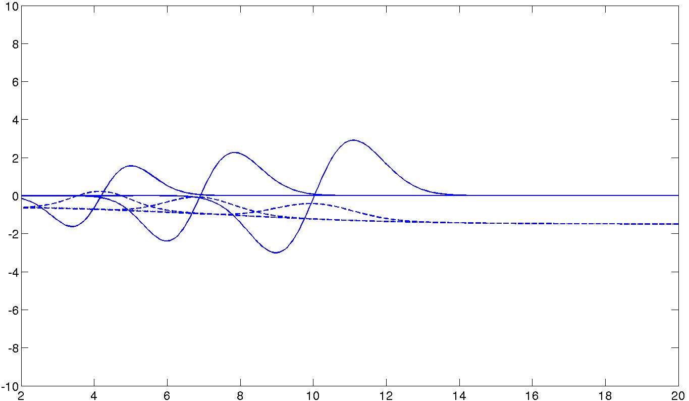
Refer to caption
Figure 2: Evolution of the maximum of ζ1\zeta_{1}, solution of (52), for a non flat bottom b0b_{0}.
Refer to caption
Figure 3: Evolution of the surface ζ1\zeta_{1} (solid line), solution of (52), and the landslide bmb_{m} (dashed line).
Refer to caption
Figure 4: Evolution of the maximum of hh, solution of (52), with non trivial initial data and with bmb_{m} like in Figure 3.

3.3 Linear asymptotic and resonance in intermediate depths

In this case, we consider only that ε\varepsilon, β\beta are small. Physically, this means that we consider small amplitudes for the surface and the bottom (compared to the mean depth) and that the depth is not small compared to wavelength of the waves. In this part, we generalize the Proudman resonance in deeper waters. The asymptotic regime is

𝒜L​W​W={(ε,β,λ,μ), 0<ε, β≤δ0, βλ=ε and 0<μ≤μmax},\mathcal{A}_{LWW}=\left\{(\varepsilon,\beta,\lambda,\mu)\text{, }0<\varepsilon\text{, }\beta\leq\delta_{0}\text{, }\beta\lambda=\varepsilon\text{ and }0<\mu\leq\mu_{\max}\right\}, (55)

with δ0≪1\delta_{0}\ll 1 and 0<μmax0<\mu_{\max}. Using the energy

ℰ⁡(t)=12​|ζ|L22+12​(1μ​Gμ​[0,0]​(ψ),ψ)L2,\mathcal{E}(t)=\frac{1}{2}\left\lvert\zeta\right\rvert_{L^{2}}^{2}+\frac{1}{2}\left(\frac{1}{\mu}G_{\mu}[0,0](\psi),\psi\right)_{L^{2}},

and proceeding as in Proposition 3.4 (we need also Proposition 3.12 in [19]), we get a new asymptotic model.

Proposition 3.9.

Let t0>d2t_{0}\hskip-1.42271pt>\hskip-1.42271pt\frac{d}{2}, N≥max⁡(1,t0)+3N\hskip-1.42271pt\geq\hskip-1.42271pt\max(1,t_{0})+3, b∈W3,∞​(ℝ+,HN​(ℝd))b\in W^{3,\infty}(\mathbb{R}^{+};H^{N}(\mathbb{R}^{d})), U0=(ζ0,ψ0)∈E0NU^{0}\hskip-1.42271pt=\hskip-1.42271pt\left(\zeta_{0},\psi_{0}\right)\in E_{0}^{N} and P∈W1,∞​(ℝ+,H˙N+1​(ℝd))P\hskip-1.42271pt\in\hskip-1.42271ptW^{1,\infty}(\mathbb{R}^{+};\hskip-1.42271pt\dot{H}^{N+1}(\mathbb{R}^{d})). We suppose that (19) and (29) are satisfied initially. Then, there exists T>0T>0, such that for all (ε,β,λ,μ)∈𝒜L​W​W(\varepsilon,\beta,\lambda,\mu)\hskip-2.84544pt\in\hskip-2.84544pt\mathcal{A}_{LWW}, there exists a unique solution U=(ζ,ψ)∈ETδ0NU=(\zeta,\psi)\hskip-1.42271pt\in E^{N}_{\frac{T}{\sqrt{\delta_{0}}}} to the water waves equations with initial data U0U^{0}. Furthermore, for all α∈[0,13)\alpha\in\left[0,\frac{1}{3}\right),

|ζ−ζ~|L∞​([0,Tδ0α],HN−2​(ℝd))+||D|1+|D|​(ψ−ψ~)|L∞​([0,Tδ0α],HN−2​(ℝd))≤T​δ01−3​α​C~,\left\lvert\zeta-\widetilde{\zeta}\right\rvert_{L^{\infty}\left(\left[0,\frac{T}{\delta^{\alpha}_{0}}\right];H^{N-2}(\mathbb{R}^{d})\right)}+\left\lvert\frac{|D|}{\sqrt{1+|D|}}\left(\psi-\widetilde{\psi}\right)\right\rvert_{L^{\infty}\left(\left[0,\frac{T}{\delta^{\alpha}_{0}}\right];H^{N-2}(\mathbb{R}^{d})\right)}\leq T\delta_{0}^{1-3\alpha}\widetilde{C},

where

C~=C⁡(ℰN​(U0),1hmin,1𝔞min,μmax,|b|Wt3,∞​HXN,|∇P|Wt1,∞​HXN),\widetilde{C}=C\left(\mathcal{E}^{N}\left(U^{0}\right),\frac{1}{h_{\min}},\frac{1}{\mathfrak{a}_{\min}},\mu_{\max},|b|_{W^{3,\infty}_{t}H^{N}_{\!X}},\left\lvert\nabla P\right\rvert_{W^{1,\infty}_{t}H^{N}_{\!X}}\right),

where (ζ~,ψ~)\left(\widetilde{\zeta},\widetilde{\psi}\right) is a solution of the waves equation

{∂tζ~−1μ​Gμ​[0,0]​(ψ~)=GμN​N​[0,0]​(∂tb),∂tψ~+ζ~=−P,\left\{\begin{aligned} &\partial_{t}\widetilde{\zeta}-\frac{1}{\mu}G_{\mu}[0,0](\widetilde{\psi})=G_{\mu}^{N\!N}[0,0](\partial_{t}b),\\ &\partial_{t}\widetilde{\psi}+\widetilde{\zeta}=-P,\\ \end{aligned}\right. (56)

with initial data U0U^{0}.

The Proudman resonance is a phenomenon which occurs in shallow water regime. We wonder if there is also a resonance in deeper waters. In this part, we only work with a non constant pressure and hence ∂tb=0\partial_{t}b=0. The same study can be done for a moving bottom. We consider the equation (56) for d=1d=1. Since, the initial data does not affect the possible resonance, we suppose in the following that U0=0U^{0}=0. We transform the system (56) in order to have a unique equation for ζ~\widetilde{\zeta} (in the following we denote ζ~\widetilde{\zeta} by ζ\zeta to simplify the notation)

{∂t2ζ+1μ​Gμ​[0,0]​(ζ)=−1μ​Gμ​[0,0]​(P),ζ|t=0=0, ∂tζ|t=0=0.\left\{\begin{aligned} &\partial_{t}^{2}\zeta+\frac{1}{\mu}G_{\mu}[0,0](\zeta)=-\frac{1}{\mu}G_{\mu}[0,0](P),\\ &\zeta_{|t=0}=0\text{, }\partial_{t}\zeta_{|t=0}=0.\end{aligned}\right.

We can solve explicitly the previous equation, we get that

ζ^​(t,ξ)\displaystyle\widehat{\zeta}(t,\xi) =i2​∫0tξ​tanh⁡(μ​|ξ|)μ​|ξ|​P^​(τ,ξ)​ei⁡(t−τ)​ξ​tanh⁡(μ​|ξ|)μ​|ξ|​dτ⏟:=ζ^L​(t,ξ)\displaystyle=\underbrace{\frac{i}{2}\int_{0}^{t}\xi\sqrt{\frac{\tanh(\sqrt{\mu}|\xi|)}{\sqrt{\mu}|\xi|}}\widehat{P}(\tau,\xi)e^{i(t-\tau)\xi\sqrt{\frac{\tanh(\sqrt{\mu}|\xi|)}{\sqrt{\mu}|\xi|}}}d\tau}_{:=\widehat{\zeta}_{L}(t,\xi)}
−i2​∫0tξ​tanh⁡(μ​|ξ|)μ​|ξ|​P^​(τ,ξ)​ei⁡(τ−t)​ξ​tanh⁡(μ​|ξ|)μ​|ξ|​dτ⏟:=ζ^R​(t,ξ).\displaystyle-\underbrace{\frac{i}{2}\int_{0}^{t}\xi\sqrt{\frac{\tanh(\sqrt{\mu}|\xi|)}{\sqrt{\mu}|\xi|}}\widehat{P}(\tau,\xi)e^{i(\tau-t)\xi\sqrt{\frac{\tanh(\sqrt{\mu}|\xi|)}{\sqrt{\mu}|\xi|}}}d\tau}_{:=\widehat{\zeta}_{R}(t,\xi)}.

In order to find a resonant pressure, we suppose that PP has the form e−i​t​a​(D)​P0e^{-ita(D)}P_{0}, where aa is a real smooth odd function which is sublinear, there exists C>0C>0 such that |a⁡(ξ)|≤C​|ξ||a(\xi)|\leq C|\xi|. We also suppose that the phase velocity of the disturbance is positive, a⁡(ξ)ξ≥0\frac{a(\xi)}{\xi}\geq 0. P0P_{0} is a smooth function in a Sobolev space with P0^​(0)≠0\widehat{P_{0}}(0)\neq 0. We denote ω⁡(ξ)=tanh⁡(ξ)ξ\omega(\xi)=\sqrt{\frac{\tanh(\xi)}{\xi}}. A simple computation gives that

|ζL​(t,⋅)|≤|ζL^​(t,⋅)|L1≤|P0^|L1.|\zeta_{L}(t,\cdot)|\leq|\widehat{\zeta_{L}}(t,\cdot)|_{L^{1}}\leq\left\lvert\widehat{P_{0}}\right\rvert_{L^{1}}.

Furthermore, we have

|ζR^​(t,ξ)|\displaystyle|\widehat{\zeta_{R}}(t,\xi)| =12​|∫0tξ​ω​(μ​ξ)​P^0​(ξ)​ei​τ​(ξ​ω​(μ​ξ)−a⁡(ξ))​𝑑τ|\displaystyle=\frac{1}{2}\left\lvert\int_{0}^{t}\xi\omega(\sqrt{\mu}\xi)\widehat{P}_{0}(\xi)e^{i\tau\left(\xi\omega(\sqrt{\mu}\xi)-a(\xi)\right)}d\tau\right\rvert
≤t2​|ξ​ω​(μ​ξ)​P^0​(ξ)|,\displaystyle\leq\frac{t}{2}\left\lvert\xi\omega(\sqrt{\mu}\xi)\widehat{P}_{0}(\xi)\right\rvert,

with an equality if and only if a⁡(ξ)=ξ​ω​(μ​ξ)a(\xi)=\xi\omega(\sqrt{\mu}\xi). Hence, it is natural to consider that

P^​(t,ξ)=e−i​t​ξ​ω​(μ​ξ)​P0​(ξ).\widehat{P}(t,\xi)=e^{-it\xi\omega(\sqrt{\mu}\xi)}P_{0}(\xi). (57)

A simple computation gives

ζR(t,X)=−i​t2∫ℝξω(μξ)P0^(ξ)e−i​t​ξ​ω​(μ​ξ)ei​X​ξdξ.\zeta_{R}(t,X)=-\frac{it}{2}\int_{\mathbb{R}}\xi\omega(\sqrt{\mu}\xi)\widehat{P_{0}}(\xi)e^{-it\xi\omega(\sqrt{\mu}\xi)}e^{iX\xi}d\xi. (58)

We wonder now if a resonance occurs. We need a dispersion estimate for the linear water waves equation.

Proposition 3.10.

Let f∈W1,1​(ℝ)f\in W^{1,1}(\mathbb{R}) such that f^​(0)=0\widehat{f}(0)=0. Then,

|∫ℝe−i​t​ξ​ω​(μ​ξ)​ei​X​ξ​f^​(ξ)​𝑑ξ|≤Ct​(1μ​|1|ξ|​(f^)′|L1​(ℝ)+μ18​||ξ|34​(f^)′|L1​(ℝ)).\left\lvert\int_{\mathbb{R}}e^{-it\xi\omega(\sqrt{\mu}\xi)}e^{iX\xi}\widehat{f}(\xi)d\xi\right\rvert\leq\frac{C}{\sqrt{t}}\left(\frac{1}{\sqrt{\mu}}\left\lvert\frac{1}{\sqrt{\left\lvert\xi\right\rvert}}\left(\widehat{f}\right)^{\prime}\right\rvert_{L^{1}(\mathbb{R})}+\mu^{\frac{1}{8}}\left\lvert\left\lvert\xi\right\rvert^{\frac{3}{4}}\left(\widehat{f}\right)^{\prime}\right\rvert_{L^{1}(\mathbb{R})}\right).
Proof.

We denote I⁡(t)I(t),

I⁡(t)\displaystyle I(t) :=∫ℝe−i​t​ξ​ω​(μ​ξ)​ei​X​ξ​f^​(ξ)​𝑑ξ\displaystyle:=\int_{\mathbb{R}}e^{-it\xi\omega(\sqrt{\mu}\xi)}e^{iX\xi}\widehat{f}(\xi)d\xi
=1μ​∫ℝe−i​tμ​(y​ω​(y)−Xt​y)​f^​(yμ)​𝑑y.\displaystyle=\frac{1}{\sqrt{\mu}}\int_{\mathbb{R}}e^{-i\frac{t}{\sqrt{\mu}}\left(y\omega(y)-\frac{X}{t}y\right)}\widehat{f}\left(\frac{y}{\sqrt{\mu}}\right)dy.

We denote ϕ\phi,

ϕ⁡(y)=y​ω​(y)−Xt​y,\phi(y)=y\omega(y)-\frac{X}{t}y,

and y0y_{0} the unique minimum of ϕ′′\phi^{\prime\prime}. Figure 5 represents ϕ′′\phi^{\prime\prime} on [0,+∞[[0,+\infty[.

Refer to caption
Figure 5: Profile of ϕ′′\phi^{\prime\prime} .

To estimate I⁡(t)I(t) we decompose I⁡(t)I(t) into four parts.

I1​(t)\displaystyle I_{1}(t) =1μ​∫0y0e−i​tμ​ϕ​(y)​f^​(yμ)​𝑑y\displaystyle=\frac{1}{\sqrt{\mu}}\int_{0}^{y_{0}}e^{-i\frac{t}{\sqrt{\mu}}\phi(y)}\widehat{f}\left(\frac{y}{\sqrt{\mu}}\right)dy
=1μ∫0y0−dd​y(∫yy0e−i​tμ​ϕ​(z)dz)f^(yμ)dy\displaystyle=\frac{1}{\sqrt{\mu}}\int_{0}^{y_{0}}-\frac{d}{dy}\left(\int_{y}^{y_{0}}e^{-i\frac{t}{\sqrt{\mu}}\phi(z)}dz\right)\widehat{f}\left(\frac{y}{\sqrt{\mu}}\right)dy
=1μ​∫0y0∫yy0e−i​tμ​ϕ​(z)​𝑑z​(f^)′​(yμ)​𝑑y.\displaystyle=\frac{1}{\mu}\int_{0}^{y_{0}}\int_{y}^{y_{0}}e^{-i\frac{t}{\sqrt{\mu}}\phi(z)}dz\left(\widehat{f}\right)^{\prime}\left(\frac{y}{\sqrt{\mu}}\right)dy.

Then, using Van der Corput’s Lemma (see [26]) and the fact that for z∈[y,y0]z\in[y,y_{0}],
|ϕ′′​(z)|≥|ϕ′′​(y)||\phi^{\prime\prime}(z)|\geq|\phi^{\prime\prime}(y)| and |ϕ′′​(z)|≥C​z|\phi^{\prime\prime}(z)|\geq Cz,

|I1​(t)|\displaystyle|I_{1}(t)| ≤Cμ34​t​∫0y0|1y​(f^)′​(yμ)|​𝑑y\displaystyle\leq\frac{C}{\mu^{\frac{3}{4}}\sqrt{t}}\int_{0}^{y_{0}}\left\lvert\frac{1}{\sqrt{y}}\left(\widehat{f}\right)^{\prime}\left(\frac{y}{\sqrt{\mu}}\right)\right\rvert dy
≤Cμ​t​∫0+∞|1ξ​(f^)′​(ξ)|​𝑑ξ.\displaystyle\leq\frac{C}{\sqrt{\mu}\sqrt{t}}\int_{0}^{+\infty}\left\lvert\frac{1}{\sqrt{\xi}}\left(\widehat{f}\right)^{\prime}\left(\xi\right)\right\rvert d\xi.

Furthermore, for M>y0M>y_{0} large enough,

I2​(t)\displaystyle I_{2}(t) =1μ​∫y0Me−i​tμ​ϕ​(y)​f^​(yμ)​𝑑y\displaystyle=\frac{1}{\sqrt{\mu}}\int_{y_{0}}^{M}e^{-i\frac{t}{\sqrt{\mu}}\phi(y)}\widehat{f}\left(\frac{y}{\sqrt{\mu}}\right)dy
=1μ​∫y0Mdd​y​(∫y0ye−i​tμ​ϕ​(z)​𝑑z)​f^​(yμ)​𝑑y\displaystyle=\frac{1}{\sqrt{\mu}}\int_{y_{0}}^{M}\frac{d}{dy}\left(\int_{y_{0}}^{y}e^{-i\frac{t}{\sqrt{\mu}}\phi(z)}dz\right)\widehat{f}\left(\frac{y}{\sqrt{\mu}}\right)dy
=∫y0Me−i​tμ​ϕ​(z)​d​zμ​f^​(Mμ)−1μ​∫y0M∫y0ye−i​tμ​ϕ​(z)​𝑑z​(f^)′​(yμ)​𝑑y.\displaystyle=\int_{y_{0}}^{M}\hskip-2.84544pte^{-i\frac{t}{\sqrt{\mu}}\phi(z)}\frac{dz}{\sqrt{\mu}}\widehat{f}\left(\frac{M}{\sqrt{\mu}}\right)-\frac{1}{\mu}\int_{y_{0}}^{M}\int_{y_{0}}^{y}e^{-i\frac{t}{\sqrt{\mu}}\phi(z)}dz\left(\widehat{f}\right)^{\prime}\left(\frac{y}{\sqrt{\mu}}\right)dy.

Then, ​ using Van der Corput’s Lemma and the fact that for z∈[y0,y]z\in[y_{0},y],
|ϕ′′​(z)|≥|ϕ′′​(y)||\phi^{\prime\prime}(z)|\geq|\phi^{\prime\prime}(y)| and |ϕ′′​(z)|≥C​z−32|\phi^{\prime\prime}(z)|\geq Cz^{-\frac{3}{2}},

|I2​(t)|\displaystyle|I_{2}(t)| ≤|Mμ​f^​(Mμ)|+Cμ34​t​∫y0M|y34​(f^)′​(yμ)|​𝑑y\displaystyle\leq\left\lvert\frac{M}{\sqrt{\mu}}\widehat{f}\left(\frac{M}{\sqrt{\mu}}\right)\right\rvert+\frac{C}{\mu^{\frac{3}{4}}\sqrt{t}}\int_{y_{0}}^{M}\left\lvert y^{\frac{3}{4}}\left(\widehat{f}\right)^{\prime}\left(\frac{y}{\sqrt{\mu}}\right)\right\rvert dy
≤|f′^​(Mμ)|+C​μ18t​∫0+∞|ξ34​(f^)′​(ξ)|.\displaystyle\leq\left\lvert\widehat{f^{\prime}}\left(\frac{M}{\sqrt{\mu}}\right)\right\rvert+\frac{C\mu^{\frac{1}{8}}}{\sqrt{t}}\int_{0}^{+\infty}\left\lvert\xi^{\frac{3}{4}}\left(\widehat{f}\right)^{\prime}\left(\xi\right)\right\rvert.

Tending MM to +∞+\infty we get the result. The control for ξ<0\xi<0 is similar. ∎

Therefore, in the linear case, we have also a resonance.

Corollary 3.11.

Let P0∈H3​(ℝ)∩W2,1​(ℝ)P_{0}\in H^{3}(\mathbb{R})\cap W^{2,1}(\mathbb{R}) such that X​P0∈H3​(ℝ)XP_{0}\in H^{3}(\mathbb{R}) and let
0<μ≤μmax0<\mu\leq\mu_{\max}. Consider,

ζR(t,X)=−i​t2∫ℝξω(μξ)P0^(ξ)e−i​t​ξ​ω​(μ​ξ)ei​X​ξdξ.\zeta_{R}(t,X)=-\frac{it}{2}\int_{\mathbb{R}}\xi\omega(\sqrt{\mu}\xi)\widehat{P_{0}}(\xi)e^{-it\xi\omega(\sqrt{\mu}\xi)}e^{iX\xi}d\xi.

Then,

|ζR​(t,⋅)|∞≤C⁡(μmax)​tμ​(|P0|H3+|P0|L1+|X​P0|H3),\left\lvert\zeta_{R}(t,\cdot)\right\rvert_{\infty}\leq C(\mu_{\max})\sqrt{\frac{t}{\mu}}\left(\left\lvert P_{0}\right\rvert_{H^{3}}+\left\lvert P_{0}\right\rvert_{L^{1}}+\left\lvert XP_{0}\right\rvert_{H^{3}}\right),

and

lim¯t→+∞​|1t​ζR​(t,⋅)|∞≥C⁡(P0)>0.\underset{t\shortrightarrow+\infty}{\underline{\lim}}\left\lvert\frac{1}{\sqrt{t}}\zeta_{R}(t,\cdot)\right\rvert_{\infty}\geq C(P_{0})>0.
Proof.

We take f^​(ξ)=ξ​ω​(μ​ξ)​P^0​(ξ)\widehat{f}(\xi)=\xi\omega(\sqrt{\mu}\xi)\widehat{P}_{0}(\xi). Then,

|(f^)′​(ξ)|≤(1+μ​|ξ|)​|P^0​(ξ)|+|ξ|​|(P^0)′​(ξ)|,\left\lvert\left(\widehat{f}\right)^{\prime}\hskip-5.69046pt(\xi)\right\rvert\leq\left(1+\sqrt{\mu}|\xi|\right)\left\lvert\widehat{P}_{0}(\xi)\right\rvert+|\xi|\left\lvert\left(\widehat{P}_{0}\right)^{\prime}\hskip-5.69046pt(\xi)\right\rvert,

and the first inequality follows from the previous Proposition. For the second inequality, we use a stationary phase approximation. We denote ϕ⁡(ξ)=ξ​ω​(ξ)\phi(\xi)=\xi\omega(\xi). Let ξ0>0\xi_{0}>0, such that |ξ0​P0^​(ξ0)|=|ξ​P0^|L∞\left\lvert\xi_{0}\widehat{P_{0}}(\xi_{0})\right\rvert=\left\lvert\xi\widehat{P_{0}}\right\rvert_{L^{\infty}}, and Xμ<0X_{\mu}<0, such that ϕ′​(μ​ξ0)=Xμ\phi^{\prime}(\sqrt{\mu}\xi_{0})=X_{\mu}. Then, we have,

limt→+∞​|1t​ζR​(t,t​Xμ)|\displaystyle\underset{t\shortrightarrow+\infty}{\lim}\left\lvert\frac{1}{\sqrt{t}}\zeta_{R}(t,tX_{\mu})\right\rvert =limt→+∞​t2​μ​|∫ℝξ​ω​(ξ)​P0^​(ξμ)​e−i​tμ​ξ​(ω⁡(ξ)−Xμ)​𝑑ξ|\displaystyle=\underset{t\shortrightarrow+\infty}{\lim}\frac{\sqrt{t}}{2\mu}\left\lvert\int_{\mathbb{R}}\xi\omega(\xi)\widehat{P_{0}}\left(\frac{\xi}{\sqrt{\mu}}\right)e^{-i\frac{t}{\sqrt{\mu}}\xi\left(\omega(\xi)-X_{\mu}\right)}d\xi\right\rvert
=2​π2​μ14​|ω⁡(ξ0​μ)​ξ0​P0^​(ξ0)|ϕ′′​(ξ0​μ)||.\displaystyle=\frac{\sqrt{2\pi}}{2\mu^{\frac{1}{4}}}\left\lvert\frac{\omega(\xi_{0}\sqrt{\mu})\xi_{0}\widehat{P_{0}}(\xi_{0})}{\sqrt{|\phi^{\prime\prime}(\xi_{0}\sqrt{\mu})|}}\right\rvert.

Since |ϕ′′​(ξ)|≤C​|ξ||\phi^{\prime\prime}(\xi)|\leq C|\xi| and ω⁡(ξ0​μ)≥C⁡(ξ0)​μ\omega(\xi_{0}\sqrt{\mu})\geq C(\xi_{0})\sqrt{\mu}, we get the result.

∎

Remark 3.12.

Notice that for all s∈ℝs\in\mathbb{R},

|ζR(t,⋅)+t2P0′(⋅−t)|Hs≤μt2|∇P0|Hs+2.\left\lvert\zeta_{R}(t,\cdot)+\frac{t}{2}P_{0}^{\prime}(\cdot-t)\right\rvert_{H^{s}}\leq\sqrt{\mu}t^{2}\left\lvert\nabla P_{0}\right\rvert_{H^{s+2}}.

Hence, by tending formally μ\mu to 00, we rediscover the result we get in the shallow water case (section 3.1).

Remark 3.13.

Notice that for a general pressure term P⁡(t,X)P(t,X) we can show that the amplitude ζ\zeta satisfying

ζ^​(t,ξ)\displaystyle\widehat{\zeta}(t,\xi) =i2​∫0tξ​tanh⁡(μ​|ξ|)μ​|ξ|​P^​(τ,ξ)​ei⁡(t−τ)​ξ​tanh⁡(μ​|ξ|)μ​|ξ|​𝑑τ\displaystyle=\frac{i}{2}\int_{0}^{t}\xi\sqrt{\frac{\tanh(\sqrt{\mu}|\xi|)}{\sqrt{\mu}|\xi|}}\widehat{P}(\tau,\xi)e^{i(t-\tau)\xi\sqrt{\frac{\tanh(\sqrt{\mu}|\xi|)}{\sqrt{\mu}|\xi|}}}d\tau
−i2∫0tξtanh⁡(μ​|ξ|)μ​|ξ|P^(τ,ξ)ei⁡(τ−t)​ξ​tanh⁡(μ​|ξ|)μ​|ξ|dτ,\displaystyle-\frac{i}{2}\int_{0}^{t}\xi\sqrt{\frac{\tanh(\sqrt{\mu}|\xi|)}{\sqrt{\mu}|\xi|}}\widehat{P}(\tau,\xi)e^{i(\tau-t)\xi\sqrt{\frac{\tanh(\sqrt{\mu}|\xi|)}{\sqrt{\mu}|\xi|}}}d\tau,

satisfies also

|ζ⁡(t,⋅)|∞≤C⁡(μmax)​tμ​(|P|L∞​(ℝ+,L1​(ℝd))+|P|L∞​(ℝ+;H3​(ℝd)CLOSE+|X​P|L∞​(ℝ+;H3​(ℝd)CLOSE).\left\lvert\zeta(t,\cdot)\right\rvert_{\infty}\leq C(\mu_{\max})\sqrt{\frac{t}{\mu}}\left(\left\lvert P\right\rvert_{L^{\infty}(\mathbb{R}^{+};L^{1}(\mathbb{R}^{d}))}+\left\lvert P\right\rvert_{L^{\infty}(\mathbb{R}^{+};H^{3}(\mathbb{R}^{d})}+\left\lvert XP\right\rvert_{L^{\infty}(\mathbb{R}^{+};H^{3}(\mathbb{R}^{d})}\right).

Hence, contrary to the shallow water case, we can not hope a linear amplification with respect to the time tt. Corollary 3.11 also shows that the factor of amplification of t\sqrt{t} is optimal.

Hence, we observe that in intermediate water depths, a resonance can occur but with a factor of amplification of t\sqrt{t} and not tt. But we saw that in the shallow water case, the resonance occurs for a moving pressure with a speed equal to 11, P⁡(t,X)=P0​(X−t)P(t,X)=P_{0}(X-t). We wonder if this pressure can create a resonance. The following Proposition shows that the previous pressure can create a resonance with a factor of amplification of t13t^{\frac{1}{3}}.

Proposition 3.14.

Let 0<μ≤μmax0<\mu\leq\mu_{\max}. Let P0∈L1​(ℝ)∩H1​(ℝ)P_{0}\in L^{1}(\mathbb{R})\cap H^{1}(\mathbb{R}) such that P0^​(0)≠0\widehat{P_{0}}(0)\neq 0. Consider, the amplitude ζR\zeta_{R} created by P⁡(t,X)=P0​(X−t)P(t,X)=P_{0}(X-t),

ζR^(t,ξ)=−i2ξω(μξ)P0^(ξ)e−i​t​ξ∫−t0ei​s​ξ​(ω⁡(μ​ξ)−1)ds.\widehat{\zeta_{R}}(t,\xi)=-\frac{i}{2}\xi\omega(\sqrt{\mu}\xi)\widehat{P_{0}}(\xi)e^{-it\xi}\int_{-t}^{0}e^{is\xi\left(\omega(\sqrt{\mu}\xi)-1\right)}ds. (59)

Then,

|ζR​(t,⋅)|∞≤C⁡(μmax)​(t13μ​|P0|L1+μ14​|P0|H1).\left\lvert\zeta_{R}(t,\cdot)\right\rvert_{\infty}\leq C(\mu_{\max})\left(\frac{t^{\frac{1}{3}}}{\mu}\left\lvert P_{0}\right\rvert_{L^{1}}+\mu^{\frac{1}{4}}\left\lvert P_{0}\right\rvert_{H^{1}}\right).

Furthermore, if X​P0∈H1​(ℝ)XP_{0}\in H^{1}(\mathbb{R}),

lim¯t→+∞​|1t13​ζR​(t,⋅)|∞≥Cμ23​|P0^​(0)|.\underset{t\shortrightarrow+\infty}{\underline{\lim}}\left\lvert\frac{1}{t^{\frac{1}{3}}}\zeta_{R}(t,\cdot)\right\rvert_{\infty}\geq\frac{C}{\mu^{\frac{2}{3}}}\left\lvert\widehat{P_{0}}(0)\right\rvert.
Proof.

We have

ζR​(t,X)\displaystyle\zeta_{R}(t,X) =−i2∫ℝξω(μξ)P0^(ξ)e−i​t​ξ∫−t0ei​s​ξ​(ω⁡(μ​ξ)−1)ei​X​ξdsdξ\displaystyle=-\frac{i}{2}\int_{\mathbb{R}}\xi\omega(\sqrt{\mu}\xi)\widehat{P_{0}}(\xi)e^{-it\xi}\int_{-t}^{0}e^{is\xi\left(\omega(\sqrt{\mu}\xi)-1\right)}e^{iX\xi}dsd\xi
=−i21μ∫ℝξω(ξ)P0^(ξμ)e−i​tμ​ξ∫−t0ei​sμ​ξ​(ω⁡(ξ)−1)ei​Xμ​ξdsdξ.\displaystyle=-\frac{i}{2}\frac{1}{\mu}\int_{\mathbb{R}}\xi\omega(\xi)\widehat{P_{0}}\left(\frac{\xi}{\sqrt{\mu}}\right)e^{-i\frac{t}{\sqrt{\mu}}\xi}\int_{-t}^{0}e^{i\frac{s}{\sqrt{\mu}}\xi\left(\omega(\xi)-1\right)}e^{i\frac{X}{\sqrt{\mu}}\xi}dsd\xi.

We decompose this integral into 33 parts.

|I1​(t)|\displaystyle\left\lvert I_{1}(t)\right\rvert =|1μ​∫|ξ|≤t−13ξ​ω​(ξ)​P0^​(ξμ)​e−i​tμ​ξ​∫−t0ei​sμ​ξ​(ω⁡(ξ)−1)​ei​Xμ​ξ​𝑑ξ​𝑑s|\displaystyle=\left\lvert\frac{1}{\mu}\int_{|\xi|\leq t^{-\frac{1}{3}}}\xi\omega(\xi)\widehat{P_{0}}\left(\frac{\xi}{\sqrt{\mu}}\right)e^{-i\frac{t}{\sqrt{\mu}}\xi}\int_{-t}^{0}e^{i\frac{s}{\sqrt{\mu}}\xi\left(\omega(\xi)-1\right)}e^{i\frac{X}{\sqrt{\mu}}\xi}d\xi ds\right\rvert
≤t13μ​|P0^|∞.\displaystyle\leq\frac{t^{\frac{1}{3}}}{\mu}\left\lvert\widehat{P_{0}}\right\rvert_{\infty}.

Furthermore, since |ω⁡(ξ)−1|≥C​ξ2\left\lvert\omega(\xi)-1\right\rvert\geq C\xi^{2} for 0≤|ξ|≤10\leq|\xi|\leq 1, we have

|I2​(t)|\displaystyle\left\lvert I_{2}(t)\right\rvert =|1μ​∫t−13≤|ξ|≤1ξ​ω​(ξ)​P0^​(ξμ)​e−i​tμ​ξ​∫−t0ei​sμ​ξ​(ω⁡(ξ)−1)​ei​Xμ​ξ​𝑑ξ​𝑑s|\displaystyle=\left\lvert\frac{1}{\mu}\int_{t^{-\frac{1}{3}}\leq|\xi|\leq 1}\xi\omega(\xi)\widehat{P_{0}}\left(\frac{\xi}{\sqrt{\mu}}\right)e^{-i\frac{t}{\sqrt{\mu}}\xi}\int_{-t}^{0}e^{i\frac{s}{\sqrt{\mu}}\xi\left(\omega(\xi)-1\right)}e^{i\frac{X}{\sqrt{\mu}}\xi}d\xi ds\right\rvert
=|1μ​∫t−13≤|ξ|≤1ei​Xμ​ξ​ω⁡(ξ)ω⁡(ξ)−1​P0^​(ξμ)​(e−i​tμ​ξ−e−i​tμ​ξ​ω​(ξ))​𝑑ξ|\displaystyle=\left\lvert\frac{1}{\sqrt{\mu}}\int_{t^{-\frac{1}{3}}\leq|\xi|\leq 1}e^{i\frac{X}{\sqrt{\mu}}\xi}\frac{\omega(\xi)}{\omega(\xi)-1}\widehat{P_{0}}\left(\frac{\xi}{\sqrt{\mu}}\right)\left(e^{-i\frac{t}{\sqrt{\mu}}\xi}-e^{-i\frac{t}{\sqrt{\mu}}\xi\omega(\xi)}\right)d\xi\right\rvert
≤C​t13μ​|P0^|∞.\displaystyle\leq C\frac{t^{\frac{1}{3}}}{\sqrt{\mu}}\left\lvert\widehat{P_{0}}\right\rvert_{\infty}.

Finally,

|I3​(t)|\displaystyle\left\lvert I_{3}(t)\right\rvert =|1μ​∫|ξ|≥1ξ​ω​(ξ)​P0^​(ξμ)​e−i​tμ​ξ​∫−t0ei​sμ​ξ​(ω⁡(μ​ξ)−1)​ei​Xμ​ξ​𝑑ξ​𝑑s|\displaystyle=\left\lvert\frac{1}{\mu}\int_{|\xi|\geq 1}\xi\omega(\xi)\widehat{P_{0}}\left(\frac{\xi}{\sqrt{\mu}}\right)e^{-i\frac{t}{\sqrt{\mu}}\xi}\int_{-t}^{0}e^{i\frac{s}{\sqrt{\mu}}\xi\left(\omega(\sqrt{\mu}\xi)-1\right)}e^{i\frac{X}{\sqrt{\mu}}\xi}d\xi ds\right\rvert
=|1μ​∫|ξ|≥1ei​Xμ​ξ​ω⁡(ξ)ω⁡(ξ)−1​P0^​(ξμ)​(e−i​tμ​ξ−e−i​tμ​ξ​ω​(ξ))​𝑑ξ|\displaystyle=\left\lvert\frac{1}{\sqrt{\mu}}\int_{|\xi|\geq 1}e^{i\frac{X}{\sqrt{\mu}}\xi}\frac{\omega(\xi)}{\omega(\xi)-1}\widehat{P_{0}}\left(\frac{\xi}{\sqrt{\mu}}\right)\left(e^{-i\frac{t}{\sqrt{\mu}}\xi}-e^{-i\frac{t}{\sqrt{\mu}}\xi\omega(\xi)}\right)d\xi\right\rvert
≤C​∫|ξ|≥1μ|P0^​(ξ)|​𝑑ξ,\displaystyle\leq C\int_{|\xi|\geq\frac{1}{\sqrt{\mu}}}\left\lvert\widehat{P_{0}}(\xi)\right\rvert d\xi,
≤C​μ14​|P0|H1,\displaystyle\leq C\mu^{\frac{1}{4}}\left\lvert P_{0}\right\rvert_{H^{1}},

and the first inequality follows. For the second inequality, we use a stationary phase approximation. We denote ϕ⁡(ξ):=ξ⁡(ω⁡(ξ)−1)\phi(\xi):=\xi(\omega(\xi)-1). We recall that ϕ⁡(ξ)=−16​ξ3+o⁡(ξ3)\phi(\xi)=-\frac{1}{6}\xi^{3}+o(\xi^{3}). Using a generalization of Morse Lemma at the order 33, there exists a>0a>0 and ψ∈𝒞∞​([−a,a])\psi\in\mathcal{C}^{\infty}\left([-a,a]\right), such that for all |y|≤a|y|\leq a,

ϕ⁡(ψ⁡(y))=16​ϕ′′′​(0)​y3,ψ⁡(0)=0​ and ​ψ′​(0)=1.\phi(\psi(y))=\frac{1}{6}\phi^{\prime\prime\prime}(0)y^{3},\psi(0)=0\text{ and }\psi^{\prime}(0)=1.

Then,

I⁡(s)\displaystyle I(s) :=∫ℝω⁡(ξ)​ξ​P0^​(ξμ)​ei​sμ​ξ​(ω⁡(ξ)−1)​𝑑ξ\displaystyle:=\int_{\mathbb{R}}\omega(\xi)\xi\widehat{P_{0}}\left(\frac{\xi}{\sqrt{\mu}}\right)e^{i\frac{s}{\sqrt{\mu}}\xi(\omega(\xi)-1)}d\xi
=∫−aaψ′​(y)​ω​(ψ⁡(y))​ψ​(y)​P0^​(ψ⁡(y)μ)​ei​s6​μ​y3​𝑑y+o⁡(s−23)\displaystyle=\int_{-a}^{a}\psi^{\prime}(y)\omega(\psi(y))\psi(y)\widehat{P_{0}}\left(\frac{\psi(y)}{\sqrt{\mu}}\right)e^{i\frac{s}{6\sqrt{\mu}}y^{3}}dy+o(s^{-\frac{2}{3}})
=(6​μs)23​P0^​(0)​∫z∈ℝz​ei​z3​𝑑z+o⁡(s−23).\displaystyle=\left(\frac{6\sqrt{\mu}}{s}\right)^{\frac{2}{3}}\widehat{P_{0}}(0)\int_{z\in\mathbb{R}}ze^{iz^{3}}dz+o(s^{-\frac{2}{3}}).

Therefore,

limt→+∞​|1t13​ζR​(t,t)|=Cμ23​|P0^​(0)|.\underset{t\shortrightarrow+\infty}{\lim}\left\lvert\frac{1}{t^{\frac{1}{3}}}\zeta_{R}(t,t)\right\rvert=\frac{C}{\mu^{\frac{2}{3}}}\left\lvert\widehat{P_{0}}(0)\right\rvert.

∎

Then, in intermediate water depths, a traveling pressure with a constant speed equal to 11 is also resonant, but it takes more time to obtain a significant elevation of the level of the sea. In the following, we compute numerically some solutions. We take P0​(X)=−e−X2P_{0}(X)=-e^{-X^{2}} and μ=1\mu=1. The figure 6 is the evolution of a water wave because of a pressure of the form (57). The solid curve is the wave and the dashed curve is the moving pressure. The figure 7 is the evolution is a water wave when the pressure moves with a speed 11. The figure 8 compares the evolution of the maximum of the resonant case and the case when the speed is equal to 11.

Refer to caption
Figure 6: Evolution of the surface elevation ζR\zeta_{R} in (58) (solid line) because of a resonant moving pressure PP in (57) (dashed line).
Refer to caption
Figure 7: Evolution of the surface elevation ζR\zeta_{R} in (59) (solid line) because of a moving pressure PP with a speed of 11 (dashed line).
Refer to caption
Figure 8: Evolution of the maximum of ζR\zeta_{R} in the resonant case (solid line) and the moving pressure with a speed of 11 (dashed line).
Remark 3.15.

In our work, we neglect the Coriolis effect. However, in view of the duration of the meteotsunami phenomenon, it would be more realistic to consider it. It will be studied in a future work ([22]) based on the work of A. Castro and D. Lannes ([8] and [9]).

Appendix A The Laplace problem

A.1 Formulation of the problems

In this part, we recall some results of Chapter 2 in [19] and Section 4 of [16] and study the Laplace problem (17) in the Beppo Levi spaces. We suppose that the parameters ε\varepsilon, μ\mu and β\beta satisfy Condition (18). The Laplace problem (17) is

{ΔX,zμ​ΦB=0​ in ​Ωt​ ,ΦB|z=εζ=0 , 1+β2​|∇b|2∂nΦB|z=−1+βb=B,\left\{\begin{aligned} &\Delta^{\mu}_{\!X,z}\Phi^{B}=0\text{ in }\Omega_{t}\text{ ,}\\ &\Phi^{B}_{\;\;\,|z=\varepsilon\zeta}=0\text{ , }\sqrt{1+\beta^{2}|\nabla b|^{2}}\partial_{\textbf{n}}\Phi^{B}_{\;\;\,|z=-1+\beta b}=B,\end{aligned}\right.

where B=∂tbB=\partial_{t}b. Notice that ∂n\partial_{\textbf{n}} is here the upward conormal derivative

∂nΦB=n⋅(μ​Id​00​1)∇μX,zΦB|z=−1+βb.\partial_{\textbf{n}}\Phi^{B}=\textbf{n}\cdot\begin{pmatrix}\sqrt{\mu}I_{d}\hskip 2.84544pt0\\ \hskip 14.22636pt0\hskip 8.5359pt1\end{pmatrix}\nabla^{\mu}_{\!X,z}\Phi^{B}_{\;\;\,|z=-1+\beta b}.

For the study of (15) we refer to [19]. We work with Beppo Levi spaces. We refer to [13] and Proposition 2.3 in [19] for general results about these spaces. We recall that, for s≥0s\geq 0,

H˙s(ℝd):={ψ∈Lloc2(ℝd), ∇ψ∈Hs−1(ℝd)},\dot{H}^{s}(\mathbb{R}^{d}):=\left\{\psi\in L^{2}_{\rm loc}(\mathbb{R}^{d})\text{, }\nabla\psi\in H^{s-1}(\mathbb{R}^{d})\right\},

that H˙1​(ℝd×(−1,0))/ℝ\dot{H}^{1}(\mathbb{R}^{d}\times(-1,0))/\raisebox{-2.79857pt}{$\mathbb{R}$} is a Hilbert space for the norm |∇X,z⋅|L2|\nabla_{\!X,z}\cdot|_{L^{2}} and that Hs​(ℝd)H^{s}(\mathbb{R}^{d}) is dense in H˙s​(ℝd)\dot{H}^{s}(\mathbb{R}^{d}). In order to fix the domain, we transform the problem into variable coefficients elliptic problem on S:=ℝd×(−1,0)S:=\mathbb{R}^{d}\times(-1,0) (the flat strip). We introduce a regularizing diffeomorphism. Let θ:ℝ→ℝ\theta:\mathbb{R}\shortrightarrow\mathbb{R} be a positive, compactly supported, smooth, even function equal to one near 00. For δ>0\delta>0 we define

Σ:=S⟶Ω(X,z)↦(X,z+σ⁡(X,z)),\Sigma:=\begin{array}[]{l}\quad S\quad\longrightarrow\quad\quad\quad\quad\Omega\\ (X,z)\mapsto\left(X,z+\sigma(X,z)\right),\end{array}

and

σ⁡(X,z):=[θ⁡(δ​z​|D|)​ε​ζ​(X)−θ⁡(δ⁡(z+1)​|D|)​β​b​(X)]​z+ε​θ​(δ​z​|D|)​ζ​(X).\sigma(X,z):=\left[\theta(\delta z|D|)\varepsilon\zeta(X)-\theta(\delta(z+1)|D|)\beta b(X)\right]z+\varepsilon\theta(\delta z|D|)\zeta(X).

We omit the dependence on tt here. In the following, we denote by MM a constant of the form

M=C⁡(1hmin,μmax,ε​|ζ|Ht0+1​(ℝd),β​|b|Ht0+1​(ℝd)).M=C\left(\frac{1}{h_{\min}},\mu_{\max},\varepsilon|\zeta|_{H^{t_{0}+1}(\mathbb{R}^{d})},\beta|b|_{H^{t_{0}+1}(\mathbb{R}^{d})}\right).

In order to study the Laplace problems in SS, we have to treat the regularity in the direction XX and in the direction zz one at a time. We introduce the following spaces.

Definition A.1.

Let s∈ℝs\in\mathbb{R}. We define (Hs,1​(S),|⋅|s,1)\left(H^{s,1}(S),\lvert\cdot\rvert_{s,1}\right) and (Hs,0​(S),|⋅|0,1)\left(H^{s,0}(S),\lvert\cdot\rvert_{0,1}\right)

Hs,1​(S):=Lz2​HXs​(S)∩Hz1​HXs−1​(S)​, and ​|u|Hs,12=|Λs​u|L22+|Λs−1​∂zu|L22,H^{s,1}(S):=L^{2}_{z}H^{s}_{X}(S)\cap H^{1}_{z}H^{s-1}_{X}(S)\text{, and }\lvert u\rvert_{H^{s,1}}^{2}=\lvert\Lambda^{s}u\rvert_{L^{2}}^{2}+\lvert\Lambda^{s-1}\partial_{z}u\rvert_{L^{2}}^{2},

and

Hs,0​(S):=Lz2​HXs​(S)​, and ​|u|Hs,02=|Λs​u|L22.H^{s,0}(S):=L^{2}_{z}H^{s}_{X}(S)\text{, and }\lvert u\rvert_{H^{s,0}}^{2}=\lvert\Lambda^{s}u\rvert_{L^{2}}^{2}.
Remark A.2.

We have the following embedding (see Proposition 2.10 in [19]) for s∈ℝs\in\mathbb{R}

Hs+12,1​(S)⊂Lz∞​HXs​(S).H^{s+\frac{1}{2},1}(S)\subset L^{\infty}_{z}H^{s}_{\!X}(S).

In the following, we fix δ>0\delta>0 small enough. Then, we can transform our equations. We denote ϕB:=ΦB∘Σ\phi^{B}:=\Phi^{B}\!\circ\!\Sigma and we get that

{∇X,zμ⋅P⁡(Σ)​∇X,zμϕB=0​ in ​S​,ϕB|z=0=0 , ∂nϕB|z=−1=B,\left\{\begin{aligned} &\nabla^{\mu}_{\!X,z}\cdot P(\Sigma)\nabla^{\mu}_{\!X,z}\phi^{B}=0\text{ in }S\text{,}\\ &\phi^{B}_{\;\,|z=0}=0\text{ , }\partial_{\textbf{n}}\phi^{B}_{\;\,|z=-1}=B,\end{aligned}\right. (60)

with P⁡(Σ)=Id+1×d+1+Q⁡(Σ)P(\Sigma)=I_{d+1\times d+1}+Q(\Sigma) and

Q⁡(Σ):=(∂zσ​Id×d−μ​∇X​σ−μ​∇X​σt−∂zσ+μ|∇Xσ|21+∂zσ).Q(\Sigma):=\begin{pmatrix}\partial_{z}\sigma I_{d\times d}&-\sqrt{\mu}\nabla_{\!X}\sigma\\ -\sqrt{\mu}\nabla_{\!X}\sigma^{t}&\frac{-\partial_{z}\sigma+\mu\left\lvert\nabla_{\!X}\sigma\right\lvert^{2}}{1+\partial_{z}\sigma}\end{pmatrix}. (61)

Notice that P⁡(Σ)P(\Sigma) is well defined if δ\delta is small enough and that ∂n:=ez⋅(P(Σ)∇X,zμ⋅)\partial_{\textbf{n}}:=\textbf{e}_{z}\cdot(P(\Sigma)\nabla^{\mu}_{\!X,z}\;\cdot\;). We have to know the regularity of P⁡(Σ)P(\Sigma). It is the subject of the next proposition (see Proposition 2.18 and Lemma 2.26 in [19]).

Proposition A.3.

Let t0>d2t_{0}>\frac{d}{2}, ζ,b∈Ht0+1​(ℝd)\zeta,b\in H^{t_{0}+1}(\mathbb{R}^{d}) such that Condition (19) is satisfied. Then,

|Q(Σ)|Ht0+12,1,|Λt0Q(Σ)|Lz∞​LX2​(S),|Λt0−1∂zQ(Σ)|Lz∞​LX2​(S)≤M.\left\lvert Q(\Sigma)\right\lvert_{H^{t_{0}+\frac{1}{2},1}}\text{,}\left\lvert\Lambda^{t_{0}}Q(\Sigma)\right\lvert_{L^{\infty}_{z}L^{2}_{X}(S)}\text{,}\left\lvert\Lambda^{t_{0}-1}\partial_{z}Q(\Sigma)\right\lvert_{L^{\infty}_{z}L^{2}_{X}(S)}\leq M.

Furthermore, P⁡(Σ)P(\Sigma) is coercive. There exist a constant k⁡(Σ)>0k(\Sigma)>0 such that 1k⁡(Σ)≤M\frac{1}{k(\Sigma)}\leq M and

∀Θ∈ℝd+1​ , ​∀(X,z)∈S​ , ​P​(Σ)​(X,z)​Θ⋅Θ≥k⁡(Σ)​|Θ|2.\forall\Theta\in\mathbb{R}^{d+1}\text{ , }\forall(X,z)\in S\text{ , }P(\Sigma)(X,z)\Theta\cdot\Theta\geq k(\Sigma)|\Theta|^{2}.

We have a variational formulation of the Laplace problem (60). We introduce

H0,s​u​r​f1(S):=𝒟(S∪{z=−1})¯||H1​(S)=𝒟(S∪{z=−1})¯||H˙1​(S).H^{1}_{0,surf}(S):=\overline{\mathcal{D}(S\cup\{z=-1\})}^{\;|\;|_{H^{1}(S)}}=\overline{\mathcal{D}(S\cup\{z=-1\})}^{\;|\;|_{\dot{H}^{1}(S)}}.

See Proposition 2.3 (3) in [19] for a proof of the second equality.

Definition A.4.

Let B∈H−12​(ℝd)B\in H^{-\frac{1}{2}}(\mathbb{R}^{d}). We say that ϕ∈H0,s​u​r​f1​(S)\phi\in H^{1}_{0,surf}(S) is a variational solution of (60) if for all φ∈H0,s​u​r​f1​(S)\varphi\in H^{1}_{0,surf}(S),

∫S∇X,zμϕ⋅P(Σ)∇X,zμφ=−⟨B,φ|z=−1⟩H−12−H12.\int_{S}\nabla^{\mu}_{\!X,z}\phi\cdot P(\Sigma)\nabla^{\mu}_{\!X,z}\varphi=-\langle B,\varphi_{|z=-1}\rangle_{H^{-\frac{1}{2}}-H^{\frac{1}{2}}}.

We have also the following trace result that we can prove easily using a density argument.

Lemma A.5.

For all φ∈H0,s​u​r​f1​(S)\varphi\in H^{1}_{0,surf}(S) we have

|1+μ​|D|φ|z=−1|L2​(ℝd)≤2|∇X,zμφ|L2​(S).\left\lvert\sqrt{1+\sqrt{\mu}|D|}\;\varphi_{|z=-1}\right\lvert_{L^{2}(\mathbb{R}^{d})}\leq 2\left\lvert\nabla^{\mu}_{\!X,z}\varphi\right\lvert_{L^{2}(S)}.

We can now establish existence and uniqueness results.

Proposition A.6.

Let B∈H−12​(ℝd)B\in H^{-\frac{1}{2}}(\mathbb{R}^{d}) and ζ​, ​b∈Ht0+1​(ℝd)\zeta\text{, }b\in H^{t_{0}+1}(\mathbb{R}^{d}) satisfying (19). Then, the problem (60) has a unique variational solution named B𝔡∈H0,s​u​r​f1​(S)B^{\mathfrak{d}}\in H^{1}_{0,surf}(S).

Proof.

Because SS is bounded in the direction zz and that P⁡(Σ)P(\Sigma) is uniformly coercive, the results follow from the Lax-Milgram theorem and Poincaré inequality in H0,s​u​r​f1​(S)H^{1}_{0,surf}(S). ∎

In this part, we study the Laplace problem (17), but the same work can be done for (15) (see Chapter 2 in [19]) and we can transform (17) as follows

{∇X,zμ⋅P⁡(Σ)​∇X,zμϕS=0​ in ​S​,ϕS|z=0=ψ , ∂nϕS|z=−1=0.\left\{\begin{aligned} &\nabla^{\mu}_{\!X,z}\cdot P(\Sigma)\nabla^{\mu}_{\!X,z}\phi^{S}=0\text{ in }S\text{,}\\ &\phi^{S}_{\;\,|z=0}=\psi\text{ , }\partial_{\textbf{n}}\phi^{S}_{\;\,|z=-1}=0.\end{aligned}\right. (62)

In the following, we denote by ψ𝔥\psi^{\mathfrak{h}}, the unique solution of (62).

A.2 Regularity estimates of the solutions

In this part, we give some regularity estimates.

Theorem A.7.

Let t0>d2t_{0}>\frac{d}{2} and 0≤s≤t0+120\leq s\leq t_{0}+\frac{1}{2}. Let ζ,b∈Ht0+1​(ℝd)\zeta,b\in H^{t_{0}+1}(\mathbb{R}^{d}) be such that Condition (19) is satisfied. Then, for all B∈Hs−12​(ℝd)B\in H^{s-\frac{1}{2}}(\mathbb{R}^{d}), we have

|Λs∇X,zμB𝔡|L2​(S)≤M|11+μ​|D|B|Hs.\left\lvert\Lambda^{s}\nabla^{\mu}_{\!X,z}B^{\mathfrak{d}}\right\lvert_{L^{2}(S)}\leq M\left\lvert\frac{1}{\sqrt{1+\sqrt{\mu}|D|}}\;B\right\lvert_{H^{s}}.

Futhermore, if s≥max⁡(0,1−t0)s\geq\max(0,1-t_{0}), we have

|Λs−1∂z∇X,zμB𝔡|L2​(S)≤M|11+μ​|D|B|Hs.\left\lvert\Lambda^{s-1}\partial_{z}\nabla^{\mu}_{\!X,z}B^{\mathfrak{d}}\right\lvert_{L^{2}(S)}\leq M\left\lvert\frac{1}{\sqrt{1+\sqrt{\mu}|D|}}\;B\right\lvert_{H^{s}}.
Proof.

Let δ>0\delta>0 and χ\chi be a smooth compactly supported real function that is equal to 11 near 00. We introduce the smoothing operator Λδs:=χ⁡(δ​Λ)​Λs\Lambda^{s}_{\delta}:=\chi(\delta\Lambda)\Lambda^{s}. We know that B𝔡∈H0,s​u​r​f1​(S)B^{\mathfrak{d}}\in H^{1}_{0,surf}(S). Therefore, using Λδ2​s​B𝔡\Lambda^{2s}_{\delta}B^{\mathfrak{d}} a test function, we have

∫S∇X,zμB𝔡⋅P(Σ)∇X,zμΛδ2​sB𝔡=−∫ℝdB(Λδ2​sB𝔡)|z=−1.\int_{S}\nabla^{\mu}_{\!X,z}B^{\mathfrak{d}}\cdot P(\Sigma)\nabla^{\mu}_{\!X,z}\Lambda^{2s}_{\delta}B^{\mathfrak{d}}=-\int_{\mathbb{R}^{d}}B(\Lambda^{2s}_{\delta}B^{\mathfrak{d}})_{|z=-1}.

Since P⁡(Σ)P(\Sigma) is symmetric, Λδs\Lambda^{s}_{\delta} commutes with ∇X,zμ\nabla^{\mu}_{\!X,z} and is independent of zz we obtain that

∫SP⁡(Σ)​Λδs​∇X,zμB𝔡⋅∇X,zμΛδs​B𝔡=\displaystyle\int_{S}P(\Sigma)\Lambda^{s}_{\delta}\nabla^{\mu}_{\!X,z}B^{\mathfrak{d}}\cdot\nabla^{\mu}_{\!X,z}\Lambda^{s}_{\delta}B^{\mathfrak{d}}= −∫S[Λδs,Q(Σ)]∇X,zμB𝔡⋅∇X,zμΛδsB𝔡\displaystyle-\int_{S}[\Lambda^{s}_{\delta},Q(\Sigma)]\nabla^{\mu}_{\!X,z}B^{\mathfrak{d}}\cdot\nabla^{\mu}_{\!X,z}\Lambda^{s}_{\delta}B^{\mathfrak{d}}
−∫ℝdΛδs1+μ​|D|B(1+μ​|D|ΛδsB𝔡)|z=−1.\displaystyle-\int_{\mathbb{R}^{d}}\frac{\Lambda^{s}_{\delta}}{\sqrt{1+\sqrt{\mu}|D|}}B\left(\sqrt{1+\sqrt{\mu}|D|}\Lambda^{s}_{\delta}B^{\mathfrak{d}}\right)_{|z=-1}.

Then by coercivity of P⁡(Σ)P(\Sigma) and trace inequality A.5

k(Σ)|Λδs∇X,zμB𝔡|L2​(S)2\displaystyle k(\Sigma)\left\lvert\Lambda^{s}_{\delta}\nabla^{\mu}_{\!X,z}B^{\mathfrak{d}}\right\lvert^{2}_{L^{2}(S)} ≤|[Λδs,Q(Σ)]∇X,zμB𝔡|L2|Λδs∇X,zμB𝔡|L2​(S)\displaystyle\leq\left\lvert[\Lambda^{s}_{\delta},Q(\Sigma)]\nabla^{\mu}_{\!X,z}B^{\mathfrak{d}}\right\lvert_{L^{2}}\left\lvert\Lambda^{s}_{\delta}\nabla^{\mu}_{\!X,z}B^{\mathfrak{d}}\right\lvert_{L^{2}(S)}
+2|Λδs∇X,zμB𝔡|L2​(S)|Λδs1+μ​|D|B|L2,\displaystyle+2\left\lvert\Lambda^{s}_{\delta}\nabla^{\mu}_{\!X,z}B^{\mathfrak{d}}\right\lvert_{L^{2}(S)}\left\lvert\frac{\Lambda^{s}_{\delta}}{\sqrt{1+\sqrt{\mu}|D|}}B\right\lvert_{L^{2}}\hskip-8.5359pt,

and

k(Σ)|Λδs∇X,zμB𝔡|L2​(S)≤|[Λδs,Q(Σ)]∇X,zμB𝔡|L2​(S)+2|Λδs1+μ​|D|B|L2.k(\Sigma)\left\lvert\Lambda^{s}_{\delta}\nabla^{\mu}_{\!X,z}B^{\mathfrak{d}}\right\lvert_{L^{2}(S)}\leq\left\lvert[\Lambda^{s}_{\delta},Q(\Sigma)]\nabla^{\mu}_{\!X,z}B^{\mathfrak{d}}\right\lvert_{L^{2}(S)}+2\left\lvert\frac{\Lambda^{s}_{\delta}}{\sqrt{1+\sqrt{\mu}|D|}}B\right\lvert_{L^{2}}\hskip-25.6073pt.

We have to distinguish two cases.

a) 0≤s≤t00\leq s\leq t_{0} :

The commutator estimate C.6 (with T0=t0T_{0}=t_{0}) and Proposition A.3 give

k(Σ)|Λδs∇X,zμB𝔡|L2​(S)\displaystyle k(\Sigma)\left\lvert\Lambda^{s}_{\delta}\nabla^{\mu}_{\!X,z}B^{\mathfrak{d}}\right\lvert_{L^{2}(S)} ≤C|Q(Σ)|Lz∞​HXt0​(S)|Λδs−ε∇X,zμB𝔡|L2​(S)+2|Λδs1+μ​|D|B|L2\displaystyle\leq C\left\lvert Q(\Sigma)\right\lvert_{L^{\infty}_{z}H^{t_{0}}_{\!X}(S)}\left\lvert\Lambda^{s-\varepsilon}_{\delta}\nabla^{\mu}_{\!X,z}B^{\mathfrak{d}}\right\lvert_{L^{2}(S)}+2\left\lvert\frac{\Lambda^{s}_{\delta}}{\sqrt{1+\sqrt{\mu}|D|}}B\right\lvert_{L^{2}}\hskip-25.6073pt
≤M|Λδs−ε∇X,zμB𝔡|L2​(S)+2|Λδs1+μ​|D|B|L2\displaystyle\leq M\left\lvert\Lambda^{s-\varepsilon}_{\delta}\nabla^{\mu}_{\!X,z}B^{\mathfrak{d}}\right\lvert_{L^{2}(S)}+2\left\lvert\frac{\Lambda^{s}_{\delta}}{\sqrt{1+\sqrt{\mu}|D|}}B\right\lvert_{L^{2}}

for some ε>0\varepsilon>0 small enough (ε<t0−d2\varepsilon<t_{0}-\frac{d}{2}). Using a finite induction on ss and taking the limit when δ\delta goes to 00, the first inequality follows. For the second estimate, we only need to give a control of ∂z2B𝔡\partial_{z}^{2}B^{\mathfrak{d}}. We use Equation (60) satisfied by B𝔡B^{\mathfrak{d}}. We express P⁡(Σ)P(\Sigma) as

P⁡(Σ):=((1+a⁡(X,z))​Id×dq​(X,z)qt​(X,z)1+qd+1​(X,z)).P(\Sigma):=\begin{pmatrix}(1+a(X,z))I_{d\times d}&\textbf{q}(X,z)\\ \textbf{q}^{t}(X,z)&1+q_{d+1}(X,z)\end{pmatrix}.

A simple computation gives

(1+qd+1)​∂z2B𝔡=\displaystyle(1+q_{d+1})\partial_{z}^{2}B^{\mathfrak{d}}= −μ∇X⋅((1+a)μ∇XB𝔡)−μ∇X⋅(∂zB𝔡q)\displaystyle-\sqrt{\mu}\nabla_{\!X}\cdot\left((1+a)\sqrt{\mu}\nabla_{\!X}B^{\mathfrak{d}}\right)-\sqrt{\mu}\nabla_{\!X}\cdot\left(\partial_{z}B^{\mathfrak{d}}\textbf{q}\right)
−μ∂zq⋅∇XB𝔡−μ∂z∇XB𝔡⋅q−∂zqd+1∂zB𝔡.\displaystyle-\sqrt{\mu}\partial_{z}\textbf{q}\cdot\nabla_{\!X}B^{\mathfrak{d}}-\sqrt{\mu}\partial_{z}\nabla_{\!X}B^{\mathfrak{d}}\cdot\textbf{q}-\partial_{z}q_{d+1}\partial_{z}B^{\mathfrak{d}}.

We have a​, q, ​qd+1∈Lz∞​HXt0​(S)a\text{, }\textbf{q}\text{, }q_{d+1}\in L^{\infty}_{z}H^{t_{0}}_{X}(S), ∂zq, ​∂zqd+1∈Lz∞​HXt0−1​(S)\partial_{z}\textbf{q}\text{, }\partial_{z}q_{d+1}\in L^{\infty}_{z}H^{t_{0}-1}_{X}(S) and 1+qd+1≥k⁡(Σ)1+q_{d+1}\geq k(\Sigma). Then, since s≥1−t0s\geq 1-t_{0} and ∇XB𝔡∈Hs,1​(S)\nabla_{\!X}B^{\mathfrak{d}}\in H^{s,1}(S), by the product estimates C.3 and C.4 (with T0=t0T_{0}=t_{0}), we obtain the result.

b) t0≤s≤t0+12t_{0}\leq s\leq t_{0}+\frac{1}{2} :

The commutator estimate C.7 (with T0=t0+12T_{0}=t_{0}+\frac{1}{2} and t1>12t_{1}>\frac{1}{2}) and Proposition A.3 give

k(Σ)|Λδs∇X,zμB𝔡|L2​(S)\displaystyle k(\Sigma)\left\lvert\Lambda^{s}_{\delta}\nabla^{\mu}_{\!X,z}B^{\mathfrak{d}}\right\lvert_{L^{2}(S)} ≤M[|Λδs+12−t1∇X,zμB𝔡|L2​(S)\displaystyle\leq M\Bigg[\left\lvert\Lambda^{s+\frac{1}{2}-t_{1}}_{\delta}\nabla^{\mu}_{\!X,z}B^{\mathfrak{d}}\right\lvert_{L^{2}(S)}
+|Λδs−1+12−t1∂z∇X,zμB𝔡|L2​(S)+2|Λδs1+μ​|D|B|L2].\displaystyle+\left\lvert\Lambda^{s-1+\frac{1}{2}-t_{1}}_{\delta}\partial_{z}\nabla^{\mu}_{\!X,z}B^{\mathfrak{d}}\right\lvert_{L^{2}(S)}+2\left\lvert\frac{\Lambda^{s}_{\delta}}{\sqrt{1+\sqrt{\mu}|D|}}B\right\lvert_{L^{2}}\Bigg].

We denote ε:=12−t1\varepsilon:=\frac{1}{2}-t_{1}. We obtain the first inequality for t0≤s≤t0+εt_{0}\leq s\leq t_{0}+\varepsilon thanks to the previous case. Furthermore, we saw that

(1+qd+1)​∂z2B𝔡=\displaystyle(1+q_{d+1})\partial_{z}^{2}B^{\mathfrak{d}}= −μ∇Xμ⋅((1+a)μ∇XB𝔡)−μ∇X⋅(∂zB𝔡q)\displaystyle-\sqrt{\mu}\nabla^{\mu}_{\!X}\cdot\left((1+a)\sqrt{\mu}\nabla_{\!X}B^{\mathfrak{d}}\right)-\sqrt{\mu}\nabla_{\!X}\cdot\left(\partial_{z}B^{\mathfrak{d}}\textbf{q}\right)
−μ∂zq⋅∇XB𝔡−μ∂z∇XB𝔡⋅q−∂zqd+1∂zB𝔡.\displaystyle-\sqrt{\mu}\partial_{z}\textbf{q}\cdot\nabla_{\!X}B^{\mathfrak{d}}-\sqrt{\mu}\partial_{z}\nabla_{\!X}B^{\mathfrak{d}}\cdot\textbf{q}-\partial_{z}q_{d+1}\partial_{z}B^{\mathfrak{d}}.

We have a​, q, ​qd+1∈Lz2​HXt0+12​(S)a\text{, }\textbf{q}\text{, }q_{d+1}\in L^{2}_{z}H^{t_{0}+\frac{1}{2}}_{X}(S), ∂zq, ​∂zqd+1∈Lz2​HXt0−12​(S)\partial_{z}\textbf{q}\text{, }\partial_{z}q_{d+1}\in L^{2}_{z}H^{t_{0}-\frac{1}{2}}_{X}(S) and 1+qd+1≥k⁡(Σ)1+q_{d+1}\geq k(\Sigma). Then, since s≥1−t0s\geq 1-t_{0} and ∇XB𝔡∈Lz∞​HXs−12​(S)\nabla_{\!X}B^{\mathfrak{d}}\in L^{\infty}_{z}H^{s-\frac{1}{2}}_{\!X}(S), by the product estimates C.3 and C.5 (with T0=t0T_{0}=t_{0}), and we obtain the second inequality for t0≤s≤t0+εt_{0}\leq s\leq t_{0}+\varepsilon. Using a finite induction, we obtain the first and the second inequality. ∎

Appendix B The Dirichlet-Neumann and the Neumann-Neumann operators

We refers to Chapter 3 of [19] for more details about the Dirichlet-Neumann operator and Section 3 in [16] for the study of these operators.

B.1 Main properties

We can express the Neumann-Neumann operator with the formalism of the previous section. For ψ∈H˙32​(ℝd)\psi\in\dot{H}^{\frac{3}{2}}(\mathbb{R}^{d}) and B∈H12​(ℝd)B\in H^{\frac{1}{2}}(\mathbb{R}^{d}) we have

Gμ[εζ,βb](ψ)=(ez⋅P(Σ)∇X,zμψ𝔥)|z=0,G_{\mu}[\varepsilon\zeta,\beta b](\psi)=\left(\textbf{e}_{z}\cdot P(\Sigma)\nabla^{\mu}_{\!X,z}\psi^{\mathfrak{h}}\right)_{|z=0}, (63)

and

GμN​N[εζ,βb](B)=(ez⋅P(Σ)∇X,zμB𝔡)|z=0.G_{\mu}^{N\!N}[\varepsilon\zeta,\beta b](B)=\left(\textbf{e}_{z}\cdot P(\Sigma)\nabla^{\mu}_{\!X,z}B^{\mathfrak{d}}\right)_{|z=0}. (64)
Remark B.1.

Notice that (see Proposition 3.2 in [16])

1μ​Gμ​[0,0]​(ψ)=|D|2​tanh⁡(μ​|D|)μ​|D|​ψ​ and ​GμN​N​[0,0]​(B)=1cosh⁡(μ​|D|)​B.\frac{1}{\mu}G_{\mu}[0,0](\psi)=|D|^{2}\frac{\tanh(\sqrt{\mu}|D|)}{\sqrt{\mu}|D|}\psi\text{ and }G_{\mu}^{N\!N}[0,0](B)=\frac{1}{\cosh(\sqrt{\mu}|D|)}B.

We recall that Gμ​[ε​ζ,β​b]G_{\mu}[\varepsilon\zeta,\beta b] is symmetric and maps continuously H˙12​(ℝd)\dot{H}^{\frac{1}{2}}(\mathbb{R}^{d}) into (H˙12​(ℝd)/ℝ)′\left(\dot{H}^{\frac{1}{2}}(\mathbb{R}^{d})/\raisebox{-2.79857pt}{$\mathbb{R}$}\right)^{\prime} (see Paragraph 3.1. in [19]). We need an extension result in H−12​(ℝd)H^{-\frac{1}{2}}(\mathbb{R}^{d}) in order to give a dual formulation of the Neumann-Neumann operator.

Definition B.2.

Let φ∈H−12​(ℝd)\varphi\in H^{-\frac{1}{2}}(\mathbb{R}^{d}). We define φ#\varphi^{\#} as

φ#=sinh⁡([z+1]​μ​|D|)sinh⁡(μ​|D|)​φ.\varphi^{\#}=\frac{\sinh([z+1]\sqrt{\mu}|D|)}{\sinh(\sqrt{\mu}|D|)}\varphi.
Remark B.3.

φ#\varphi^{\#} satisfies weakly

{ΔX,zμ​φ#=0​ in ​S​, φ#|z=0=φ, φ#|z=−1=0.\left\{\begin{aligned} &\Delta^{\mu}_{\!X,z}\varphi^{\#}=0\text{ in }S\text{, }\\ &\varphi^{\#}_{\;\;|z=0}=\varphi\text{, }\varphi^{\#}_{\;\;|z=-1}=0.\end{aligned}\right.

We can prove easily regularity results for φ#\varphi^{\#} similar to φ𝔥\varphi^{\mathfrak{h}}.

Proposition B.4.

Let s≥0s\geq 0 and φ∈Hs−12​(ℝd)\varphi\in H^{s-\frac{1}{2}}(\mathbb{R}^{d}). Then,

|Λs−1∇X,zμφ#|L2​(S)+1μ|Λs−2∂z∇X,zμφ#|L2​(S)≤C|1+μ​|D|φ|Hs−1.\left\lvert\Lambda^{s-1}\nabla^{\mu}_{\!X,z}\varphi^{\#}\right\lvert_{L^{2}(S)}+\frac{1}{\sqrt{\mu}}\left\lvert\Lambda^{s-2}\partial_{z}\nabla^{\mu}_{\!X,z}\varphi^{\#}\right\lvert_{L^{2}(S)}\leq C\left\lvert\sqrt{1+\sqrt{\mu}|D|}\varphi\right\lvert_{H^{s-1}}.

We can now give a dual formulation of the Neumann-Neumann operator. We introduce the Dirichlet-Dirichlet operator, for ψ∈H12​(ℝd)\psi\in H^{\frac{1}{2}}(\mathbb{R}^{d}),

GμD​D[εζ,βb](ψ):=(ψ𝔥)|z=−1.G_{\mu}^{D\!D}[\varepsilon\zeta,\beta b](\psi):=\left(\psi^{\mathfrak{h}}\right)_{|z=-1}. (65)

The following result is Proposition 3.3 in [16].

Proposition B.5.

Let t0>d2t_{0}>\frac{d}{2}, B∈H−12​(ℝd)B\in H^{-\frac{1}{2}}(\mathbb{R}^{d}) and ζ,b∈Ht0+1​(ℝd)\zeta,b\in H^{t_{0}+1}(\mathbb{R}^{d}) such that (19) is satisfied. GμN​N​[ε​ζ,β​b]​(⋅)G_{\mu}^{N\!N}[\varepsilon\zeta,\beta b](\cdot) can be extended to H−12​(ℝd)H^{-\frac{1}{2}}(\mathbb{R}^{d}) with the dual formulation

GμN​N[εζ,βb](B)={H12(ℝd)⟶ℝφ⟼∫SP(Σ)∇μX,zB𝔡⋅∇μX,zφ#.G_{\mu}^{N\!N}[\varepsilon\zeta,\beta b](B)=\left\{\begin{aligned} &H^{\frac{1}{2}}(\mathbb{R}^{d})\;\longrightarrow\quad\quad\quad\mathbb{R}\\ &\quad\quad\varphi\quad\quad\longmapsto\int_{S}P(\Sigma)\nabla^{\mu}_{\!X,z}B^{\mathfrak{d}}\cdot\nabla^{\mu}_{\!X,z}\varphi^{\#}.\end{aligned}\right. (66)

Furthermore, the adjoint of GμN​N​[ε​ζ,β​b]G_{\mu}^{N\!N}[\varepsilon\zeta,\beta b] is GμD​D​[ε​ζ,β​b]G_{\mu}^{D\!D}[\varepsilon\zeta,\beta b]. For all B∈H−12​(ℝd)B\in H^{-\frac{1}{2}}(\mathbb{R}^{d}) and φ∈H12​(ℝd)\varphi\in H^{\frac{1}{2}}(\mathbb{R}^{d}),

(GμN​N​[ε​ζ,β​b]​(B),φ)H−12−H12=(B,GμD​D​[ε​ζ,β​b]​(φ))H−12−H12.\left(G_{\mu}^{N\!N}[\varepsilon\zeta,\beta b](B),\varphi\right)_{H^{-\frac{1}{2}}-H^{\frac{1}{2}}}=\left(B,G_{\mu}^{D\!D}[\varepsilon\zeta,\beta b](\varphi)\right)_{H^{-\frac{1}{2}}-H^{\frac{1}{2}}}.\\

In order to study shape derivatives of the Dirichlet-Neumann and the Neumann-Neumann operators, we have to introduce the Neumann-Dirichlet operator. For B∈H−12​(ℝd)B\in H^{-\frac{1}{2}}(\mathbb{R}^{d}), we define

GμN​D[εζ,βb](B):=(B𝔡)|z=−1.G_{\mu}^{N\!D}[\varepsilon\zeta,\beta b](B):=\left(B^{\mathfrak{d}}\right)_{|z=-1}. (67)

The following result is a symmetry property and a dual formulation of the Neumann-Dirichlet operator.

Proposition B.6.

Let B∈H−12​(ℝd)B\in H^{-\frac{1}{2}}(\mathbb{R}^{d}) and ζ,b∈Ht0+1​(ℝd)\zeta,b\in H^{t_{0}+1}(\mathbb{R}^{d}) such that (19) is satisfied. GμN​D​[ε​ζ,β​b]​(B)G_{\mu}^{N\!D}[\varepsilon\zeta,\beta b](B) can be view as

GμN​D[εζ,βb](B)={H−12(ℝd)⟶ℝC⟼−∫SP(Σ)∇μX,zB𝔡⋅∇μX,zC𝔡.G_{\mu}^{N\!D}[\varepsilon\zeta,\beta b](B)=\left\{\begin{aligned} &H^{-\frac{1}{2}}(\mathbb{R}^{d})\;\longrightarrow\quad\quad\quad\mathbb{R}\\ &\quad\quad C\quad\quad\longmapsto-\int_{S}P(\Sigma)\nabla^{\mu}_{\!X,z}B^{\mathfrak{d}}\cdot\nabla^{\mu}_{\!X,z}C^{\mathfrak{d}}.\end{aligned}\right. (68)

Furthermore, GμN​D​[ε​ζ,β​b]​(⋅)G_{\mu}^{N\!D}[\varepsilon\zeta,\beta b](\cdot) is a negative symmetric operator and, for all  B1​, ​B2B_{1}\text{, }B_{2} in H−12​(ℝd)​, H^{-\frac{1}{2}}(\mathbb{R}^{d})\text{, }

(GμN​D[εζ,βb](B1),B2)(H−1/2)′−H−1/2=(GμN​D[εζ,βb](B2),B1)(H−1/2)′−H−1/2.\left(G_{\mu}^{N\!D}[\varepsilon\zeta,\beta b](B_{1}),B_{2}\right)_{(H^{-1/2})^{{}^{\prime}}-H^{-1/2}}=\left(G_{\mu}^{N\!D}[\varepsilon\zeta,\beta b](B_{2}),B_{1}\right)_{(H^{-1/2})^{{}^{\prime}}-H^{-1/2}}.

We refer to Proposition 3.3 in [16] for a proof of this result.

B.2 Regularity Estimates

In this part we give some controls the Neumann-Neumann operators.

Proposition B.7.

Let t0>d2t_{0}>\frac{d}{2}, 0≤s≤t0+120\leq s\leq t_{0}+\frac{1}{2} and ζ,b∈Ht0+1​(ℝd)\zeta,b\in H^{t_{0}+1}(\mathbb{R}^{d}) such that Condition (19) is satisfied. Then, GμN​N​[ε​ζ,β​b]G_{\mu}^{N\!N}[\varepsilon\zeta,\beta b] maps continuously Hs−12​(ℝd)H^{s-\frac{1}{2}}(\mathbb{R}^{d}) into itself

|GμN​N[εζ,βb](B)|Hs−12≤M|B|Hs−12.|G_{\mu}^{N\!N}[\varepsilon\zeta,\beta b](B)|_{H^{s-\frac{1}{2}}}\leq M\left\lvert B\right\lvert_{H^{s-\frac{1}{2}}}.
Proof.

This Proposition follows by Theorem A.7 and by using the same arguments that Theorem 3.15 in [19]. ∎

We can extend these estimates to w¯​[ε​ζ,β​b]\underline{w}[\varepsilon\zeta,\beta b], the vertical velocity at the surface and to V¯​[ε​ζ,β​b]\underline{V}[\varepsilon\zeta,\beta b] the horizontal velocity at the surface. These operators appear naturally when we differentiate the Dirichlet-Neumann and the Neumann-Neumann operator with respect to the surface ζ\zeta. We define

w¯[εζ,βb]:={H˙s+12(ℝd)×Hs−12(ℝd)→Hs−12(ℝd)(ψ,B)↦Gμ[εζ,βb](ψ)+μGμN​N[εζ,βb](B)+εμ∇ζ⋅∇ψ1+ε2​μ​|∇ζ|2,\underline{w}[\varepsilon\zeta,\beta b]:=\left\{\begin{aligned} &\dot{H}^{s+\frac{1}{2}}(\mathbb{R}^{d})\times H^{s-\frac{1}{2}}(\mathbb{R}^{d})\rightarrow\quad\quad\quad\quad H^{s-\frac{1}{2}}(\mathbb{R}^{d})\\ &\quad\,\quad(\psi,B)\quad\;\;\mapsto\frac{G_{\mu}[\varepsilon\zeta,\beta b](\psi)+\mu G_{\mu}^{N\!N}[\varepsilon\zeta,\beta b](B)+\varepsilon\mu\nabla\zeta\cdot\nabla\psi}{1+\varepsilon^{2}\mu|\nabla\zeta|^{2}},\end{aligned}\right. (69)

and

V¯[εζ,βb]:={H˙s+12(ℝd)×Hs−12(ℝd)→Hs−12(ℝd)(ψ,B)↦∇ψ−εw¯[εζ,βb](ψ,B)∇ζ.\hskip-108.12054pt\underline{V}[\varepsilon\zeta,\beta b]:=\left\{\begin{aligned} &\dot{H}^{s+\frac{1}{2}}(\mathbb{R}^{d})\times H^{s-\frac{1}{2}}(\mathbb{R}^{d})\rightarrow\quad H^{s-\frac{1}{2}}(\mathbb{R}^{d})\\ &\quad\,\quad(\psi,B)\quad\;\;\mapsto\nabla\psi-\varepsilon\underline{w}[\varepsilon\zeta,\beta b](\psi,B)\nabla\zeta.\end{aligned}\right. (70)
Proposition B.8.

Let t0>d2t_{0}>\frac{d}{2}, 0≤s≤t0+120\leq s\leq t_{0}+\frac{1}{2} and ζ,b∈Ht0+1​(ℝd)\zeta,b\in H^{t_{0}+1}(\mathbb{R}^{d}) such that Condition (19) is satisfied. Then, w¯​[ε​ζ,β​b]\underline{w}[\varepsilon\zeta,\beta b] maps continuously H˙s+12​(ℝd)×Hs−12​(ℝd)\dot{H}^{s+\frac{1}{2}}(\mathbb{R}^{d})\times H^{s-\frac{1}{2}}(\mathbb{R}^{d}) into Hs−12​(ℝd)H^{s-\frac{1}{2}}(\mathbb{R}^{d})

|w¯​[ε​ζ,β​b]​(ψ,B)|Hs−12≤M⁡(μ34​|𝔓​ψ|Hs+μ|​B|Hs−12).|\underline{w}[\varepsilon\zeta,\beta b](\psi,B)|_{H^{s-\frac{1}{2}}}\leq M\left(\mu^{\frac{3}{4}}|\mathfrak{P}\psi|_{H^{s}}+\mu|B|_{H^{s-\frac{1}{2}}}\right).

Furthermore, if 1≤s≤t01\leq s\leq t_{0}, w¯​[ε​ζ,β​b]\underline{w}[\varepsilon\zeta,\beta b] maps continuously H˙s+1​(ℝd)×Hs−12​(ℝd)\dot{H}^{s+1}(\mathbb{R}^{d})\times H^{s-\frac{1}{2}}(\mathbb{R}^{d}) into Hs−12​(ℝd)H^{s-\frac{1}{2}}(\mathbb{R}^{d})

|w¯​[ε​ζ,β​b]​(ψ,B)|Hs−12≤M​μ​(|𝔓​ψ|Hs+12+|​B|Hs−12).|\underline{w}[\varepsilon\zeta,\beta b](\psi,B)|_{H^{s-\frac{1}{2}}}\leq M\mu\left(|\mathfrak{P}\psi|_{H^{s+\frac{1}{2}}}+|B|_{H^{s-\frac{1}{2}}}\right).

Finally, we have the same continuity result for V¯​[ε​ζ,β​b]\underline{V}[\varepsilon\zeta,\beta b].

We can also give some regularity estimates for GμD​D​[ε​ζ,β​b]G_{\mu}^{D\!D}[\varepsilon\zeta,\beta b] since it is the adjoint of GμN​N​[ε​ζ,β​b]G_{\mu}^{N\!N}[\varepsilon\zeta,\beta b].

Proposition B.9.

Let t0>d2t_{0}>\frac{d}{2}, 0≤s≤t0+120\leq s\leq t_{0}+\frac{1}{2} and ζ,b∈Ht0+1​(ℝd)\zeta,b\in H^{t_{0}+1}(\mathbb{R}^{d}) such that Condition (19) is satisfied. Then, GμD​D​[ε​ζ,β​b]G_{\mu}^{D\!D}[\varepsilon\zeta,\beta b] maps continuously H˙s+12​(ℝd)\dot{H}^{s+\frac{1}{2}}(\mathbb{R}^{d}) into itself

|∇GμD​D​[ε​ζ,β​b]​(ψ)|Hs−12≤M​|∇ψ|Hs−12.\left\lvert\nabla G_{\mu}^{D\!D}[\varepsilon\zeta,\beta b](\psi)\right\rvert_{H^{s-\frac{1}{2}}}\leq M\left\lvert\nabla\psi\right\rvert_{H^{s-\frac{1}{2}}}.

Finally, we can give some regularity estimates for GμN​D​[ε​ζ,β​b]G_{\mu}^{N\!D}[\varepsilon\zeta,\beta b].

Proposition B.10.

Let t0>d2t_{0}>\frac{d}{2}, 0≤s≤t0+120\leq s\leq t_{0}+\frac{1}{2} and ζ,b∈Ht0+1​(ℝd)\zeta,b\in H^{t_{0}+1}(\mathbb{R}^{d}) such that Condition (19) is satisfied. Then, GμN​D​[ε​ζ,β​b]G_{\mu}^{N\!D}[\varepsilon\zeta,\beta b] maps continuously Hs−12​(ℝd)H^{s-\frac{1}{2}}(\mathbb{R}^{d}) into Hs+12​(ℝd)H^{s+\frac{1}{2}}(\mathbb{R}^{d})

|GμN​D​[ε​ζ,β​b]​(B)|Hs+12≤M​|B|Hs−12.\left\lvert G_{\mu}^{N\!D}[\varepsilon\zeta,\beta b](B)\right\rvert_{H^{s+\frac{1}{2}}}\leq M\left\lvert B\right\rvert_{H^{s-\frac{1}{2}}}.

In the same way, we can extend also these estimates to w¯~​[ε​ζ,β​b]\widetilde{\underline{w}}[\varepsilon\zeta,\beta b], the vertical velocity at the bottom and to V¯~​[ε​ζ,β​b]\widetilde{\underline{V}}[\varepsilon\zeta,\beta b] the horizontal velocity at the bottom. These operators appear naturally when we differentiate the Dirichlet-Neumann and the Neumann-Neumann operator with respect to the bottom bb

w¯~​[ε​ζ,β​b]​(ψ,B)=μB+βμ∇b⋅∇(GμD​D[εζ,βb](ψ)+μGμN​D[εζ,βb](B))1+β2​μ​|∇b|2,\widetilde{\underline{w}}[\varepsilon\zeta,\beta b](\psi,B)=\frac{\mu B+\beta\mu\nabla b\cdot\nabla\left(G_{\mu}^{D\!D}[\varepsilon\zeta,\beta b](\psi)+\mu G_{\mu}^{N\!D}[\varepsilon\zeta,\beta b](B)\right)}{1+\beta^{2}\mu|\nabla b|^{2}}, (71)

and

V¯~[εζ,βb](ψ,B)=∇(GμD​D[εζ,βb](ψ)+μGμN​D[εζ,βb](B))−βw¯~[εζ,βb](ψ,B)∇b.\widetilde{\underline{V}}[\varepsilon\zeta,\beta b](\psi,B)=\nabla\left(G_{\mu}^{D\!D}[\varepsilon\zeta,\beta b](\psi)+\mu G_{\mu}^{N\!D}[\varepsilon\zeta,\beta b](B)\right)-\beta\widetilde{\underline{w}}[\varepsilon\zeta,\beta b](\psi,B)\nabla b. (72)
Proposition B.11.

Let t0>d2t_{0}>\frac{d}{2}, 0≤s≤t0+120\leq s\leq t_{0}+\frac{1}{2} and ζ,b∈Ht0+1​(ℝd)\zeta,b\in H^{t_{0}+1}(\mathbb{R}^{d}) such that Condition (19) is satisfied. Then, w¯~​[ε​ζ,β​b]\widetilde{\underline{w}}[\varepsilon\zeta,\beta b] maps continuously H˙s+12​(ℝd)×Hs−12​(ℝd)\dot{H}^{s+\frac{1}{2}}(\mathbb{R}^{d})\times H^{s-\frac{1}{2}}(\mathbb{R}^{d}) into Hs−12​(ℝd)H^{s-\frac{1}{2}}(\mathbb{R}^{d})

|w¯~​[ε​ζ,β​b]​(ψ,B)|Hs−12≤M⁡(|∇ψ|Hs−12+μ|​B|Hs−12).|\widetilde{\underline{w}}[\varepsilon\zeta,\beta b](\psi,B)|_{H^{s-\frac{1}{2}}}\leq M\left(|\nabla\psi|_{H^{s-\frac{1}{2}}}+\mu|B|_{H^{s-\frac{1}{2}}}\right).

Finally, we have the same continuity result for V¯~​[ε​ζ,β​b]\widetilde{\underline{V}}[\varepsilon\zeta,\beta b].

B.3 Shape derivatives

Let t0>d2t_{0}>\frac{d}{2}. Given B∈H12​(ℝd)B\in H^{\frac{1}{2}}(\mathbb{R}^{d}). We denote by Γ\Gamma the set of functions (ζ,b)(\zeta,b) in Ht0+1​(ℝd)H^{t_{0}+1}(\mathbb{R}^{d}) satisfying (19). We introduce the map

GμN​N(B):={Γ→H12​(ℝd)(ζ,b)↦GμN​N​[ε​ζ,β​b]​(B),G^{N\!N}_{\mu}(B):=\left\{\begin{aligned} &\quad\Gamma\;\;\rightarrow\;H^{\frac{1}{2}}(\mathbb{R}^{d})\\ &(\zeta,b)\mapsto G_{\mu}^{N\!N}[\varepsilon\zeta,\beta b](B),\end{aligned}\right. (73)

which is the Neumann-Neumann operator. We can also define Gμ​(ψ)G_{\mu}(\psi), w¯​(ψ,B)\underline{w}(\psi,B) and V¯​(ψ,B)\underline{V}(\psi,B).

Remark B.12.

When no confusion is possible and to the sake of simplicity, we write Gμ​(ψ)G_{\mu}(\psi), GμN​N​(B)G^{N\!N}_{\mu}(B), w¯​(ψ,B)\underline{w}(\psi,B) and V¯​(ψ,B)\underline{V}(\psi,B) instead of Gμ​[ε​ζ,β​b]​(ψ)G_{\mu}[\varepsilon\zeta,\beta b](\psi), GμN​N​[ε​ζ,β​b]​(B)G_{\mu}^{N\!N}[\varepsilon\zeta,\beta b](B),
w¯​[ε​ζ,β​b]​(ψ,B)\underline{w}[\varepsilon\zeta,\beta b](\psi,B) and V¯​[ε​ζ,β​b]​(ψ,B)\underline{V}[\varepsilon\zeta,\beta b](\psi,B).

In order to linearize the water waves equations, we need a shape derivative formula for the Dirichlet-Neumann and the Neumann-Neumann operators. The following proposition is a summarize of Theorems 3.5 and 3.6 in [16] and Theorem 3.21 in [19].

Proposition B.13.

Let t0>d2t_{0}>\frac{d}{2}, ζ,b∈Ht0+1​(ℝd)\zeta,b\in H^{t_{0}+1}(\mathbb{R}^{d}), ψ∈H˙32​(ℝd)\psi\in\dot{H}^{\frac{3}{2}}(\mathbb{R}^{d}) and B∈H12​(ℝd)B\in H^{\frac{1}{2}}(\mathbb{R}^{d}). Then, Gμ​(ψ)G_{\mu}(\psi) and GμN​N​(B)G^{NN}_{\mu}(B) are Fréchet differentiable. For (h,k)∈Ht0+1​(ℝd)(h,k)\in H^{t_{0}+1}(\mathbb{R}^{d}), we have

d​Gμ​(ψ).(h,0)+μ​d​GμN​N​(B).(h,0)=\displaystyle dG_{\mu}(\psi).(h,0)+\mu dG^{N\!N}_{\mu}(B).(h,0)= −ε​Gμ​[ε​ζ,β​b]​(h​w¯​[ε​ζ,β​b]​(ψ,B))\displaystyle-\varepsilon G_{\mu}[\varepsilon\zeta,\beta b](h\,\underline{w}[\varepsilon\zeta,\beta b](\psi,B))
−εμ∇⋅(hV¯[εζ,βb](ψ,B)),\displaystyle-\varepsilon\mu\nabla\cdot(h\,\underline{V}[\varepsilon\zeta,\beta b](\psi,B)),

and

d​Gμ​(ψ).(0,k)+μ​d​GμN​N​(B).(0,k)=β​μ​GμN​N​[ε​ζ,β​b]​(∇⋅(k​V¯~​[ε​ζ,β​b]​(ψ,B))).dG_{\mu}(\psi).(0,k)+\mu dG^{N\!N}_{\mu}(B).(0,k)=\beta\mu G_{\mu}^{N\!N}[\varepsilon\zeta,\beta b]\left(\nabla\cdot\left(k\,\widetilde{\underline{V}}[\varepsilon\zeta,\beta b](\psi,B)\right)\right).

Furthermore,

d​GμD​D​(ψ).(h,0)+μ​d​GμN​D​(B).(h,0)=−ε​GμD​D​[ε​ζ,β​b]​(h​w¯​[ε​ζ,β​b]​(ψ,B)).dG^{D\!D}_{\mu}(\psi).(h,0)+\mu dG^{N\!D}_{\mu}(B).(h,0)=-\varepsilon G^{D\!D}_{\mu}[\varepsilon\zeta,\beta b](h\,\underline{w}[\varepsilon\zeta,\beta b](\psi,B)).

Thanks to these formulae we can give some controls to the first shape derivatives of the operators. For instance, we give an estimate for d​w¯~d\widetilde{\underline{w}} and d​V¯~d\widetilde{\underline{V}}.

Proposition B.14.

Let t0>d2t_{0}>\frac{d}{2} and (ζ,b)∈Ht0+1​(ℝd)(\zeta,b)\in H^{t_{0}+1}(\mathbb{R}^{d}) such that Condition (19) is satisfied. Then, for 0≤s≤t0+120\leq s\leq t_{0}+\frac{1}{2}, for ψ∈H˙s+12​(ℝd)\psi\in\dot{H}^{s+\frac{1}{2}}(\mathbb{R}^{d}) and B∈Hs−12​(ℝd)B\in H^{s-\frac{1}{2}}(\mathbb{R}^{d}), we have

|dV¯~(ψ,B).(h,k)|Hs−12, |dw¯~(ψ,B).(h,k)|Hs−12≤M|(h,k)|Ht0+1(|∇ψ|Hs−12+|B|Hs−12).\left\lvert d\widetilde{\underline{V}}(\psi,B).(h,k)\right\rvert_{H^{s-\frac{1}{2}}}\text{, }\hskip-1.42271pt\left\lvert d\widetilde{\underline{w}}(\psi,B).(h,k)\right\rvert_{H^{s-\frac{1}{2}}}\hskip-1.42271pt\leq M\left\lvert\left(h,k\right)\right\rvert_{H^{t_{0}+1}}\hskip-1.42271pt\left(|\nabla\psi|_{H^{s-\frac{1}{2}}}\hskip-1.42271pt+\hskip-1.42271pt|B|_{H^{s-\frac{1}{2}}}\right)\hskip-1.42271pt.
Proof.

This result follows from Proposition B.13 and Proposition B.7. ∎

We end this part by giving some controls of the shape derivatives of GμG_{\mu} and GμN​NG_{\mu}^{N\!N}. We do not use the previous method, we differentiate jj times directly the dual formulation of both operators. We refer to Proposition 3.28 in [19] for a control of dj​Gμ.(h,k)​(ψ)d^{j}G_{\mu}.(\textbf{h},\textbf{k})(\psi).

Proposition B.15.

Let t0>d2t_{0}>\frac{d}{2} and (ζ,b)∈Ht0+1​(ℝd)(\zeta,b)\in H^{t_{0}+1}(\mathbb{R}^{d}) such that Condition (19) is satisfied. Then for all 0≤s≤t0+120\leq s\leq t_{0}+\frac{1}{2} and B∈Hs−12​(ℝd)B\in H^{s-\frac{1}{2}}(\mathbb{R}^{d}), we have

|djGμN​N.(h,k)(B)|Hs−12≤M∏i≥1|(εhi,βki)|Ht0+1|B|Hs−12.\left\lvert d^{j}G^{N\!N}_{\mu}.(\textbf{h},\textbf{k})(B)\right\lvert_{H^{s-\frac{1}{2}}}\leq M\underset{i\geq 1}{\prod}\left\lvert(\varepsilon h_{i},\beta k_{i})\right\lvert_{H^{t_{0}+1}}\left\lvert B\right\lvert_{H^{s-\frac{1}{2}}}.

Furthermore, if 0≤s≤t00\leq s\leq t_{0} and B∈Ht0​(ℝd)B\in H^{t_{0}}(\mathbb{R}^{d}),

|djGμN​N.(h,k)(B)|Hs−12≤M|(εh1,βk1)|Hs+12∏i≥2|(εhi,βki)|Ht0+1|B|Ht0.\left\lvert d^{j}G^{N\!N}_{\mu}.(\textbf{h},\textbf{k})(B)\right\lvert_{H^{s-\frac{1}{2}}}\leq M\left\lvert\left(\varepsilon h_{1},\beta k_{1}\right)\right|_{H^{s+\frac{1}{2}}}\underset{i\geq 2}{\prod}\left\lvert\left(\varepsilon h_{i},\beta k_{i}\right)\right\lvert_{H^{t_{0}+1}}\left\lvert B\right\lvert_{H^{t_{0}}}.

We do not prove this Proposition here (which is based on a shape derivative of B𝔡B^{\mathfrak{d}}). We refer to [21].

Appendix C Useful Estimates

In this part, we give some useful estimates, product and commutator estimates. We refer to Appendix B in [19], [18] and Chapter II in [5] for the proofs. The first estimates are useful to control 𝔓​f\mathfrak{P}f. We recall that 𝔓=|D|1+μ​|D|\mathfrak{P}=\frac{|D|}{\sqrt{1+\sqrt{\mu}|D|}}.

Proposition C.1.

Let f∈H1​(ℝd)f\in H^{1}(\mathbb{R}^{d}) and g∈H12​(ℝd)g\in H^{\frac{1}{2}}(\mathbb{R}^{d}). Then,

|𝔓​g|L2≤μ−14​|g|H12​, |​𝔓​f|H12≤max⁡(1,μ−14)​|∇f|L2​ and ​|∇f|L2≤max⁡(1,μ14)|𝔓​f|H12.|\mathfrak{P}g|_{L^{2}}\leq\mu^{-\frac{1}{4}}|g|_{H^{\frac{1}{2}}}\text{, }|\mathfrak{P}f|_{H^{\frac{1}{2}}}\leq\max(1,\mu^{-\frac{1}{4}})|\nabla f|_{L^{2}}\text{ and }|\nabla f|_{L^{2}}\leq\max(1,\mu^{\frac{1}{4}})|\mathfrak{P}f|_{H^{\frac{1}{2}}}.
Proof.

The first inequality follows from the fact that 1+μ​|ξ|≥μ​|ξ|1+\sqrt{\mu}|\xi|\geq\sqrt{\mu}|\xi|, the second inequality from (1+|ξ|2)141+μ​|ξ|≤max⁡(1,1μ14)\frac{(1+|\xi|^{2})^{\frac{1}{4}}}{\sqrt{1+\sqrt{\mu}|\xi|}}\leq\max(1,\frac{1}{\mu^{\frac{1}{4}}}) and the third from 1+μ​|ξ|1+|ξ|≤max⁡(1,μ14)\frac{\sqrt{1+\sqrt{\mu}|\xi|}}{\sqrt{1+|\xi|}}\leq\max(1,\mu^{\frac{1}{4}}). ∎

We need some product estimates in ℝd\mathbb{R}^{d}. The following Proposition is Proposition 2.1.2 in [5].

Proposition C.2.

Let s,s1,s2∈ℝs,s_{1},s_{2}\in\mathbb{R} such that s≤s1s\leq s_{1}, s≤s2s\leq s_{2}, s1+s2≥0s_{1}+s_{2}\geq 0 and s<s1+s2−d2s<s_{1}+s_{2}-\frac{d}{2}. Then, there exists a constant C>0C>0 such that for all f∈Hs1​(ℝd)f\in H^{s_{1}}(\mathbb{R}^{d}) and for all g∈Hs2​(ℝd)g\in H^{s_{2}}(\mathbb{R}^{d}), we have f​g∈Hs​(ℝd)fg\in H^{s}(\mathbb{R}^{d}) and

|f​g|Hs≤C​|f|Hs1|​g|Hs2.|fg|_{H^{s}}\leq C|f|_{H^{s_{1}}}|g|_{H^{s_{2}}}.

We also need some product estimates in S:=ℝd×(−1,0)S:=\mathbb{R}^{d}\times(-1,0). The following Proposition is the Corollary B.5 in [19].

Proposition C.3.

Let s,s1,s2∈ℝs,s_{1},s_{2}\in\mathbb{R} such that s≤s1s\leq s_{1}, s≤s2s\leq s_{2}, s1+s2≥0s_{1}+s_{2}\geq 0, s<s1+s2−d2s<s_{1}+s_{2}-\frac{d}{2} and p∈{2,+∞}p\in\{2,+\infty\}. Then, there exists a constant C>0C>0 such that for all f∈Lz∞​HXs1​(S)f\in L^{\infty}_{z}H^{s_{1}}_{\!X}(S) and for all g∈Lzp​HXs2​(S)g\in L^{p}_{z}H^{s_{2}}_{\!X}(S), we have f​g∈Lzp​HXs​(S)fg\in L^{p}_{z}H^{s}_{\!X}(S) and

|Λs​(f​g)|Lzp​LX2​(S)≤C​|Λs1​f|Lz∞​LX2​(S)|​Λs2​g|Lzp​LX2​(S).|\Lambda^{s}\left(fg\right)|_{L^{p}_{z}L^{2}_{\!X}(S)}\leq C|\Lambda^{s_{1}}f|_{L^{\infty}_{z}L^{2}_{\!X}(S)}|\Lambda^{s_{2}}g|_{L^{p}_{z}L^{2}_{\!X}(S)}.

The following propositions gives estimates for 1/(1+g)1/(1+g) in the flat strip SS. We refer to Corollary B.6 in [19].

Proposition C.4.

Let T0>d2T_{0}>\frac{d}{2}, −T0≤s≤T0-T_{0}\leq s\leq T_{0}, k0>0k_{0}>0 and p∈{2,+∞}p\in\{2,+\infty\}. Then, for all f∈Lzp​HXs​(S)f\in L^{p}_{z}H^{s}_{X}(S) and g∈Lz∞​HXT0​(S)g\in L^{\infty}_{z}H^{T_{0}}_{X}(S) with 1+g≥k01+g\geq k_{0}, we have

|Λsf1+g|Lzp​L2​(S)≤C(1k0,|g|Lz∞​HXT0)|Λsf|Lzp​L2​(S).\left\lvert\Lambda^{s}\frac{f}{1+g}\right\lvert_{L^{p}_{z}L^{2}(S)}\leq C\left(\frac{1}{k_{0}},|g|_{L^{\infty}_{z}H^{T_{0}}_{\!X}}\right)|\Lambda^{s}f|_{L^{p}_{z}L^{2}(S)}.
Proposition C.5.

Let T0>d2T_{0}>\frac{d}{2}, s≥−T0s\geq-T_{0} and k0>0k_{0}>0. Then, for all f​,​g∈Lz∞​HXT0​(S)∩Hs,0​(S)f\text{,}g\in L^{\infty}_{z}H^{T_{0}}_{\!X}(S)\cap{H^{s,0}}(S) with 1+g≥k01+g\geq k_{0}, we have

|f1+g|Hs,0≤C(1k0,|g|Lz∞​HXT0)(|f|Hs,0+𝟏{s>T0}|f|Lz∞​HXT0|g|Hs,0).\left\lvert\frac{f}{1+g}\right\lvert_{H^{s,0}}\leq C\left(\frac{1}{k_{0}},|g|_{L^{\infty}_{z}H^{T_{0}}_{\!X}}\right)\left(|f|_{H^{s,0}}+\mathbf{1}_{\{s>T_{0}\}}|f|_{L^{\infty}_{\!z}H^{T_{0}}_{\!X}}|g|_{H^{s,0}}\right).

Notice that if s≤T0s\leq T_{0}, f∈Hs,0​(S)f\in{H^{s,0}}(S) is enough.

We need some commutator estimates in SS. The following Propositions are Corollary B.17 in [19].

Proposition C.6.

Let T0>d2T_{0}>\frac{d}{2}, δ≥0\delta\geq 0, 0<t1≤10<t_{1}\leq 1 with t1<T0−d2t_{1}<T_{0}-\frac{d}{2} and −d2<s≤T0+t1-\frac{d}{2}<s\leq T_{0}+t_{1}. Then for all u∈Lz∞​HXT0u\in L^{\infty}_{z}H^{T_{0}}_{\!X} and v∈Hs−t1,0​(S)v\in H^{s-t_{1},0}(S) we have

|[Λδs,u]v|L2​(S)≤C|ΛδT0u|Lz∞​LX2​(S)|Λδs−t1v|L2​(S).\left\lvert\left[\Lambda^{s}_{\delta},u\right]v\right\lvert_{L^{2}(S)}\leq C\left\lvert\Lambda^{T_{0}}_{\delta}u\right\lvert_{L^{\infty}_{z}L^{2}_{X}(S)}\left\lvert\Lambda^{s-t_{1}}_{\delta}v\right\lvert_{L^{2}(S)}.
Proposition C.7.

Let T0>d2T_{0}>\frac{d}{2}, δ≥0\delta\geq 0, 0<t1≤10<t_{1}\leq 1 with t1<T0−d2t_{1}<T_{0}-\frac{d}{2} and −d2<s≤T0+t1-\frac{d}{2}<s\leq T_{0}+t_{1}. Then for all u∈HT0,0u\in H^{T_{0},0} and v∈Lz∞​HXs−t1v\in L^{\infty}_{z}H^{s-t_{1}}_{\!X} we have

|[Λδs,u]v|L2​(S)≤C|ΛδT0u|L2​(S)|Λδs−t1v|Lz∞​LX2​(S).\left\lvert\left[\Lambda^{s}_{\delta},u\right]v\right\lvert_{L^{2}(S)}\leq C\left\lvert\Lambda^{T_{0}}_{\delta}u\right\lvert_{L^{2}(S)}\left\lvert\Lambda^{s-t_{1}}_{\delta}v\right\lvert_{L^{\infty}_{z}L^{2}_{\!X}(S)}.

Acknowledgments

The author has been partially funded by the ANR project Dyficolti ANR-13-BS01-0003.

References

  • [1] T. Alazard, P. Baldi, and D. Han-Kwan. Control of the water waves. Preprint arXiv:1506.08520, 2015.
  • [2] T. Alazard, N. Burq, and C. Zuily. On the Cauchy problem for gravity water waves. Invent. Math., 198(1):71–163, 2014.
  • [3] T. Alazard and G. Métivier. Paralinearization of the Dirichlet to Neumann operator, and regularity of three-dimensional water waves. Comm. Partial Differential Equations, 34(10-12):1632–1704, 2009.
  • [4] S. Alinhac. Existence d’ondes de raréfaction pour des systèmes quasi-linéaires hyperboliques multidimensionnels. Comm. Partial Differential Equations, 14(2):173–230, 1989.
  • [5] S. Alinhac and P. Gérard. Opérateurs pseudo-différentiels et théorème de Nash-Moser. Savoirs Actuels. [Current Scholarship]. InterEditions, Paris; Éditions du Centre National de la Recherche Scientifique (CNRS), Meudon, 1991.
  • [6] B. Alvarez-Samaniego and D. Lannes. Large time existence for 3D water-waves and asymptotics. Invent. Math., 171(3):485–541, 2008.
  • [7] S. Benzoni-Gavage and D. Serre. Multidimensional hyperbolic partial differential equations. Oxford Mathematical Monographs. The Clarendon Press, Oxford University Press, Oxford, 2007. First-order systems and applications.
  • [8] A. Castro and D. Lannes. Fully nonlinear long-wave models in the presence of vorticity. Journal of Fluid Mechanics, 759:642–675, 11 2014.
  • [9] A. Castro and D. Lannes. Well-posedness and shallow-water stability for a new Hamiltonian formulation of the water waves equations with vorticity. Indiana Univ. Math. J., 64(4):1169–1270, 2015.
  • [10] W. Craig, P. Guyenne, D. P. Nicholls, and C. Sulem. Hamiltonian long-wave expansions for water waves over a rough bottom. Proc. R. Soc. Lond. Ser. A Math. Phys. Eng. Sci., 461(2055):839–873, 2005.
  • [11] W. Craig and C. Sulem. Numerical simulation of gravity waves. J. Comput. Phys., 108(1):73–83, 1993.
  • [12] W. Craig, C. Sulem, and P.-L. Sulem. Nonlinear modulation of gravity waves: a rigorous approach. Nonlinearity, 5(2):497–522, 1992.
  • [13] J. Deny and J. L. Lions. Les espaces du type de Beppo Levi. Ann. Inst. Fourier, Grenoble, 5:305–370 (1955), 1954.
  • [14] P. Guyenne and D. P. Nicholls. A high-order spectral method for nonlinear water waves over moving bottom topography. SIAM J. Sci. Computer, no. 1:81–101, 2007-08.
  • [15] T. Iguchi. A shallow water approximation for water waves. J. Math. Kyoto Univ., 49(1):13–55, 2009.
  • [16] T. Iguchi. A mathematical analysis of tsunami generation in shallow water due to seabed deformation. Proc. Roy. Soc. Edinburgh Sect. A, 141(3):551–608, 2011.
  • [17] D. Lannes. Well-posedness of the water-waves equations. J. Amer. Math. Soc., 18(3):605–654 (electronic), 2005.
  • [18] D. Lannes. Sharp estimates for pseudo-differential operators with symbols of limited smoothness and commutators. J. Funct. Anal., 232(2):495–539, 2006.
  • [19] D. Lannes. The water waves problem, volume 188 of Mathematical Surveys and Monographs. American Mathematical Society, Providence, RI, 2013. Mathematical analysis and asymptotics.
  • [20] B. Levin and M. Nosov. Physics of Tsunamis, volume XI of Earth Sciences and Geography. Springer Science and Business Media, 2009.
  • [21] B. Mélinand. Phd dissertation : Météotsunamis, résonance de proudman et effet coriolis pour les équations de vagues. Available on my webpage.
  • [22] B. Mélinand. Coriolis effect on water waves. arXiv:1511.07407, 2015.
  • [23] B. Mésognon-Gireau. The cauchy problem on large time for the water waves equations with large topography variations. Annales de l’Institut Henri Poincare (C) Non Linear Analysis, 2015.
  • [24] S. Monserrat, I. Vilibić, and A. B. Rabinovich. Meteotsunamis: atmospherically induced destructive ocean waves in the tsunami frequency band. Natural Hazards and Earth System Science, 6(6):1035–1051, 2006.
  • [25] J Proudman. The effects on the sea of changes in atmospheric pressure. Geophysical Journal International, 3:197–209, 1929.
  • [26] E. M. Stein. Harmonic analysis: real-variable methods, orthogonality, and oscillatory integrals, volume 43 of Princeton Mathematical Series. Princeton University Press, Princeton, NJ, 1993. With the assistance of Timothy S. Murphy, Monographs in Harmonic Analysis, III.
  • [27] D. R. Tappin, S. T. Grilli, J. C. Harris, R. J. Geller, Masterlark T., J.T. Kirby, F. Shi, G. Ma, K.K.S. Thingbaijam, and P. M. Mai. Did a submarine landslide contribute to the 2011 tohoku tsunami ? Marine Geology, 357:344 – 361, 2014.
  • [28] S. Tinti and E. Bortolucci. Energy of water waves induced by submarine landslides. Pure and Applied Geophysics, 157:281–318, 2000.
  • [29] S. Tinti, E. Bortolucci, and A. Armigliato. Numerical simulation of the landslide-induced tsunami of 1988 on vulcano island, italy. Bull Volcanol, 61:121–137, 1999.
  • [30] I. Vilibic. Numerical simulations of the proudman resonance. Continental Shelf Research, 28:574–581, 2008.
  • [31] S. Wu. Well-posedness in Sobolev spaces of the full water wave problem in 22-D. Invent. Math., 130(1):39–72, 1997.
  • [32] S. Wu. Well-posedness in Sobolev spaces of the full water wave problem in 3-D. J. Amer. Math. Soc., 12(2):445–495, 1999.
  • [33] V.E Zakharov. Stability of periodic waves of finite amplitude on the surface of a deep fluid. J. Applied Mech. Tech. Phys., 9:190–194, 1968.