Stability of discrete-time switching systems with constrained switching sequences.

Matthew Philippe^fnrs Email: matthew.philippe@uclouvain.be Ray Essick^illi Email: ressick2@illinois.edu Geir Dullerud^illi Email: dullerud@illinois.edu Raphaël M. Jungers^fnrs Email: raphael.jungers@uclouvain.be

Abstract

We introduce a novel framework for the stability analysis of discrete-time linear switching systems with switching sequences constrained by an automaton. The key element of the framework is the algebraic concept of multinorm, which associates a different norm per node of the automaton, and allows to exactly characterize stability. Building upon this tool, we develop the first arbitrarily accurate approximation schemes for estimating the constrained joint spectral radius $\hat{\rho}$ , that is the exponential growth rate of a switching system with constrained switching sequences. More precisely, given a relative accuracy $r>0$ , the algorithms compute an estimate of $\hat{\rho}$ within the range $[\hat{\rho},(1+r)\hat{\rho}]$ . These algorithms amount to solve a well defined convex optimization program with known time-complexity, and whose size depends on the desired relative accuracy $r>0$ .

keywords

Stability analysis, Discrete-time linear switching systems, Automata.

^†^†address: Institute of Information and Communication Technologies, Electronics and Applied Mathematics, Department of Mathematical Ingeneering (ICTEAM/INMA) at the Université catholique de Louvain, B-1348 Louvain-la-Neuve, Belgium^†^†address: Department of Mechanical Science and Engineering and the Coordinated Science Laboratory, University of Illinois at Urbana-Champaign. Urbana, IL 61801, USA.^†^†thanks: [^†^†thanks: [

, , , .

fnrs]M. Philippe is a F.N.R.S./F.R.I.A. fellow; R. Jungers is a F.R.S./F.N.R.S. research associate. They are supported by the Belgian Interuniversity Attraction Poles, and by the ARC grant 13/18-054 (Communauté française de Belgique). illi] R. Essick and G.E. Dullerud were partially supported by grants NSA SoS W911NSF-13-0086 and AFOSR MURI FA9550-10- 1-0573

1 Introduction

In this paper, we study discrete-time linear switching systems having the particularity that their switching sequences are constrained by logical rules. We begin with an example introducing such systems.
Given an unstable matrix $A_{1}\in\mathbb{R}^{n\times n}$ and an input-to-state matrix $B\in\mathbb{R}^{n\times m}$ , one computes a control gain matrix $K\in\mathbb{R}^{m\times n}$ such that $A_{2}=(A_{1}+BK)$ is stable. The matrix $A_{2}$ dictates the closed-loop dynamics of a plant, $x_{t+1}=A_{2}x_{t}$ , whose stability is ensured by a state-feedback controller. Let us now consider that the controller can fail at any time $t$ , such that the dynamics at that time are given by $x_{t+1}=A_{1}x_{t}.$ Then, the dynamics of the plant with failures can be modelled as a switching system

x_{t+1}=A_{\sigma(t)}x_{t},\vskip-7.11317pt

where $\sigma(t)\in\{1,2\}$ is the mode of the system and $\sigma(0),\,\sigma(1),\,\ldots,$ is the switching sequence that drives the system. Without more information on the occurrences of the failures, we can only assume that the system is unstable. Indeed, in the case of a permanent failure, represented by the switching sequence $\sigma(t)=1,\,\forall t\geq 0,$ the plant would follow the unstable dynamics $x_{t+1}=A_{1}x_{t}$ at every time $t\geq 0$ . However, if we knew with certainty that the failure cannot occur more than twice in a row, then the above switching sequence would no longer be possible, and the system could very well be stable.
This paper provides tools for the stability analysis of switching systems with constrained switching sequences, as in the example above. We say that the switching system on the matrix set $\mathbf{\Sigma}=\{A_{1},A_{2},\ldots,A_{N}\}$ is stable if and only if, for all accepted switching sequences $\sigma(0),\sigma(1),\ldots$ , we have $\lim_{t\rightarrow\infty}A_{\sigma(t)}\cdots A_{\sigma(0)}=0.$
Switching systems find applications in many theoretical and engineering related domains [17, 13, 16, 15, 23, 26], and the stability of switching systems is known to be a challenging question [31, 24, 23].
If one does not impose any constraint on switching sequences, the resulting system is called an arbitrary switching system. These systems have received a lot of attention in the past (e.g., [1, 3, 4, 15]). The stability of an arbitrary switching system on a set of matrices $\mathbf{\Sigma}$ is characterized by its joint spectral radius (JSR) $\hat{\rho}(\mathbf{\Sigma})$ (introduced in [30]). It represents the worst case exponential growth rate of the system, and stability is equivalent to $\hat{\rho}(\mathbf{\Sigma})<1$ , which is also equivalent to exponential stability. There has been a lot of research effort towards the computation and approximation of the JSR (see e.g. [3, 15, 8, 32] and references therein). One common way to do so is by computing a contractive invariant norm for the system [4, 8, 27, 5], which always exists for stable arbitrary switching systems. For any level of relative accuracy $r>0$ , one can approximate these norms with quadratic/sum-of-square polynomials [8, 27] and provide an upper bound on the joint spectral radius within the range $[\hat{\rho},(1+r)\hat{\rho}]$ . The computation of this estimate is done with finite time-complexity.
Our focus is on the stability of switching systems having logical rules on their switching sequences, such as the ones studied in [3, 7, 11, 12, 18, 19, 20, 21, 24, 29, 33]. We refer to these as constrained switching systems, and represent the rules by using an automaton. An automaton is a strongly connected, directed and labelled graph $\mathbf{G}(V,E)$ , with $N_{V}$ nodes in $V$ and $N_{E}$ edges in $E$ . The edge $(v,w,\sigma)\in E$ between the two nodes $v,w\in V$ carries the label $\sigma\in\{1,\ldots,N\}$ , which maps to a mode of the switching system. A sequence of modes $\sigma(0),\sigma(1),\ldots,$ is accepted by the graph $\mathbf{G}$ if there is a path in $\mathbf{G}$ carrying the sequence as the succession of the labels on its edges. We do not specify an initial and final node for accepted paths, in that we depart from the usual definition for an automaton (see [25], Section 1.3). The accepted switching sequences form a symbolic dynamical system called sofic shift (see [25], Section 1.5). Examples of automata are given in Figure 1.

The system on the automaton $\mathbf{G}$ with matrix set $\mathbf{\Sigma}$ is denoted $S(\mathbf{G},\mathbf{\Sigma})$ . The stability of $S(\mathbf{G},\mathbf{\Sigma})$ is characterized by the constrained joint spectral radius, introduced by Dai [11]. A proof of the following is given in Annex 6.

Theorem 1.1 (Dai [11], Corollary 2.8)

A constrained switching system $S(\mathbf{G},\mathbf{\Sigma})$ is stable if and only if its constrained joint spectral radius (CJSR), defined as

		$\displaystyle\hat{\rho}(S)\overset{\Delta}{=}\lim_{t\rightarrow\infty}\max_{\sigma({\cdot})}\{\\|A_{\sigma(t-1)}\cdots A_{\sigma(0)}\\|^{1/t}:$		(1)
		$\displaystyle\sigma(0),\ldots,\sigma(t-1)\text{ is accepted by $\mathbf{G}$}\},$		(1)

satisfies $\hat{\rho}(S)<1$ . This also implies exponential stability. For all accepted switching sequences,

\exists K\geq 1,0<\rho<1:\forall T\geq 0,\|A_{\sigma(T-1)}\cdots A_{\sigma(0)}\|\leq K\rho^{T}.

The CJSR, defined as (1), is independent of the norm used and homogeneous in $\mathbf{\Sigma}$ .
To the best of our knowledge, previous works on the stability of constrained switching systems have focused on establishing algorithmically checkable stability conditions, without studying their conservativeness. There is a particular interest in using multiple quadratic Lyapunov functions as stability certificates [7, 21, 22, 12, 9, 24]. These approaches provide sets of LMIs whose feasibility is sufficient for stability. In [7, 21], a hierarchy of more and more complex LMIs is presented such that, for any stable system, all LMIs starting from a certain level of complexity (depending on the system) are feasible. The methods discussed above can be used to obtain upper bounds on the CJSR (a feasible LMI indicates $\hat{\rho}(S)<1$ ). However, accuracy guarantees on these bounds, similar to that existing on the JSR estimation, have not been proven yet.
The framework we introduce allows to obtain accuracy guarantees¹¹ 1 Preliminary results were presented in [28].. A direct approach could rely on building an arbitrary switching system whose JSR equals the CJSR of the constrained system [18, 33]. We provide more efficient and intuitive techniques. We generalize the recent results from [3] towards constrained switching systems. In [3], the authors focus on systems $S(\mathbf{G},\mathbf{\Sigma})$ with $\mathbf{G}$ accepting arbitrary switching sequences, and provide accuracy bounds for the JSR estimation using multiple Lyapunov functions. The generalization of these results to general constrained switching systems was left as an open question.
The plan of the paper is as follows. Section 2 introduces the algebraic concept of multinorm, which characterizes the stability of constrained switching systems as contractive norms do for arbitrary switching systems. In Section 3, we focus on the more algorithmic question of the approximation - in finite time and with arbitrary accuracy - of the CJSR of a system $S(\mathbf{G},\mathbf{\Sigma})$ . In Section 4, we illustrate our framework on a numerical example.
Notations. The matrix $A^{\top}\in\mathbb{R}^{m\times n}$ is the transpose of $A\in\mathbb{R}^{n\times m}$ . A path $p$ of length $T\geq 0$ in a graph $\mathbf{G}$ is a sequence of $T$ consecutive edges. For a path $p$ with length $T\geq 1$ , by a slight abuse of notations, we let $A_{p}=A_{\sigma(T)}\cdots A_{\sigma(1)},$ where the $\sigma(1),\ldots,\sigma(T)$ are the $T$ labels along $p$ . If $T=0$ , we let $A_{p}=I$ , the identity matrix of $\mathbb{R}^{n}$ .

2 Lyapunov functions for constrained switching systems

The stability of arbitrary switching systems is equivalent to the existence of a contractive norm serving as a Lyapunov function. We recall that a norm is a sub additive, positive definite and homogeneous function.

Proposition 2.1 (e.g. [15], Proposition 1.4)

The joint spectral radius of a set of matrices $\mathbf{\Sigma}$ is given by

\hat{\rho}(\mathbf{\Sigma})\overset{\Delta}{=}\inf_{|\cdot|}\min_{\gamma}\Big\{\gamma:\,\textmu|Ax|\leq\gamma|x|,\,\forall x\in\mathbb{R}^{n},\,A\in\mathbf{\Sigma}\Big\}.

(2)

where the infimum is taken over all vector norms in $\mathbb{R}^{n}.$

A stable arbitrary switching system has $\hat{\rho}(\mathbf{\Sigma})<1$ (see [15]) and from Proposition 2.1, there exists a norm $|{\cdot}|$ such that $|Ax|<|x|$ , $\forall x\in\mathbb{R}^{n}$ , $\forall A\in\mathbf{\Sigma}$ . It is however straightforward to build stable constrained switching systems for which contractive norms do not exist.

Example 1.

A scalar arbitrary switching system built on $\mathbf{\Sigma}=\{A_{1},A_{2}\}=\{2,1/8\}$ is unstable and it has no contractive norm due to $A_{1}$ . Consider now the automaton $\mathbf{G}$ of Figure 2.

The periodic system $S(\mathbf{G},\mathbf{\Sigma})$ is stable and, applying (1), $\hat{\rho}(S)=\lim_{t\rightarrow\infty}\|(A_{1}A_{2})^{t}\|^{1/(2t)}=1/2$ .

We fill this gap between arbitrary switching and constrained switching systems by introducing the algebraic concept of multinorm.

Definition 2.2 (Multinorm).

A multinorm $\mathcal{H}$ for a system $S(\mathbf{G}(V,E),\mathbf{\Sigma})$ is a set of $N_{V}$ norms $\mathcal{H}=\{|{\cdot}|_{v},\,v\in V\}$ . The value $\gamma^{*}(\mathcal{H})$ of a multinorm is defined as

		$\displaystyle\gamma^{*}(\mathcal{H})\overset{\Delta}{=}\min_{\gamma}\{\gamma:\|A_{\sigma}x\|_{w}\leq\gamma\|x\|_{v},$		(3)
		$\displaystyle\forall x\in\mathbb{R}^{n},(v,w,\sigma)\in E\}.$		(3)

Similar ideas have appeared in the literature [21, 3, 9, 2, 10], where multiple Lyapunov functions are considered for characterizing stability where single Lyapunov functions fail to do so. Their role was either to provide a sufficient stability condition under the form of a set of LMIs, or in [3], to characterize the stability of arbitrary switching systems using multiple Lyapunov functions. In comparison, we provide general necessary and sufficient conditions for the stability of constrained switching systems, using multiple Lyapunov functions with exactly one norm per node of $\mathbf{G}$ .

Proposition 2.3.

The constrained joint spectral radius (1) of a system $S(\mathbf{G},\mathbf{\Sigma})$ satisfies

\hat{\rho}(S)\overset{\Delta}{=}\inf_{\mathcal{H}}\{\gamma^{*}(\mathcal{H}):\mathcal{H}\text{ is a multinorm for $S$}\}.

(4)

PROOF.

We first show that the value of any multinorm for a system is an upper bound of its CJSR.
Consider a multinorm $\mathcal{H}=\{|{\cdot}|_{v},\,v\in V\}$ for $S$ with value $\gamma$ . For any path $p$ with length $k\geq 1$ between two nodes $v$ and $w$ in $\mathbf{G}$ , from (3), we get $|A_{p}x|_{w}\leq\gamma^{k}|x|_{v}.$
For any norm $|{\cdot}|$ , by equivalence of norms in $\mathbb{R}^{n}$ , there exists $0<\alpha<\beta$ such that the inequalities $\alpha|x|\leq|x|_{v}\leq\beta|x|$ hold for all $x\in\mathbb{R}^{n}$ and all the norms $|{\cdot}|_{v}$ in $\mathcal{H}$ .
Considering the classical definition for an induced matrix norm, we have

\displaystyle\|A_{p}\|

\displaystyle\overset{\Delta}{=}\max_{|x|=1}\frac{|A_{p}x|}{|x|}\leq\frac{\beta}{\alpha}\max_{|x|=1}\frac{|A_{p}x|_{w}}{|x|_{v}}\leq\frac{\beta}{\alpha}\gamma^{k}.

Taking paths of lengths $k\rightarrow\infty$ and the $k$ th root of the above inequality, we obtain $\hat{\rho}(S)\leq\gamma$ from (1).
We now show that for any $\epsilon>0$ there exists a multinorm of value at most $(\hat{\rho}(S)+\epsilon)$ . Consider the scaled set of matrices Σ’ = {A’_i = A_i / ( ^ ρ (S) + ϵ), i = 1, …, N }. The CJSR of $S(\mathbf{G},\mathbf{\Sigma})$ is an homogeneous function of $\mathbf{\Sigma}$ (see (1)). The system $S(\mathbf{G},\mathbf{\Sigma}^{\prime})$ is then stable since $\hat{\rho}(S)/(\hat{\rho}(S)+\epsilon)<1$ .
We define, at each node $v\in V$ , the following functions which we then prove are norms:

\displaystyle|x|_{v}:=\sup_{p}\{|{A}_{p}^{\prime}x|:p\text{ is a path with origin $v$}\},

(5)

where $|{\cdot}|$ is the euclidean norm. These functions are well-defined (by exponential stability of $S(\mathbf{G},\mathbf{\Sigma}^{\prime})$ ), sub-additive, homogeneous, and positive definite (with paths of length 0, $|x|_{v}\geq|x|$ ), hence they are norms. Moreover, for any edge $(v,w,\sigma)\in E$ , and all $x\in\mathbb{R}^{n}$ , we have

$\displaystyle\|x\|_{v}$	$\displaystyle=\sup_{p}\{\|{A}_{p}^{\prime}x\|:p\text{ is a path with origin $v$}\},$
	$\displaystyle\geq\sup_{q}\{\|{A}_{q}^{\prime}A^{\prime}_{\sigma}x\|:q\text{ is a path with origin $w$}\},$	(6)
	$\displaystyle=\|A^{\prime}_{\sigma}x\|_{w},$

where (6) is obtained by taking $p$ starting with the edge $(v,w,\sigma)$ . Since $A_{\sigma}^{\prime}=A_{\sigma}/(\hat{\rho}(S)+\epsilon)$ , we have $|A_{\sigma}x|_{w}\leq(\hat{\rho}(S)+\epsilon)|x|_{v}$ for all $(v,w,\sigma)\in E$ . Thus, the value of the multinorm with the norms defined in (5) is upper bounded by $\hat{\rho}(S)+\epsilon$ .

We conclude that a constrained switching system is stable if and only if it has a multiple Lyapunov function with exactly one norm per node of its graph. The proof of the following is direct from Proposition 4.

Theorem 2.4.

A constrained switching system $S(\mathbf{G},\mathbf{\Sigma})$ is stable if and only if it admits a multinorm $\mathcal{H}$ with value $\gamma^{*}(\mathcal{H})<1$ . Such a multinorm is said to be a Lyapunov multinorm for the system.

Example 2.

Consider the switching system $S$ of Example 1 with switching constrained by the graph of Figure 2, with nodes $a$ and $b$ . Here, the multinorm

\mathcal{H}=\{|x|_{a},|x|_{b}\}=\left\{4|x|,|x|\right\},

where $|x|$ is the absolute value of $x$ , has a value of $1/2$ , obtained by applying (3) to the system. Thus, the system is stable from Theorem 2.4.

2.1 Extremal multinorms and boundedness

Given a system $S$ , Proposition 4 guarantees that the value of any multinorm is an upper bound on the CJSR of $S$ . We now investigate the existence of multinorms with value equal to the CJSR. The result proposed hereunder generalizes the characterization of extremal norms for arbitrary switching systems (see e.g [15], Section 2.1.2).

Theorem 2.5.

A system $S(\mathbf{G}(V,E),\mathbf{\Sigma})$ admits an extremal multinorm, i.e. a multinorm $\mathcal{H}^{*}=\{|\cdot|_{v},v\in V\}$ with $\gamma^{*}(\mathcal{H}^{*})=\hat{\rho}(S)$ , if and only if there exists a constant $K\geq 1$ such that for any path $p$ in $\mathbf{G}$ ,

|A_{p}x|\leq K\hat{\rho}(S)^{T_{p}}|x|,

(7)

where $T_{p}\geq 0$ is the length of $p$ .

PROOF.

Assume first that $\hat{\rho}(S)>0$ . By homogeneity of the CJSR with respect to the set $\mathbf{\Sigma}$ , we can further assume $\hat{\rho}(S)=1$ without loss of generality (by scaling the matrices in $\mathbf{\Sigma}$ by $1/\hat{\rho}(S)>0$ ).
We start with the only-if part. Let $\mathcal{H}^{*}=\{|{\cdot}|_{v},v\in V\}$ be an extremal multinorm. Take any norm $|{\cdot}|$ . By equivalence of norms in $\mathbb{R}^{n}$ , there are two scalars $\alpha,\beta>0$ such that for any node $v\in V$ , $\alpha|{\cdot}|\leq|{\cdot}|_{v}\leq\beta|{\cdot}|$ . Since $\mathcal{H}$ is extremal, for any path $p$ between two nodes $v$ and $w$ , we have $|A_{p}x|_{w}\leq|x|_{v}$ from (3), at which point we conclude that (7) holds for $K=\beta/\alpha$ .
For the if part, consider a system $S$ with $\hat{\rho}(S)=1$ and define at each node $v\in V$ the following norm:

|x|^{*}_{v}=\sup_{p}\{|A_{p}x|:\,\,\text{$p$ is a path in $\mathbf{G}$ starting at $v$}\},

where $|\cdot|$ is e.g. the Euclidean norm. The functions $|{\cdot}|^{*}_{v}$ , $v\in V$ are indeed norms ( $|x|^{*}_{v}\geq|x|$ since we also include paths of length 0). Also, it is direct to check from the equation above that for any edge $(v,w,\sigma)\in E$ , $|A_{\sigma}x|^{*}_{w}\leq|x|_{v}^{*}$ . Therefore, the multinorm $\mathcal{H}=\{|{\cdot}|^{*}_{v},\,v\in V\}$ is such that $\gamma^{*}(\mathcal{H})\leq 1$ . From Proposition 4, since $\hat{\rho}(S)=1$ , we conclude that $\mathcal{H}$ is extremal.
In the case $\hat{\rho}(S)=0$ , we observe that (7) holds if and only if $A_{p}=0$ for all path $p$ in $\mathbf{G}$ , which is equivalent to having the value of any multinorm equal to zero as well. Thus, we conclude the proof.

The result above provides a necessary and sufficient condition for the boundedness of constrained switching systems with $\hat{\rho}(S)=1$ , i.e. the existence of $K\geq 1$ such that for all $x\in\mathbb{R}^{n}$ and path $p$ accepted by $\mathbf{G}$ , $|A_{p}x|\leq K|x|$ . The boundedness of systems with $\hat{\rho}(S)=1$ is known to be undecidable (see [29] for sufficient conditions), and thus, so is the existence of an extremal multinorm for a given switching system. In Subsection 3.4, given a multinorm, we provide a sufficient condition for extremality, and apply it for computing the CJSR.

3 Approximation algorithms for stability analysis

Given a system $S(\mathbf{G},\mathbf{\Sigma})$ and a maximum relative error $r>0$ , we wish to obtain an estimate $\tilde{\rho}$ of the CJSR $\hat{\rho}(S)$ , such that $\hat{\rho}(S)\leq\tilde{\rho}\leq(1+r)\hat{\rho}(S).$
Through this section we will provide several approximation algorithms solving the above problem. All the methods share the same core mechanism: the approximation of a multinorm for the system $S$ , with value close to the CJSR, by a quadratic multinorm $\mathcal{H}=\{|\cdot|_{Q,v},v\in V\}$ , where each norm is quadratic, i.e. $|x|_{Q,v}=x^{\top}Q_{v}x$ for a positive definite matrix $Q_{v}\succ 0$ . This is expressed as a quasi-convex optimization program, solved by using a bisection procedure, iteratively checking the feasibility of the set of LMIs (8).

Theorem 3.1.

Consider a system $S(\mathbf{G}(V,E),\mathbf{\Sigma})$ .
The value $\gamma_{*}(S)$ such that

		$\displaystyle\gamma_{*}(S)=\inf_{\gamma,\{Q_{v}\in\mathbb{R}^{n\times n},v\in V\}}\gamma$
		$\displaystyle\,s.t.\left\{\begin{aligned} &\forall\,(v,w,\sigma)\in E,\\ &\qquad-A_{\sigma}^{\top}Q_{w}A_{\sigma}+\gamma^{2}Q_{v}\succeq 0,\\ &\forall v\in V,\,Q_{v}\succ 0,\end{aligned}\right.$		(8)

satisfies the following inequalities:

\hat{\rho}(S)\leq\gamma_{*}(S)\leq\sqrt{n}\left(\hat{\rho}(S)\right).

(9)

Moreover, the LMI feasibility sub-problem (8) is solved in a number of operations bounded by

\mathcal{O}\left(n^{13/2}\cdot N_{V}^{7/2}\cdot N_{E}^{3/2}\right).

(10)

PROOF.

First, we show that for any system $S(\mathbf{G},\mathbf{\Sigma})$ and any $\epsilon>0$ , there is a quadratic multinorm with a value $\gamma$ that satisfies $\hat{\rho}(S)\leq\gamma\leq\sqrt{n}(\hat{\rho}(S)+\epsilon).$
The result is obtained from John’s Ellipsoid Theorem [14] (see [8, 27] for similar approaches for arbitrary switching systems). John’s ellipsoid theorem states that for any norm $|{\cdot}|$ of $\mathbb{R}^{n}$ , there exists a quadratic norm $|{\cdot}|_{Q}:x\rightarrow\left(x^{\top}Qx\right)^{1/2}$ , with $Q\succ 0$ , such that $\forall x\in\mathbb{R}^{n}:\,|x|_{Q}\leq|x|\leq\sqrt{n}|x|_{Q}.$ Let us take $\epsilon>0$ and a multinorm $\mathcal{H}_{\epsilon}=\{|{\cdot}|_{v},v\in V\}$ with $\gamma^{*}(\mathcal{H}_{\epsilon})\leq\hat{\rho}(S)+\epsilon$ . Such a multinorm exists (Proposition 4). By John’s ellipsoid theorem, there exist quadratic norms, forming a quadratic multinorm $\mathcal{H}_{Q,\epsilon}=\{|{\cdot}|_{Q,v},v\in V\}$ , such that for any edge $(v,w,\sigma)\in E$ , $\forall x\in\mathbb{R}^{n}:$ —A_σx—_Q,w ≤—A_σx—_w ≤( ^ ρ (S) + ϵ) —x—_v ≤ n ( ^ ρ (S) + ϵ) —x—_Q,v. Since the above holds for any edge we can state that, for any $\epsilon>0$ , there is a quadratic multinorm $\mathcal{H}_{Q,\epsilon}$ with $\gamma^{*}(\mathcal{H}_{Q,\epsilon})\leq\sqrt{n}(\hat{\rho}(S)+\epsilon)$ . Taking $\epsilon\rightarrow 0$ we obtain (9).
The complexity computations are obtained from the reference book [6], p.424. The number of variables in the problem (9) is $\left(n(n+1)/2\right)N_{V}$ . The LMIs constraints can be represented by a $n\left(N_{V}+N_{E}\right)$ bloc diagonal symmetric matrix with diagonal blocs of size $n\times n$ .

Notice that 1) the above result gives a sufficient condition for a given system to possess a quadratic Lyapunov multinorm (if $\hat{\rho}(S)<1/\sqrt{n}$ , then (9) guarantees $\gamma_{*}(S)<1$ ) and that 2) it provides an algorithm to solve the relative approximation problem with maximum error $r\geq\sqrt{n}-1$ . We now present ways to increase the accuracy of the estimation, in Subsection 3.1 through Subsection 3.3, by performing an algebraic lifting of the structures defining the system $S(\mathbf{G},\mathbf{\Sigma})$ .

3.1 The $T$ -product lift

This method allows to provide arbitrarily accurate estimates of the CJSR, with the cost of constructing a system on a graph with a large amount of edges.

Definition 3.2 ( $T$ -product lift).

Given a system $S(\mathbf{G},\mathbf{\Sigma})$ and an integer $T\geq 1$ , the T-Product lift of $S$ , denoted $S^{T}(\mathbf{G},\mathbf{\Sigma})$ , is a constrained switching system on an automaton $\mathbf{G}^{\prime}(V^{\prime},E^{\prime})$ and a matrix set $\mathbf{\Sigma}^{\prime}$ defined as follows:

1.

$\mathbf{G}^{\prime}$ has the same set of nodes as $\mathbf{G}$ (i.e. $V^{\prime}=V$ ). To each path $p$ in $\mathbf{G}$ of length $T$ , between two nodes $v$ and $w$ in $V$ , is associated an edge $e=(v,w,\{\sigma(1)\ldots\sigma(T)\})\in E^{\prime}$ . The label on this edge is a concatenation of those across the path $p$ .
2.

The set of matrices $\mathbf{\Sigma}^{\prime}$ is the set of all products of size $T$ of matrices in $\mathbf{\Sigma}$ that are accepted by $\mathbf{G}$ . For a label $\{\sigma(1)\ldots\sigma(T)\}$ of the lifted system, $A_{\{\sigma(1)\ldots\sigma(T)\}}=A_{\sigma(T)}\cdots A_{\sigma(1)}\in\mathbf{\Sigma}^{\prime}.$

If the system $S(\mathbf{G},\mathbf{\Sigma})$ describes the evolution of a state $x_{t},t=\{1,2,\ldots\}$ , then the system $S^{T}$ describes the evolution of the same state at times $kT$ for $k=\{1,2,\ldots\}$ .

Example 3.

The 2-product lift of the automaton of Figure 3(a) is presented on Figure 3(b).

Theorem 3.3.

The optimal value $\gamma_{*}(S^{T})$ obtained by applying Theorem 10 to the system $S^{T}(\mathbf{G},\mathbf{\Sigma})$ is such that ${\hat{\rho}(S)\leq\gamma_{*}^{1/T}(S^{T})\leq n^{1/(2T)}\hat{\rho}(S)}.$

PROOF.

We first show that for any system $S$ and any integer $T\geq 1$ , $\hat{\rho}(S^{T})=\hat{\rho}(S)^{T}.$ Define for all $k\geq 1$ , ^ ρ _k(S) = max_p {∥A_p∥^1/k: p of length $k$ accepted by $\mathbf{G}$ }. Clearly, $\hat{\rho}_{k}(S^{T})=\hat{\rho}_{kT}(S)^{T},$ and by continuity of the exponentiation, we obtain $\hat{\rho}(S)^{T}=\lim_{k\rightarrow\infty}\hat{\rho}_{kT}(S)^{T}=\lim_{k\rightarrow\infty}\hat{\rho}_{k}(S^{T})=\hat{\rho}(S^{T})$ . Applying Theorem 10 to $S^{T}$ , the inequalities (9) give $\hat{\rho}(S)^{T}=\hat{\rho}(S^{T})\leq\gamma_{*}(S^{T})\leq n^{1/2}\hat{\rho}(S^{T})=n^{1/2}\hat{\rho}(S)^{T},$ which concludes the proof.

Corollary 3.4.

For any system $S(\mathbf{G},\mathbf{\Sigma})$ and relative error bound $r>0$ , let

T=\lceil\log(n)/(2\log(1+r))\rceil.

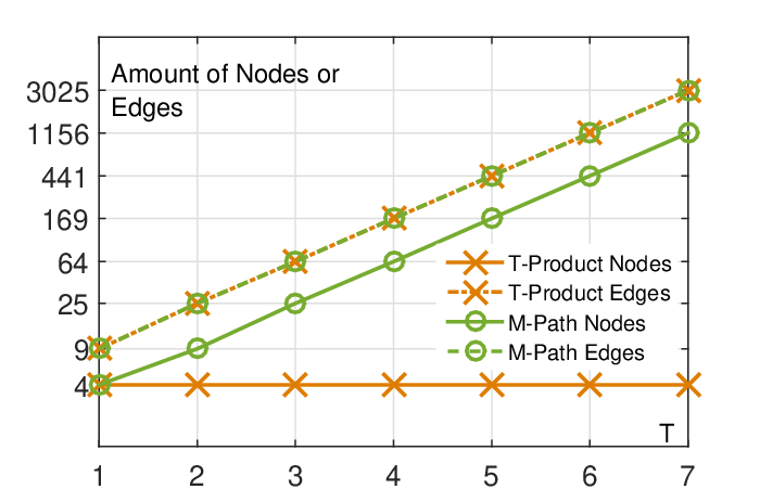
The CJSR estimation $\gamma_{*}(S^{T})$ obtained by applying Theorem 10 to the system $S^{T}(\mathbf{G},\mathbf{\Sigma})$ satisfies $\hat{\rho}(S)\leq\gamma_{*}(S^{T})^{1/T}\leq(1+r)\hat{\rho}(S).$

As a conclusion, given $r>0$ , there is a $T$ -product lift of $S$ allowing the retrieve an estimate with relative error at most $1+r$ . The amount of edges in the system $S^{T}$ increases exponentially with $T$ , with one edge per path of length $T$ . The amount of edges $N_{E}$ of $\mathbf{G}$ has however the least impact for computational complexity (10).

3.2 Approximation through sum-of-squares.

In this subsection we generalize the technique presented in [27] to constrained switching systems and devise a CJSR approximation scheme relying on an algebraic lifting of the set of matrices $\mathbf{\Sigma}$ . The procedure generating the lifted space is called the [ $d$ ]-lift (a full presentation can be found in [27], Section 3). Given an integer $d$ , the [ $d$ ]-lift of a vector $x\in\mathbb{R}^{n}$ is a vector $x^{[d]}\in\mathbb{R}^{C(n+d-1,d)}$ of monomials of degree $d$ , where ${C(k,\ell)}$ is the number of combinations of $\ell$ elements in a set of $k$ elements. More important to us is that the [d]-lift is well defined for linear maps, i.e. $\exists A^{[d]}:A^{[d]}x^{[d]}=(Ax)^{[d]}$ , this definition extends to sets of matrices $\mathbf{\Sigma}^{[d]}$ . Moreover, $\left|x^{[d]}\right|=|x|^{d}$ for the Euclidean norm in the appropriate dimensions.
In constrast with the method of Subsection 3.1, we now conserve the graph of the constrained system, but approximate its CJSR by using potentially non-convex approximations of multinorms that are obtained from homogeneous sum-of-squares polynomials with degree $2d$ , $d\geq 1$ being an integer to be chosen. These polynomials have the form $x\mapsto(x^{[d]})^{\top}Qx^{[d]}$ , where $Q\succ 0$ is a quadratic form in the lifted space.

Theorem 3.5.

Given a system $S(\mathbf{G},\mathbf{\Sigma})$ and an integer $d\geq 1$ , let $S^{[d]}(\mathbf{G},\mathbf{\Sigma})$ denote the constrained switching system on the same graph $\mathbf{G}$ and on $[d]$ -lift $\mathbf{\Sigma}^{[d]}$ of $\mathbf{\Sigma}$ .
The value $\gamma_{*}(S^{[d]})$ obtained by applying Theorem 10 to the system $S^{[d]}$ satisfies $\hat{\rho}(S)\leq\gamma_{*}^{1/d}(S^{[d]})\leq C(n+d-1,d)^{1/(2d)}\hat{\rho}(S).$

PROOF.

Since $|x^{[d]}|=|x|^{d}$ holds for the euclidean norm, we have $\hat{\rho}(S^{[d]})=\hat{\rho}(S)^{d}$ from (1). Given the dimension of the set $\mathbf{\Sigma}^{[d]}$ , Theorem 10 produces an estimate such that $\hat{\rho}(S^{[d]})\leq\gamma_{*}\leq C(n+d-1,d)^{1/2}\hat{\rho}(S^{[d]}).$

The transformation here affects the dimension $n$ of the system. As it is shown in [27] - Example 4, the CJSR approximation can be further refined by making use of explicit sum-of-square programming (rather than solving the program of Theorem 10 in the lifted space), but with the same accuracy bounds.

3.3 Improving accuracy by adding memory to the graph.

Path-dependent Lyapunov functions have been introduced by Lee and Dullerud [21] as tools for the stability analysis and control of discrete-time switching systems. The concept, which follows a similar idea to that of Bliman and Ferrari-Trecate [7], is to build a multiple Lyapunov function that associates a different quadratic form to each switching sequence of a length $M\geq 0$ , $M$ being an integer parameter called the memory of the function. The authors showed that, for any stable switching system, there is a finite $M$ such that the system admits a path-dependent Lyapunov function with memory $M$ .
Similar statements can be made about the T-Product lift and the $[d]$ -lift defined in the previous subsections. Indeed, if $\hat{\rho}(S)<1$ and since the approximations are asymptotically tight, there is a finite value $T$ (or $d$ ) for which the approximation algorithm will return an estimate lower then 1. Given this parallel, it is natural to ask whether the methods of [21, 7] present similar approximation bounds to that of Theorems 3.3 and 3.5.
We first define a lifting procedure, adapted from [21, 7], allowing to obtain path-dependent Lyapunov function as quadratic multinorms of an augmented automaton.

Definition 3.6 (M-Path-Dependent Lifting).

Given a system $S(\mathbf{G}(V,E),\mathbf{\Sigma})$ and an integer $M\geq 0$ , the $M$ -Path-Dependent lift of S, denoted $S_{M}(\mathbf{G},\mathbf{\Sigma})$ , is a constrained switching system with the same set of matrices $\mathbf{\Sigma}$ and with an automaton $\mathbf{G}^{\prime}(V^{\prime},E^{\prime})$ which is the same as $\mathbf{G}$ for $M=0$ , and constructed as follows for $M\geq 1$ . Start with $V^{\prime}=\{\}$ , $E^{\prime}=\{\}$ , then:

1.

For each path $p$ of length $M$ in $\mathbf{G}$ , add the node $v_{p}$ in $V^{\prime}$ .
2.

For each path $p$ of length $M+1$ in $\mathbf{G}$ , let $p=(e_{1},\ldots,e_{M+1})$ , where $e_{k}$ is the $kth$ edge of the path. Define $p^{-}=(e_{1},\ldots,e_{M})$ , $p^{+}=(e_{2},\ldots,e_{M+1})$ , and $\sigma_{p}$ as the label of the edge $e_{M+1}$ . Then, add the edge $(v_{p^{-}},v_{p^{+}},\sigma_{p})\in E^{\prime}$ .

Example 4.

Figure 4 presents the 1-Path-Dependent lift $\mathbf{G}^{\prime}$ of the automaton $\mathbf{G}$ of Figure 3(a). There are 4 nodes in $\mathbf{G}^{\prime}$ , one for each edge of $\mathbf{G}$ . For the edge $(v,w,\sigma)$ of $\mathbf{G}$ , we use “ $vw$ ” to refer to the corresponding node in $\mathbf{G}^{\prime}$ . For the edges, consider for example the path of length 2 $\left((b,b,2),(b,a,4)\right)$ in $\mathbf{G}$ . To this path corresponds the edge $(bb,ba,4)$ in $\mathbf{G}^{\prime}$ .

Theorem 3.7.

Given a system $S(\mathbf{G},\mathbf{\Sigma})$ and an integer $T\geq 1$ , let $\gamma_{*}(S^{T})$ and $\gamma_{*}(S_{T-1})$ be the values obtained by applying Theorem 10 to $S^{T}(\mathbf{G},\mathbf{\Sigma})$ and $S_{T-1}(\mathbf{G},\mathbf{\Sigma})$ respectively. The estimates satisfy $\gamma_{*}(S_{T-1})\leq\left(\gamma_{*}(S^{T})\right)^{1/T}.$

PROOF.

For $T=1$ , $S=S_{T-1}=S^{T}$ , so the claim holds. Assume now $T\geq 2$ . We will show that given a quadratic multinorm for $S^{T}$ with value $\gamma^{T}$ , we can always construct a quadratic multinorm for $S_{T-1}$ with value at most $\gamma$ .
We refer to paths by their succession of edges, $p=(e_{1},\ldots,e_{T})$ is a path of length $T$ in $\mathbf{G}$ , and let $e_{k}=(v_{k-1},v_{k},\sigma_{k})$ . A quadratic multinorm with value $\gamma^{T}$ for $S^{T}$ associates a quadratic form $Q\succ 0$ per node in $\mathbf{G}$ such that, for all paths $p$ ,

A_{p}^{\top}Q_{v_{T}}A_{p}-\gamma^{2T}Q_{v_{0}}\preceq 0.

(11)

To the same path $p$ corresponds an edge in the (T-1)-Path-Dependent lift, between a node $v_{\left(e_{1},\ldots,e_{T-1}\right)}$ and a node $v_{\left(e_{2},\ldots,e_{T}\right)}$ . For a quadratic multinorm of $S_{T-1}$ with value $\gamma$ to exist, there must be a quadratic form $Q_{p}\succ 0$ per path $p$ of length $T$ , such that the following holds:

		$\displaystyle A_{\sigma_{T}}^{\top}Q_{(e_{2},\ldots,e_{T})}A_{\sigma_{T}}$		(12)
		$\displaystyle}{\displaystyle-\gamma^{2}Q_{\left(e_{1},\ldots,e_{T-1}\right)}\preceq 0.$		(12)

Letting $R=Q^{-1}$ denote the inverses of the quadratic forms in the corresponding lift, by a Schurr complement, the LMIs (11) are equivalent to

A_{p}R_{v_{0}}A_{p}^{\top}-\gamma^{2T}R_{v_{T}},\preceq 0,

(13)

and the LMIs (12) to

		$\displaystyle A_{\sigma_{T}}R_{\left(e_{1},\ldots,e_{T-1}\right)}A_{\sigma_{T}}^{\top}$		(14)
		$\displaystyle}{\displaystyle-\gamma^{2}R_{\left(e_{2},\ldots,e_{T}\right)}\preceq 0.$		(14)

Assume that we have a solution $\{R_{v},v\in V\}$ to (13). Given any path $p=(e_{1},\ldots,e_{T-1})$ , with labels $\sigma_{1},\ldots,\sigma_{T-1}$ that visits the nodes $v_{0},\ldots,v_{T-1}$ in $\mathbf{G}$ , define

		$\displaystyle R_{\left(e_{1},\ldots,e_{T-1}\right)}=R_{v_{T-1}}$
		$\displaystyle+\gamma^{-2}A_{\sigma_{T-1}}R_{v_{T-2}}A_{\sigma_{T-1}}^{\top}$
		$\displaystyle}{\displaystyle+\gamma^{-4}A_{\left(\sigma_{T-2},\sigma_{T-1}\right)}R_{v_{T-3}}A^{\top}_{\left(\sigma_{T-2},\sigma_{T-1}\right)}$
		$\displaystyle}{\displaystyle+\cdots$
		$\displaystyle}{\displaystyle+\gamma^{-2(T-1)}A_{\left(\sigma_{1},\ldots,\sigma_{T-1}\right)}R_{v_{0}}A^{\top}_{\left(\sigma_{1},\ldots,\sigma_{T-1}\right)},$

where $A_{(\sigma_{k},\ldots,\sigma_{T-1})}=A_{\sigma_{T-1}}\cdots A_{\sigma_{k}}$ . Injecting these quadratic forms in (14), we obtain (13), and thus we have a quadratic multinorm for $S_{T-1}$ , with value at most $\gamma$ .

Corollary 3.8.

Given a system $S(\mathbf{G},\mathbf{\Sigma})$ and an integer $M\geq 1$ , the value $\gamma_{*}$ obtained by applying Theorem 10 to the $M$ -Path-Dependent lift of S satisfies $\hat{\rho}(S)\leq\gamma_{*}\leq n^{1/(2(M+1))}\hat{\rho}(S).$

The amount of nodes $N_{V}$ and edges $N_{E}$ in the M-Path-Dependent lift both grow exponentially with $M$ , with one node per path of length $M$ , and one edge per path of length $M+1$ in $\mathbf{G}$ .

3.4 A sufficient condition for extremality of quadratic multinorms.

We now present an easy to check sufficient condition under which the CJSR estimate obtained by applying Theorem 10 is exact. The condition can be applied for all the lifts developed above, since they all rely on Theorem 10 to retrieve a quadratic multinorm of minimal value. We assume that the estimate of Theorem 10 is attained by the value of a quadratic multinorm, and give a sufficient condition for its extremality. We start with the following observation.

Lemma 3.9.

For any system $S(\mathbf{G},\mathbf{\Sigma})$ and any cycle²² 2 A cycle is a closed path, i.e. whose source and destination nodes are the same. $c$ of length $T$ in $\mathbf{G}$ , $\hat{\rho}(S)\geq\rho(A_{c})^{1/T}$ , where $\rho(A_{c})$ is the spectral radius of the product $A_{c}$ .

PROOF.

For any induced matrix norm $\|\cdot\|$ , the following holds ρ(A c ) 1/T = lim k →∞ ∥A c k ∥ 1/kT ≤lim k →∞ max{∥A p ∥ 1/kT : p is a path of length $kT$ }, ≤ ^ ρ (S).

We now define a simple cycle in the graph $\mathbf{G}$ as a cycle such that for every node $v$ visited by the cycle, there exists no partition of the cycle into two cycles on $v$ .

Theorem 3.10 (Sufficient extremality condition).

Let $\{Q_{v},\,v\in V\}$ be the optimal quadratic forms obtained by applying Theorem 10 to the system $S(\mathbf{G}(V,E),\mathbf{\Sigma})$ , corresponding to a multinorm $\mathcal{H}$ with value $\gamma_{*}$ . If the set of edges

E^{\prime}=\left\{(v,w,\sigma)\in E:\lambda_{\min}\left(-A_{\sigma}^{\top}Q_{w}A_{\sigma}+\gamma^{2}_{*}Q_{v}\right)=0\right\},

where $\lambda_{\min}(X)$ denotes the smallest eigenvalue of the positive definite matrix $X$ , forms a simple cycle $c$ in $\mathbf{G}$ , then $\mathcal{H}$ is extremal, and $\hat{\rho}(S)=\rho(A_{c})^{1/T},$ where $T$ is the length of $c$ .

PROOF.

The edges in the set $E^{\prime}$ are those for which the LMI constraints in (8) are tight for the multinorm $\mathcal{H}$ . It is a known fact of convex optimization that removing constraints that are not tight at the optimal solution of a given program does not affect its optimal solutions. Therefore, it must be the case that the optimal values $\gamma_{*}$ and $\gamma_{*}^{\prime}$ obtained by applying Theorem 10 respectively to $S(\mathbf{G}(V,E),\mathbf{\Sigma})$ and $S(\mathbf{G}(V,E^{\prime}),\mathbf{\Sigma})$ are equal, and we may focus on the second system.
Since $\mathbf{G}(V,E^{\prime})$ is a simple cycle, then for any $M\geq 0$ , the M-Path-Dependent lift (Definition 3.6) leaves the graph invariant. Applying Corollary 3.8 with $M\rightarrow\infty$ , we conclude that the multinorm obtained from applying Theorem 10 to $S(\mathbf{G}(V,E^{\prime}),\mathbf{\Sigma})$ needs to be extremal for this cyclic graph, and $\gamma_{*}^{\prime}=\rho(A_{c})^{1/T}$ .
Having computed $\gamma_{*}^{\prime}$ , and since $\gamma_{*}=\gamma^{\prime}_{*}$ , we now consider the original system. Applying Lemma 2 and Proposition 4, we get $\rho(A_{c})^{1/T}\leq\hat{\rho}(\mathbf{G},\mathbf{\Sigma})\leq\gamma_{*}=\rho(A_{c})^{1/T},$ which concludes the proof.

3.5 The Kroenecker lift

We end this section by presenting another approach to the stability analysis of constrained switching systems. Kozyakin [18] and Wang [33] independently introduced a lifting procedure that allows to obtain, from any system $S$ , a set of matrices $\mathbf{\Sigma}_{S}$ such that $\hat{\rho}(S)=\hat{\rho}(\mathbf{\Sigma}_{S})$ .

Definition 3.11 (Kroenecker lift).

Given a system $S(\mathbf{G}(V,E),\mathbf{\Sigma})$ , with $N_{V}$ nodes $\{v_{i}\in V,\,1\leq i\leq N_{V}\}$ and $\mathbf{\Sigma}\subset\mathbb{R}^{n\times n}$ , the Kroenecker lift of $S$ is a matrix set defined as $\mathbf{\Sigma}_{\mathbf{G}}=\{A_{(v_{i},v_{j},\sigma)},\,(v_{i},v_{j},\sigma)\in E\},$ with for the edge $(v_{i},v_{j},\sigma)$ ,

A_{(v_{i},v_{j},\sigma)}=\left(\mathbf{e}(j)\mathbf{e}(i)^{\top}\right)\otimes A_{\sigma},

where $\mathbf{e}(k)\in\mathbb{R}^{N_{V}}$ is the $k$ th vector of the canonical basis of $\mathbb{R}^{N_{V}}$ , and $\otimes$ is the Kroenecker product.

The methods in Subsection 3.1, 3.2 and 3.3 are based on the ones of [8, 21, 27] and make use of the concept of multinorm for providing estimates of $\hat{\rho}(S)$ . It is natural to compare these methods with a direct application of the ones of [8, 21, 27] for approximating $\hat{\rho}(\mathbf{\Sigma}_{\mathbf{G}})$ . We will focus on [8], which approximates the JSR of a set of matrices using Theorem 10 with a single quadratic form. The conclusions naturally carry on to the other methods of [27, 21].

Proposition 3.12.

Consider a system $S(\mathbf{G}(V,E),\mathbf{\Sigma})$ and its associated set $\mathbf{\Sigma}_{\mathbf{G}}$ . There exists $Q_{\mathbf{G}}\succ 0$ and $\gamma>0$ such that $\forall A_{(v,w,\sigma)}\in\mathbf{\Sigma}_{S}$ ,

A_{(v,w,\sigma)}^{\top}Q_{\mathbf{G}}A_{(v,w,\sigma)}-\gamma^{2}Q_{\mathbf{G}}\preceq 0,

if and only if $S$ has a quadratic multinorm with value at most $\gamma$ .

PROOF.

Assume without loss of generality that $\gamma=1$ . To ease the reading, we assume $n=1$ , so that for $e\in E$ , $A_{e}\in\mathbb{R}^{N_{V}\times N_{V}}$ . For $e=(v,w,\sigma)\in E$ , we let $B_{e}=A_{e}^{\top}Q_{\mathbf{G}}A_{e}-Q_{\mathbf{G}}$ . The element at row $k$ and column $\ell$ of $A_{e}$ is $A_{e}^{[k,\ell]}$ , and $B_{e}^{[k,\ell]}$ , $Q_{\mathbf{G}}^{[k,\ell]}$ are defined similarly. Define the set of nodes as $\{v_{i}\in V,\,1\leq i\leq N_{V}\}$ . For any $1\leq k,\ell\leq N_{V}$ , we have

	$\displaystyle B_{(v_{i},v_{j},\sigma)}^{[k,\ell]}$	$\displaystyle=\sum_{i^{\prime},j^{\prime}}A_{(v_{i},v_{j},\sigma)}^{\top,[k,i^{\prime}]}Q_{{\mathbf{G}}}^{[i^{\prime},j^{\prime}]}A_{(v_{i},v_{j},\sigma)}^{[j^{\prime},\ell]}-Q_{{\mathbf{G}}}^{[k,\ell]},$
		$\displaystyle=\delta_{k,i}\delta_{\ell,i}\left(A_{(v_{i},v_{j},\sigma)}^{\top,[k,j]}Q_{{\mathbf{G}}}^{[j,j]}A_{(v_{i},v_{j},\sigma)}^{[j,\ell]}\right)-Q_{{\mathbf{G}}}^{[k,\ell]},$

where $\delta_{i,j}=1$ if and only if $i=j$ (Kroenecker delta).
For the only if part, $Q_{\mathbf{G}}\succ 0$ and $B_{e}\preceq 0$ . Since $Q_{\mathbf{G}}\succ 0$ and $B_{e}\preceq 0$ , then for all $1\leq k\leq N_{V}$ , $Q_{\mathbf{G}}^{[k,k]}>0$ , and for any $e=(v_{i},v_{j},\sigma)\in E$ , $B^{[i,i]}_{e}=A^{\top}_{\sigma}Q_{\mathbf{G}}^{[j,j]}A_{\sigma}-Q_{\mathbf{G}}^{[i,i]}\leq 0.$ Thus, we extract a quadratic multinorm for $S$ using the quadratic forms $Q_{\mathbf{G}}^{[i,i]}$ , $1\leq i\leq N_{V}$
For the if part of the proof, we take quadratic multinorm with value lower than 1. Let $Q_{i}>0,1\leq i\leq N_{V}$ , be the quadratic forms associated at each node. We reconstruct $Q_{\mathbf{G}}$ by setting $Q_{\mathbf{G}}^{[k,\ell]}=Q_{k}$ if $k=\ell$ , and $Q_{\mathbf{G}}^{[k,\ell]}=0$ else.

Applying Theorem 3.1 to $\mathbf{\Sigma}_{\mathbf{G}}$ therefore produces the same estimate as if it was applied on $S$ . However, when using $\mathbf{\Sigma}_{\mathbf{G}}\subset\mathbb{R}^{nN_{V}\times nN_{V}}$ , the complexity (10) reads $\mathcal{O}\left((nN_{V})^{(13/2)}N_{E}^{(3/2)}\right)$ , a significant increase compared to the previous $\mathcal{O}\left(n^{(13/2)}N_{V}^{(7/2)}N_{E}^{(3/2)}\right)$ . Moreover, the accuracy bounds (9) become worse, due to the larger dimension of $\mathbf{\Sigma}_{\mathbf{G}}$ .

4 Numerical example

We consider the dynamics of a plant that may experience controller failures: $x_{t+1}=\left(A+BK_{\sigma(t)}\right)x_{t},$ with

A=\begin{pmatrix}0.94&0.56\\ 0.14&0.46\end{pmatrix},\,B=\begin{pmatrix}0\\ 1\end{pmatrix},

and $K_{\sigma(t)}=(k_{1,\sigma(t)},k_{2,\sigma(t)})$ . The control gains switch to represent 4 failures modes. When everything works as expected, $\sigma(t)=1$ , and

K_{1}=\begin{pmatrix}k_{1}&k_{2}\end{pmatrix}=\begin{pmatrix}-0.49&0.27\end{pmatrix}.

The second and third modes correspond respectively to a failure of the first and second part of the controller, with $K_{2}=(0,k_{2})$ and $K_{3}=(k_{1},0).$ The last mode is the total failure case with $K_{4}=(0,0).$ As a constraint, we consider that a same part of the controller never fails twice in a row. We obtain a constrained switching system on the set $\mathbf{\Sigma}=\{A+BK_{\sigma}\},\,\sigma\in\{1,\ldots,4\},$ with the automaton $\mathbf{G}(V,E)$ depicted in Figure 5.

We first provide increasingly accurate estimates of the CJSR of the system, and then provide the exact value of the CJSR using Theorem 3.10. For the estimations, we compare the T-Product lift of Subsection 3.1, and the M-Path-Dependent lift, introduced in [21] and further studied in Subsection 3.3. We apply these methods for $T=1,\ldots,7$ , and $M=T-1=0,\ldots,6$ . From Corollary 3.4 and Theorem 3.8, these choices produce estimates within $[\hat{\rho}(S),(1+r)\hat{\rho}(S)]$ , with $1+r$ ranging from $\sqrt{2}\simeq 1.41$ for $T=1$ to $2^{1/14}\simeq 1.05$ for $T=7$ .
For each value of $T$ and $M$ we first compute the lifted systems $S^{T}$ and $S_{M}$ . Figure 6 provides a comparison of the amount of nodes and edges of these systems. Then, we solve the optimization program of Theorem 10 on the lifts, applying Theorems 3.3 and 3.7 to obtain bounds on the CJSR.³³ 3 Matlab codes reproducing the results available at
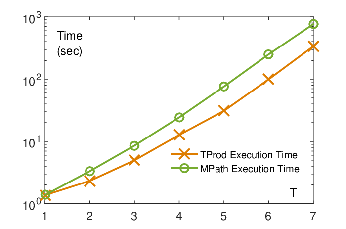
“http://sites.uclouvain.be/scsse/postrev.zip”. The execution times for producing the estimates are compared in Figure 7, and the estimation values are compared in Figure 8. The best estimation is achieved with the $M$ -Path-Dependent lift, for $M=6$ , guaranteeing that $\hat{\rho}(S)\leq 0.9748\ldots.$ However, the T-Product lift provides estimates much faster.

We now use Theorem 3.10 for computing the exact value of the CJSR. The results of Figure 8 indicate that the sufficient condition can only be met by the M-Path-Dependent lift, for $M=T-1=4,5$ or $6$ . In this case, for $M=5$ , the conditions of Theorem 3.10 are met. The obtained simple cycle corresponds to the switching sequence repeating the labels $\{2,3,1,1,1,1,2,1\}$ and reaches the CJSR. Indeed, we have (Lemma 2)

\displaystyle\hat{\rho}(S)

\displaystyle\geq\rho(A_{1}A_{2}A_{1}^{4}A_{3}A_{2})^{1/8}\simeq 0.9478\ldots,

which matches our best CJSR estimate.

5 Conclusion

We established a new framework for the stability analysis of discrete-time linear switching systems with constrained switching sequences. It relies around the newly introduced concept of multinorms and their link to the constrained joint spectral radius [11] (CJSR). The stability of constrained switching systems is equivalent to the existence of a set of exactly one norm per node of the automaton, with contractivity relations that are given by the edges of the automaton.
By approximating these norms individually with quadratic norms, we design the first arbitrarily accurate CJSR approximation schemes. The framework also encapsulate well-known methods such as path-dependent Lyapunov functions [21, 7] as methods approximating extremal multinorms.
In the future, we will apply this framework to control-oriented problems. Path-dependent Lyapunov functions have been used in feedback controller design [21, 12], and our goal is now to give guarantees on the performance of these controllers. Their usage for the study of the contractiveness of switching systems [20, 12] suggests an estimation framework in this setting.

References

[1] A. A. Agrachev and D. Liberzon, “Lie-algebraic stability criteria for switched systems,” SIAM Journal on Control and Optimization, vol. 40, no. 1, pp. 253–269, 2001.
[2] A. A. Ahmadi, “Algebraic relaxations and hardness results in polynomial optimization and lyapunov analysis,” Ph.D. dissertation, Massachusetts Institute of Technology, 2011.
[3] A. A. Ahmadi, R. M. Jungers, P. A. Parrilo, and M. Roozbehani, “Joint spectral radius and path-complete graph lyapunov functions,” SIAM Journal on Control and Optimization, vol. 52, no. 1, pp. 687–717, 2014.
[4] T. Ando and M.-H. Shih, “Simultaneous contractibility,” SIAM Journal on Matrix Analysis and Applications, 19(2), 487-498, 1998.
[5] N. Athanasopoulos and M. Lazar, “Alternative stability conditions for switched discrete time linear systems,” in IFAC World Congress, 2014, pp. 6007–6012.
[6] A. Ben-Tal and A. Nemirovski, Lectures on modern convex optimization: analysis, algorithms, and engineering applications. Siam, 2001, vol. 2.
[7] P.-A. Bliman and G. Ferrari-Trecate, “Stability analysis of discrete-time switched systems through lyapunov functions with nonminimal state,” in Proceedings of IFAC Conference on the Analysis and Design of Hybrid Systems, 2003, pp. 325–330.
[8] V. D. Blondel, Y. Nesterov, and J. Theys, “On the accuracy of the ellipsoid norm approximation of the joint spectral radius,” Linear Algebra and its Applications, vol. 394, pp. 91–107, 2005.
[9] M. S. Branicky, “Multiple lyapunov functions and other analysis tools for switched and hybrid systems,” IEEE Transactions on Automatic Control, vol. 43, no. 4, pp. 475–482, 1998.
[10] J. Daafouz, P. Riedinger, and C. Iung, “Stability analysis and control synthesis for switched systems: a switched lyapunov function approach,” IEEE Transactions on Automatic Control, vol. 47, no. 11, pp. 1883–1887, 2002.
[11] X. Dai, “A Gel’fand-type spectral radius formula and stability of linear constrained switching systems,” Linear Algebra and its Applications, vol. 436, no. 5, pp. 1099–1113, 2012.
[12] R. Essick, J.-W. Lee, and G. E. Dullerud, “Control of linear switched systems with receding horizon modal information,” IEEE Transactions on Automatic Control, vol. 59, no. 9, pp. 2340–2352, 2014.
[13] E. A. Hernandez-Vargas, R. H. Middleton, and P. Colaneri, “Optimal and mpc switching strategies for mitigating viral mutation and escape,” in Proc. of the 18th IFAC World Congress Milano (Italy) August, 2011.
[14] F. John, “Extremum problems with inequalities as subsidiary conditions,” in Traces and Emergence of Nonlinear Programming (197–215). Springer, 2014.
[15] R. Jungers, “The joint spectral radius,” Lecture Notes in Control and Information Sciences, vol. 385, 2009.
[16] R. M. Jungers, A. D’Innocenzo, and M. D. Di Benedetto, “Feedback stabilization of dynamical systems with switched delays,” in Proc. of the 51st IEEE Conference on Decision and Control, 2012, pp. 1325–1330.
[17] R. M. Jungers and W. M. Heemels, “Controllability of linear systems subject to packet losses,” preprint at www.heemels.tue.nl/content/papers/JunHee $\_$ ADHS15a.pdf.
[18] V. Kozyakin, “The Berger–Wang formula for the markovian joint spectral radius,” Linear Algebra and its Applications, vol. 448, pp. 315–328, 2014.
[19] A. Kundu and D. Chatterjee, “Stabilizing switching signals for switched systems,” IEEE Transactions on Automatic Control,, vol. 60, no. 3, pp. 882–888, 2015.
[20] J.-W. Lee and G. E. Dullerud, “Optimal disturbance attenuation for discrete-time switched and markovian jump linear systems,” SIAM Journal on Control and Optimization, vol. 45, no. 4, pp. 1329–1358, 2006.
[21] ——, “Uniform stabilization of discrete-time switched and markovian jump linear systems,” Automatica, 42(2), 205-218, 2006.
[22] J.-W. Lee and P. P. Khargonekar, “Detectability and stabilizability of discrete-time switched linear systems,” IEEE Transactions on Automatic Control, vol. 54, no. 3, pp. 424–437, 2009.
[23] D. Liberzon and A. S. Morse, “Basic problems in stability and design of switched systems,” IEEE Control Systems Magazine, vol. 19, no. 5, pp. 59–70, 1999.
[24] H. Lin and P. J. Antsaklis, “Stability and stabilizability of switched linear systems: a survey of recent results,” IEEE Transactions on Automatic control, vol. 54, no. 2, pp. 308–322, 2009.
[25] M. Lothaire, Algebraic combinatorics on words. Cambridge University Press, 2002, vol. 90.
[26] R. Olfati-Saber and R. M. Murray, “Consensus problems in networks of agents with switching topology and time-delays,” IEEE Transactions on Automatic Control, vol. 49, no. 9, pp. 1520–1533, 2004.
[27] P. A. Parrilo and A. Jadbabaie, “Approximation of the joint spectral radius using sum of squares,” Linear Algebra and its Applications, vol. 428, no. 10, pp. 2385–2402, 2008.
[28] M. Philippe and R. M. Jungers, “Converse lyapunov theorems for discrete-time linear switching systems with regular switching sequences,” in Proceedings of the 14th European Control Conference, Linz, 2015.
[29] ——, “A sufficient condition for the boundedness of matrix products accepted by an automaton,” in Proceedings of the 18th International Conference on Hybrid Systems: Computation and Control. ACM, 2015, pp. 51–57.
[30] G.-C. Rota and W. Strang, “A note on the joint spectral radius,” Nederlandse Koninklÿ ke Akademie & van Wetenschappen Indagationes Mathematicae, 22, 379-381, 1960.
[31] R. Shorten, F. Wirth, O. Mason, K. Wulff, and C. King, “Stability criteria for switched and hybrid systems,” SIAM review, vol. 49, no. 4, pp. 545–592, 2007.
[32] G. Vankeerberghen, J. Hendrickx, and R. M. Jungers, “Jsr: a toolbox to compute the joint spectral radius,” in Proceedings of the 17th international conference on Hybrid systems: computation and control. ACM, 2014, pp. 151–156.
[33] Y. Wang, N. Roohi, G. E. Dullerud, and M. Viswanathan, “Stability of linear autonomous systems under regular switching sequences,” in Proc. of the 53rd IEEE Conference on Decision and Control, 2014, pp. 5445–5450.

6 Annex: Proof of Theorem 1.1

From Definition 2 in [11], we know that the limit (1) converges. Since the limit (1) converges, $\forall\epsilon>0,\,\exists T_{\epsilon}\geq 0:\,\forall t\geq T_{\epsilon}$ ,

\hat{\rho}(S)^{t}\leq\max_{\sigma({\cdot})\,\text{accepted by $\mathbf{G}$}}\|A_{\sigma(t-1)}\cdots A_{\sigma(0)}\|\leq(\hat{\rho}(S)+\epsilon)^{t}.

To show that $\hat{\rho}(S)<1$ implies (exponential) stability, it suffice to take $\epsilon<1-\hat{\rho}(S)$ . Indeed, we then get that for all accepted sequences, $\lim_{t\rightarrow\infty}\|A_{\sigma(t-1)}\cdots A_{\sigma(0)}\|=0.$ Exponential stability is then acquired since there can only be a finite amount of products of length $t\leq T_{\epsilon}$ with $\|A_{\sigma(t-1)}\ldots A_{\sigma(t)}\|>(\hat{\rho}(S)+\epsilon)^{t}$ .
Consider now the case $\hat{\rho}(S)\geq 1$ . For all $t\geq 1$ , we define $x_{*}^{t}$ as

x_{*}^{t}=\text{arg}\max_{|x|=1}\max_{\sigma({\cdot})\,\text{accepted by $\mathbf{G}$}}|A_{\sigma(t-1)}\cdots A_{\sigma(0)}x|.

We extract from the sequence $\{x_{*}^{t}\}_{t\geq 1}$ a subsequence converging to a point $x_{*}$ , $|x_{*}|=1$ . From this point, there is a switching sequence satisfying $\lim_{t\rightarrow\infty}|A_{\sigma(t-1)}\cdots A_{\sigma(0)}x_{*}|\geq 1/2.$ Thus, the system is not asymptotically stable when $\hat{\rho}(S)\geq 1$ .
This concludes the proof of Theorem 1.1.

$\displaystyle\|x\|_{v}$	$\displaystyle=\sup_{p}\{\|{A}_{p}^{\prime}x\|:p\text{ is a path with origin $v$}\},$
	$\displaystyle\geq\sup_{q}\{\|{A}_{q}^{\prime}A^{\prime}_{\sigma}x\|:q\text{ is a path with origin $w$}\},$	(6)
	$\displaystyle=\|A^{\prime}_{\sigma}x\|_{w},$

Stability of discrete-time switching systems with constrained switching sequences.

Abstract

keywords

1 Introduction

Theorem 1.1 (Dai [11], Corollary 2.8)

2 Lyapunov functions for constrained switching systems

Proposition 2.1 (e.g. [15], Proposition 1.4)

Example 1.

Definition 2.2 (Multinorm).

Proposition 2.3.

PROOF.

Theorem 2.4.

Example 2.

2.1 Extremal multinorms and boundedness

Theorem 2.5.

PROOF.

3 Approximation algorithms for stability analysis

Theorem 3.1.

PROOF.

3.1 The TT-product lift

Definition 3.2 (TT-product lift).

Example 3.

Theorem 3.3.

PROOF.

Corollary 3.4.

3.2 Approximation through sum-of-squares.

Theorem 3.5.

PROOF.

3.3 Improving accuracy by adding memory to the graph.

Definition 3.6 (M-Path-Dependent Lifting).

Example 4.

Theorem 3.7.

PROOF.

Corollary 3.8.

3.4 A sufficient condition for extremality of quadratic multinorms.

Lemma 3.9.

PROOF.

Theorem 3.10 (Sufficient extremality condition).

PROOF.

3.5 The Kroenecker lift

Definition 3.11 (Kroenecker lift).

Proposition 3.12.

PROOF.

4 Numerical example

5 Conclusion

References

6 Annex: Proof of Theorem 1.1

3.1 The $T$ -product lift

Definition 3.2 ( $T$ -product lift).