Video-Based Action Recognition Using Rate-Invariant Analysis of Covariance Trajectories
Abstract
Statistical classification of actions in videos is mostly performed by extracting relevant features, particularly covariance features, from image frames and studying time series associated with temporal evolutions of these features. A natural mathematical representation of activity videos is in form of parameterized trajectories on the covariance manifold, i.e. the set of symmetric, positive-definite matrices (SPDMs). The variable execution-rates of actions implies variable parameterizations of the resulting trajectories, and complicates their classification. Since action classes are invariant to execution rates, one requires rate-invariant metrics for comparing trajectories. A recent paper represented trajectories using their transported square-root vector fields (TSRVFs), defined by parallel translating scaled-velocity vectors of trajectories to a reference tangent space on the manifold. To avoid arbitrariness of selecting the reference and to reduce distortion introduced during this mapping, we develop a purely intrinsic approach where SPDM trajectories are represented by redefining their TSRVFs at the starting points of the trajectories, and analyzed as elements of a vector bundle on the manifold. Using a natural Riemannain metric on vector bundles of SPDMs, we compute geodesic paths and geodesic distances between trajectories in the quotient space of this vector bundle, with respect to the re-parameterization group. This makes the resulting comparison of trajectories invariant to their re-parameterization. We demonstrate this framework on two applications involving video classification: visual speech recognition or lip-reading and hand-gesture recognition. In both cases we achieve results either comparable to or better than the current literature.
Keywords: Action recognition, covariance manifold, trajectories on manifolds, vector bundles, rate-invariant classification
1 Introduction
The problem of classification of human actions or activities in video sequences is both important and challenging. It has applications in video surveillance, lip reading, pedestrian tracking, hand-gesture recognition, manufacturing quality control, human-machine interfaces, and so on. Since the size of video data is generally very high, the task of video classification is often performed by extracting certain low-dimensional features of interest – geometric, motion, colorimetric features, etc – from each frame and then forming temporal sequences of these features for full videos. Consequently, analysis of videos get replaced by modeling and classification of longitudinal observations in a certain feature space. (Some papers discard temporal structure by pooling all feature together but that represents a severe loos of information.) Since many features are naturally constrained to lie on nonlinear manifolds, the corresponding video representations form parameterized trajectories on these manifolds. Examples of these manifolds include unit spheres, Grassmann manifolds, tensor manifolds, and the space of probability distributions.
One of the most commonly used and effective feature in image analysis is a covariance matrix, as shown via applications in medical imaging [1, 2] and computer vision [3, 4, 5, 6, 7, 8]. These matrices are naturally constrained to be symmetric positive-definite matrices (SPDMs) and have also played a prominent role as region descriptors in texture classification, object detection, object tracking, action recognition and face recognition. Tuzel et al. [3] introduced the concept of covariance tracking where they extracted a covariance matrix for each video frame and studied the temporal evolution of this matrix in the context of pedestrian tracking in videos. Since the set of SPDMs is a nonlinear manifold, denoted by , a whole video segment can be represented as a (parameterized) trajectory on . In this paper we focus on the problem of classification of actions or activities by treating them as parameterized trajectories on . The two specific applications we will study are: visual-speech recognition and hand-gesture classification. Fig. 1 illustrates examples of video frames for these two applications.
One challenge in characterizing activities as trajectories comes from the variability in execution rates. The execution rate of an activity dictates the parameterization of the corresponding trajectory. Even for the same activity performed by the same person, the execution rates can potentially differ a lot. Different execution rate implies that the corresponding trajectories go through the same sequences of points in but have different parameterizations. Directly analyzing such trajectories without alignment, e.g. comparing the difference, calculating point-wise mean and covariance, can be misleading (the mean is not representative of individual trajectories, and the variance is artificially inflated).
 |
To make these issues precise, we develop some notation first. Let be a trajectory and let be a positive diffeomorphism such that and . This plays the role of a time-warping function, or a re-parameterization function, so that the composition is now a time-warped or re-parameterized version of . In other words, the trajectory goes through the same set of points as but at a different rate (speed).
- 1.
Pairwise Registration: Now, let be two trajectories on . The process of registration of and is to find a warping such that is optimally registered to for all . In order to ascribe a meaning to optimality, we need to develop a precise criterion.
- 2.
Groupwise or Multiple Registration: This problem can be extended to more than two trajectories: let be trajectories on , and we want to find out time warpings such that for all , the variables are optimally registered. A solution for pairwise registration can be extended to the multiple alignment problem as follows – for the given trajectories, first define a template trajectory and then align each given trajectory to this template in a pairwise fashion. One way of defining this template is to use the mean of given trajectories under an appropriately chosen metric.
Notice that the problem of comparisons of trajectories is different from the problem of curve fitting or trajectory estimation from noisy data. Many papers have studied spline-type solutions for fitting curves to discrete, noisy data points on manifolds [9, 10, 11, 12, 13] but in this paper we assume that the trajectories are already available through some other means.
1.1 Past Work & Their Limitations
There are very few papers in the literature for analyzing, in the sense of comparing, averaging or clustering, trajectories on nonlinear manifolds. Let denote the geodesic distance resulting from the chosen Riemannian metric on . It can be shown that the quantity forms a proper distance on the set , the space of all trajectories on . For example, [14] uses this metric, combined with the arc-length distance on , to cluster hurricane tracks. However, this metric is not immune to different temporal evolutions of hurricane tracks. Handling this variability requires performing some kind of temporal alignment. It is tempting to use the following modification of this distance to align two trajectories:
| (1) |
but this can lead to degenerate solutions (also known as the pinching problem, described for real-valued functions in [15]). Pinching implies that a severely distorted is used to eliminate (or minimize) those parts of that do not match with , which can be done even when is mostly different from . While this degeneracy can be avoided using a regularization penalty on , some of the other problems remain, including the fact that the solution is not symmetric.
A recent solution, presented in [16, 4], develops the concept of elastic trajectories to deal with the parameterization variability. It represents each trajectory by its transported square-root vector field (TSRVF) defined as:
where is pre-determined reference point on and denotes a parallel transport of the vector from the point to along a geodesic path. This way a trajectory can be mapped into the tangent space and one can compare/align them using the norm on that vector space. More precisely, the quantity provides not only a criterion for optimality of but also approximates a proper metric for averaging and other statistical analyses. (The exact metric is based on the use of semigroup , the set of all absolutely continuous, weakly increasing functions, rather than . We refer the reader to [16] for details.) This TSRVF representation is an extension of the SRVF used for elastic shape analysis of curves in Euclidean spaces [17]. One limitation of this framework is that the choice of reference point, , is left arbitrary. The results can potentially change with and make it difficult to interpret the results. A related, and bigger issue, is that the transport of tangent vectors to , along geodesics, can introduce large distortion, especially when the trajectories are far from on the manifold.
1.2 Our Approach
We present a different approach that does not require a choice of . Here the trajectories are represented by their transported vector fields but without a need to transport them to a global reference point. For each trajectory , the reference point is chosen to be its starting point , and the transport is performed along the trajectory itself. In other words, for each , the velocity vector is transported along to the tangent space of the starting point . This idea has been used previously in [11] and others for mapping trajectories into vector spaces, and results in a relatively stable curve, with smaller distortion than the TSRVFs of [16]. We then develop a metric-based framework for comparing, averaging, and modeling such curves in a manner that is invariant to their re-parameterizations. Consequently, this framework provides a natural solution for removal of rate, or phase, variability from trajectory data.
Another issue is the choice of Riemannian metric on . Although a larger number of Riemannian structures and metrics have been used for in past papers and books [18, 19], they do not provide all the mathematical tools we will need for ensuing statistical analysis. Consequently, we use a different Riemannian structure than those previous papers, a structure that allows relevant mathematical tools for applying the proposed framework.
The rest of this paper paper is organized as follows. In Section 3, we introduce a framework of aligning, averaging and comparing of trajectories on a general manifold . Since we mainly focus on , in Section 2, we introduce the details of the Riemannian structure on used to implement the comparison framework described in Section 3. In Section 4, we demonstrate the proposed work with real-world action recognition data involving two applications: lip-reading and hand-gesture recognition.
2 Riemannian Structure on
Here we will discuss the geometry of and impose a Riemannian structure that facilitates our analysis of trajectories on . Most of the background material is derived in Appendix A with only the final expressions noted here. For a beginning reader in differential geometry, we strongly recommend reading Appendix A first.
We start by choosing an appropriate Riemannian metric on . Then, from the resulting structure, we derive expressions for the following: (1) geodesic paths between arbitrary points on ; (2) parallel transport of tangent vectors along geodesic paths; (3) exponential map; (4) inverse exponential map; and (5) Riemannian curvature tensor. Several past papers have studied the space of SPDMs as a nonlinear manifold and imposed a metric structure on that manifold [2, 1, 18, 20]. While they mostly focus on defining distances, a few of them originate from a Riemannian structure with expressions for geodesics and exponential maps. However, they do not provide expressions for all desired items (parallel transport and Riemannian curvature tensor). In this section, we utilize a particular Riemannian structure on , which is similar but not identical to the one in [2], and is particularly convenient for our purposes. This Riemannian structure has been used previously for other applications such as spline-fitting in [13].
Let be the space of SPDMs, and let be its subset of matrices with determinant one. The tangent spaces of and at , where is the identity matrix, are and . The exponential map at can be shown to be the standard matrix exponential: for any (), there is () such that (), where denotes the matrix (Lie) exponential; this relationship is one-to-one. Our approach is first to identify the space with the quotient space and borrow the Riemannian structure from the latter directly. Then, we straightforwardly extend the Riemannian structure on to . The Riemannian geometries of and its quotient space are discussed in Appendix A. As described there, the Riemannian metric at any point is defined by pulling back the tangent vectors under to , and then using the metric (see Eqn. 8). This definition leads to expressions for exponential map, its inverse, parallel transport of tangent vectors, and the Riemannian curvature tensor on . It also induces a Riemannian structure on the quotient space in a natural way because it is invariant to the action of on .
2.1 Riemannian Structure on
To make the connection with , we state a useful result termed the polar decomposition of square matrices. Recall that for any square matrix , one can decompose it uniquely as where is a SPDM with determinant one and . We note in passing that this fact makes a section of under the action of . (If a group acts on a manifold, then a section of that action is defined to be a subset of the manifold that intersects each orbit of the action in at most one point. It is easy to see that satisfies that condition for the action of on . For any orbit , intersects that orbit in only one point given by such that .) We also note that this section is not an orthogonal section since it is not perpendicular to the orbit, i.e., the tangent space is not perpendicular to the tangent space . We will identify with the quotient space via a map defined as:
for any . One can check that this map is well defined and is a diffeomorphism.
This square-root is the symmetric, positive-definite square-root of a symmetric matrix.
One can verify that lies in
by letting (polar decomposition), and then .
The inverse map of is given by: .
This establishes a one-to-one correspondence between the quotient space and .
We will use the map to push forward the chosen Riemannian metric from the quotient space to .
Geodesic between two points on : With that induced Riemannian metric, we can derive the geodesic path and the geodesic distance between any and in . The idea is to pullback these points into the quotient space using , compute the geodesic there and then map the result back to using . As mentioned earlier and . The expression for geodesic between these points in the quotient space is given in Appendix A. We compute such that for some . (Let . Note that , and the rotation matrix brings to .) The corresponding geodesic in the quotient space () is given by and, therefore, the desired geodesic in is
The corresponding geodesic distance is
Parallel transport of tangent vectors along geodesic paths on : To determine the parallel transport along the geodesic path , we recall from Appendix A that the two orthogonal subspaces of : and , which we call the vertical and the horizontal tangent subspaces, respectively. We identify the tangent space with the horizontal subspace in , so that .
Now let be a tangent vector that needs to be translated along a geodesic path from to , given by . Similar to the case of quotient space in Appendix A, let such that is identified with . In the quotient space, the parallel transport of along the geodesic is a vector field . In , the geodesic is obtained by the forward map , . Therefore, the parallel transport vector field in along the geodesic is the image of under :
where and .
Riemannian curvature tensor on : Let and be three vectors on , then the Riemannian curvature tensor on with these arguments can be calculated in the follows. Let and be elements in such that , and , the tensor is given by:
We summarize these mathematical tools for trajectories analysis on the manifold :
- 1.
Exponential map: Give a point and a tangent vector , the exponential map is given as:
- 2.
Geodesic distance: For any two points , the geodesic distance between them in is given by: where and .
- 3.
Inverse exponential map: For any , the inverse exponential map can be calculated using the formula:
- 4.
Parallel transport: Given and a tangent vector , the tangent vector at which is the parallel transport of along the shortest geodesic from to is: , where and .
- 5.
Riemannian curvature tensor: For any point and tangent vectors and , the Riemannian curvature tensor is given as: , where and .
2.2 Extension of Riemannian Structure to
We now extend the Riemannian structure on to .
Since for any we have , we can express with
. Thus, is identified with the product space of .
Moreover, for any smooth function on , the Riemannian metric , where and denote the Riemannian metrics on and respectively, gives the structure of a “warped” Riemannian product. In this paper we set .
Geodesic between points on : Using the above Riemannian metric () on , the resulting squared distance on between and is:
For two points and , let for some , and , we have . Therefore, the resulting squared geodesic distance between two SPDMs and is
Next, let denote the geodesic in , where is a geodesic on and is a geodesic in . The geodesic from to in is given by
from earlier derivation, and the geodesic , a line segment from to , is
. Therefore, with simple calculation, the matrices in corresponding to the geodesic path are .
Parallel transport of tangent vectors along geodesic paths on :
If is a tangent vector to at , where is identified with and , we can express as with being a tangent vector of at . The parallel transport of is the parallel transport of each of its two components in the corresponding space, and the transport of is itself. The other part, i.e. the parallel translation of in has been dealt earlier.
Riemannian curvature tensor on : By identifying the tangent vector , the non-zero curvature tensors are just the part in . Therefore, the curvature tensor for , and on is the same as .
Again, we summarize these mathematical tools on :
- 1.
Exponential map: Give and a tangent vector . We denote , where , and . The exponential map is given as , where
- 2.
Geodesic distance: For any , the squared geodesic distance between them is : , where .
- 3.
Inverse exponential map: For any , the inverse exponential map , where and .
- 4.
Parallel transport: For any and a tangent vector , the parallel transport of along the geodesic from to is: , where and .
- 5.
Riemannian curvature tensor: For tangent vectors and , the Riemannian curvature tensor is the same as .
2.3 Differences From Past Riemannian Structures
Pennec et al. [2] and others [21, 22, 23] and even others before them have utilized a Riemannian structure on that is commonly known as the Riemanian metric in the literature. Here we clarify the difference between our Riemannian structure and the structure used in these past papers.
We have used a natural bijection given by to inherit the Riemannian structure from the quotient space to . Its inverse is given by . There is another bijection between these same two sets, defined by , and with the inverse . (Note that an element of can be raised to any positive power in a well-defined way by diagonalizing.) If we use to transfer the Riemannian structure from the quotient space onto , we will reach the one used in earlier papers. In other words, the structure on the quotient space is the same for both cases, only the inherited structure on is different due to the different bijections. Note that for all , . It follows that the map from defined by forms an isometry with our metric on one side and the older metric on the other.
The Riemannian metric on (trace metric on pulled-back matrices at identity) is invariant under right translation by elements of and under left translation by elements of . It follows that the induced metric on the quotient space is invariant under the natural left action of on . (This action is given by .) It is a well-known fact that, up to a fixed scalar multiple, this is the only metric on that is invariant under the action by . This aspect is same for both the cases. If we push forward the action of on the quotient space via , the resulting action of on is given by , but if we push forward the action via , the resulting action of on is given by .
Given a simple relationship between the two Riemannian structures, one may conjecture that the relevant formulae (parallel transport, curvature tensor, etc) can be mapped from one setup to another. While this is true in principle, the practice is much harder since it involves the expression for the differential of this map which is somewhat complicated.
3 Analysis of Trajectories on
Now that we have expressions for calculating relevant geometric quantities on , we return to the problem of analyzing trajectories on . In the following we derive the framework for a general Riemannian manifold , keeping in mind that in our applications.
3.1 Representation of Trajectories
Let denote a smooth trajectory on a Riemannian manifold and denote the set of all such trajectories: . Define to be the set of all orientation preserving diffeomorphisms of : is a diffeomorphism. forms a group under the composition operation. If is a trajectory on , then is a trajectory that follows the same sequence of points as but at the evolution rate governed by . More technically, the group acts on , , according to .
We introduce a new representation of trajectories that will be used to compare and register them. We assume that for any two points , we have a mechanism for parallel transporting any vector along from to , denoted by .
Definition 1
Let denote a smooth trajectory starting with . Given a trajectory , and the velocity vector field , define its transported square-root vector field (TSRVF) to be a scaled parallel-transport of the vector field along to the starting point according to: for each , , where denotes the norm that is defined through the Riemannian metric on .
Note the difference in this definition from the one in [16] where the parallel transport was along geodesics to a reference point . Here the parallel transport is along and to the starting point . The concept of parallel transportation of velocity vector along trajectories has also been used previously in [11] and others. This reduces distortion in representation relative to the parallel transport of [16] to a faraway reference point.
This TSRVF representation maps a trajectory on to a curve in . What is the range space of all such mapping? For any point , denote the set of all square-integrable curves in as . The space of interest, then, becomes an infinite-dimensional vector bundle , which is the indexed union of for every . Note that the TSRVF representation is bijective: any trajectory is uniquely represented by a pair , where is the starting point, is its TSRVF. We can reconstruct the trajectory from using the covariant integral defined later (in Algorithm 3).
3.2 Riemannian Structure on
In order to compare trajectories, we will compare their corresponding representations in and that requires a Riemannian structure on the latter space. Let be two trajectories on , with starting points and , respectively, and let the corresponding TSRVFs be and . Now are represented as two points in the vector bundle over . This representation space is an infinite-dimensional bundle, whose fiber over each point in is .
We impose the following Riemannian structure on . For an element in , where , , we naturally identify the tangent space at to be: . To see this, suppose we have a curve in given by , . The velocity vector to this curve at is given by , where denotes , and denotes covariant differentiation of tangent vectors. The Riemannian inner product on is defined in an obvious way: If and are both elements of , define
| (2) |
where the inner products on the right denote the original Riemannian metric in .
Next, for given two points and on , we are interested in finding the geodesic path connecting them. Let be a path with and . We have the following characterization of geodesics on .
Theorem 1
A parameterized path given by on (where the variable corresponds to the parametrization in ), is a geodesic on if and only if:
| (3) |
Here denotes the Riemannian curvature tensor, denotes , and denotes the covariant differentiation of tangent vectors on tangent space .
Proof: We will prove this theorem in two steps.
(1) First, we consider with a simpler case where the space of interest is the tangent bundle of the Riemannian manifold .
An element of is denoted by , where and . It is natural to identify .
The Riemannian inner product on is defined in the obvious way: If and are both elements of , define
and, again, the inner products on the right denote the original Riemannian metric on . Suppose we have a path in given by . We define the energy of this path by
The integrand is the inner product of the velocity vector of the path with itself. It is a standard result that a geodesic on can be characterized as a path that is a critical point of this energy function on the set of all paths between two fixed points in . To derive local equations for this geodesic, we now assume we have a parameterized family of paths denoted by , where is the parameter of each individual path in the family (as above) and the variable tells us which path in the family we are in. Assume and takes values on for some small . We want all the paths in this family to start and end at the same points of , so assume that and are constant functions of . The energy of the path with index is given by:
To simplify notation in what follows, we will write for and for . To establish conditions for to be critical, we take the derivative of with respect to at :
We will use two elementary facts: (a) and (b) , without presenting their proofs. Plugging these facts into the above calculation then makes equal to:
The second equality comes from using integration by parts on the first and third term, taking into account the fact that and vanish at , (since all the paths begin and end at the same point). Now, using the standard identities and , we obtain: equals
Now, is critical for if and only if for every possible variation of and of , which is clearly true if and only if
Thus we have derived the geodesic equations for .
(2) Now we consider the case of the infinite dimensional vector bundle whose fiber over is , . A point in is denoted by , where the variable corresponds to the -parameter in . The tangent space to at is . Suppose and are elements of this tangent space and we use the Riemannian metric:
Now we want to work out the local equations for geodesics in . A path in is denoted by . The energy calculation is basically the same as above but surround everything with integration with respect to . So, it starts out with
(Of course does not involve the parameter , but surrounding it with does not change its value!)
In order to do the variational calculation, we now consider a parametrized family of such paths, denoted by where we assume that and are constant functions of , and for each , and are constant functions of , since we want every path in our family to start and end at the same points of .
Then, following through the computation exactly as in earlier case, we obtain
In order for our path to be critical for , must vanish for every variation of and of , which is clearly true if and only if
Q.E.D
The geodesic path can be intuitively understood as follows: (1) is a baseline curve on connecting and , and the covariant differentiation of at the tangent space of equals the negative integral of the Riemannian curvature tensor with respect to . In other words, values of at each equally determine the geodesic acceleration of in the first equation. (2) The second equation leads to a fact that is covariant linear, i.e. and for every and . For a geodesic path connecting and , it is natural to let and , where and represent the parallel transport of and along to , and is the difference between the TSRVFs and in , defined as . In Fig. 2, we illustrate the geodeisc path between two trajectories on a simpler manifold . In each case, the yellow solid line denotes the baseline and the intermediate lines are the covariant integrals (in Algorithm 3) of with starting point . As comparison, the dash yellow line shows the geodesic between the starting points and on .
 |
 |
 |
Theorem 1 is only a characterization of geodesics but does not provide explicit expressions for them. In the following section, we develop a numerical solution for constructing geodesics on .
3.3 Numerical Computation of Geodesic in
There are two main approaches in numerical construction of geodesic paths on manifolds. The first approach, called path-straightening, initializes with an arbitrary path between the given two points on the manifold and then iteratively “straightens” it until a geodesic is reached. The second approach, called the shooting method, tries to “shoot” a geodesic from the first point, iteratively adjusting the shooting direction, so that the resulting geodesic passes through the second point. In this paper, we use the shooting method to obtain the geodesic paths on .
In order to implement the shooting method, we need the exponential map on . Given a point and a tangent vector , the exponential map for gives a geodesic path on . Equation 3 helps us with this construction as follows. The two equations essentially provide expressions for second-order covariant derivatives of and components of the path. Therefore, using numerical techniques, we can perform covariant integration of these quantities to recover the path itself.
Algorithm 1
Numerical exponential map on
Let the initial point be and the tangent vector be . We have , . Fix an , the exponential map () is given as:
- 1.
Set , where , and , where and are parallel transports of and along path from to , respectively.
- 2.
For each i = 1,2,…,n-1, calculate
where is given by the first equation in Theorem 1. It is easy to show that , where , and .
- 3.
Obtain , and , where , and .
Once we have a numerical procedure for the exponential map, we can establish the shooting method for finding geodesics. Let be the starting point and be the target point, the shooting method iteratively updates the tangent or shooting vector on such that . Then, the geodesic between and is given by , . The key step here is to use the current discrepancy between the point reached, , and the target, , to update the shooting vector , at each iteration. There are several possibilities for performing the updates and we discuss one here. Since we have two components to update, and , we will update them separately: (1) Fix and update . For the component, the increment can come from parallel translation of the vector (the difference between the reached point and the target point ) from to , where is the first component of reached point . (2) Fix and update . For the component, we can take the difference between and the second component of the point reached (denoted as ) as the increment. This is done by parallel translating to (the same space as ) and calculate the difference, and then parallel translate the difference to to update .
Algorithm 2
Shooting algorithm for calculating geodesic on
Given , select one point, say , as the starting point and the other, , as the target point. the shooting algorithm for calculating the geodesic from to is:
- 1.
Initialize the shooting direction: find the tangent vector at such that the exponential map on the manifold . Parallel transport to the tangent space of along the shortest geodesic between and , denoted as . Initialize . Now we have a pair .
- 2.
Construct a geodesic starting from in the direction using the numerical exponential map in Algorithm 1. Let us denote this geodesic path as , where is the time parameter for the geodesic flow.
- 3.
If , we are done. If not, measure the discrepancy between and using a simple measure, e.g. distance.
- 4.
Iteratively, update the shooting direction to reduce the discrepancy to zero. This update can be done using a two-stage approach: (1) fix and update until converge; (2) fix and update until converge.
Recall that trajectories on and their representations in are bijective. For each pair , one can reconstruct the corresponding trajectory using covariant integration. A numerical implementation of this procedure is summarized in Algorithm 3.
Algorithm 3
Covariant integral of along
Given a TSRVF sampled at times , and the starting point :
- 1.
Set , and compute , where denotes the exponential map on .
- 2.
For
- (a)
Parallel transport to along the current trajectory from to , and call it .
- (b)
Compute
- (a)
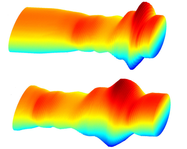
Algorithm 2 allows us to calculate the geodesic between two points in . So, for each point along the geodesic in , one can easily reconstruct the trajectory on using Algorithm 3. Here, one sets as the starting point and as the TSRVF of the trajectory. Fig. 3 shows one example of calculating geodesic using the numerical method in Algorithm 2, where , the set of SPDMs. In this plot, each SPDM matrix is visualized by an ellipsoid and a trajectory on by a sequence of ellipsoids. The left panel shows two original trajectories and (their representations are and ), the end point of the trajectory shot (), and baseline path . In this case, we selected as the starting point and computed the shooting direction such that . The bottom panel shows the evolution of norm between the shot trajectory and the target during the shooting algorithm.
 |
 |
3.4 Geodesic Distance on
Using the natural Riemannian metric on (defined in Eqn. 2), the geodesic distance between the two points is defined as the following.
Definition 2
Given two trajectories , and their representations , and let , be the geodesic between and on , the geodesic distance is given as:
| (4) |
This distance has two components: (1) the length between the starting points on , ; and (2) the standard norm on between the TSRVFs of the two trajectories, where represents the parallel transport of along to . Since we have a numerical approach for approximating the geodesic, this same algorithm can also provide an estimate for the geodesic distance.
3.5 Geodesic Distance on Quotient Space
The main motivation of using TSRVF representation for trajectories on and constructing the distance to compare two trajectories comes from the following. If a trajectory is warped by , resulting in , what is the TSRVF of the time-warped trajectory? The new TSRVF is given by:
Theorem 2
For any two trajectories and their representations , the metric satisfies , for any
Proof: First, if a trajectory is warped by , the resulting trajectory is , and the starting point does not change. If the original representation of is , the resulting representation is . Second, the baseline connecting the starting points of given two trajectories will not change with respect to arbitrary ’s since the starting points are fixed, so for . Starting with the left side, we simplify as follows:
| (5) |
where we have used
Theorem 2 reveals the advantage of using TSRVF representation: the action of on under the metric is by isometries. The isometry property of time-warping action under the metric allows us to compare trajectories in a manner that the comparison is invariant to the time warping. This is achieved through defining a distance in the quotient space of reparameterization group.
To form the quotient space of modulo the re-parameterization group, we first introduce as the set of all non-decreasing, absolutely continuous functions on such that and . This set is a semigroup with the composition operation (it does not have a well-defined inverse). It can be shown that is a dense subset of . Consequently, the orbit of a TSRVF under the action of is exactly the same as the closure of the orbit of under the action of . Since the orbits under form closed sets [16], while those under do not, we choose to work with the former, at least for the formal development. But in practice, we will approximate the theoretical solutions using the elements of . We define the quotient space as the set of all orbits under the action of , with each orbit being:
To understand the orbit, one can view it as an equivalence class. For any two trajectories and their representations in , , we define them to be equivalent when: (1) ; and (2) there exists a sequence such that converges to . In other words, if two trajectories have the same starting point, and the TSRVF of one can be time-warped into the TSRVF of the other, using a sequence of time-warpings, then these two trajectories are deemed equivalent to each other. Theorem 2 indicates that if two trajectories are warped by the same function, the distance between them remains the same. In other word, the orbits in are “parallel” to each other.
Our goal is to define a distance such that it is invariant to the time-warping of trajectories. This can be achieved by comparing trajectories through their equivalence classes (or the orbits). That is, define a metric on the quotient space using the inherent Riemannian metric from . The geodesic distance on is defined as follows.
Definition 3
The geodesic distance on is the shortest distance between two orbits in , given as
| (6) | |||||
The geodesic between and is obtained by forming geodesics between all possible cross pairs in sets and . Since the group action is by isometries, we can fixed one point, say , and search over all that minimizes Eqn. 6.
Next, we focus on the problem of pairwise temporal registration between two trajectories. Eqn. 6 not only defines a metric on the quotient space but also provides an objective function for registering two trajectories: the optimal for Eqn. 6 aligns to . That is the point is optimally matched with the point . To solve Eqn. 6, it is equivalent to optimize the following equation:
| (7) |
where is the geodesic between and , and means parallel transport along to . Note that the time-warping acting on changes the underlying geodesic between two trajectories. Algorithm 4 describes a numerical solution for optimizing Eqn. 7 on a general manifold .
Algorithm 4
Pairwise registration of two trajectories on
Represent two trajectories by their TSRVFs, and . Let , and set (a large integer), and a small .
- 1.
Select one point, say , as the starting point and the other, , as the target point, where denotes , for . In this step, let .
- 2.
Obtain such that and .
- 3.
Parallel transport to the tangent space along , denoted as . Align to using Dynamic Programming Algorithm and obtain the optimal warping function .
- 4.
Update by composition. If or stop. Else, set , and go back to step 3.
Note that Step 2 corresponds to the first argument and Step 3 corresponds to the second argument in Eqn. 7, respectively. The
optimization over the warping function in Step 3 is achieved using the Dynamic Programming Algorithm [24].
Here one samples the interval using discrete points and then restricts to
only piecewise linear ’s that pass through that grid.
In Fig. 4, we present one example of aligning two trajectories and on space of SPDMs.
 |
 |
| Before: and | After: and |
 | |
Fast Approximation: Since pairwise temporal registration algorithm involves multiple evaluations of the exponential map and dynamic programming alignment, it is not computationally efficient. One way to speed up this optimization is to use an approximate method: approximate the baseline connecting two trajectories first (using geodesic between the starting points of trajectories) and then align their TSRVFs. Another way is to find an explicit expression for the exponential map. This seems possible only for a simple manifold, such as , but for a complicated manifold, such as , the analytical expressions are not known. In the experiment section, we use the approximate method to speed up the registration and comparison.
If we compare the proposed framework with that in [16], we see several advantages. The proposed work perseveres the invariance properties achieved in [16], but does not require choosing a reference point. Also, the proposed framework naturally includes the difference between the starting points of two trajectories that are ignored in [16]. Since the velocity vectors here are transported to the starting point of a trajectory, along that trajectory, as opposed to a transport to an arbitrary reference point in [16], this representation is more stable.
3.6 Statistical Summarization of Multiple Trajectories
Since defines a metric in the quotient space , this framework allows us to perform statistical analysis of multiple trajectories in . Given a set of trajectories , we are interested in computing the average of these trajectories and using it as a template for registering these trajectories. This sample average is calculated using the notion of Karcher mean [25]. In the space of , the Karcher mean is defined to be:
Note that is an orbit (equivalence class of trajectories) and one can select any element of this orbit as a template to help to align multiple trajectories.
Algorithm 5
Karcher mean
For each , compute its TSRVF , denote as . Let , be the initial estimate of the Karcher mean (e.g. we can choose one of the trajectories). Set small .
- 1.
- 2.
Compute the average direction: , .
- 3.
If and , stop. Else, update in the direction of using exponential map: , where is the step size. We often let .
- 4.
Set , return to step 2.
After obtaining the converged , one can compute the covariant integral using Algorithm 3, denoted by , which is the Karcher mean of . Fig. 5 shows one result on calculating the mean of given simulated trajectories. The upper panel shows the simulated trajectories. The bottom panel shows mean trajectory in two cases: before alignment and after alignment. One can see that after the alignment, the structure of these trajectories are preserved.
| Simulated trajectories: | |
|---|---|
 |
 |
 |
 |
| Mean before registration | Mean after registration |
4 Video-Based Activities Recognition
Now we turn to evaluation of the framework developed so far on test datasets involving action recognition using videos. While there are several application secures involving video-based action recognition, we try two applications here: (1) hand-gesture recognition, where one classifies the hand motion into pre-determined classes using video data, and (2) visual speech recognition, where one classifies phrases uttered using videos of lip movements.
4.1 Representations of Videos as Trajectories on
The video data is typically extremely high-dimensional, a short video with 50-frames could have more than a million pixel values. To represent a video or a frame in this video, researchers extract few relevant features from the data, forming low-dimensional representations and devise statistical analysis of these features directly. One common technique is to extract a covariance matrix of relevant features to represent each frame in the video [3, 26, 8]. The definition of a covariance feature for a frame is as follows: At each pixel (or patch) of the frame image, extract an -dimension local feature (e.g. pixel location, intensity, spatial derivatives, HOG features, etc), and then calculate a covariance matrix of those local features over the whole frame, i.e. sum over the spatial coordinates. More precisely , let denote a -dimensional feature at location in the image . The empirical estimate of the covariance matrix of is given by: , where is the empirical mean feature vector. The covariance matrix provides a natural way to fuse multiple local features, across the whole image. The dimension of the representation space, , is much smaller than the image size .
A video of human activities is now replaced by a sequence of covariance matrices. Therefore, each video is represented by a parameterized trajectory on the space of , and we can utilize the previous framework to analyze these trajectories. Sometime, as in the hand-gesture recognition, we can localize features better by dividing the image frame into four quadrants and computing a covariance matrix for each quadrant. Then, each frame is represented as an element of , and the whole video as .
4.2 Hand Gesture Recognition
Hand gesture recognition using videos is an important research area since gesture is a natural way of communication and expressing intentions. People use gestures to depict sign language for deaf, convey messages in loud environment and to interface with computers. Therefore, an accurate and automated gesture recognition system would broadly enhance human-computer interaction and enrich our daily lives. In this section, we are interested in applying our framework in video-base (dynamic) hand gesture recognition. We use the Cambridge hand-gesture dataset [7] which has 900 video sequences with nine different hand gestures: 100 video sequences for each gesture. The nine gestures result from 3 primitive hand shapes and 3 primitive motions, and as collected under different illumination conditions. Some example gestures are shown in Fig. 6. The gestures are imaged under five different illuminations, labeled as Set1, Set2, , Set5.
 |
In addition to the illumination variability, the main challenge here comes from the fact that hands in this database are not well aligned, e.g. the proportion of a hand in an image and the location of the hand are different in different video sequences. To reduce these effects we evenly split one image into four quadrants (upper-left, upper-right, bottom-left, bottom-right) with some overlaps. Each of the four quadrants is represented by a sequence of covariance matrices (on the SPDMs manifold ). In this experiment, we use HOG features [27] to form a covariance matrix per image quadrant as follows. We use blocks of pixel cells with histogram channels to form HOG features. Those HOG features are then used to generate covariance matrix for each quadrant of each frame. Thus, our representation of a video is now given by .
Since we have split each hand gesture into four dynamic parts, the total distance between any two hand gestures is a composite of four corresponding distances. For each corresponding dynamic part, e.g. the upper-left part, we first the parts across videos (using Algorithm 4) individually and then compare them using the metric , denoted by . The final distance is obtained using an weighted average of the four parts: and . For each illumination set, we use different weights, and these weights are trained using randomly selected half of the data ( video sequences) in that set, and the other half of the data are used for the testing. Table 1 shows our results using the nearest neighbor classifier on all five sets. One can see that after the alignment, the recognition rate has significant improvement on every set. Also, we have reported the state-of-art results on this database [28, 29]. One can see that our method outperforms these methods.
| Method | Set1 | Set2 | Set3 | Set4 | Set5 | |
|---|---|---|---|---|---|---|
| TCCA [6] | 81% | 81% | 78% | 86 % | - | |
| RLPP [5] | 86% | 86% | 85% | 88 % | - | |
| PM 1-NN [29] | 89% | 86% | 89% | 87 % | - | |
| PMLSR [28] | 93% | 89% | 91% | 94 % | - | |
| Our | before alignment | 94% | 91% | 90% | 88% | 77% |
| after alignment | 99% | 97% | 97% | 96% | 98% | |
| Improvement | 5% | 6% | 7% | 8% | 21% | |
4.3 Visual Speech Recognition
This application is concerned with visual speech recognition (VSR), or lip-reading, using close-up videos of human facial movements. Speech recognition is important because it allows computers to interpret human speech and take appropriate actions. It also has applications in biometric security, human-machine interaction, manufacturing and so on. Speech recognition is performed through multiple modalities - the common speech data consists of both audio and visual components. In the case the audio information is either not available or it is corrupted by noise, it becomes important to understand the speech using the visual data only. This motivates the need for VSR.
The process of visual speech recognition is to understand the words uttered by speakers, derived from the visual cues. Movements of the tongue, lips, jaw and other speech related articulators are involved to make sound. To represent a video of such dynamic process, we extract a covariance matrix for each frame. Now each video becomes a parameterized trajectory on the space of and we can utilize the proposed framework to analysis these trajectories. In the experiments reported here, we utilize the commonly used OuluVS dataset [30] which includes 20 speakers, each uttering 10 everyday greetings five times: Hello, Excuse me, I am sorry, Thank you, Good bye, See you, Nice to meet you, You are welcome, How are you, Have a good time. Thus, totally the database has 1000 videos; all the image sequences are segmented, having the mouth region determined by manually labeled eye positions in each frame [31]. Some examples of the segmented mouth images are shown in Fig. 7.
 |
 |
 |
 |
For each video frame , we extract a covariance matrix representing seven features: . The resulting trajectories in are aligned using Algorithm 4 and compared using distance defined in Eqn. 6. In Fig. 8 (a), we show some optimal ’s obtained to align one video of phrase (“excuse me”) to other videos of the same phrase spoken by the same person. One can see that there exist temporal differences in the original videos and they need to be aligned before further analysis. In (b), we show the histogram of ’s (differences between distances before and after alignment). In this case, each person has videos, and we can calculate pairwise distances before and after alignment, and their differences. For all persons in this dataset, we have such differences. From the histogram of these differences, one can see that after the alignment, the distances (’s) consistently become smaller. Note that one can choose other features to obtain a better representation perhaps, but the main point here is the improvement in temporal alignment and reduced distances between trajectories.
 |
 |
| (a) | (b) Histogram of ’s |
To compare classification performance with previous methods [30, 4], we perform the experiment on a subset of the whole dataset, which contains video sequences by removing some short videos due to the restriction of the method in [30]. (Although our method do not have this restriction, to compare fairly, we perform the experiment in the same subset). Then, we perform the Speaker-Dependent Test (SDT, see [30] for details) on this subset. The recognition rate is calculated based on Nearest Neighbor (NN) classifier. Table 2 shows the average first nearest neighbor (1NN) classification rate of our method and previous methods. One can see that even with a simple classifier, our method has the classification rate of , which is better than [4]’s. This indicates the advantages of proposed intrinsic method compared with the one in [4]. One can also see that, there are percent of improvement after the alignment (registration), which demonstrates the importance of removing temporal difference in comparing of the dynamic systems in computer vision. Several other papers have reported higher classification rates on this dataset by they generally use advanced classier (e.g. SVM, leave-one-out cross valuation), additional information (e.g. audio, image depth) and machine learning techniques [32, 33, 34]. Thus, their results are not directly comparable with our results.
5 Conclusion
In summary, we have proposed metric-based approach for simultaneous alignment and comparisons of trajectories on , the Riemannian manifold of covariance matrices (SPDMs). In order to facilitate our analysis, we impose a Riemannian structure on this manifold, induced by the action of and , resulting in explicit expressions for geometric quantities such as parallel transport and Riemannian curvature tensor. Returning to the trajectories, the basic idea is to represent each trajectory by a starting point and a TSRVF which is a curve in the tangent space . The metric for comparing these elements is a composed of: (a) the length of the path between the starting points and (b) the distortion introduced in parallel translation TSRVFs along that path. The search for optimal path, or a geodesic, is based on a shooting method, that in itself uses geodesic equations for computing the exponential map. Using a numerical implementation of the exponential map, we derive numerical solutions for pairwise alignment of covariance trajectories and to quantify their differences using a rate-invariant distance. We have applied this framework to covariance tracking in video data, with applications to hand-gesture recognition and visual-speech recognition, and obtain state of the art results in each case.
References
- [1] V. Arsigny, P. Fillard, X. Pennec, and N. Ayache, “Log-Euclidean metrics for fast and simple calculus on diffusion tensors,” Magnetic Resonance in Medicine, vol. 56, no. 2, pp. 411–421, August 2006.
- [2] X. Pennec, P. Fillard, and N. Ayache, “A Riemannian framework for tensor computing,” Int. J. Comput. Vision, vol. 66, no. 1, pp. 41–66, 2006.
- [3] O. Tuzel, F. Porikli, and P. Meer, “Region covariance: A fast descriptor for detection and classification,” in 9th European Conference on Computer Vision, 2006, pp. 589–600.
- [4] J. Su, A. Srivastava, F. de Souza, and S. Sarkar, “Rate-invariant analysis of trajectories on Riemannian manifolds with application in visual speech recognition,” in 2014 IEEE Conference on CVPR, June 2014, pp. 620–627.
- [5] M. T. Harandi, C. Sanderson, A. Wiliem, and B. C. Lovell, “Kernel analysis over Riemannian manifolds for visual recognition of actions, pedestrians and textures,” in Proceedings of the 2012 IEEE Workshop on the Applications of Computer Vision, 2012, pp. 433–439.
- [6] T.-K. Kim and R. Cipolla, “Canonical correlation analysis of video volume tensors for action categorization and detection,” IEEE Transactions on Pattern Analysis and Machine Intelligence, vol. 31, no. 8, pp. 1415–1428, Aug 2009.
- [7] T.-K. Kim, K.-Y. K. Wong, and R. Cipolla, “Tensor canonical correlation analysis for action classification,” in IEEE Conference on CVPR, June 2007, pp. 1–8.
- [8] K. Guo, P. Ishwar, and J. Konrad, “Action recognition in video by sparse representation on covariance manifolds of silhouette tunnels,” in Proceedings of the 20th International Conference on Recognizing Patterns in Signals, Speech, Images, and Videos, 2010, pp. 294–305.
- [9] P. E. Jupp and J. T. Kent, “Fitting smooth paths to speherical data,” Journal of the Royal Statistical Society. Series C (Applied Statistics), vol. 36, no. 1, pp. 34–46, 1987.
- [10] R. J. Morris, J. Kent, K. V. Mardia, M. Fidrich, R. G. Aykroyd, and A. Linney, “Analysing growth in faces,” in International conference on Imaging Science, Systems and Technology, 1999.
- [11] A. Kume, I. L. Dryden, and H. Le, “Shape-space smoothing splines for planar landmark data,” Biometrika, vol. 94, pp. 513–528, 2007.
- [12] C. Samir, P.-A. Absil, A. Srivastava, and E. Klassen, “A gradient-descent method for curve fitting on Riemannian manifolds,” Foundations of Computational Mathematics, vol. 12, no. 1, pp. 49–73, 2012.
- [13] J. Su, I. L. Dryden, E. Klassen, H. Le, and A. Srivastava, “Fitting optimal curves to time-indexed, noisy observations on nonlinear manifolds,” Journal of Image and Vision Computing, vol. 30, no. 6-7, pp. 428–442, 2012.
- [14] W. S. Kendall, “Barycenters and hurricane trajectories,” arXIV, vol. 1406.7173, 2014.
- [15] J. O. Ramsay and B. W. Silverman, Functional Data Analysis, ser. Springer Series in Statistics. Springer, June 2005.
- [16] J. Su, S. Kurtek, E. Klassen, and A. Srivastava, “Statistical analysis of trajectories on Riemannian manifolds: Bird migration, hurricane tracking and video surveillance,” The Annals of Applied Statistics, vol. 8, no. 1, pp. 530–552, 03 2014.
- [17] A. Srivastava, E. Klassen, S. Joshi, and I. Jermyn, “Shape analysis of elastic curves in euclidean spaces,” IEEE Transactions on Pattern Analysis and Machine Intelligence, vol. 33, no. 7, pp. 1415–1428, July 2011.
- [18] I. L. Dryden, A. A. Koloydenko, and D. Zhou, “Non-euclidean statistics for covariance matrices with applications to diffusion tensor imaging,” Annals of Applied Statistics, vol. 3, no. 3, p. 1102?1123, 2009.
- [19] J. Jost, Riemannian Geometry and Geometric Analysis. Springer, 2005.
- [20] A. Schwartzman, W. Mascarenhas, and J. Taylor, “Inference for eigenvalues and eigenvectors of gaussian symmetric matrices,” Annals of Statistics, vol. 36, no. 6, pp. 2886–2919, 2008.
- [21] W. Förstner and B. Moonen, “A metric for covariance matrices,” Technical report, Department of Geodesy and and Geoinformatics, Stuttgart University, 1999.
- [22] P. T. Fletcher and S. Joshi, “Principal geodesic analysis on symmetric spaces: Statistics of diffusion tensors,” in ECCV Workshops CVAMIA and MMBIA. Springer-Verlag, 2004, pp. 87–98.
- [23] O. Tuzel, F. Porikli, and P. Meer, “Pedestrian detection via classification on Riemannian manifolds,” IEEE Trans. Pattern Anal. Mach. Intell., vol. 30, no. 10, pp. 1713–1727, Oct. 2008.
- [24] D. P. Bertsekas, Dynamic Programming and Optimal Control. Athena Scientific, 1995.
- [25] H. Karcher, “Riemannian center of mass and mollifier smoothing,” Communications on Pure and Applied Mathematics, vol. 30, no. 5, pp. 509–541, 1977.
- [26] F. Porikli, O. Tuzel, and P. Meer, “Covariance tracking using model update based on lie algebra,” in IEEE Conference on CVPR, Washington, DC, USA, 2006, pp. 728–735.
- [27] N. Dalal and B. Triggs, “Histograms of oriented gradients for human detection,” in International Conference on CVPR, vol. 2, June 2005, pp. 886–893.
- [28] Y. M. Lui, “Human gesture recognition on product manifolds,” Journal of Machine Learning Research, vol. 13, no. 1, pp. 3297–3321, 2012.
- [29] Y. M. Lui, J. Beveridge, and M. Kirby, “Action classification on product manifolds,” in IEEE Conference on CVPR, June 2010, pp. 833–839.
- [30] G. Zhao, M. Barnard, and M. Pietikäinen, “Lipreading with local spatiotemporal descriptors,” IEEE Transactions on Multimedia, vol. 11, no. 7, pp. 1254–1265, 2009.
- [31] G. Zhao, M. Pietikäinen, and A. Hadid, “Local spatiotemporal descriptors for visual recognition of spoken phrases,” in Proceedings of the International Workshop on Human-centered Multimedia, ser. HCM ’07, 2007, pp. 57–66.
- [32] Y. Pei, T.-K. Kim, and H. Zha, “Unsupervised random forest manifold alignment for lipreading,” in Proceedings of 2013 IEEE ICCV, Washington, DC, USA, 2013, pp. 129–136.
- [33] Z. Zhou, G. Zhao, and M. Pietikainen, “Towards a practical lipreading system,” in Computer Vision and Pattern Recognition (CVPR), 2011 IEEE Conference on, June 2011, pp. 137–144.
- [34] Z. Zhou, G. Zhao, and M. Pietikainen, “Lipreading: A graph embedding approach,” in Pattern Recognition (ICPR), 2010 20th International Conference on, Aug 2010, pp. 523–526.
- [35] E. Andruchow, G. Larotonda, L. Recht, and A. Varela, “The left invariant metric in the general linear group,” arXiv, vol. 1109.0520, 2011.
Appendix A Riemannian Structure on and Its Quotient Space
We start with , the set of all with unit determinant. For the identity matrix , the tangent space at identity is given by , the space of all matrices with trace zeros. The tangent space at any other point , , is given by . Each left-invariant vector field on is determined by its value at : , where and . Note that any group naturally acts on itself and we will use this fact for .
The lie algebra can be expressed as the direct sum of two vector subspaces: ,
where , and .
The tangent space at any arbitrary point also has a similar decomposition:
for any , we have such that and
.
Riemannian metric on : Now we define the Riemannian metric on that will later be used for inducing a Riemannian structure on . For , we define a metric as . At any other point , the metric is calculated by pulling back the tangent vectors to , by multiplying on the left, i.e. . Thus, the inner product (or the Riemannian metric) is given by:
| (8) |
where . This pullback operation ensures that this
metric is invariant to the left action of , i.e. . In fact, the difference
in this framework to the Riemannian metric used in [2] comes from the mapping used for pullback.
The mapping used in that paper is not left invariant.
Geodesic paths on : An important consequence of the -invariance (Eqn. 8) is that we can simplify some calculations by transforming our problems appropriately. For instance, if we need to compute a geodesic between two arbitrary elements , then we can first solve the problem of computing the geodesic, between and , where , and then multiply on the left by . The geodesic between and is given by , according to [35], where , and indicates the Frobenius norm. In fact, if is symmetric and positive definite, then and the geodesic has the simple expression , so that the desired geodesic between and is . The geodesic distance between the two points is given by:
| (9) |
Riemannian curvature tensor on : Let , and be three tangent vectors at a point , and we want to compute the Riemannian curvature tensor . While the general form for is complicated [35], if , and where and are elements of , then the tensor is given by:
where . (This use of square brackets is called Lie bracket and should be distinguished from the use of square brackets to denote equivalence classes.)
Now we consider a quotient space of and, using the theory of Riemannian submersion, inherit some of these formulas to this quotient space. Define the right action of on according to:
An orbit under this action is given by . The set of these orbits forms the quotient space . Since is a closed subgroup of , the quotient space is a manifold.
Using the Riemannian metric on , it is easy to specify the tangent bundle of the quotient space. The tangent space is simply the subspace of which is orthogonal , the space tangent to the orbit at . It is well known that . The subspace of which is orthogonal to is . So, we have . For any arbitrary , the vector space tangent to the quotient space at , can be identified with the set .
Riemannian metric on : Now that we have the tangent bundle of the quotient space, we can define a Riemannian metric on this quotient space by inducing it from the larger space . This is possible since the action of is by isometries under that metric (and the fact that is a closed set). By isometry we mean that , for any and . Therefore, we can induce this metric from to the quotient space . For any two vectors , with the above identification, we define the metric as: , for any . Note that .
Geodesic paths on : The geodesics in the quotient space can be expressed using those geodesics in the larger space, , that are perpendicular to every orbit they meet. Therefore, a geodesic between the points and in is given by , where such that . The last part means that there exists an such that . The geodesic distance between the two orbits is given by:
| (10) |
Parallel transport of tangent vectors along geodesics on : Let be a tangent vector that needs to be translated along a geodesic path given by , where . Let such that is identified with , where . Then, the parallel transport of along the geodesic is identified with the vector field along on .
Riemannian curvature tensor on : Let , and be three tangent vectors at a point , and we want to compute the Riemannian curvature tensor on the quotient space. Let , and be elements of such that , and , where one can use any for this purpose. Then, the tensor is given by:
where as earlier.