Ab initio holography
Abstract
We apply the quantum renormalization group to construct a holographic dual for the U(N) vector model for complex bosons defined on a lattice. The bulk geometry becomes dynamical as the hopping amplitudes which determine connectivity of space are promoted to quantum variables. In the large limit, the full bulk equations of motion for the dynamical hopping fields are numerically solved for finite systems. From finite size scaling, we show that different phases exhibit distinct geometric features in the bulk. In the insulating phase, the space gets fragmented into isolated islands deep inside the bulk, exhibiting ultra-locality. In the superfluid phase, the bulk exhibits a horizon beyond which the geometry becomes non-local. Right at the horizon, the hopping fields decay with a universal power-law in coordinate distance between sites, while they decay in slower power-laws with continuously varying exponents inside the horizon. At the critical point, the bulk exhibits a local geometry whose characteristic length scale diverges asymptotically in the IR limit.
I Introduction
According to the AdS/CFT correspondence[1, 2, 3], quantum field theories are dual to gravitational theories in a spacetime with one higher dimension. The extra dimension in the bulk can be interpreted as a length scale in the renormalization group (RG) flow[4, 5, 6, 7, 8]. However, the flow generated along the extra dimension in holography is different from the conventional RG flow because the bulk theories are in general quantum theories. In order to make the connection between RG and holography precise, one has to introduce quantum RG (QRG)[9, 10, 11]. According to QRG, general -dimensional quantum field theories are equivalent to -dimensional theories that include quantum gravity, provided that the quantum field theories can be regularized covariantly in curved spacetime[10, 11].
Conventional renormalization group describes the flow of the couplings (sources) generated by coarse graining defined in the space of all sources allowed by symmetry. In QRG, only a subset of the sources is included. The sources in the subset are promoted to quantum mechanical operators, and a quantum Hamiltonian governs the evolution of the dynamical sources under scale transformations. Quantum fluctuations in the RG flow precisely capture the effect of other couplings that are not explicitly included. In the bulk, this amounts to the fact that composite operators are generated after lowering the position of the UV boundary by integrating out bulk degrees of freedom[7, 8]. Intuitively, sources become quantum mechanical because high-energy modes act as fluctuating sources from the point of view of low-energy modes[9, 10, 11, 12].
Despite the formal mapping between general quantum field theories and gravitational theories, classical and local geometries are expected to arise only for a special set of quantum field theories[13, 14, 15]. In the presence of a large number of degrees of freedom, the quantum fluctuations of the RG flow become weak, which allows one to use a classical description. However, it is much more non-trivial to have locality in the bulk. Generally, there exist infinitely many non-local operators, and locality arises only when the sources for the non-local operators are suppressed. In QRG, the condition for the emergence of local geometry translates into stringent constraints on the beta functions of the quantum field theory[16, 17]. From the constraints, one can try to find quantum field theories that exhibit a local geometry in the bulk. On the other hand, one can use varying degrees of locality that emerge in the bulk as a diagnostic that differentiates one phase from another. The bulk locality serves as a useful order parameter for characterizing phases of matter using geometry, which is one of the primary goals of applying holography to condensed matter systems[18, 19, 20, 21].
In this paper, we apply QRG to a three-dimensional U(N) vector model regularized on a Euclidean lattice, which can be viewed as a quantum Bose-Hubbard model of components in two space dimensions and an imaginary time. It supports an interacting field theory at the critical point between the insulating (gapped) phase and the superfluid (long-range ordered) phase. The full bulk equations of motion derived from QRG are solved in the large limit on finite size lattices. From a finite size scaling analysis, we show that different phases indeed exhibit different degrees of bulk (non-) locality in the thermodynamic limit.
Here is the outline of the paper. In Sec. II, we start with the U(N) vector model for complex bosons defined on a -dimensional lattice. In this model, the general single-trace operators can be written as , where is a complex boson with flavour defined at site . The single-trace operators involve only one flavour contraction and are bi-local in space[22, 23, 24]. The set of single-trace operators has a special status in that all other singlet operators can be constructed as composites of single-trace operators. They describe the kinetic term that connects pairs of sites through hopping. In the vector model, all single-trace operators are quadratic, and it is not enough to include only single-trace operators to describe the phase transition from the insulating (gapped) phase to the superfluid (symmetry-broken) phase. Therefore, we also include a quartic double-trace operator. We treat the single-trace hopping terms as deformations to the on-site action that includes the single-trace mass term and the double-trace interaction term. In the conventional RG, a series of coarse graining generates an infinite tower of multi-trace operators[25]. In QRG, one only keeps track of single-trace deformations at the expense of promoting the sources for the single-trace operators to quantum variables. We derive a -dimensional bulk action whose degrees of freedom are scale dependent bi-local hopping fields and their conjugate variables , where is the logarithmic length scale. The bulk theory describes the quantum mechanical RG flow in the space of single-trace operators. In the large limit, the path integral in the bulk can be replaced by saddle point equations whose solution determines the classical geometry in the bulk. In Sec. III A, an analytic solution to the bulk equations of motion is found in the deep insulating phase by treating hoppings as small perturbations compared to the on-site terms. Away from the deep insulating phase, we resort to numerical solutions. Sec. III B and C outline the numerical scheme. In Sec. IV, the numerical solutions obtained for three dimensional lattices with linear sizes are presented. Then we extract the behaviour of the solution in the thermodynamic limit from finite size scaling.

Fig. 1, which is the key result of the paper, summarizes the numerical solution in the thermodynamic limit, which is suggested from the finite size scaling analysis. Here represents the on-site mass term, which tunes the system away from the critical point either to the insulating phase () or to the superfluid phase () depending on its sign. Although only the nearest neighbor hoppings are turned on at the UV boundary at , further neighbor hoppings are generated inside the bulk with . In the insulating phase, the hopping fields decay exponentially not only in but also in . As a result, the lattice is fragmented into decoupled sites in the large limit. While the scale beyond which fragmentation occurs remains small in the deep insulating phase, it diverges as the critical point is approached in the thermodynamic limit. In the superfluid phase, on the other hand, a new scale emerges. Instead of fragmentation, the system loses locality beyond a critical scale , which is called the horizon. At the horizon, the hopping fields decay in a universal power-law in . Inside the horizon with , the hopping fields decay with a slower power-law with continuously varying exponents. The horizon scale diverges as the critical point is approached from the superfluid side. At the critical point, the bulk exhibits a local geometry with a characteristic length scale that remains finite for finite and diverges only in the IR limit. In summary, the insulating phase, the superfluid phase and the critical point exhibit ultra-local, non-local and local bulk geometries, respectively. In this sense, locality serves as a holographic order parameter that characterizes different phases of matter. The goal of Sec. IV is to justify the holographic phase diagram in Fig. 1. For related works on the holographic description of the vector models, see Refs. [22, 23, 26, 25, 27, 28, 29, 24].
II Holographic action for vector model on a lattice
We consider a bosonic vector model in -dimensional Euclidean space,
| (1) |
where refers to the complex boson field with flavours, , is the mass of the bosons, and is the quartic coupling. We regularize the continuum theory on a -dimensional hypercubic lattice,
| (2) |
where
| (3) | |||||
| (4) |
Here run over the -dimensional Euclidean lattice for the component bosonic fields with . represents on-site terms, and includes the hopping term and general quartic interactions. To guarantee the action is real, we impose and . Here we consider the case where is real. We could make complex by turning on a background gauge field. The background gauge field in general breaks the time-reversal symmetry, if we go to Minkowski space by Wick-rotating one of the Euclidean directions into real time. For general and , the model has the symmetry. The symmetry is enhanced to when ’s are real and . The action is proportional to in the large limit with fixed , , and .
There is a redundancy in the parameters of the action, and the action is invariant under
| (5) |
By shifting and , could have been entirely absorbed into . Here is explicitly singled out because we will use as ‘the reference theory’ and treat as a deformation. In other words, the renormalization group (RG) flow will be defined in terms of the flow of the parameters in which is defined with respect to the fixed with . It is emphasized that one can describe not only the insulating (gapped) phase but also the superfluid (symmetry broken) phase because can be arbitrarily large to support a Mexican hat potential for . The freedom to choose different and amounts to choosing different RG schemes, which does not affect physical observables.
We derive a holographic theory for the lattice action in Eq. (2) using the QRG scheme. We start by writing the partition function:
where the measure is given by , and is the number of sites in the lattice. The first step is to remove multi-trace operators in by promoting the sources for the single-trace operators into dynamical variables. Using the representation of the Dirac-Delta function[9]
| (6) |
we introduce a pair of complex conjugate link fields, and for every ordered pair of sites to rewrite the partition function as
where with running over all sites and
| (7) |
with
| (8) |
Here and henceforth, multiplicative constants in the partition function are ignored. In the new action, only single-trace deformations are present. Although the double-trace operator in could have been removed as well, we need to keep the on-site double-trace operator to make sure that the path integral for is well defined for any values of fluctuating sources . The presence of the double-trace operator is also important because it makes the hopping fields genuinely dynamical variables.


Note that is coupled to dynamical sources which connect all possible sites. Therefore the new action is defined on a globally connected network rather than a fixed lattice. The globally coupled network with dynamical hoppings does not have a fixed lattice structure, and should be regarded as indices for ‘events’ rather than fixed coordinates. Since there is no fixed lattice, there is a freedom to relabel each event differently, which corresponds to a discrete local coordinate transformation. So we perform a discrete coordinate transformation,
| (9) |
where site is displaced by a site-dependent D-dimensional shift vector, [26, 10, 11]. Since the full set of events must map to itself, the transformation should form cyclic permutations of the events. This is illustrated in Figs. 2(a),(b). After the local coordinate transformation, is manifestly invariant and the hopping term is transformed to
| (10) |
where the shifted hopping field is given by
| (11) |
The point is that the change introduced by the local coordinate transformation can be compensated by a transformation of the hopping fields because is dynamical. Therefore, the dynamical hopping fields play the role of a dynamical metric in the continuum limit, which guarantees invariance under a set of -dimensional local coordinate transformations in the continuum limit. The set of permutations generated by the shift includes -dimensional local coordinate transformations, which don’t necessarily preserve the coordinate volume locally. An example is given in Fig. 2(c). The fact that the hopping fields play the role of a metric is expected because the physical distance between two sites is determined from the strength of the hopping between them: the larger the hopping between two sites, the shorter the physical distance.
Now we generate RG flow by coarse graining the system in real space. The original field is split up into high- and low- energy fields, where the low-energy field has a mass slightly larger than . The missing fluctuations are carried away by the very massive high-energy fields. Then, the high-energy modes are integrated out to generate quantum corrections for the low-energy modes[30, 31]. For this, we introduce an auxiliary field with an arbitrary mass ,
where
Now we rotate the physical field and the auxiliary field into high- and low-energy fields,
| (12) |
with , and . is the ‘lapse’, which is a site-dependent constant that controls the local speed of coarse graining[32, 10, 11]. Here is the low-energy mode with mass , which is larger than by an infinitesimal amount , and is the high-energy mode with a large mass . After rescaling the fields and renaming , we rewrite the partition function as
where
| (13) |
Integrating out the high energy mode , we obtain the renormalized action for the low energy mode,
| (14) |
where quantum corrections are kept only to the linear order (see Appendix A for details). In the renormalized action, multi-trace operators have been generated for the low energy field. Under the conventional (classical) Wilsonian RG procedure, one would apply the same coarse graining procedure to Eq. (14) to generate even higher-trace deformations. In QRG, we remove the multi-trace deformations before repeating the coarse graining. This way, one can keep only single-trace deformations at each step of coarse graining by making the sources for the single-trace deformations fluctuating. Just as before, we introduce new link fields and to remove the multi-trace deformations,
where
| (15) |
Now we can repeat the coarse graining procedure as before. The coordinates of the ’s can be shifted by a new set of discrete translations, . Then is split into low-energy and high-energy modes where the low energy mode at site has a mass . After rescaling the fields, we integrating out the high energy modes to generate quantum corrections which include multi-trace operators for the low energy fields. We introduce another set of auxiliary fields and to remove the multi-trace operators. From here the pattern is clear. After doing this times, the partition function is written as
where
| (16) |
with . Here , are the dynamical sources and their conjugate variables introduced at the -th step of coarse graining. The site-dependent lapse and shift are chosen independently at each step of coarse graining. Finally, we take the continuum limit in the RG direction by introducing in the limit with fixed . In the limit where is continuous, , , , become , , , . The partition function is written in terms of the path integral for the scale dependent hopping fields and their conjugate fields,
| (17) |
Here , defined in Eq. (8), is the UV boundary action for the dynamical source at . is the bulk action,
| (18) |
with . is an action,
| (19) |
which is defined at the IR boundary . is the scale at which we stop the coarse graining procedure, which can be taken to be infinite.

The new action is written in terms of the fields and which are bi-local within the original -dimensional lattice and local in the direction. If one interprets as ‘time’, the action describes a system of bi-local hopping fields under a Hamiltonian evolution in imaginary time. and correspond to annihilation and creation operators respectively[9], and the last term in Eq. (18) describes the process where two hoppings merge to become a longer-range hopping. This is illustrated in Fig. 3. In the path integral language, all RG paths are summed over for the single-trace operators. The weight for each RG path is determined by the bulk action, .
In the bulk, the lapse and shift vector parameterize local coordinate transformations. The partition function does not depend on because different choices of lapse and shift merely correspond to different renormalization group schemes [10, 11]. As a result, the local coordinate transformation in the bulk is a gauge symmetry. Unlike in the continuum, the action contains terms that are non-linear in the shift. This is because the discrete shift is a finite transformation. When vary slowly in , one can take a continuum limit along the -dimensional directions by writing
| (20) |
where , in the limit that the lattice spacing is small. Then, the shift can be performed infinitesimally, , and one can drop the terms that are non-linear in . In this case, the action is linear in and , which generate -dimensional coordinate transformations in the bulk. Also, in the continuum, the bi-local fields can be represented by an infinite set of fields with arbitrarily large spin. Here we don’t take the continuum limit and proceed with the lattice action.
In the absence of the quartic term (), the theory has a larger symmetry generated by[28, 29]
where is a unitary matrix in the space of all sites in the lattice. The enlarged symmetry is the source of the higher spin gauge symmetry for the free theory with . In the interacting theory with , the symmetry is broken down to the local coordinate transformation. One might keep the higher spin symmetry in the bulk action even when by absorbing the quartic term into the UV boundary action . In that case, there is no in the bulk, and the quartic term is implemented only through the alternative boundary condition determined by [33]. However, this can be done only in the strict large limit where the fluctuations of the dynamical hopping field induced by are negligible. What is less satisfying in this description for the interacting theory is the fact that corrections are singular because the path integral for is ill-defined without the quartic term in for fluctuating hopping fields. Therefore we choose to include the quartic term in the bulk for general , which breaks the higher spin symmetry.
Because the fields are singlets under rotations, the action in Eq. (17) is proportional to in the large limit. Therefore, the partition function can be obtained by the saddle point approximation in the large limit. To that effect, all we need to solve are the equations of motion, which we focus on from now on. Although and are complex conjugates of each other in Eq. (17), their saddle points configurations do not have to satisfy that condition. This is because the amplitude and phase of can take complex values at the saddle point. Therefore, we treat and as independent complex fields in the saddle point equation.
In the gauge with and , the equations of motion for the bulk fields are given by
| (21) |
subject to two boundary conditions
| (22) | ||||
| (23) |
which are derived by extremizing the boundary actions at and , respectively. In the equations of motion, sub-leading terms are dropped in the large limit. From the IR boundary action, one can readily write the IR boundary condition as
| (24) |
where denotes the expectation value of evaluated with respect to at . This relationship must hold anywhere inside the bulk, since the RG process can be stopped at any point. Therefore, the on-shell value of coincides with the 2-point correlation functions at scale , which are completely determined by .
In the end, one has to solve the first order differential equations for and with one set of boundary conditions imposed at the UV boundary and the other imposed at the IR boundary. It is the IR boundary condition that imposes the constraints that the expectation values of operators () have to satisfy for a given set of sources (). In particular, the vacuum expectation value has to satisfy the Ward identity associated with the discrete coordinate transformation,
| (25) |
where is defined in Eq. (11). Since this equation has to be satisfied at all , it becomes a dynamical constraint, , which is the discrete version of the energy-momentum conservation imposed by . This condition is automatically implied by the IR boundary condition even in the fixed gauge with . It is noted that cannot be arbitrary at the IR boundary, but it has to be the actual vacuum expectation value computed from the IR boundary action, .
III Solutions to saddle point equations
In this section, we examine the solution to the equations of motion both analytically and numerically. We assume that translational symmetry is present, in which case and depend only on . Also, since we are maintaining the full and -dimensional inversion symmetries at each scale , all and are real. We focus on the three dimensional cubic lattice of linear size with periodic boundary conditions.
To uniquely determine the solutions we need to impose the boundary conditions in Eqs. (22) and (24). At the UV boundary, Eq. (22) imposes the Dirichlet boundary condition for in the absence of . To impose the IR boundary condition in Eq. (24) we compute by introducing a Hubbard-Stratonovich field which satisfies the saddle-point equation in the large limit (see Appendix B),
| (26) |
where . Then the IR boundary condition becomes
| (27) |
III.1 Analytic solutions in the deep insulating phase
For and , the quadratic on-site action dominates. All correlation functions decay exponentially, resulting in the insulating phase. In this case, one can easily obtain an analytic solution to the equations of motion as a perturbation series in and . To order , the solutions are
| (28) | ||||
| (29) |
Both and decay exponentially as one moves towards the IR boundary. This is expected since bosons are localized at low energies. It is noted that for decays as with increasing . This feature holds generally even when is not small. This is due to the fact that the transformation in Eq. (12) followed by the rescaling by implies up to the contribution from the auxiliary field introduced at each step of coarse graining which has zero correlation length. This implies that
| (30) |
for .
In the insulating phase a large simplification can be made for the IR boundary condition. Since both and decay exponentially in except for , we can approximate them as and for a sufficiently large . In this case, the IR boundary condition reduces to a single-site problem,
| (31) |
where is given by , which is the solution of the on-site saddle point equation .
III.2 Numerical solutions
Since it is hard to solve the full equations of motion analytically in general, we resort to numerical solutions for the superfluid phase and the critical point. We solve the coupled differential equations using a spectral method. The details of the numerical method can be found in Appendix C. Numerical solutions are obtained for the cubic lattice with linear sizes . We set , , and except for the on-site and nearest neighbor hoppings. The nearest neighbor hoppings are set to be , and the on-site ‘hopping’ is tuned to change the physical bare mass,
| (32) |
to drive the phase transition from the insulating phase to the superfluid phase. The physical mass can be either positive or negative whereas the mass of the reference action in Eq. (3) is fixed to be positive. The reason for choosing a positive is to make sure that only short-distance modes are integrated out in the coarse graining procedure.
Although there is no genuine symmetry breaking phase transition in finite systems, features of the superfluid phase and the critical point can be still identified from the behaviors at intermediate length scales before the finite size effect takes over. Henceforth, we will keep using the terminology “superfluid” to refer to systems in parameter regimes which become real symmetry broken states in the thermodynamic limit. Although only the nearest neighbor hopping is turned on at the UV boundary, all further neighbor hoppings are generated inside the bulk. From now on, we will use the notation , to denote the specific fields with in units of the lattice spacing. For example, the three nearest neighbor hopping fields are represented by , , .
III.3 Universal IR boundary condition in finite systems


In Figs. 4 and 5, we plot and for with . For each , we display multiple curves at that cover from the deep insulating phase to the deep superfluid phase across the critical point, which is at in the thermodynamic limit. Since the curves look very similar away from critical point and they start to change rapidly only in its vicinity, we choose the spacing of to be smaller near the critical point and larger away from it. Here, we notice something interesting. No matter what the values of are, all and with approach zero in the large limit. In other words, the system flows to the on-site problem in the deep IR not only in the insulating phase but also in the deep superfluid state. The universal insulating (on-site) behavior in the deep IR limit is due to the finite size effect. For , increases with increasing for small , which is consistent with the expected RG flow in the superfluid phase where the hopping terms become more important at larger length scales. However, the RG length scale eventually becomes greater than the system size. Then the finite size effect becomes important, and the system “flows” back to the insulating behavior in the deep IR. This has to do with the fact that all phases are adiabatically connected to the insulating phase in finite systems.
At first, the finite size effect appears to be detrimental to our goal of characterizing different phases of matter in terms of different IR geometries. However, one can still study the superfluid phase and the critical point by focusing on the behavior of in the intermediate range of before the finite size effect becomes dominant. Moreover, we can use the finite size effect to our advantage. The universal insulating behavior in the IR limit allows us to use the single-site IR boundary condition in Eq. (31), which is much simpler than the full IR boundary condition in Eq. (27). This has a significant implication. A practical difficulty in applying QRG to strongly coupled field theories is that one has to impose the IR boundary condition dynamically. This is done either by extremizing the bulk action in the limit or imposing Eq. (24) at a finite . If one uses the latter scheme, one has to know . Although this does not pose any problem for the present vector model which is exactly solvable in the large limit, this is in general a difficult task for strongly coupled theories (such as matrix models). However, if one can always impose the insulating boundary condition for finite systems one only needs to know the solution to the on-site problem, which is much easier. This allows one to find solutions for finite systems without knowing the IR behavior of the infinite system a priori. Then, one can extract the behaviors in the thermodynamic limit through finite size scaling. This is the strategy we will employ in the rest of the paper.
In order to guarantee that systems with finite sizes flow to the insulating phase, one has to choose to be sufficiently large. The smaller is, and the larger is, has to be larger to ensure that the system flows to the deep insulating state driven by the finite size effect at the IR boundary. This is because it takes longer RG ‘time’ before the finite size effect takes over in deeper superfluid phases and larger lattices. We observed that for all values of we took within the range and all lattice sizes , is sufficient. For larger , it is expected that should grow logarithmically in because corresponds to a logarithmic length scale. Although computational cost increases with increasing , it is still much cheaper to use the on-site boundary condition with a logarithmically larger than using the full boundary condition whose computational cost increases much faster. In Appendix D, we show that the solutions obtained from the on-site boundary condition are indeed identical to the ones obtained with the full boundary condition. From now on, we will use the on-site boundary condition which allows us to obtain full numerical solutions for larger lattices. The plots of the hopping fields for larger lattices can be found in Appendix D.
IV Analysis
In this section, we present the main results of the paper. We first establish the presence of the critical point that divides the insulating phase and the superfluid phase based on the correlation functions measured at the UV boundary. Then we examine how different phases exhibit distinct geometric features in the bulk.
IV.1 UV Boundary

The correlation functions, are given by , which are measured at the UV boundary. In the thermodynamic limit, is the order parameter for the phase transition between the insulating (symmetric) phase and the superfluid (symmetry broken) phase. Although there is no real phase transition in finite lattices, there exists a rather sharp crossover which becomes the phase transition in the thermodynamic limit. To identify the ‘would-be’ phase transition in finite systems, we plot for the largest possible as a function of for in Fig. 6. Although it is not strictly zero even in the insulating phase due to finite size effect, there is a sharp crossover around . The critical point in the thermodynamic limit is at (see Appendix E). From now on, we will use the notation
| (33) |
to denote the deviation of the mass away from the thermodynamic critical point.

In Fig. 7 we plot the full correlation functions as functions of for various values of . In the insulating phase, the correlation functions decay exponentially as expected. The correlation length tends to diverge as the critical point is approached, as is shown in Fig. 7 (a). In the superfluid phase, the correlation functions approach non-zero values in the large distance limit, exhibiting a long range order. As the critical point is approached from the superfluid side, the long range order disappears continuously as is shown in Fig. 7 (b).


At the critical point, we expect that the correlation function decays in a power-law,
| (34) |
with for . In Fig. 8 (a), the correlation function is shown at . The curvature in the log-log plot indicates that the correlation function actually decays slower than an algebraic decay. This is due to the finite size effect which overestimates the correlations due to the periodic boundary condition. The finite size effect effectively pushes the system at to the superfluid side at finite . As will be shown in Sec. IV B. 3, the correlation function decays algebraically at a positive value of that goes to zero only in the infinite limit. To take this into account, we include a constant piece and fit the correlation function with
| (35) |
as is shown in Fig. 8 (b). In the thermodynamic limit, the exponent approaches and tends to vanish as is shown in Figs. 8 (c) and (d). We expect that the error in the critical exponent can be made smaller by increasing the number of basis points that are included to parameterize the radial profile of and in the numerical calculation. For details, see Appendix C.
IV.2 Bulk
Now we set out to understand the different phases from the behaviors of the bulk fields in the -dimensional space.
IV.2.1 Insulating phase


In Fig. 9, the scale dependent hopping fields are plotted in a deep insulating state at for . Although all further neighbor hoppings are generated in the bulk, they remain exponentially small in at all . Furthermore, all hopping fields decay exponentially in in the IR region. Due to the exponential decay both in and , is significant only for small and . As the connectivity of space becomes weaker with increasing , the correlation functions become smaller as is shown in Fig. 10. As increases, the overall magnitude of decreases exponentially while the rate of decay in is unchanged. In the large limit, the space completely loses its connectivity, and gets fragmented into isolated islands. In the RG language, the IR fixed point is described by the decoupled sites. One can quantify the scale of fragmentation in terms of the susceptibility
| (36) |
which is proportional to in the insulating phase, where is the correlation length. As increases, the susceptibility decreases because the hopping amplitudes become smaller in the bulk. In the large limit, saturates to the value determined by the on-site mass term. This is shown in Fig. 11. Although fragmentation is not a sharp transition, we can choose a convenient criterion for definiteness: we define the fragmentation scale to be the scale at which is maximal. It represents a scale around which a crossover occurs from a connected lattice to fragmented space. In Fig. 11, is indicated in the insulating phase, which shows that increases with decreasing , as expected. Fragmentation occurs at longer distance scales when the system is closer to the critical point. The background color in Fig. 12 represents the value of the susceptibility in the bulk for different values of . The curve denoted by represents the fragmentation scale. The curve and other features in the superfluid phase () of Fig. 12 will be discussed in the following section.

Near the critical point, the fragmentation scale can be used to extract the critical exponent , which dictates how the correlation length depends on the distance to the critical point, . The susceptibility is given by at the UV boundary. Inside the bulk, it falls off exponentially in as because of Eq. (30) before saturating to a fixed value of . Therefore, the fragmentation scale is given by . In Fig. 13 we show as a function of , which shows , the expected value for the interacting model we are studying in the large limit. Therefore the fragmentation scale should behave as in the thermodynamic limit.
IV.2.2 Superfluid phase


In Fig. 14, we display the hopping fields inside the superfluid phase at for . Near the UV boundary, decays exponentially in as is the case in the insulating phase. This has to be true even in the superfluid phase because only nearest neighbor hoppings are turned on at the UV boundary, and further neighbor hoppings are generated gradually in the bulk. The exponential decay of the hopping fields is well captured by
| (37) |
with near the UV boundary as is shown in Fig. 15. However, the rate of the exponential decay, becomes smaller as increases, and vanishes at a critical scale . This is shown in Fig. 15.


For , the hopping fields no longer decay exponentially but decay algebraically with a constant off-set,
| (38) |
where the constant off-set turns on continuously as
| (39) |
with an exponent for . After the off-set is subtracted out the hopping fields exhibit pure power-law decays as is shown in Fig. 16. The dependence of the off-set near is displayed in Fig. 16.


The scale represents a ‘horizon’ at and beyond which the system loses locality as sites are connected with each other through non-local hoppings. As a result, the ‘coordinate distance’ is no longer a good measure of the ‘physical distance’ that dictates the actual correlations. Because of the non-local hopping, the physical distance between two sites effectively shrinks to zero. If we were studying a system with a finite temperature with a compact Euclidean time direction in such a way that its length would remain finite as , we would first observe this loss of locality only in the Euclidean time direction. In that case, corresponds to the usual horizon at which only the thermal circle shrinks to zero. In the present case, the limit corresponds to the zero temperature limit, where all directions are equivalent. As a result, the size of space shrinks to zero in all directions at the horizon. It will be interesting to understand what this generalized horizon corresponds to in Minkowski space.
If the off-set was indeed nonzero in the thermodynamic limit, it would imply that any two sites remain coupled with a non-vanishing hopping no matter how far they are. However, Fig. 17 shows that systematically decreases as the system size increases. In order to understand the behavior of in the thermodynamic limit, we need to do a finite size scaling analysis. Fig. 17 shows that the maximum value of at fixed decays as with for as the system size increases. This implies that goes to zero, and the hopping fields decay in a purely algebraic manner for in the thermodynamic limit.


Although the off-set vanishes in the thermodynamic limit, the location of the horizon remains finite, as is shown in Fig. 18. In the deep superfluid phase, is more or less independent of , but sharply increases as the critical point is approached from the superfluid side. This is displayed in Fig. 12. For , the horizon scale diverges at , and the horizon no longer exists for . From the location of the horizon in the bulk, we define to be the critical mass for finite lattices, e.g., . Although the critical point is at in the thermodynamic limit, is different from zero for finite due to the finite size effect. A finite size scaling in Fig. 18 suggests that indeed goes to zero in the thermodynamic limit.


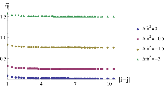
In the absence of the off-set in the thermodynamic limit, what distinguishes the horizon at from the region inside the horizon with is the exponent with which the hopping fields decay. Fig. 19 shows that inside the horizon is smaller than defined at the horizon. The exponent tends to approach nonzero values for all z in the thermodynamic limit as is shown in Fig. 19.

Remarkably, the exponent at the horizon is independent of as is shown in Fig. 20. This suggests that the horizon is characterized by a universal exponent associated with the decay of the hopping fields. The location where the decay of the hopping fields exhibits the universal exponent precisely coincides with the location where turns on and vanishes in finite lattices. It is interesting to note that the hopping fields exhibit universal ‘critical behavior’ that is akin to a continuous phase transition. This should not be confused with the usual phase transition where the correlation length diverges as is tuned from the insulating phase to the superfluid phase. The ‘transition’ that happens at is associated with the divergence of the length scale for the renormalized hopping fields within the superfluid phase.
As the ‘short-distance’ modes are integrated out, the effective action is renormalized by further neighbor hoppings. In the insulating phase, the further neighbor hopping fields remain exponentially small, and the renormalized action remains local at all scales. In the superfluid phase, the system can not keep the locality as further neighbor hoppings are proliferated beyond the critical scale . The presence/absence of the horizon can be used as a ‘holographic order parameter’ that distinguishes the superfluid/insulating phases.
The non-locality in the bulk could have been avoided if one had allowed for spontaneous symmetry breaking by turning on an infinitesimally small symmetry breaking field before taking the thermodynamic limit. In that description, one starts with a new vacuum with broken symmetry, and fluctuations around the new vacuum are described by the Goldstone modes. Here the spontaneous symmetry breaking is not allowed because the large volume limit is taken in the absence of the symmetry breaking field. The emergence of the non-local geometry is a sign that the system cannot maintain both locality and the full symmetry in the superfluid phase.


As increases further, eventually decays exponentially in while remaining flat in . This leads to fragmentation in the deep IR region even in the superfluid phase. Fig. 21 shows that the susceptibility becomes negligible beyond a fragmentation scale . The fragmentation scale for is displayed along with the horizon scale in Fig. 12. However, the fragmentation in the superfluid phase is a finite size effect unlike in the insulating phase. This can be seen from Fig. 22, where increases logarithmically in in the superfluid phase. This is in contrast to the insulating phase where is independent of . In the thermodynamic limit, in the superfluid phase while stays finite in the insulating phase. In this sense, the superfluid phase is characterized by the algebraically non-local geometry in the IR limit.

In Fig. 23, the correlation functions are plotted in the bulk in the superfluid phase. at each is fitted to Eq. (35). The constant piece describes the long-range order, and the power-law decay originates from the Goldstone mode in the superfluid phase. The exponent remains constant as a function of . In the thermodynamic limit, the exponent approaches (Fig. 8 (c)). The correlation function in the bulk is insensitive to the divergence in the length scale of the hopping field across the horizon, which is at at .
IV.2.3 Critical point


In Fig. 24, we show the hopping fields as a function of for at the finite size critical point, . The hopping fields are well fit by the form in Eq. (37). As increases, the rate of exponential decay decreases as is shown in Fig. 24. Because of the invariance under the scale transformation at the critical point, is expected go to zero exponentially in the large limit (it is noted that is the logarithmic length scale). However, in the IR region deviates from the expected exponential behavior due to finite size effect for small (Fig. 24). To reduce the finite size effect, we push our system size to to read off at the critical point. As is shown in Fig. 25, indeed decays exponentially in the IR region.
At the critical point, the hopping fields retain locality with the characteristic length scale . In other words, the sites are more or less globally connected at length scales smaller than , and the theory is local only at larger length scales. However, we don’t expect there to be a sense of flat geometry at the length scale of because the present theory is weakly coupled in the large N limit.


As is tuned across the horizon at a fixed z deep inside the bulk, shows the same critical behaviour as it does for increasing with fixed in the superfluid phase, which is discussed in Sec. IV. B. 2. This is shown in Figs. 26 and 26. On the insulating side, the hopping fields decays exponentially, where the rate of the exponential decay () continuously vanishes as the critical point is approached. On the superfluid side, the hopping fields decay algebraically with the off-set from Eq. (38) that continuously turns on across the horizon for finite size lattices. The dependence of and on across the horizon at a fixed is displayed in Fig. 27. Once the constant off-set is subtracted, the hopping fields decay algebraically inside the horizon. This is displayed in Fig. 26. While the hopping fields decay with the universal exponent at the horizon, the exponent inside the horizon changes continuously, as is shown in Fig. 28.

IV.2.4 Holographic phase diagram
Now we combine all the information to construct a holographic phase diagram in the bulk. In Fig. 12, the scale marks the crossover beyond which the space is fragmented. In the insulating phase, is largely independent of : the fragmentation of space is a generic feature of the insulating phase. On the other hand, diverges in the thermodynamic limit for . This is confirmed from the finite size scaling in Fig. 22. Therefore, there is no fragmentation outside the insulating phase in the thermodynamic limit. The superfluid phase is distinguished from the insulating phase by the presence of the horizon in the bulk. The horizon is characterized by the power-law decay of the hopping field, with the universal exponent that approaches in the thermodynamic limit. At the critical point, the hopping fields decay as , where , and , as . Fig. 1 summarizes the holographic phase diagram in the thermodynamic limit.
V Summary and discussion
In summary, we derive the holographic action for the U(N) vector model regularized on a lattice. The bulk equations of motion are solved numerically for finite lattices in three dimensions. From the finite size scaling, we find that the insulating phase, the superfluid phase and the critical point exhibit distinct geometric features in the bulk. The IR geometry of the insulating phase is characterized by ultra-locality with a decoupled lattice. The superfluid phase exhibits a horizon at and beyond which the geometry becomes non-local. The critical point shows a local geometry with a characteristic length scale that asymptotically diverges in the IR limit.
Although the U(N) vector model is exactly solvable in the large limit, the present holographic description allows one to understand the concrete model from a holographic perspective. This is a first step toward applying QRG to more non-trivial models whose solutions at large are not known (e.g. matrix models). An advantage of using finite lattices is that the finite size effect can be used in solving the problem using a simplified IR boundary condition numerically. We finish by listing some open problems for future investigation.
Analytic solution : Although the numerical solutions provide a great deal of information on the behaviour of the bulk, it is desirable to have an analytic solution, especially at the critical point. One approach is to reduce the infinite set of equations of motion for the bi-local fields to a finite set by projecting the solutions to the ones constrained by the numerical solution. In general, it will be of interest to better understand theoretical structures of bi-local (or multi-local) field theories.
Finite temperature : The Euclidean theory in dimensions can be viewed as the -dimensional quantum theory at zero temperature in the imaginary time formalism. One can turn on finite temperatures by making the size of the thermal circle finite. In this case, the hopping fields in the temporal direction will be different from those in the spatial directions. At the horizon, the non-locality is expected to develop only in the temporal direction but not in the spatial directions. In other words, the size of the thermal circle will shrink to zero while the spatial area remains nonzero at the horizon.
Application to Fermi surfaces : Having understood the insulator to superfluid phase transition in the bosonic model, one can try to study the fermionic counterpart. In the fermionic system, the superfluid phase is replaced by an itinerant state with a Fermi surface. It will be of great interest to understand how the Fermi surface manifests itself in the bulk geometry[34, 35, 36, 37, 38].
Full -dimensional diffeomorphism invariance in the continuum limit : As is discussed in Sec. II, the holographic action for the lattice model possesses a subset of the full diffeomorphism invariance of the continuum space. At each -dimensional slice with a constant , the local permutation symmetry is present. Given that the lattice provides a UV complete theory which flows to the conformal field theory in the continuum (long-distance) limit, it is expected that the holographic theory for the lattice model recovers the continuum theory with the full diffeomorphism invariance in the IR region. However, this needs to be understood more explicitly.
Connection to the higher spin theory : In the continuum limit, it may be possible to relate the equations of motion in the bulk with those of the higher spin gauge theories proposed as the holographic dual for the vector models[33, 39, 40, 41, 42, 43, 44]. However, the connection is not clear a priori because the form of the bulk theory is sensitive to the specific regularization scheme. In particular, we believe that the corrections cannot be included in the present formalism of the higher spin theory where the quartic interaction is implemented only through the UV boundary condition[33]. This is because the quadratic theory with fluctuating sources is ill-defined unless one keeps the double-trace operator in the bulk, as is discussed in Sec. II.
VI Acknowledgments
We thank Yu Nakayama, Joe Polchinski, Subir Sachdev and Xiao-Liang Qi for helpful discussions. The research was supported in part by the Natural Sciences and Engineering Research Council of Canada, the Early Research Award from the Ontario Ministry of Research and Innovation, the Templeton Foundation and CIFAR. Research at the Perimeter Institute is supported in part by the Government of Canada through Industry Canada, and by the Province of Ontario through the Ministry of Research and Information.
References
- [1] J. M. Maldacena, Int.J.Theor.Phys. 38, 1113 (1999), eprint hep-th/9711200.
- [2] E. Witten, Adv.Theor.Math.Phys. 2, 253 (1998), eprint hep-th/9802150.
- [3] S. Gubser, I. R. Klebanov, and A. M. Polyakov, Phys.Lett. B428, 105 (1998), eprint hep-th/9802109.
- [4] E. T. Akhmedov, Physics Letters B 442, 152 (1998), eprint hep-th/9806217.
- [5] J. de Boer, E. P. Verlinde, and H. L. Verlinde, JHEP 0008, 003 (2000), eprint hep-th/9912012.
- [6] K. Skenderis, Class.Quant.Grav. 19, 5849 (2002), eprint hep-th/0209067.
- [7] I. Heemskerk and J. Polchinski, JHEP 1106, 031 (2011), eprint 1010.1264.
- [8] T. Faulkner, H. Liu, and M. Rangamani, Journal of High Energy Physics 8, 51 (2011), eprint 1010.4036.
- [9] S.-S. Lee, Nucl.Phys. B862, 781 (2012a), eprint 1108.2253.
- [10] S.-S. Lee, JHEP 1210, 160 (2012b), eprint 1204.1780.
- [11] S.-S. Lee, JHEP 1401, 076 (2014), eprint 1305.3908.
- [12] E. Kiritsis, Journal of High Energy Physics 1, 30 (2013), eprint 1207.2325.
- [13] I. Heemskerk, J. Penedones, J. Polchinski, and J. Sully, JHEP 0910, 079 (2009), eprint 0907.0151.
- [14] T. Hartman, C. A. Keller, and B. Stoica, Journal of High Energy Physics 9, 118 (2014), eprint 1405.5137.
- [15] N. Benjamin, M. C. N. Cheng, S. Kachru, G. W. Moore, and N. M. Paquette (2015), eprint 1503.04800.
- [16] Y. Nakayama, Modern Physics Letters A 29, 1450158 (2014), eprint 1401.5257.
- [17] Y. Nakayama, ArXiv e-prints (2015), eprint 1502.07049.
- [18] S. A. Hartnoll, C. P. Herzog, and G. T. Horowitz, Journal of High Energy Physics 12, 015 (2008), eprint 0810.1563.
- [19] S. A. Hartnoll, Class.Quant.Grav. 26, 224002 (2009), eprint 0903.3246.
- [20] J. McGreevy, ArXiv e-prints (2009), eprint 0909.0518.
- [21] S. Sachdev, ArXiv e-prints (2011), eprint 1108.1197.
- [22] S. R. Das and A. Jevicki, Phys.Rev. D68, 044011 (2003), eprint hep-th/0304093.
- [23] R. d. M. Koch, A. Jevicki, K. Jin, and J. P. Rodrigues, Phys.Rev. D83, 025006 (2011), eprint 1008.0633.
- [24] E. Mintun and J. Polchinski, ArXiv e-prints (2014), eprint 1411.3151.
- [25] L. A. Pando Zayas and C. Peng, ArXiv e-prints (2013), eprint 1303.6641.
- [26] M. R. Douglas, L. Mazzucato, and S. S. Razamat, Phys.Rev. D83, 071701 (2011), eprint 1011.4926.
- [27] I. Sachs, Phys. Rev. D 90, 085003 (2014), eprint 1306.6654.
- [28] R. G. Leigh, O. Parrikar, and A. B. Weiss, Phys.Rev. D89, 106012 (2014), eprint 1402.1430.
- [29] R. G. Leigh, O. Parrikar, and A. B. Weiss, Phys. Rev. D 91, 026002 (2015), eprint 1407.4574.
- [30] J. Polchinski, Nucl.Phys. B231, 269 (1984).
- [31] J. Polonyi, Central European Journal of Physics 1, 1 (2003), eprint hep-th/0110026.
- [32] H. Osborn, Nuclear Physics B 363, 486 (1991).
- [33] I. R. Klebanov and A. M. Polyakov, Physics Letters B 550, 213 (2002), eprint hep-th/0210114.
- [34] S.-S. Lee, Physical Review D 79, 086006 (2009).
- [35] H. Liu, J. McGreevy, and D. Vegh, Phys. Rev. D 83, 065029 (2011), eprint 0903.2477.
- [36] M. Cubrovic, J. Zaanen, and K. Schalm, Science 325, 439 (2009), eprint http://www.sciencemag.org/content/325/5939/439.full.pdf, URL http://www.sciencemag.org/content/325/5939/439.abstract.
- [37] S. A. Hartnoll and A. Tavanfar, Phys. Rev. D 83, 046003 (2011), eprint 1008.2828.
- [38] T. Faulkner and J. Polchinski, Journal of High Energy Physics 6, 12 (2011), eprint 1001.5049.
- [39] M. A. Vasiliev, Int.J.Mod.Phys. D5, 763 (1996), eprint hep-th/9611024.
- [40] M. A. Vasiliev (1999), eprint hep-th/9910096.
- [41] S. Giombi and X. Yin, JHEP 1009, 115 (2010), eprint 0912.3462.
- [42] M. Vasiliev, Phys.Lett. B567, 139 (2003), eprint hep-th/0304049.
- [43] J. Maldacena and A. Zhiboedov, J.Phys. A46, 214011 (2013a), eprint 1112.1016.
- [44] J. Maldacena and A. Zhiboedov, Class.Quant.Grav. 30, 104003 (2013b), eprint 1204.3882.
- [45] M. Moshe and J. Zinn-Justin, Phys.Rept. 385, 69 (2003), eprint hep-th/0306133.
- [46] J. P. Boyd, Chebyshev and Fourier spectral methods (Courier Corporation, 2001).
- [47] C. Canuto, M. Y. Hussaini, A. Quarteroni, and T. A. Zang, Spectral methods: fundamentals in single domains (Berlin New York: Springer-Verlag, 2006).
- [48] B. Fornberg, A practical guide to pseudospectral methods, vol. 1 (Cambridge university press, 1998).
- [49] W. H. Press, B. P. Flannery, S. A. Teukolsky, and W. T. Vetterling, Numerical recipes 3rd edition: The art of scientific computing (Cambridge university press, 2007).
Appendix A Derivation of Eq. (14)
Here we show the intermediate steps in going from Eq. (13) to Eq. (14). We can rearrange in the following way:
where
is the bare action for the low energy fields and , is the bare action for the high energy fields and , and gives the mixing between the low and the high energy fields. Since and are both in , if we make infinitesimal we have
Therefore, to derive the bulk action that is continuous in the holographic direction we need to take into account only terms that are linear in . Keeping this in mind we integrate out the high energy fields , using only their bare action. For this we write as
where
and
where
is the normalization factor. We need to calculate the correction to the action to first order in . To make the calculation more tractable we rewrite
and rename the terms from the sum
The goal is to calculate every to order , then re-exponentiate to get to order . is given by
| (40) |
The first term of Eq. (40) comes from tracing out the high energy modes from the hopping term, while the second term comes from the renormalization of the low energy mass due to integration of the high-low energy 4-boson interaction. The two contributions are illustrated in Figure 30.
is given by
| (41) |
The three contributions are illustrated in Fig 31. The first one represents fusion of hopping links to generate further hopping links (a). The second represents the fusion of two 4-boson vertices to generate a 6-boson vertex (b), while the final two terms refer to the fusion of the 4-vertex with the hopping term (c).
There are no more terms in any that are linear in , which implies that . This finishes our calculation of , which in Eq. (14) we call .
Appendix B Large solution for vector model on a lattice
Here we review the solution of the vector lattice model at [45]. Our initial partition function at any given scale is
We introduce a Hubbard-Stratanovich field in the following way
Redefining gives
We want to replace with its saddle point value at , which is assumed to be a site-independent constant . To find we integrate out the and fields after going to momentum space
The effective action for is now (ignoring constant terms)
and the saddle point equation becomes
which is the self-consistency condition for the mean field value , Eq. (26).
Appendix C Numerical Method
Here we discuss in detail the method we use to solve the equations of motion (EOM) of Eq. (21). The equations themselves are first order and seemingly simple, however each equation for and involves a sum over all other fields and/or . The number of EOM grows as the volume , and the number of terms in the sum also grows as , leading to a very large number of terms. The equations are also non-linear. We use a tau spectral collocation method [46, 47, 48] combined with a Newton-Raphson algorithm [49] to solve this system.
Each bilocal field is decomposed into a truncated polynomial series
| (42) |
where is the -th Chebyshev polynomial of the first kind. Here must live on , which is the domain on which the Chebyshev polynomials are orthonormal. The domain of the RG scale is , which implies that . The number is called the order of the tau spectral approximation, and is also the number of collocation points, i.e. the number of points on the /-axis at which the spectral Chebyshev representation agrees exactly with the original function. is also a measure of the accuracy of the solution; for smooth functions, one expects the error in the solution to decrease exponentially with . In our case we take the collocation points to be the Chebyshev Gauss-Lobatto (CGL) points . For each lattice size we take .
We solve our equations for the coefficients instead of the full functions . This allows us to solve one large (non-differential) matrix equation rather than many differential equations. For this we rewrite the EOM and boundary conditions in terms of the new “vectors” and , where the label the lattice link and the vector label is the Chebyshev label (labeled as “” in Eq.(42)).
The rewritten EOM have 4 types of terms. The first is a constant, which is represented as a vector with that constant as the first component ( = 0) and all other components zero. The second type is a linear term, which is just (or ) and it becomes (or ). The third type is the differential operator. We denote it by the matrix and for the CGL points it is given by
where . The last type of term is the quadratic term, e.g. . We choose to express it in spectral form via a procedure described in Sec. 3.4.4 of [47]. The first step of the procedure is to expand the sum to order , leaving all the coefficients zero that are higher order than , i.e. . Then we perform an inverse discrete Chebyshev transform to obtain the real space coefficients for every field, which are given by
We multiply the real space coefficients to obtain the coefficients of the product in real space , for . We now perform an inverse discrete Chebyshev transform back to spectral space, which is given by
where
Finally,
is the spectral representation of the product of .
Now it is straightforward to express the EOM and boundary conditions in spectral form as a set of algebraic equations. The number of equations is equal to the total number of fields and times (the number of collocation points), which we enumerate and put into vector form . Finally, we combine all of the into one big vector
| (43) |
As is quadratic in , we cannot solve it directly via a matrix inversion. We employ an approximation method, namely a Newton-Raphson method, to solve Eq. (43). For this we linearize the equations
and solve for . This process is iterated times to arrive at a solution , which satisfies . We choose , which is small enough to indicate that the Newton-Raphson method has converged up to floating point round-off.
An important question is that of convergence: when does the Newton-Raphson method converge, depending on the initial starting vector , and how many iterations does it take? The convergence domain that we find is summarized below (the reader should keep in mind that in tuning we change and keep constant (in this case )).
The solution in the deep insulating phase is available from the perturbative analytical solution of Eq. (29). From this starting point one can obtain the solution at a certain distance away from the critical point on the insulating side, say . From this solution the Newton-Raphson method converges quickly (within 10 iterations) for any point . Also, it converges at , however more slowly ( within 20 iterations). This gives us the solutions at and just beyond the critical point on the superfluid side, which are of the most interest physically. Starting from a solution at , we see a faster convergence to these desired points. Accessing points in the deep superfluid state however is more difficult. To definitively converge to a point one has to start with , where depends on the lattice size . For we find that is a good choice. The slower convergence in the superfluid phase is due to the sensitivity of in Eq. (43) on .
In summary, the numerical code can be parallelized when finding solutions on the insulating side, as well as at and near the critical point on the superfuild side, but finding solutions in the deeper superfluid phase needs to be done in serial.
Appendix D Comparison between the general and on-site boundary conditions
In this appendix we check that the on-site boundary condition (BC) gives the same solutions to the EOM as the general BC. The solutions for the lattice with the on-site BC are plotted in Figs. 32 and 33. We can see that the fields look identical to those of Figs. 4 and 5, and after comparison we find that they indeed lie on top of each other.


However, besides the bulk shape it is also important to compare the exact IR values to those obtained using the general BC, especially when the theory starts out in the superfluid phase at the UV. Tables 1 and 2 summarize this comparison for two values of and , corresponding to the deep insulating and deep superfluid phases, respectively.
| general BC | ||||
|---|---|---|---|---|
| on-site BC |
| general BC | ||||
|---|---|---|---|---|
| on-site BC |
In both phases the values are the only ones that differ at all between the two BCs. For the on-site BC they are zero always, which is what we set them to ( is the machine precision), and for the general BC this is not the case. However, for the general BC are still extremely small when compared to in both phases, which is why it works to approximate them by zero. This explains the validity of this approximation.
In Fig. 34, we show the hopping fields for larger lattices obtained using the on-site BC. They look qualitatively similar to those in Fig. 32.


Appendix E Value of in the limit.
The discrete version of our action in Eq. (2) has a critical point in the thermodynamic limit, , which can be computed exactly in the large limit. Using Eq. (26) at (in the thermodynamic limit the sum becomes and integral), we compute for the values of and which we set at the UV boundary: is zero beyond nearest neighbors and . At the hopping fields in momentum space are
where are the nearest neighbor hoppings. At the critical point the denominator of the integrand in Eq. (26) is zero exactly for , since . We can plug in the value of for which this is true on both sides of Eq. (26), which gives
Reverting back to the notation of , we obtain