Asymmetric Distributions from Constrained Mixtures
Abstract
This paper introduces constrained mixtures for continuous distributions, characterized by a mixture of distributions where each distribution has a shape similar to the base distribution and disjoint domains. This new concept is used to create generalized asymmetric versions of the Laplace and normal distributions, which are shown to define exponential families, with known conjugate priors, and to have maximum likelihood estimates for the original parameters, with known closed-form expressions. The asymmetric and symmetric normal distributions are compared in a linear regression example, showing that the asymmetric version performs at least as well as the symmetric one, and in a real world time-series problem, where a hidden Markov model is used to fit a stock index, indicating that the asymmetric version provides higher likelihood and may learn distribution models over states and transition distributions with considerably less entropy.
Keywords: Asymmetric probability distribution, Exponential family, Hidden Markov models, Maximum likelihood estimation, Mixture models
1 Introduction
There is a plethora of probability distributions to fit the most diverse uses. However, even with this abundance of distributions, some applications can not be solved using them directly, requiring the use of probabilistic graphs (Koller and Friedman, 2009), like mixture models (McLachlan and Basford, 1988), hidden Markov models (Baum and Petrie, 1966), or latent Dirichlet allocation (Blei et al., 2003), where a set of distributions is used to build the joint probability distribution.
While these more complex models provide additional flexibility to describe the problem, they are still limited by the underlying distributions used. This motivates the search for new distributions to describe some data peculiarity, and one of particular interest is the asymmetry of the distribution.
There are naturally asymmetric distributions, such as the lognormal distribution (Johnson et al., 1994), but it is also possible to introduce asymmetry in symmetric distributions, like the skew normal distribution (O’Hagan and Leonard, 1976) does. This distribution is able to control the skewness of the normal distribution, at the cost of losing closed-form expressions for the maximum likelihood estimates. Additionally, by modifying the shape of the distribution, its original interpretability is also lost.
To keep the interpretability, which may be important when analyzing a fitted model, the shape of the distributions used must be maintained, such that the user can choose the ones he or she knows how to analyze. For instance, this is what happens with mixture models, where the known base distributions just change their parameters and are weighted.
In this paper, we introduce the concept of a constrained mixture of distributions for continuous distributions, which differs from the traditional mixture in that, instead of each distribution being defined in the whole domain and being able to overlap with the other distributions, the domain is partitioned among the distributions. In this way, they are defined only in their segment, and all of them are instances of the same underlying distribution with different parameters that guarantee that the continuity of the original distribution is kept. This allows weighting each segment and analyzing them separately, like one would do with the distributions in a standard mixture model.
The constrained mixture is then used to create asymmetric versions of the Laplace and normal distributions, where the symmetric versions are particular cases. These new distributions are shown to define an exponential family when the partitions are known, which allows them to be easily used in existing models designed to work with these kinds of distributions, like in latent Dirichlet models (Banerjee and Shan, 2007) and co-clustering (Shan and Banerjee, 2008), and their conjugate priors, with closed-form expressions, are also given.
We also show for these new asymmetric distributions that, if the weight of each partition is known, then the maximum likelihood estimates are known and their closed-form expressions are provided. Furthermore, we provide a hill-climbing algorithm to fit the weight of the partitions, which allows maximum likelihood estimates for all the parameters.
To show the power of introducing asymmetry to the normal distribution, two applications are provided. The first is a simple linear regression example problem with asymmetric noise used to gain insight into how the asymmetry affects the estimation and show experimentally that the asymmetric likelihood is lower bounded by the symmetric likelihood. The second is a hidden Markov model used to fit a real world stock index time-series, which shows that the flexibility introduced by the asymmetry not only increases the likelihood, but may also provide insight into the system and reduce its entropy.
This paper is organized as follows. Section 2 introduces the concept of constrained mixtures, and the asymmetric versions of the Laplace and normal distributions are introduced in Section 3. Section 4 proves optimality conditions for the maximum likelihood estimates and provides their closed-form expressions. Section 5 compares the performance of the asymmetric normal distribution with the symmetric version for one example and one real world problem, showing the advantages of the new distribution. Finally, Section 6 summarizes the findings and indicates future research directions.
2 Constrained Mixture
A constrained mixture is a special kind of mixture of distributions characterized by the existence of only one underlying distribution so that the domain is split in disjoint segments. Each segment has its own distribution, which must be similar to the base distribution, that is, there are known parameters for the base distribution that provide the shape of the distribution in the segment. Moreover, the distributions must be continuous and the weights for each segment must be provided.
Since a mixture of distributions can be described as a mixture of 2 distributions, where one of those is a mixture of distributions itself, we will develop the equations only for the base-case of . This not only simplifies the problem, but also is associated with the number of distributions used to create the asymmetric versions of the Laplace and normal distributions.
Definition 1 (Constrained Mixture)
Let be the continuous probability density function (pdf) for some distribution , where is the domain of its argument. Let and , where is the indicator function, be the partitions’ distributions. Let be a weight parameter. Then the constrained mixture is described by a pdf that satisfies the following constraints for all , , and in the domain:
Constraint 1 (Continuity)
The pdf is continuous at , which means that
Constraint 2 (Mixture)
There are known functions and normalizing constant such that
Constraint 1 guarantees that the continuity of is preserved, while Constraint 2 builds a mixture that forces each segment of the new pdf to have the same structure as the original pdf , while also placing weight and on the left and right sides of the partition, respectively. The functions perform the mapping from the constraint parameter and and the underlying distribution parameters to a new set of parameters that are used in each side of the partition.
From Constraint 2 and the fact that is a pdf, two additional redundant constraints can be defined, which will be used later to define auxiliary variables.
Constraint 3 (Volume)
Since is a pdf, it has unitary volume:
Constraint 4 (Weighting)
The mixture places weight in the left part of the distribution, which can be written as:
The sampling of the new distribution can be performed by sampling from the uniform distribution, followed by sampling from the distribution described by the non-normalized pdf if or from , with non-normalized pdf , otherwise.
Moreover, if the split parameter is fixed and the base distribution define an exponential family, then the new distribution also defines an exponential family. An exponential family is a set of probability distributions whose probability density functions can be expressed as
| (1) |
where are the parameters of the distribution and , , , and are known functions (Banerjee et al., 2005).
It is important to highlight that this result is not unexpected when using the constrained mixture. From Constraint 2, if the split position is known, both sides behave like the underlying distribution. Therefore, we expect the natural parameter to be produced by stacking the natural parameters and for both sides. Moreover, the sufficient statistics should be produced by stacking and , which are the statistics for each side of the distribution.
We also note that we can not hope that the full distribution, without fixed , defines an exponential family too. Since the data is partitioned by , we cannot separate the data and parameters to create the term in Equation (1).
3 Asymmetric Distributions
The constrained mixture defined in Section 2 can be used to create asymmetric versions of distributions. In this section, we will introduce the asymmetric Laplace and normal distributions, showing that the symmetric versions are particular cases with . Later, in Section 4, we will also show how to optimize the parameters for these new distributions. To avoid cluttering, some proofs for this section are presented in the Appendix.
To break the symmetry of these distributions, the separation parameter is placed at the mode, usually also denoted by . Therefore, the following sections use them interchangeably, to avoid writing for the mixture and for the underlying distribution.
3.1 Laplace Distribution
The Laplace distribution can be described by parameters and pdf
| (2) |
From this, we will build the asymmetric version and prove that it generalizes the Laplace distribution.
Theorem 2 (Asymmetric Laplace)
Let , , and be given. Then the pdf given by:
| (3) |
where and , satisfies all constraints in Section 2.
Proof See Appendix.
Corollary 3 (Symmetric Laplace)
Corollary 4 (Asymmetric Laplace Exponential Family)
Let be given. Then the asymmetric Laplace pdf given by Equation (3) defines an exponential family with functions
| (4a) | ||||||
| (4b) | ||||||
Figure 1 shows the asymmetric Laplace pdf for different combinations of and with fixed to . It is clear that, with getting closer to , the density is more strict on negative values, that is, they are less likely to occur. However, this also increases the uncertainty of positive values, which exhibit a slower decay.


3.2 Normal Distribution
The normal distribution can be described by parameters and pdf
| (5) |
where
| (6) |
is the pdf of the standard normal distribution.
Theorem 5 (Asymmetric Normal)
Proof See Appendix.
Corollary 6 (Symmetric Normal)
Corollary 7 (Asymmetric Normal Exponential Family)
Let be given. Then the asymmetric normal pdf given by Equation (7) defines an exponential family with functions
| (8a) | ||||||
| (8b) | ||||||
Figure 2 shows the asymmetric normal pdf for combinations of and with fixed to . Just like the asymmetric Laplace distribution, values closer to are more strict on negative values, making the distribution more conservative on these cases.
4 Parameter Optimization
Once defined the new distributions, we are interested in adjusting their parameters to fit some data set. However, mixture models involve latent variables, such as the indicator of to which class a given sample belongs in standard mixture or the current state in hidden Markov models. For an asymmetric distribution, the indicator is given deterministically from , since we just have to identify if the observed value is larger or smaller than the parameter . This parameter, in turn, depends on the weight , which specifies how much probability to give to each side of .
This dependency between parameters makes the analysis and optimization process more complicated and, in our development, we were not able to find a solution to simultaneously optimize , , and at the same time while providing guarantees. However, if we fix either or , then we are able to find formulations to optimize the others.
Let , be a set of samples. Using Constraint 2, the parameter’s log-likelihood can be written as:
| (9a) | |||
| (9b) | |||
| (9c) | |||
where and .
If we consider the parameter fixed, then the maximum likelihood problem for both distributions has known optima, and they have closed-form expressions, as we will show in Sections 4.1 and 4.2. Since is only one value, it can be optimized numerically, as described in Section 4.3.
Alternatively, since both distributions were shown to define the exponential families in Section 3 when is fixed and exponential families have conjugate priors (Barndorff-Nielsen, 2014), then the new distributions must have conjugate priors. Moreover, the conjugate priors probability density function can be written as
| (10) |
where and are the natural parameters and a function of them. In this section, we will also find the priors and show that their structure is sound. With these priors, one could compute the posterior distribution over the parameters (Barndorff-Nielsen, 2014; Bishop, 2006) or use the new distributions as part of a more complex model with intractable closed-form, using an approach such as variational inference (Blei et al., 2003) or Gibbs sampling (Geman and Geman, 1984), since the best approximating posterior is the conjugate prior.
Therefore, we provide two methods for optimizing the parameters, one where the partition weight is defined and we compute the maximum likelihood, and one where the partitions themselves are defined through a fixed and we can compute the full posterior on the parameters. It is important to highlight that, since the symmetric distributions are particular cases of the asymmetric ones, their likelihoods can not be higher than the asymmetric likelihoods for the same set data set. All proofs for this section are presented in the Appendix.
4.1 Laplace Distribution
Using the functions defined in the constrained mixture and in the proof of Theorem 2, the distribution-specific likelihood, given by Equation (9c) can be written as:
| (11) |
Using from Equation (9b) and the second term in the previous equation, we can verify that
| (12a) | ||||
| (12b) | ||||
| (12c) | ||||
where , is the Bernoulli distribution, is the entropy, and is the Kullback-Leibler divergence (Kullback and Leibler, 1951). Therefore, only the first and third terms in Equation (11) change with and .
Moreover, the likelihood term that depends only on decreases as moves away from the symmetric version . This can be viewed as an implicit regularization of the asymmetry, since it comes directly from the distributions defined in Section 3 and reduces the likelihood as the asymmetry increases. Therefore, the distribution only becomes more asymmetric whenever the likelihood gain in data fitting is higher than the loss of becoming more asymmetric.
Theorem 8 (Asymmetric Laplace Optimality)
Let and , , be given. Let the pdf of the asymmetric Laplace distribution be given by Equation (3). Then the likelihood has an optimum where the partition is given by the weighted median, with samples in and weighted by and , respectively, and
where , , and .
Furthermore, let and , , be optimal partitions. Then there is no such that , that is, all optimal partitions induce the same sets and .
Proof See Appendix.
It is important to highlight that we have to look at all possible partitions of , compute their optimal given by the median, and check whether it induces the same partition. Since all optima induce the same partition, only one such median induce the partition used to create it, with the other values falling outside the required interval .
Alternatively, if we consider fixed instead of , we have shown in Section 3.1 that the asymmetric Laplace defines an exponential family, which means that it has a conjugate prior given by Equation (10), where and are defined in Equation (4).
Theorem 9 (Asymmetric Laplace Conjugate Prior)
Let the asymmetric Laplace distribution be given by Equation (3), with exponential family functions given by Equation (4). Then its conjugate prior probability density function is given by
where
is the gamma distribution, is the gamma function,
is the symmetric beta distribution, is the beta function, and .
Proof See Appendix.
Since the prior for the Laplace distribution, in the format written in Equation (2), is the gamma distribution, and the prior for , which can be seen as a parameter in a Bernoulli distribution deciding in which side of the data will fall, is a beta distribution, it is reasonable to expect that the asymmetric Laplace prior has one gamma distribution for each side and one beta distribution for the deciding parameters, with their hyperparameters linked in a way that the final parameters always satisfy the conditions for a constrained mixture.
4.2 Normal Distribution
Using the functions defined in the constrained mixture and in the proof of Theorem 5, the distribution-specific likelihood, given by Equation (9c) can be written as:
| (13) |
where is a constant.
Similarly to Equation (12), we can show that the term associated with does not depend on the partition, once we consider . Therefore, only the other terms are used in the optimization.
Theorem 10 (Asymmetric Normal Optimality)
Let and , be given. Let the pdf of the asymmetric normal distribution be given by Equation (7). Then the likelihood has a single optimum, where the optimal partition is given by
and
where , , and .
Proof See Appendix.
Similarly to the asymmetric Laplace, we have to look at all partitions and check whether the optimal is valid for that partition.
Also similarly to the asymmetry Laplace, if we consider fixed instead of , we have shown in Section 3.2 that the asymmetric normal defines an exponential family, which means that it has a conjugate prior given by Equation (10), where and are defined in Equation (8).
Theorem 11 (Asymmetric Normal Conjugate Prior)
Let the asymmetric normal distribution be given by Equation (7), with exponential family functions given by Equation (8). Then its conjugate prior probability density function is given by
where
is the inverse gamma distribution, is the gamma function,
is the symmetric beta distribution, is the beta function, , , and .
Proof See Appendix.
Again, just like the asymmetric Laplace, the prior is in agreement with what is expected, since the prior for a variance is the inverse gamma distribution and the prior for is a beta distribution.
4.3 Asymmetry Parameter
Sections 4.1 and 4.2 showed how and can be optimized in a closed form to maximize the likelihood for a fixed . Since is a single value, it can be optimized efficiently with a hill-climbing algorithm.
Given a value of , the log-likelihood can be written as in Equation (9a). Let
where and are the optimal values for a given . Let the initial estimate of be , the initial step , the tolerance and the adjustment be given. Then the hill-climbing algorithm works as follows:
- 1.
Initialize and .
- 2.
Let and .
- 3.
If , stop.
- 4.
Let , , and .
- 5.
If , then , , , and . Go to step 4 with .
- 6.
If , then , , , and . Go to step 4 with .
- 7.
Let . Go to step 2 with .
This simple algorithm keeps the best estimate of at and compares it with its neighbors, moving to the direction that maximizes the likelihood. If the central estimate is the better, the step is reduced and the process is repeated until convergence.
If the asymmetric distribution is part of a mixture, as in the example in Section 5.2, then we must take certain precautions to avoid prematurely choosing a value of . We have found that fixing the value of to , such that the distribution behaves like its symmetric version, until convergence of the likelihood, and then performing the hill-climbing every time a maximum was being fit for the asymmetric distribution, thus allowing to change, provided very good results and was able to avoid poor minima due to premature compromise of the value of . Therefore, we first solve the symmetric problem until convergence, which should have less local minima due to less flexibility, then use its estimated parameters as initial conditions for the asymmetric problem, guaranteeing that the likelihood can only increase.
5 Applications of the Proposed Asymmetric Distributions
To demonstrate the characteristics of the new distributions, we propose two applications to compare the symmetric and asymmetric versions: one toy example to understand the fundamentals and one real world example to explore deeper characteristics of the distribution. Since the normal distribution is frequently used, both applications will focus on it.
A standard basic problem in machine learning is performing a linear regression to fit some data. Therefore the toy problem is composed of a linear regression, where the noise can be asymmetric. In this case, we will show that the asymmetric normal is able to consistently adapt to this asymmetry when it is present, providing higher likelihoods.
We note that there are approaches that use asymmetric noise models, such as the log-gamma distribution (Bianco et al., 2005), to perform the linear regression, but these other distributions may be unknown to the user and may be difficult to interpret. However, the normal distribution is very common and most people are familiar with it, which makes the new asymmetric normal distribution a good candidate for noise model, since each side of the partition can be interpreted as a normal distribution.
The real world problem is given by learning a time-series using a hidden Markov model, where the emission distributions have now the flexibility of being asymmetric. We will show that this extra flexibility not only increases the likelihood, but may be able to reduce the entropy of the model.
5.1 Asymmetric Linear Regression
The standard linear regression problem is defined by finding a parameter vector such that the relationship between an input and an output can be described by
where is a function that computes features of the input and is a normal distribution with mean and variance (Bishop, 2006). One of the basic choices of is the linear function, given by , such that gives the slop and offset of a straight line.
With the asymmetric normal distribution, introduced in Section 3.2, it is possible to generalize this model to include asymmetric noise, such that the relationship between input and output becomes
where is an asymmetric normal with partition , underlying variance , and weighting .
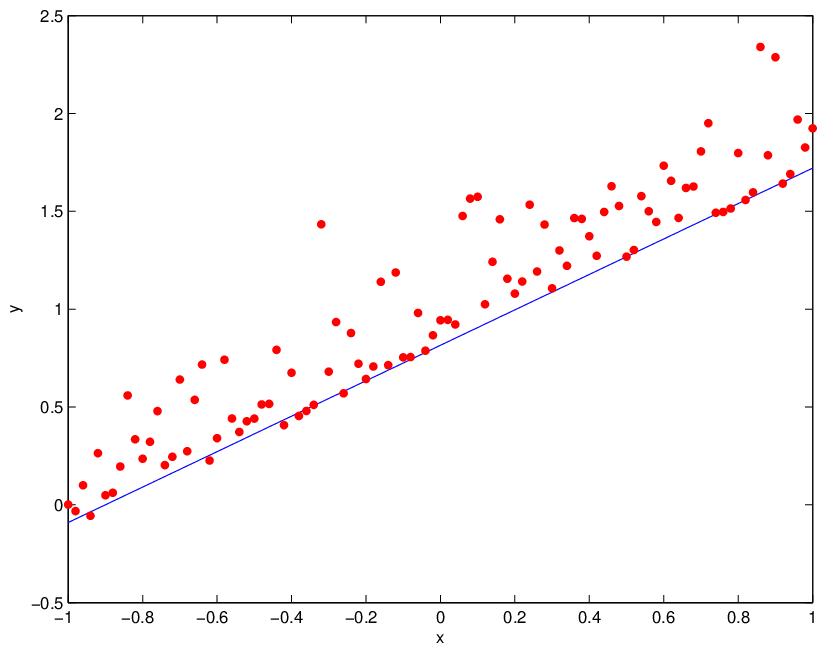
Figure 3 shows an example of using the asymmetric normal with and . The straight line is the noise-less relationship and the dots are the noised samples obtained. Since , the distribution creates less points with negative measurement errors and makes the positive errors larger. From this image, it is clear that a standard normal is not able to fit well the noise, since the region with high concentration of points is close to the line, but it is concentrated on one side of the mean noise.
We performed simulations for each value of , where in each run the values of were sampled uniformly in the interval and the underlying standard deviation was set to . The inputs, which were shared by all simulations, were given by equidistant points between and .


Figure 4(a) shows the resulting likelihood of the fitted model, where the dashed line represents equal likelihood. When , both models exhibit similar likelihoods, as we expected since this case describes the symmetric normal distribution. Furthermore, since the symmetric normal is a particular case of the asymmetric one, its likelihood can not be higher than the likelihood of the asymmetric normal. In fact, the asymmetric normal has higher likelihood in all simulations performed. However, when we set or , both symmetric and asymmetric models have lower likelihood, with the asymmetric one fitting better, as expected. The decrease in likelihood for the asymmetric model can be explained in part by Equation (12c), where we have shown that the model loses likelihood by making more distant from , while the decrease for the symmetric normal is due to incorrect noise modelling.
It is important to highlight that, just like the terms in Equation (11) and in Equation (13) which prevents the error terms in the same equations to have almost no weight, the cost in Equation (12c) can be viewed as an implicit regularization that prevents one side of the partition to have no weight, and this regularization is inherent to the distributions defined in Equations (3) and (7) and is not artificially imposed.
Moreover, there is a similarity between the resulting likelihoods for and . This is expected, since there is a similarity between the two, with favoring positive noises as much as favors negative ones.
Figure 4(b) shows the correct and predicted values of , again with the dashed line representing the identity function, where predicted values are represented by their mean and confidence interval. The mean prediction is clearly close to the true value, and the large variation of fitted weights is due to the small number of samples, since the model is more flexible. However, when comparing the likelihood values for in Figure 4(a), we see that the large spread of predicted values, from to approximately, does not interfere in the likelihood, as the value is similar to the normal that has .
Although it might seem that the results in Figure 4(b) are not the maximum likelihood estimates, since they may be far from the real parameter used to create the noise, we remind the reader that they may differ for a finite number of samples, just like any other estimate. For instance, for samples drawn from the normal distribution, the maximum likelihood estimate for the mean is given by , but this estimate depends on the value of the specific sampled. If we consider the uncertainty on , it can be shown that the estimate is given by (Krishnamoorthy, 2006), which specifies a random variable that only converges to the real value as . Therefore, for finite number of samples, the parameter may differ from and still be a maximum likelihood estimate.
Therefore, we have shown that the asymmetric normal noise model is able to fit as well as the symmetric normal when the noise is indeed symmetric, and outperforms it when there is asymmetry in the noise. This motivates the use of the asymmetric normal distribution as a generalization of the normal distribution, thus being able to adapt to the observed noise asymmetry.
5.2 Hidden Markov Model with Asymmetric Emissions
While the creation of more flexible distributions by introducing the asymmetry is in itself interesting, with the possibility of fitting different data while keeping the interpretability, its use may also provide additional insights of practical relevance. To illustrate the application of the new distributions, we will use a hidden Markov model (HMM) to fit a time-series.
A HMM with states is defined by the initial distribution on the states , the transition matrix between states , and the parameters for each distribution associated with each state . For the normal distribution, is given by and , while for the asymmetric version, is also included. In this application, we will build two HMM, one with only symmetric and one with only asymmetric normal distributions.
To improve the initial estimates for the HMM, we first fit the data using a mixture model with weights and with the same parameters for the emission distributions. Once the expectation maximization algorithm runs for 100 iterations, we set and , such that every sample has the same prior probability over the emission distributions. Additionally, for the asymmetric version, we first fit the samples, both for the mixture and the HMM, using the method described in Section 4.3.
The data used was the Dow Jones Industrial Average index (DJI) from its first quotation, on Jan 29, 1985, to its last quotation of 2014, on Dec 31, 2014, with the prices adjusted for dividends and splits, where we consider that its value follows the lognormal distribution, as usual in the economics field (Aitchison and Brown, 1957). Each sample is composed of the return over investment’s (ROI) logarithm for consecutive days, that is, the sample is given by , where is the quotation in the -th day. If either day of a pair does not have a quotation, what happens if one of them is on a weekend for instance, then that sample is considered missing. Therefore, the HMM has one state for each day between those dates.
The main motivation of using this kind of problem is that the hypothesis of symmetry implied by the normal distribution may not reflect the reality. It is well known that stock markets can have periods of very high or low return, which sometimes characterize bull or bear markets (Edwards et al., 2013). Therefore, we expect to see improvements by introducing an emission distribution that is able to exhibit such asymmetric behavior.
Table 1 shows the final log-likelihood for the samples with different number of possible states . As expected, using the asymmetric distribution provides greater likelihood due to its additional flexibility. Moreover, increasing the number of states also increases the difference in likelihood. Since the number of states in which the HMMs differ the most is given by , the subsequent analysis will consider only this case.
| K | Symmetric | Asymmetric |
|---|---|---|
| 2 | 19310.47 | 19310.91 |
| 3 | 19480.27 | 19481.32 |
| 4 | 19509.24 | 19514.80 |
| 5 | 19519.82 | 19538.44 |
| Source state | Symmetric | Asymmetric |
|---|---|---|
| 1 | 0.1256 | 0.0847 |
| 2 | 1.4972 | 0.4564 |
| 3 | 0.4320 | 0.2108 |
| 4 | 0.1815 | 0.1836 |
| 5 | 1.1986 | 0.3565 |


Figure 5 shows the emission distributions for each HMM, with the mode dashed to highlight the asymmetry. While some asymmetries are more subtle, like in components C4 () and C2 (), others are more noticeable, like C1 () and C5 (). In special, the component C3 has the largest asymmetry of all, with .
Since the shape of the base distribution, in this case the normal distribution, has been preserved in each side, the weight for each case can be used to provide some additional insight into the state. For example, the state associated with the component C3 is considerably certain that the index will rise (), which none of the emissions in the symmetric case indicates.
While the increased likelihood and the presence of asymmetry are expected from using a more general version of the distributions, other interesting and potentially useful results appear when we analyze the distribution over states.


When we evaluate the transition probabilities for each state, shown in Figure 6, it becomes very clear that the transitions for the asymmetric version are usually much less ambiguous. To evaluate this quantitatively, Table 2 shows the entropy of the transitions out of each state, with the maximum entropy being given by bits.
Except for the fourth state, which suffered a minor increase in entropy of and had no noticeable difference in Figure 6, all other transitions reduced the entropy considerably, from to , with clear differences in the transition.


This reduced entropy also occurs in the states themselves, as shown in Figure 7. Figure 7(a) shows the histogram of normalized entropies, which is the entropy divided by the maximum entropy, for both HMMs and considering the state of missing data or not. In both cases, the asymmetric version has considerably more states with lower entropy than the symmetric version. Note also that the asymmetric version appears to suffer less from missing data, while the symmetric version has a spike around that does not occur without considering these states.
To emphasize the difference, Figure 7(b) shows the entropy QQ plot, which is composed of plotting the normalized entropy quantiles of each HMM’s states, with the dashed line representing the identity. From this figure, we note that the symmetric HMM’s states indeed have higher entropy than the ones from the asymmetric, with the first reaching normalized entropy 0.4 before the latter gets , and a quantile with asymmetric distributions almost always has less entropy than its equivalent symmetric, with the only exceptions being the first few quantiles with very low entropy. Additionally, this figure also shows that the curves that considers the missing data is close to the one that does not, also indicating that the asymmetric version has good performance despite this lack of information.
6 Conclusion
In this paper, we have introduced the concept of a constrained mixture and provided two examples of how it can be used with the Laplace and normal distributions to create new asymmetric distributions. The new distributions were shown to generalize their underlying distribution while keeping important properties, such as belonging to the exponential family and having maximum likelihood estimates and conjugate priors with known closed-form expressions. Moreover, the distributions were shown to have an inherent regularization term, that is, a regularization that comes directly from the likelihood and not an imposed cost, that penalizes the asymmetry, such that the distribution avoids unnecessarily deforming the symmetric underlying distribution.
One of the new distributions, the asymmetric normal distribution, was compared to the symmetric version in a regression example with asymmetric noise. This allowed a better understanding of how the asymmetric distributions operate and showed that, since the symmetric versions are particular cases of the asymmetric distributions, the asymmetric ones must have higher likelihood.
The asymmetric and symmetric normal distributions were also compared when used for emissions in a hidden Markov model (HMM) for a stock index. Results show that, as one would expect, the additional flexibility of the asymmetry allowed the distribution to better fit the data, providing increased likelihood and with larger differences as more states were used.
A positive consequence of this flexibility and better fitting was additional certainty in the states and their transitions. We have shown that, when the HMM had 5 states, most probability distributions over the states had a considerable reduction in their entropy even when missing data is considered. Moreover, although one transition distribution, which already exhibited low entropy, had its entropy increased by , all other transitions had reduced entropy, losing from to of their values, and the largest transition entropy is less than of the maximum entropy, compared to for the symmetric version.
Future investigations involve analyzing if it is possible to know the maximum likelihood estimates and conjugate priors and their closed-form expressions for the Laplace and normal distributions when the domain split does not occur at the mode. If so, the effect of using the constrained mixture in other distributions of the exponential family and the use of multiple segments should be investigated. Besides this theoretical research, the use of asymmetry to characterize loss functions in machine learning is of interest, since it can make the system focus more on predicting low or high values.
Acknowledgments
The authors would like to thank CNPq for the financial support.
A Proof of Theorem 2
B Proof of Theorem 5
C Proof of lemma for Theorem 8
Lemma 12
Let and , be given. Let the pdf of the asymmetric Laplace distribution be given by Equation (3). Then the function
where , , and , is convex.
Furthermore, let . If there is some such that , then for all .
Proof Let and . Let . Let be a variable associated with sample , such that
where is the indicator function. Since , we have that and , and .
Let , , , , . Then
which proves that is a convex function.
Moreover, if there is some , then and either
or , so that
for all .
D Proof of Theorem 8
Proof From Equation (11), one can see that can be optimized independently from the value of . Let be defined as in Lemma 12, such that
where is a constant. Therefore, the value that minimizes is the maximum likelihood estimator. The function can be rewritten as
which is associated with the log-likelihood of the weighted scale-free Laplace distribution, whose maximum likelihood estimate is given by the weighted median (Edgeworth, 1888) with samples in and weighting and , respectively.
For , the optimal value is given by:
which solves for the value provided by the theorem.
From Lemma 12, we also know that there is no sample
between two optima and , , of
, or there would be some such that , which contradicts the optimality of
or .
E Proof of Theorem 9
F Proof of lemma for Theorem 10
Lemma 13
Let and , be given. Let the pdf of the asymmetric normal distribution be given by Equation (7). Then the function
where , , and , is strictly convex.
Proof Let be a function and its -th derivative. If and are continuous and for all , then is strictly convex.
For fixed and , is a strictly convex quadratic function of . If is continuously differentiable and its derivative is monotonically increasing for variables and , then is strictly convex.
Let . The limit is given by:
which proves that is continuous. Its derivative is given by:
| (14) |
and we can prove that it is continuous using the same method as before.
Since , the
derivative is monotonically increasing and is
strictly convex.
G Proof of Theorem 10
Proof From Equation (13), one can see that can be optimized independently of the value of . Let be defined as in Lemma 13, such that
where is a constant. Therefore, the value that minimizes is the maximum likelihood estimator. And, since is strictly convex, this value is unique.
From the first order optimality condition, we can solve Equation (14) to find the optimal stated in the theorem. For , the optimal value is given by:
which solves for the value provided by the theorem.
H Proof of Theorem 11
References
- Aitchison and Brown (1957) J. Aitchison and J. A. C. Brown. The Lognormal Distribution with Special Reference to Its Uses in Economics. 1957.
- Banerjee and Shan (2007) A. Banerjee and H. Shan. Latent Dirichlet Conditional Naive-Bayes Models. In International Conference on Data Mining (ICDM), pages 421–426. IEEE, 2007.
- Banerjee et al. (2005) A. Banerjee, S. Merugu, I. S. Dhillon, and J. Ghosh. Clustering with Bregman Divergences. Journal of Machine Learning Research, 6:1705–1749, 2005.
- Barndorff-Nielsen (2014) O. Barndorff-Nielsen. Information and Exponential Families in Statistical Theory. John Wiley & Sons, 2014.
- Baum and Petrie (1966) L. E. Baum and T. Petrie. Statistical Inference for Probabilistic Functions of Finite State Markov Chains. The Annals of Mathematical Statistics, pages 1554–1563, 1966.
- Bianco et al. (2005) A. M. Bianco, M. G. Ben, and V. J. Yohai. Robust Estimation for Linear Regression with Asymmetric Errors. Canadian Journal of Statistics, 33(4):511–528, 2005.
- Bishop (2006) C. M. Bishop. Pattern Recognition and Machine Learning. Springer, 2006.
- Blei et al. (2003) D. M. Blei, A. Y. Ng, and M. I. Jordan. Latent Dirichlet Allocation. Journal of Machine Learning Research, 3:993–1022, 2003.
- Edgeworth (1888) F. Y. Edgeworth. On a New Method of Reducing Observations Relating to Several Quantities. Philosophical Magazines, 1888.
- Edwards et al. (2013) R. D. Edwards, J. Magee, and W. H. C. Bassetti. Technical Analysis of Stock Trends. CRC Press, 2013.
- Geman and Geman (1984) S. Geman and D. Geman. Stochastic Relaxation, Gibbs Distributions, and the Bayesian Restoration of Images. IEEE Transactions on Pattern Analysis and Machine Intelligence, (6):721–741, 1984.
- Johnson et al. (1994) N. L. Johnson, S. Kotz, and N. Balakrishnan. Lognormal Distributions. In Continuous Univariate Distributions, volume 1. Wiley Series in Probability and Mathematical Statistics: Applied Probability and Statistics, 2nd edition, 1994.
- Koller and Friedman (2009) D. Koller and N. Friedman. Probabilistic Graphical Models: Principles and Techniques. MIT press, 2009.
- Krishnamoorthy (2006) K. Krishnamoorthy. Handbook of Statistical Distributions with Applications. CRC Press, 2006.
- Kullback and Leibler (1951) S. Kullback and Richard A. Leibler. On Information and Sufficiency. Annals of Mathematical Statistics, pages 79–86, 1951.
- McLachlan and Basford (1988) G. J. McLachlan and K. E. Basford. Mixture Models: Inference and Applications to Clustering. Applied Statistics, 1988.
- O’Hagan and Leonard (1976) A. O’Hagan and T. Leonard. Bayes Estimation Subject to Uncertainty About Parameter Constraints. Biometrika, 63(1):201–203, 1976.
- Shan and Banerjee (2008) H. Shan and A. Banerjee. Bayesian Co-clustering. In International Conference on Data Mining (ICDM), pages 530–539. IEEE, 2008.