跳到论文正文
W Papers独立论文阅读器 arXiv:1503.06423 论文正文 计算阅读时间 · 0%
引用这篇论文根据当前论文元数据生成,正式投稿前建议核对。


License: arXiv.org perpetual non-exclusive license
arXiv:1503.06423v2 [hep-ph] 31 May 2015

LMU-ASC 11/15 FTUV/15−-0322 IFIC/15−-12 Flavour-changing top decays
in the aligned two-Higgs-doublet model

Gauhar Abbas Affiliation: IFIC, Universitat de València – CSIC, Apt. Correus 22085, E-46071 València, Spain    Alejandro Celis Affiliation: Ludwig-Maximilians-Universität München, Fakultät für PhysikArnold Sommerfeld Center for Theoretical Physics, 80333 München, Germany    Xin-Qiang Li Affiliation: Institute of Particle Physics and Key Laboratory of Quark and Lepton Physics (MOE)Central China Normal University, Wuhan, Hubei 430079, China Affiliation: State Key Laboratory of Theoretical Physics, Institute of Theoretical PhysicsChinese Academy of Sciences, Beijing 100190, China    Jie Lu Affiliation: Department of Physics, Shanghai University, Shanghai 200444, China    Antonio Pich Affiliation: IFIC, Universitat de València – CSIC, Apt. Correus 22085, E-46071 València, Spain

Abstract

We perform a complete one-loop computation of the two-body flavour-changing top decays t→c​ht\rightarrow ch and t→c​Vt\rightarrow cV (V=γ,ZV=\gamma,Z), within the aligned two-Higgs-doublet model. We evaluate the impact of the model parameters on the associated branching ratios, taking into account constraints from flavour data and measurements of the Higgs properties. Assuming that the 125125 GeV Higgs corresponds to the lightest CP-even scalar of the CP-conserving aligned two-Higgs-doublet model, we find that the rates for such flavour-changing top decays lie below the expected sensitivity of the future high-luminosity phase of the LHC. Measurements of the Higgs signal strength in the di-photon channel are found to play an important role in limiting the size of the t→c​ht\rightarrow ch decay rate when the charged scalar of the model is light.

1 Introduction

The discovery of a new boson, with a mass close to 125125 GeV, by the ATLAS [1] and CMS [2] collaborations stands as a remarkable success of the Standard Model (SM) of electroweak interactions. The properties of this boson are so far in agreement with those of the SM Higgs, indicating that the new particle is indeed associated with the mechanism of electroweak symmetry breaking (EWSB). A characteristic feature of the SM is the absence of flavour-changing neutral-current (FCNC) interactions at tree-level. FCNCs are generated through quantum loop corrections in the SM, but they are strongly suppressed by the Glashow–Iliopoulos–Maiani (GIM) mechanism [3].

A widely studied enlargement of the electroweak theory consists in adding a second scalar doublet to the SM field content. The so-called two-Higgs-doublet model (2HDM) represents a minimal extension of the SM scalar sector that easily accommodates electroweak precision data and leads to a very rich phenomenology [4]. In the most general version of the 2HDM unwanted FCNCs appear at tree-level, which represents a major shortcoming of the model. The hypothesis of natural flavour conservation (NFC) is the usual way out to this issue. By limiting the number of scalar doublets coupling to a given type of right-handed fermion to be at most one, the absence of dangerous FCNCs is guaranteed [5, 6]. A more general solution is that of Yukawa alignment [7]. The aligned two-Higgs-doublet model (A2HDM) assumes that the two Yukawa matrices coupled to the same type of right-handed fermion are aligned in flavour space, so that no FCNCs appear at tree level. Explicit models where a Yukawa aligned structure arises due to an underlying symmetry have been discussed in refs. [8, 9, 10, 11, 12]. Interestingly, all different versions of the 2HDM with NFC are recovered as particular limits of the A2HDM. Constraints on the A2HDM from flavour and collider data have been analyzed in refs. [13, 14, 15, 16, 17, 18] and [19, 20, 21, 22, 23, 24, 25, 26], respectively, extracting relevant bounds on the model parameters.

In this work we study the flavour-changing top-quark decays t→c​ht\rightarrow ch and t→c​Vt\rightarrow cV (V=γ,ZV=\gamma,Z), within the framework of the A2HDM. They arise at the loop level and are strongly suppressed in the SM, due to the GIM mechanism. A significant enhancement can be achieved in alternative scenarios of EWSB, making these processes a suitable place to look for new physics beyond the SM. Early considerations of these effects were done in refs. [27, 28, 29, 30, 31, 32]. A concise review of the flavour-changing top-decay phenomenology can be found in ref. [33]. In the A2HDM these decays receive additional charged Higgs contributions at the one-loop level which could lift the decay rates.

Comprehensive analyses of flavour-changing top decays within 2HDMs with NFC have been done in refs. [29, 31, 35, 34]. However, these rare processes have not been investigated yet within the more general setting of the A2HDM. Furthermore, since these studies were performed, considerable experimental progress in our understanding of the EWSB mechanism has been made, translating into tight constraints on possible extensions of the SM scalar sector.

Searches for flavour-changing top decays have been performed recently by the ATLAS [36, 37] and CMS collaborations [38, 40, 39], placing limits on the associated branching ratios. An overview of the current experimental status can be found in ref. [41]. With the large amount of data that will be collected in the future LHC runs, it is expected that these bounds will be improved by at least one order of magnitude [42, 43].

Our paper is organized as follows. In section 2 we introduce the A2HDM. Flavour-changing top decays are discussed in section 3, which presents the results of our calculations. A phenomenological analysis of these processes is given in section 4, and our conclusions are finally summarized in section 5. Explicit analytical results for the relevant decay amplitudes are given in the appendices.

2 Framework

The 2HDM extends the SM scalar sector with an additional complex scalar doublet. In the Higgs basis, where only one doublet acquires vacuum expectation value, the scalar fields are parametrized by [21]

Φ1=[G+12​(v+S1+i​G0)],Φ2=[H+12​(S2+i​S3)],\Phi_{1}=\left[\begin{array}[]{c}G^{+}\\ \frac{1}{\sqrt{2}}\,(v+S_{1}+iG^{0})\end{array}\right]\;,\qquad\qquad\Phi_{2}=\left[\begin{array}[]{c}H^{+}\\ \frac{1}{\sqrt{2}}\,(S_{2}+iS_{3})\end{array}\right]\;, (2.1)

with v=(2GF)−1/2≃246v=(\sqrt{2}G_{F})^{-1/2}\simeq 246 GeV. Here G0,±G^{0,\pm} correspond to the would-be Goldstone bosons, giving mass to the gauge vector bosons, while H±H^{\pm} is a charged Higgs. The scalar spectrum also contains three neutral Higgs bosons φj0​(x)={h⁡(x),H⁡(x),A⁡(x)}\varphi_{j}^{0}(x)=\{h(x),H(x),A(x)\}, given by φj0=ℛj​k​Sk\varphi_{j}^{0}=\mathcal{R}_{jk}S_{k}, where ℛ\mathcal{R} is an orthogonal matrix obtained after diagonalizing the mass terms in the scalar potential [21]. In general none of the neutral Higgs bosons are CP eigenstates.

2.1 Scalar sector

The most general scalar potential allowed by the electroweak gauge symmetry can be written as

V\displaystyle V =\displaystyle= μ1​Φ1†​Φ1+μ2​Φ2†​Φ2+[μ3​Φ1†​Φ2+μ3∗​Φ2†​Φ1]\displaystyle\mu_{1}\;\Phi_{1}^{\dagger}\Phi_{1}\,+\,\mu_{2}\;\Phi_{2}^{\dagger}\Phi_{2}\,+\,\left[\mu_{3}\;\Phi_{1}^{\dagger}\Phi_{2}\,+\,\mu_{3}^{*}\;\Phi_{2}^{\dagger}\Phi_{1}\right] (2.2)
+\displaystyle+ λ1​(Φ1†​Φ1)2+λ2​(Φ2†​Φ2)2+λ3​(Φ1†​Φ1)​(Φ2†​Φ2)+λ4​(Φ1†​Φ2)​(Φ2†​Φ1)\displaystyle\lambda_{1}\,\left(\Phi_{1}^{\dagger}\Phi_{1}\right)^{2}\,+\,\lambda_{2}\,\left(\Phi_{2}^{\dagger}\Phi_{2}\right)^{2}\,+\,\lambda_{3}\,\left(\Phi_{1}^{\dagger}\Phi_{1}\right)\left(\Phi_{2}^{\dagger}\Phi_{2}\right)\,+\,\lambda_{4}\,\left(\Phi_{1}^{\dagger}\Phi_{2}\right)\left(\Phi_{2}^{\dagger}\Phi_{1}\right)
+\displaystyle+ [(λ5Φ1†Φ2+λ6Φ1†Φ1+λ7Φ2†Φ2)(Φ1†Φ2)+h.c.].\displaystyle\biggl[\left(\lambda_{5}\;\Phi_{1}^{\dagger}\Phi_{2}\,+\,\lambda_{6}\;\Phi_{1}^{\dagger}\Phi_{1}\,+\,\lambda_{7}\;\Phi_{2}^{\dagger}\Phi_{2}\right)\left(\Phi_{1}^{\dagger}\Phi_{2}\right)\,+\,\mathrm{h.c.}\,\biggr]\,.

Due to the Hermiticity of the scalar potential, all parameters are real with the exception of μ3,λ5,λ6\mu_{3},\lambda_{5},\lambda_{6} and λ7\lambda_{7}. The minimization conditions impose the relations

μ1=−λ1​v2,μ3=−12​λ6​v2.\mu_{1}\;=\;-\lambda_{1}\,v^{2}\,,\qquad\qquad\qquad\mu_{3}\;=\;-\frac{1}{2}\,\lambda_{6}\,v^{2}\,. (2.3)

The mass of the charged Higgs is given by

MH±2=μ2+12​λ3​v2,M_{H^{\pm}}^{2}\;=\;\mu_{2}+\frac{1}{2}\,\lambda_{3}\,v^{2}\,, (2.4)

while those of the neutral scalars have been obtained in ref. [21] to first order in the CP-violating parameters. In the CP-conserving limit the neutral Higgs bosons are CP eigenstates. The CP-odd field AA corresponds to S3S_{3} and the CP-even states are orthogonal combinations of S1S_{1} and S2S_{2}:

(hH)=[cos⁡α~sin⁡α~−sin⁡α~cos⁡α~]​(S1S2).\left(\begin{array}[]{c}h\\ H\end{array}\right)\;=\;\left[\begin{array}[]{cc}\cos{\tilde{\alpha}}&\sin{\tilde{\alpha}}\\ -\sin{\tilde{\alpha}}&\cos{\tilde{\alpha}}\end{array}\right]\;\left(\begin{array}[]{c}S_{1}\\ S_{2}\end{array}\right)\,. (2.5)

Here Mh⩽MHM_{h}\leqslant M_{H} by convention and the mixing angle α~\tilde{\alpha} is determined by

sin⁡2​α~=−2​λ6​v2MH2−Mh2,cos⁡2​α~=MA2+2​(λ5−λ1)​v2MH2−Mh2.\displaystyle\sin 2\tilde{\alpha}\;=\;\frac{-2\lambda_{6}v^{2}}{M_{H}^{2}-M_{h}^{2}}\,,\qquad\qquad\cos 2\tilde{\alpha}\;=\;\frac{M_{A}^{2}+2(\lambda_{5}-\lambda_{1})v^{2}}{M_{H}^{2}-M_{h}^{2}}\,. (2.6)

In the CP-conserving limit the masses of the neutral Higgs bosons are given by

Mh2=12​(Σ−Δ),MH2=12​(Σ+Δ),MA2=MH±2+v2​(λ42−λ5),M_{h}^{2}\;=\;\frac{1}{2}\,\left(\Sigma-\Delta\right),\quad\quad M_{H}^{2}\;=\;\frac{1}{2}\,\left(\Sigma+\Delta\right),\quad\quad M_{A}^{2}\;=\;M_{H^{\pm}}^{2}\,+\,v^{2}\,\left(\frac{\lambda_{4}}{2}-\lambda_{5}\right), (2.7)

where

Σ\displaystyle\Sigma =\displaystyle\;=\; MH±2+(2​λ1+λ42+λ5)​v2,\displaystyle M_{H^{\pm}}^{2}+\left(2\lambda_{1}+\frac{\lambda_{4}}{2}+\lambda_{5}\right)v^{2}\,, (2.8)
Δ\displaystyle\Delta =\displaystyle\;=\; [MA2+2​(λ5−λ1)​v2]2+4​v4​λ62.\displaystyle\sqrt{\left[M_{A}^{2}+2(\lambda_{5}-\lambda_{1})v^{2}\right]^{2}+4v^{4}\lambda_{6}^{2}}\,. (2.9)

By performing a phase redefinition of the CP-even fields one can restrict the mixing angle to the range 0⩽α~<π0\leqslant\tilde{\alpha}<\pi. Moreover, the Higgs basis of the CP-conserving 2HDM is defined up to a global rephasing of the second Higgs doublet Φ2→−Φ2\Phi_{2}\rightarrow-\Phi_{2} [44, 45]. Without loss of generality, one can then fix the sign of λ6\lambda_{6}; by convention, we choose λ6⩽0\lambda_{6}\leqslant 0 so that 0⩽α~⩽π/20\leqslant\tilde{\alpha}\leqslant\pi/2.

2.2 Yukawa sector

In the A2HDM, the interactions of the physical scalar fields with fermions are described by [7]

ℒY\displaystyle\mathcal{L}_{Y} =\displaystyle= −2v​H+​{u¯​[ςd​V​Md​PR−ςu​Mu†​V​PL]​d+ςl​ν¯​Ml​PR​l}\displaystyle-\frac{\sqrt{2}}{v}\;H^{+}\Bigl\{\bar{u}\left[\varsigma_{d}\,VM_{d}\,P_{R}-\varsigma_{u}\,M_{u}^{\dagger}V\,P_{L}\right]d\,+\,\varsigma_{l}\,\bar{\nu}M_{l}\,P_{R}l\Bigr\} (2.10)
−1v∑φi0,fyfφi0φi0[f¯MfPRf]+h.c.,\displaystyle-\,\frac{1}{v}\;\sum_{\varphi^{0}_{i},f}\,y^{\varphi^{0}_{i}}_{f}\,\varphi^{0}_{i}\;\left[\bar{f}\,M_{f}\,P_{R}f\right]\;+\;\mathrm{h.c.}\,,

where PL,R=(1∓γ5)/2P_{L,R}=(1\mp\gamma_{5})/2 are the chirality projectors, Mf=u,d,lM_{f=u,d,l} represent the diagonal fermion mass matrices, VV is the Cabibbo–Kobayashi–Maskawa (CKM) [46, 47] matrix, and

yd,lφi0=ℛi​1+(ℛi​2+i​ℛi​3)​ςd,l,yuφi0=ℛi​1+(ℛi​2−i​ℛi​3)​ςu∗.y_{d,l}^{\varphi^{0}_{i}}=\mathcal{R}_{i1}+(\mathcal{R}_{i2}+i\,\mathcal{R}_{i3})\,\varsigma_{d,l}\,,\qquad\qquad y_{u}^{\varphi^{0}_{i}}=\mathcal{R}_{i1}+(\mathcal{R}_{i2}-i\,\mathcal{R}_{i3})\,\varsigma_{u}^{*}\,. (2.11)

The parameters ςf\varsigma_{f} (f=u,d,lf=u,d,l) are family-universal complex quantities which introduce new sources of CP violation beyond the CKM matrix. For particular real values of these parameters, indicated in table 1, one recovers all different versions of the 2HDM with NFC.

Table 1: Two-Higgs-doublet models with natural flavour conservation.
Model ςd\varsigma_{d} ςu\varsigma_{u} ςl\varsigma_{l}
Type I cot⁡β\cot{\beta} cot⁡β\cot{\beta} cot⁡β\cot{\beta}
Type II −tan⁡β-\tan{\beta} cot⁡β\cot{\beta} −tan⁡β-\tan{\beta}
Type X (lepton specific) cot⁡β\cot{\beta} cot⁡β\cot{\beta} −tan⁡β-\tan{\beta}
Type Y (flipped) −tan⁡β-\tan{\beta} cot⁡β\cot{\beta} cot⁡β\cot{\beta}

The Yukawa alignment condition is not stable against quantum corrections [7, 13, 48]. However, the flavour symmetries of the A2HDM constrain tightly the possible FCNC effects, keeping them well below present experimental bounds [7, 49, 50, 51, 52]. The only FCNC local structures induced at one-loop take the form [13]

ℒFCNC=\displaystyle\mathcal{L}_{\mbox{\scriptsize{FCNC}}}\;=\; 𝒞4​π2​v3(1+ςu∗ςd)∑jφj0{(ℛj​2+iℛj​3)(ςd−ςu)[d¯LV†MuMu†VMddR]\displaystyle\frac{\mathcal{C}}{4\pi^{2}v^{3}}\,(1+\varsigma_{u}^{*}\varsigma_{d})\sum_{j}\,\varphi_{j}^{0}\,\biggl\{(\mathcal{R}_{j2}+i\mathcal{R}_{j3})(\varsigma_{d}-\varsigma_{u})\Bigl[\bar{d}_{L}\,V^{{\dagger}}M_{u}M_{u}^{{\dagger}}VM_{d}\,d_{R}\Bigr]
−(ℛj​2−iℛj​3)(ςd∗−ςu∗)[u¯LVMdMd†V†MuuR]}+h.c.,\displaystyle-(\mathcal{R}_{j2}-i\mathcal{R}_{j3})(\varsigma_{d}^{*}-\varsigma_{u}^{*})\Bigl[\bar{u}_{L}\,VM_{d}M_{d}^{{\dagger}}V^{{\dagger}}M_{u}u_{R}\Bigr]\biggr\}+\mathrm{h.c.}\,, (2.12)

which vanishes exactly for the 2HDMs with NFC. In general, the size of the induced flavour-changing interactions is controlled by three powers of quark masses and the GIM mechanism.

The renormalization of the coupling constant 𝒞\mathcal{C} is determined, using dimensional regularization, to be [17]

𝒞=𝒞R​(μ)+12​{2​μD−4D−4+γE−ln⁡(4​π)},\mathcal{C}=\mathcal{C}_{R}(\mu)+\frac{1}{2}\left\{\frac{2\mu^{D-4}}{D-4}+\gamma_{E}-\ln(4\pi)\right\}\,, (2.13)

where γE≃0.577\gamma_{E}\simeq 0.577 is the Euler constant and μ\mu is an arbitrary renormalization mass scale. The renormalized coupling satisfies

𝒞R​(μ)=𝒞R​(μ0)−ln⁡(μ/μ0).\mathcal{C}_{R}(\mu)=\mathcal{C}_{R}(\mu_{0})-\ln(\mu/\mu_{0})\,. (2.14)

Assuming Yukawa alignment to be exact at a given energy scale ΛA\Lambda_{A}, so that 𝒞R​(ΛA)=0\mathcal{C}_{R}(\Lambda_{A})=0, implies that 𝒞R​(μ)=ln⁡(ΛA/μ)\mathcal{C}_{R}(\mu)=\ln(\Lambda_{A}/\mu).

3 Flavour-changing top decays

The flavour-changing top decays t→c​ht\rightarrow ch and t→c​Vt\rightarrow cV (V=γ,ZV=\gamma,Z) occur firstly at the one-loop level in the SM. The decay rate for these processes is not only suppressed by the loop factor, but receives in addition a strong CKM and GIM suppression [53, 29, 32, 33]. Here we focus on final states with the charm quark because Br⁡(t→u​X)/Br⁡(t→c​X)≃|Vu​b/Vc​b|2∼7×10−3\mathrm{Br}(t\rightarrow uX)/\mathrm{Br}(t\rightarrow cX)\simeq|V_{ub}/V_{cb}|^{2}\sim 7\times 10^{-3} in the SM, as well as in the A2HDM. Fixing the Higgs mass at Mh≃125M_{h}\simeq 125 GeV, one obtains the SM branching ratios: Br⁡(t→c​h)∼𝒪⁡(10−15)\mathrm{Br}(t\rightarrow ch)\sim\mathcal{O}(10^{-15}), Br⁡(t→c​γ)∼𝒪⁡(10−14)\mathrm{Br}(t\rightarrow c\gamma)\sim\mathcal{O}(10^{-14}) and Br⁡(t→c​Z)∼𝒪⁡(10−14)\mathrm{Br}(t\rightarrow cZ)\sim\mathcal{O}(10^{-14}). Within the A2HDM these decay rates can be enhanced due to additional charged Higgs contributions at the loop level. For t→c​φj0t\rightarrow c\varphi_{j}^{0} decays, the counter-term piece in eq. (2.12) would also contribute.

In the SM, the dominant decay mode of the top quark is the unsuppressed two-body decay t→W+​bt\rightarrow W^{+}b, with Γ⁡(t→W+​b)/mt∼1%\Gamma(t\rightarrow W^{+}b)/m_{t}\sim 1\%. To compute the relevant branching ratios we take

Br⁡(t→c​X)=Γ⁡(t→c​X)Γtot​(t).\mathrm{Br}(t\rightarrow cX)\;=\;\dfrac{\Gamma(t\rightarrow cX)}{\Gamma_{\mbox{\scriptsize{tot}}}(t)}\,. (3.1)

To a very good approximation, Γtot​(t)≃Γ⁡(t→W+​b)\Gamma_{\mbox{\scriptsize{tot}}}(t)\simeq\Gamma(t\rightarrow W^{+}b) holds also in the A2HDM, except when MH±<mt−mbM_{H^{\pm}}<m_{t}-m_{b}; in this case, the additional decay mode t→H+​bt\rightarrow H^{+}b must be taken into account. The partial decay widths for t→W+​bt\rightarrow W^{+}b and t→H+​bt\rightarrow H^{+}b are calculated at leading order:

Γ⁡(t→W+​b)=\displaystyle\Gamma(t\rightarrow W^{+}b)\;= g2​|Vt​b|264​π​mt3​λ1/2​(mt2,mb2,MW2)​[mt2+mb2+(mt2−mb2)2MW2−2​MW2],\displaystyle\;\frac{g^{2}\,|V_{tb}|^{2}}{64\,\pi\,m_{t}^{3}}\;\,\lambda^{1/2}(m_{t}^{2},m_{b}^{2},M_{W}^{2})\,\biggl[m_{t}^{2}+m_{b}^{2}+\frac{(m_{t}^{2}-m_{b}^{2})^{2}}{M_{W}^{2}}-2M_{W}^{2}\biggr]\,, (3.2)
Γ⁡(t→H+​b)=\displaystyle\Gamma(t\rightarrow H^{+}b)\;= |Vt​b|216​π​mt3​v2λ1/2(mt2,mb2,MH±2)[(mt2+mb2−MH±2)(mb2|ςd|2+mt2|ςu|2)\displaystyle\;\frac{|V_{tb}|^{2}}{16\,\pi\,m_{t}^{3}\,v^{2}}\;\,\lambda^{1/2}(m_{t}^{2},m_{b}^{2},M_{H^{\pm}}^{2})\,\biggl[\left(m_{t}^{2}+m_{b}^{2}-M_{H^{\pm}}^{2}\right)\,\left(m_{b}^{2}|\varsigma_{d}|^{2}+m_{t}^{2}|\varsigma_{u}|^{2}\right)\quad
−4mb2mt2Re(ςdςu∗)].\displaystyle\hskip 167.87108pt\mbox{}-4m_{b}^{2}m_{t}^{2}\,\mathrm{Re}\left(\varsigma_{d}\varsigma_{u}^{*}\right)\biggr]\,. (3.3)

Here λ⁡(x,y,z)≡x2+y2+z2−2​(x​y+x​z+y​z)\lambda(x,y,z)\equiv x^{2}+y^{2}+z^{2}-2(xy+xz+yz), and gg is the SU​(2)L\mathrm{SU(2)}_{L} gauge coupling constant.

Due to the smallness of md,sm_{d,s} and the unitarity of the CKM matrix, the t→c​φj0t\rightarrow c\varphi_{j}^{0} and t→c​Vt\rightarrow cV decay amplitudes turn out to be very sensitive to the bottom quark mass [33]. The most adequate choice for the internal quark masses is the running MS¯\overline{\rm MS} quark mass evaluated at a typical scale 𝒪⁡(mt)\mathcal{O}(m_{t}) [33]; we follow this prescription. The external quark masses are taken as the on-shell pole masses.

In section 3.1 we describe the calculation of the t→c​φj0t\rightarrow c\varphi_{j}^{0} decay amplitudes. The decays t→c​Vt\rightarrow cV (V=γ,ZV=\gamma,Z) are discussed in section 3.2. Explicit analytical results for these processes within the A2HDM are collected in the appendices. All our results are presented in the Feynman gauge, corresponding to ξ=1\xi=1 in the RξR_{\xi} gauge. We have however checked the gauge independence of our results by additionally performing all calculations in the unitary gauge. We have also checked analytically that our results reproduce the corresponding SM predictions [27, 29, 32].

3.1 𝐭→𝐜​𝝋𝐣𝟎\mathbf{\boldsymbol{t\rightarrow c\,\varphi_{j}^{0}}} decays

The total amplitude for t⁡(pt)→c⁡(pc)​φj0​(pφ)t(p_{t})\rightarrow c(p_{c})\,\varphi_{j}^{0}(p_{\varphi}) decays can be written as Atot=A+ActA_{\mbox{\scriptsize{tot}}}=A+A_{\mbox{\scriptsize{ct}}}. Here AA collects all the contributions arising from one-loop diagrams and can be parametrized as [27, 29]

A=∑n=118An=∑n=118∑q=d,s,bVc​q​Vt​q∗​u¯​(pc)​[α(n)​PR+β(n)​PL]​u​(pt).A\;=\;\sum_{n=1}^{18}\,A_{n}\;=\;\sum_{n=1}^{18}\sum_{q=d,s,b}\,V_{cq}V_{tq}^{*}\;\,\bar{u}(p_{c})\Bigl[\alpha^{(n)}\,P_{R}+\beta^{(n)}\,P_{L}\Bigr]u(p_{t})\,. (3.4)

Diagrams contributing to this process in the Feynman gauge are shown in figures 1 and 2. The total loop amplitude is ultraviolet divergent, except in the particular cases of 2HDMs with NFC where a finite result is obtained. As expected, the divergence gets reabsorbed into the renormalization of the counter-term coupling 𝒞\mathcal{C} in eq. (2.12). The tree-level contribution of the counter-term Lagrangian takes the form

Act=∑q=d,s,bVc​q​Vt​q∗​u¯​(pc)​[αct​PR+βct​PL]​u​(pt),A_{\mbox{\scriptsize{ct}}}\;=\;\sum_{q=d,s,b}V_{cq}V_{tq}^{*}\;\,\bar{u}(p_{c})\Bigl[\alpha_{\mbox{\scriptsize{ct}}}\,P_{R}+\beta_{\mbox{\scriptsize{ct}}}\,P_{L}\Bigr]u(p_{t})\,, (3.5)

with

αct=\displaystyle\alpha_{\mbox{\scriptsize{ct}}}\;=\; −𝒞​i​g3​mt32​π2​MW3​(1+ςu∗​ςd)​(ςd−ςu)∗​(ℛj​2−i​ℛj​3)​mq2,\displaystyle-\mathcal{C}\,\frac{ig^{3}m_{t}}{32\pi^{2}M_{W}^{3}}\,(1+\varsigma_{u}^{*}\varsigma_{d})(\varsigma_{d}-\varsigma_{u})^{*}(\mathcal{R}_{j2}-i\mathcal{R}_{j3})\,m_{q}^{2}\,,
βct=\displaystyle\beta_{\mbox{\scriptsize{ct}}}\;=\; −𝒞​i​g3​mc32​π2​MW3​(1+ςd∗​ςu)​(ςd−ςu)​(ℛj​2+i​ℛj​3)​mq2.\displaystyle-\mathcal{C}\,\frac{ig^{3}m_{c}}{32\pi^{2}M_{W}^{3}}\,(1+\varsigma_{d}^{*}\varsigma_{u})(\varsigma_{d}-\varsigma_{u})(\mathcal{R}_{j2}+i\mathcal{R}_{j3})\,m_{q}^{2}\,. (3.6)
Figure 1: Penguin diagrams contributing to t→c​φj0t\rightarrow c\varphi_{j}^{0} in the Feynman gauge.
Figure 2: Self-energy diagrams contributing to t→c​φj0t\rightarrow c\varphi_{j}^{0} in the Feynman gauge.

The partial decay width can be written as

Γ⁡(t→c​φj0)=λ1/2​(mt2,mc2,Mφj02)32​π​mt3​[(|α|2+|β|2)​(mc2+mt2−Mφj02)+2​mc​mt​(α∗​β+β∗​α)].\displaystyle\Gamma(t\rightarrow c\,\varphi_{j}^{0})\;=\;\dfrac{\lambda^{1/2}(m_{t}^{2},m_{c}^{2},M_{\varphi_{j}^{0}}^{2})}{32\,\pi\,m_{t}^{3}}\,\left[(|\alpha|^{2}+|\beta|^{2})(m_{c}^{2}+m_{t}^{2}-M_{\varphi_{j}^{0}}^{2})+2m_{c}m_{t}\,(\alpha^{*}\beta+\beta^{*}\alpha)\right]. (3.7)

Here

α=∑q=d,s,bVc​q​Vt​q∗​(∑n=118α(n)+αct),β=∑q=d,s,bVc​q​Vt​q∗​(∑n=118β(n)+βct).\displaystyle\alpha\;=\;\sum_{q=d,s,b}V_{cq}V_{tq}^{*}\;\left(\sum_{n=1}^{18}\alpha^{(n)}+\alpha_{\mbox{\scriptsize{ct}}}\right)\,,\qquad\quad\beta\;=\;\sum_{q=d,s,b}V_{cq}V_{tq}^{*}\;\left(\sum_{n=1}^{18}\beta^{(n)}+\beta_{\mbox{\scriptsize{ct}}}\right)\,. (3.8)

The contributions to the amplitude from each diagram, encoded in the coefficients α(n)\alpha^{(n)} and β(n)\beta^{(n)}, are collected in appendix B.

3.2 𝐭→𝐜𝐕⁡(𝐕=𝜸,𝐙)\mathbf{\boldsymbol{t\rightarrow cV~(V=\gamma,Z)}} decays

The decays t⁡(pt)→c⁡(pc)​V​(pV)t(p_{t})\rightarrow c(p_{c})\,V(p_{V}) can only proceed at the loop level (there are no tree-level counter-terms in this case). The decay amplitude can be parametrized as [29]

A=∑n=114Anμ​ϵμ∗​(pV)=\displaystyle A\;=\;\sum_{n=1}^{14}A^{\mu}_{n}\,\epsilon_{\mu}^{*}(p_{V})\;=\; ∑n=114∑q=d,s,bVc​qVt​q∗u¯(pc){[a1(n)pVμ+a2(n)ptμ+a3(n)γμ]PL\displaystyle\sum_{n=1}^{14}\sum_{q=d,s,b}\,V_{cq}V_{tq}^{*}\;\bar{u}(p_{c})\biggl\{\left[a_{1}^{(n)}\,p_{V}^{\mu}+a_{2}^{(n)}\,p_{t}^{\mu}+a_{3}^{(n)}\,\gamma^{\mu}\right]\,P_{L}
+[b1(n)pVμ+b2(n)ptμ+b3(n)γμ]PR}u(pt)ϵμ∗(pV),\displaystyle+\left[b_{1}^{(n)}\,p_{V}^{\mu}+b_{2}^{(n)}\,p_{t}^{\mu}+b_{3}^{(n)}\,\gamma^{\mu}\right]\,P_{R}\biggr\}u(p_{t})\;\epsilon_{\mu}^{*}(p_{V})\,, (3.9)

where ϵμ\epsilon_{\mu} is the polarization vector of the gauge boson VV. The one-loop diagrams contributing to this process in the Feynman gauge are shown in figures 3 and 4. The total amplitude is of course ultraviolet finite.

Figure 3: Penguin diagrams contributing to t→c​Vt\rightarrow cV (V=γ,Z)(V=\gamma,Z) in the Feynman gauge.
Figure 4: Self-energy diagrams contributing to t→c​Vt\rightarrow cV (V=γ,Z)(V=\gamma,Z) in the Feynman gauge.

The partial decay widths for t→c​Vt\rightarrow c\,V (V=γ,ZV=\gamma,Z) decays are given, in the limit mc=0m_{c}=0, by

Γ⁡(t→c​γ)=\displaystyle\Gamma(t\rightarrow c\gamma)\;=\; −mt32​π{mt2[|a2|2+|b2|2]−2[|a3|2+|b3|2]+mt2Re(a1∗a2)+mt2Re(b1∗b2)\displaystyle-\dfrac{m_{t}}{32\,\pi}\,\biggl\{m_{t}^{2}\,\bigl[|a_{2}|^{2}+|b_{2}|^{2}\bigr]-2\,\bigl[|a_{3}|^{2}+|b_{3}|^{2}\bigr]+m_{t}^{2}\,\mathrm{Re}(a_{1}^{*}a_{2})+m_{t}^{2}\,\mathrm{Re}(b_{1}^{*}b_{2})
+2mtRe[a3∗(b1+b2)]+2mtRe[b3∗(a1+a2)]},\displaystyle\qquad\qquad+2m_{t}\,\mathrm{Re}\bigl[a_{3}^{*}(b_{1}+b_{2})\bigr]+2m_{t}\,\mathrm{Re}\bigl[b_{3}^{*}(a_{1}+a_{2})\bigr]\biggr\}\,, (3.10)

and

Γ⁡(t→c​Z)=\displaystyle\Gamma(t\rightarrow cZ)\;=\; (mt2−MZ2)2128​π​mt3​MZ2{(mt2−MZ2)2[|a2|2+|b2|2]+4(mt2+2MZ2)[|a3|2+|b3|2]\displaystyle\dfrac{(m_{t}^{2}-M_{Z}^{2})^{2}}{128\,\pi\,m_{t}^{3}\,M_{Z}^{2}}\,\biggl\{(m_{t}^{2}-M_{Z}^{2})^{2}\,\bigl[|a_{2}|^{2}+|b_{2}|^{2}\bigr]+4\,(m_{t}^{2}+2M_{Z}^{2})\,\bigl[|a_{3}|^{2}+|b_{3}|^{2}\bigr]
+4mt(mt2−MZ2)[Re(a2b3∗)+Re(a3b2∗)]}.\displaystyle\qquad\qquad\qquad\quad\;+4m_{t}\,(m_{t}^{2}-M_{Z}^{2})\,\bigl[\mathrm{Re}(a_{2}b_{3}^{*})+\mathrm{Re}(a_{3}b_{2}^{*})\bigr]\biggr\}\,. (3.11)

Here we have defined

ai=∑q=d,s,bVc​q​Vt​q∗​(∑n=114ai(n)),bi=∑q=d,s,bVc​q​Vt​q∗​(∑n=114bi(n)),\displaystyle a_{i}\;=\;\sum_{q=d,s,b}V_{cq}V_{tq}^{*}\,\left(\sum_{n=1}^{14}a_{i}^{(n)}\right)\,,\qquad\quad b_{i}\;=\;\sum_{q=d,s,b}V_{cq}V_{tq}^{*}\,\left(\sum_{n=1}^{14}b_{i}^{(n)}\right)\,, (3.12)

with i=1,2,3i=1,2,3. For the numerical analysis we always keep finite charm mass effects into account. The contributions to the amplitude from each diagram, encoded in the coefficients ai(n)a_{i}^{(n)} and bi(n)b_{i}^{(n)}, are collected in appendix C.

4 Discussion

Relevant inputs for the evaluation of the flavour-changing top decay rates are listed in table 2. We assume that the combined measurement of the top-quark mass by the Tevatron and the LHC corresponds to the pole mass, but we increase its systematic error by 11 GeV to account for the intrinsic ambiguity in the top-quark mass definition. The bottom- and charm-quark masses quoted in the table are MS¯\overline{\rm MS} running masses at the quark-mass scale, i.e., m¯q​(m¯q)\overline{m}_{q}(\overline{m}_{q}), while the light-quark ones are MS¯\overline{\rm MS} running masses renormalized at a scale of 22 GeV. To fix the needed entries of the CKM matrix we use inputs with a minimal sensitivity to new physics contributions. Our SM predictions for the processes considered are presented in table 3.

Table 2: Relevant inputs for the evaluation of the decay rates.
Input Value Comment Input Value Comment
GFG_{F} 1.1663787​(6)×10−51.1663787(6)\times 10^{-5} GeV-2 Ref. [54] MhM_{h} 125.14​(24)125.14(24) GeV Refs. [60, 61]
MWM_{W} 80.385​(15)80.385(15) GeV Ref. [54] mtm_{t} 173.34​(1.76)173.34(1.76) GeV Refs. [62, 63, 64]
MZM_{Z} 91.1876​(21)91.1876(21) GeV Ref. [54] mbm_{b} 4.18​(3)4.18(3) GeV Ref. [54]
γCKM\gamma_{\text{\scriptsize{CKM}}} (73.2−7.0+6.3)∘(73.2_{-7.0}^{+6.3})^{\circ} Ref. [55] mcm_{c} 1.275​(25)1.275(25) GeV Ref. [54]
|Vu​s||V_{us}| 0.2247​(7)0.2247(7) Ref. [56] msm_{s} 93.8​(2.4)×10−393.8(2.4)\times 10^{-3} GeV Ref. [56]
|Vu​b||V_{ub}| 3.42​(15)×10−33.42(15)\times 10^{-3} Ref. [56] mdm_{d} 4.68​(16)×10−34.68(16)\times 10^{-3} GeV Ref. [56]
|Vc​b||V_{cb}| 42.21​(78)×10−342.21(78)\times 10^{-3} Refs. [57, 58, 59] αs​(MZ)\alpha_{s}(M_{Z}) 0.1185​(6)0.1185(6) Ref. [54]
Table 3: SM predictions for flavour-changing top decays.
   Observable       SM prediction   
   Br⁡(t→c​γ)\mathrm{Br}(t\rightarrow c\gamma)       (4.31±0.24)×10−14(4.31\pm 0.24)\times 10^{-14}   
   Br⁡(t→c​Z)\mathrm{Br}(t\rightarrow cZ)       (1.03±0.06)×10−14(1.03\pm 0.06)\times 10^{-14}   
   Br⁡(t→c​h)\mathrm{Br}(t\rightarrow ch)       (3.00±0.17)×10−15(3.00\pm 0.17)\times 10^{-15}   

The ATLAS and CMS collaborations have searched for flavour-changing decays of the top quark. The ATLAS collaboration sets the bound Br⁡(t→q​Z)<0.73%\mathrm{Br}(t\rightarrow qZ)<0.73\% at the 95%95\% confidence level (CL), with 2.12.1 fb-1 of data at s=7\sqrt{s}=7 TeV [36], where the qq in the final state denotes a sum over q=u,cq=u,c. The CMS collaboration has set a better limit, Br⁡(t→q​Z)<0.05%\mathrm{Br}(t\rightarrow qZ)<0.05\%, with 24.724.7 fb-1 of data at s=7& 8\sqrt{s}=7\,\&\,8 TeV [38]. The strongest current bound on t→c​γt\rightarrow c\gamma decay has been obtained by the CMS collaboration, Br⁡(t→c​γ)<0.182%\mathrm{Br}(t\rightarrow c\gamma)<0.182\%, using 19.119.1 fb-1 of data at s=8\sqrt{s}=8 TeV [39].11 1 The CMS limit quoted here on Br⁡(t→c​γ)\mathrm{Br}(t\rightarrow c\gamma) is actually derived from a search for the anomalous single top quark production in association with a photon in proton-proton collisions, following an effective Lagrangian approach with the assumption of vanishing contributions from both t​q​gtqg and t​u​γtu\gamma interactions [39]. The ATLAS collaboration sets the limit Br⁡(t→q​h)<0.79%\mathrm{Br}(t\rightarrow qh)<0.79\%, with 2525 fb-1 of data at s=7& 8\sqrt{s}=7\,\&\,8 TeV [37]. A slightly stronger limit, Br⁡(t→q​h)<0.56%\mathrm{Br}(t\rightarrow qh)<0.56\%, has been obtained by the CMS collaboration, using 19.5 fb-1 of data at s=8\sqrt{s}=8 TeV [40]. Future prospects for these processes at the high luminosity LHC have been discussed in refs. [42, 43]. One expects to improve the limits to the 10−510^{-5} level for Br⁡(t→c​V)\mathrm{Br}(t\rightarrow cV) (V=γ,ZV=\gamma,Z), while for Br⁡(t→c​h)\mathrm{Br}(t\rightarrow ch) it would be possible to reach the 10−4−10−510^{-4}-10^{-5} level.

For the phenomenological discussion we shall focus on the CP-conserving A2HDM, which contains 1212 free real parameters: μ2\mu_{2}, λk\lambda_{k} (k=1,…,7)(k=1,\ldots,7), the three alignment constants ςf\varsigma_{f} (f=u,d,l)(f=u,d,l) and the counter-term coupling 𝒞R​(μ)\mathcal{C}_{R}(\mu). Physical amplitudes are independent of the renormalization scale μ\mu, due to eq. (2.14); in the following, we choose μ=MW\mu=M_{W}. Some of the parameters of the scalar potential can be traded by the physical scalar masses and the mixing angle α~\tilde{\alpha}. The following relations

λ1\displaystyle\lambda_{1} =12​v2​[Mh2​cos2⁡α~+MH2​sin2⁡α~],λ4=1v2​[Mh2​sin2⁡α~+MH2​cos2⁡α~+MA2−2​MH±2],\displaystyle=\frac{1}{2v^{2}}\left[M_{h}^{2}\,\cos^{2}\tilde{\alpha}+M_{H}^{2}\,\sin^{2}\tilde{\alpha}\right]\,,\quad\quad\lambda_{4}=\frac{1}{v^{2}}\left[M_{h}^{2}\,\sin^{2}\tilde{\alpha}+M_{H}^{2}\,\cos^{2}\tilde{\alpha}+M_{A}^{2}-2M_{H^{\pm}}^{2}\right]\,,
λ5\displaystyle\lambda_{5} =12​v2​[Mh2​sin2⁡α~+MH2​cos2⁡α~−MA2],λ6=−1v2​(MH2−Mh2)​cos⁡α~​sin⁡α~,\displaystyle=\frac{1}{2v^{2}}\left[M_{h}^{2}\,\sin^{2}\tilde{\alpha}+M_{H}^{2}\,\cos^{2}\tilde{\alpha}-M_{A}^{2}\right]\,,\quad\quad\lambda_{6}=-\frac{1}{v^{2}}(M_{H}^{2}-M_{h}^{2})\cos\tilde{\alpha}\,\sin\tilde{\alpha}\,, (4.1)

together with eq. (2.4), allow us to work with a set of parameters more closely related to physical quantities:

Scalar sector: Mh,MH,MA,MH±,cosα~,λ2,λ3,λ7,\displaystyle\text{Scalar sector: \ }\hskip 7.11317ptM_{h},M_{H},M_{A},M_{H^{\pm}},\cos\tilde{\alpha},\lambda_{2},\lambda_{3},\lambda_{7}\,,
Yukawa sector: ςu,ςd,ςl,𝒞R(MW).\displaystyle\text{Yukawa sector: \ }\varsigma_{u},\varsigma_{d},\varsigma_{l},\mathcal{C}_{R}(M_{W})\,. (4.2)

Not all the parameters are relevant for the processes we are concerned about. The decays t→c​φj0t\rightarrow c\,\varphi_{j}^{0} are only sensitive to {Mφj0M_{\varphi_{j}^{0}}, MH±M_{H^{\pm}}, cos⁡α~\cos\tilde{\alpha}, λ3\lambda_{3}, λ7\lambda_{7}, ςu\varsigma_{u}, ςd\varsigma_{d}, 𝒞R​(MW)\mathcal{C}_{R}(M_{W})}. The transition amplitude does not depend on the other neutral scalar masses Mφi0M_{\varphi_{i}^{0}} (i≠ji\neq j), as can be seen explicitly from eq. (B.2). There is also no dependence on the coupling λ2\lambda_{2}; the associated term in the scalar potential (Φ2†​Φ2)2(\Phi_{2}^{{\dagger}}\Phi_{2})^{2} does not generate the needed cubic vertices H+​H−​φj0H^{+}H^{-}\varphi_{j}^{0} because Φ2\Phi_{2} has no vacuum expectation value (see eq. (2.1)). The decays t→c​Vt\rightarrow cV (V=γ,ZV=\gamma,Z), on the other hand, depend only on MH±M_{H^{\pm}} and the alignment parameters ςu,d\varsigma_{u,d}. All the relevant cubic vertices are fixed in this case by the gauge symmetry and do not depend on free parameters of the scalar potential.

We assume in the following that the 125125 GeV Higgs boson corresponds to the lightest CP-even state hh; i.e., we fix Mh≃125M_{h}\simeq 125 GeV. The LHC data imply that it couples to the massive gauge vector bosons with a SM-like strength so that cos⁡α~≃1\cos\tilde{\alpha}\simeq 1. We are interested in how large the enhancements of the flavour-changing top decay rates can be, compared with the SM predictions, focusing on the 125125 GeV Higgs boson in the case of t→c​φj0t\rightarrow c\,\varphi_{j}^{0} transitions. To address this question, we analyze the parameter space of the A2HDM, subject to the following assumptions and constraints:

  • •

    The LHC and Tevatron Higgs data imply that cos⁡α~>0.9\cos\tilde{\alpha}>0.9 (68%68\% CL) and |yfh|∼1|y^{h}_{f}|\sim 1 (f=u,d,lf=u,d,l) [21, 25]. We work in the limit cos⁡α~=1\cos\tilde{\alpha}=1 so that no constraints on the alignment parameters are obtained from the 125125 GeV Higgs data [21, 25].

  • •

    We take into account constraints in the ςu−ςd\varsigma_{u}-\varsigma_{d} plane derived from the measurement of Br⁡(B¯→Xs​γ)\mathrm{Br}(\bar{B}\rightarrow X_{s}\gamma) [13, 14].

  • •

    We restrict the alignment parameter |ςu|≤2|\varsigma_{u}|\leq 2, in order to satisfy the constraints from Z→b¯​bZ\rightarrow\bar{b}b decay and Bs,d0−B¯s,d0B_{s,d}^{0}-\bar{B}_{s,d}^{0} mixings [13]. The parameters ςd,l\varsigma_{d,l} are much less constrained phenomenologically; we take |ςd,ℓ|≤50|\varsigma_{d,\ell}|\leq 50 as in ref. [14].

  • •

    The four LEP collaborations, ALEPH, DELPHI, L3 and OPAL, have searched for pair-produced charged Higgs bosons in the framework of 2HDMs, excluding MH±≲80M_{H^{\pm}}\lesssim 80 GeV (95%95\% CL) under the assumption that H±H^{\pm} decays dominantly into fermions [65].

  • •

    Searches for a light charged Higgs via the decay t→H+​bt\rightarrow H^{+}b performed by the ATLAS [66, 67] and CMS [68, 69] collaborations, together with the limits on a charged Higgs from the Tevatron [70], are taken into account. These direct searches give an upper bound on the Yukawa combination |ςu​ςd||\varsigma_{u}\varsigma_{d}|, which, although being weaker than the one from Br⁡(B¯→Xs​γ)\mathrm{Br}(\bar{B}\rightarrow X_{s}\gamma), basically exclude one of the two possible strips allowed by the latter [25].

  • •

    We consider the perturbativity bound on the quartic scalar couplings |λ3,7|≤4​π|\lambda_{3,7}|\leq 4\pi [21]. Additionally, the loop-induced decay h→γ​γh\rightarrow\gamma\gamma is sensitive to λ3\lambda_{3} and λ7\lambda_{7} through the charged Higgs contribution to this process [21, 25]. We take into account the latest measurements of the Higgs signal strengths in the h→γ​γh\rightarrow\gamma\gamma channel by ATLAS [71] and CMS [61].

In the limit cos⁡α~=1\cos\tilde{\alpha}=1, the decay rate for t→c​ht\rightarrow ch does not depend on 𝒞R​(MW)\mathcal{C}_{R}(M_{W}) and λ7\lambda_{7}. Explicit expressions for all the relevant cubic Higgs couplings are provided in appendix B. In particular, for cos⁡α~=1\cos\tilde{\alpha}=1 we have λH+​H−h=λ3\lambda_{H^{+}H^{-}}^{h}=\lambda_{3}. The measured Higgs signal strengths by ATLAS and CMS in the di-photon channel are then only sensitive to λ3\lambda_{3} and MH±M_{H^{\pm}}. Since in this case the Higgs production cross-section is the same as in the SM, one can write the Higgs signal strength in the di-photon channel as [21, 25]:

μγ​γh=σ⁡(p​p→h)×Br⁡(h→2​γ)σ​(p​p→h)SM×Br​(h→2​γ)SM≃(1−0.15​CH±h)2,\mu_{\gamma\gamma}^{h}\;=\;\frac{\sigma(pp\rightarrow h)\times\mathrm{Br}(h\rightarrow 2\gamma)}{\sigma(pp\rightarrow h)_{\mbox{\scriptsize{SM}}}\times\mathrm{Br}(h\rightarrow 2\gamma)_{\mbox{\scriptsize{SM}}}}\;\simeq\;\left(1-0.15\,C_{H^{\pm}}^{h}\right)^{2}\,, (4.3)

where CH±hC_{H^{\pm}}^{h} encodes the charged Higgs contribution to h→2​γh\rightarrow 2\gamma and is given by

CH±h=v22​MH±2​λH+​H−h​𝒜​(xH±).C_{H^{\pm}}^{h}\;=\;\frac{v^{2}}{2M_{H^{\pm}}^{2}}\,\lambda_{H^{+}H^{-}}^{h}\,\mathcal{A}(x_{H^{\pm}})\,. (4.4)

Here

𝒜⁡(x)=−x−x24​f​(x),f⁡(x)=−4​arcsin2⁡(1/x),\mathcal{A}(x)\;=\;-x-\frac{x^{2}}{4}\,f(x)\,,\qquad\qquad f(x)\;=\;-4\arcsin^{2}(1/\sqrt{x})\,, (4.5)

with xH±=4​MH±2/Mh2x_{H^{\pm}}=4M_{H^{\pm}}^{2}/M_{h}^{2}. We require that the Higgs signal strength in eq. (4.3) lies within the 2​σ2\sigma range of the experimental measurements. The latest results by ATLAS [71]: μγ​γh=1.17−0.26+0.28\mu_{\gamma\gamma}^{h}=1.17^{+0.28}_{-0.26}, and by CMS [61]: μγ​γh=1.12±0.24\mu_{\gamma\gamma}^{h}=1.12\pm 0.24, are consistent with the SM.

Performing a scan over {ςu\{\varsigma_{u}, ςd\varsigma_{d}, ςl\varsigma_{l}, λ3}\lambda_{3}\}, subject to the restrictions specified above, while fixing the charged Higgs mass to benchmark values, we obtain the upper bounds on Br⁡(t→c​V)\mathrm{Br}(t\rightarrow cV) (V=γ,ZV=\gamma,Z) and Br⁡(t→c​h)\mathrm{Br}(t\rightarrow ch) shown in table 4. In the window 90​GeV<MH±<150​GeV90~\text{GeV}<M_{H^{\pm}}<150~\text{GeV} the alignment parameter ςd\varsigma_{d} is constrained to be small by the direct charged Higgs searches at the LHC via top decays, |ςd|≲10|\varsigma_{d}|\lesssim 10, implying a very strong suppression on the decay rates. For MH±<90​GeVM_{H^{\pm}}<90~\text{GeV} a weaker bound on |ςd||\varsigma_{d}| is obtained by a combination of LHC and Tevatron limits, |ςd|≲25|\varsigma_{d}|\lesssim 25. For MH±>150M_{H^{\pm}}>150 GeV the largest decay rates for these processes are obtained for |ςu|<1|\varsigma_{u}|<1 and |ςd|≃50|\varsigma_{d}|\simeq 50. The upper bounds obtained for Br⁡(t→c​V)\mathrm{Br}(t\rightarrow cV) put these processes well beyond the reach of the high luminosity LHC, within the A2HDM [43]. Similar conclusions were obtained in refs. [35, 34] within the framework of 2HDMs with NFC.

The decay rate for t→c​ht\rightarrow ch can receive on the other hand much larger enhancements, due to the intermediate charged Higgs contribution involving the cubic Higgs coupling λH+​H−h\lambda_{H^{+}H^{-}}^{h}. The maximum values for Br⁡(t→c​h)\mathrm{Br}(t\rightarrow ch) are obtained when the cubic scalar coupling λH+​H−h\lambda_{H^{+}H^{-}}^{h} saturates either the h→2​γh\rightarrow 2\gamma limits or the perturbativity bound. Diagram 3 in figure 1 dominates the corresponding decay amplitude in this case. The contribution from this diagram to the decay amplitude is proportional to ςu​ςd​λH+​H−h\varsigma_{u}\varsigma_{d}\lambda_{H^{+}H^{-}}^{h} and ςd2​λH+​H−h\varsigma_{d}^{2}\lambda_{H^{+}H^{-}}^{h}, see table 5. While the product ςu​ςd\varsigma_{u}\varsigma_{d} is constrained to be small in magnitude by Br⁡(B¯→Xs​γ)\mathrm{Br}(\bar{B}\rightarrow X_{s}\gamma), the term proportional to ςd2\varsigma_{d}^{2} becomes greatly enhanced for large |ςd||\varsigma_{d}| values. Such large values of |ςd||\varsigma_{d}| can be obtained outside the window 90​GeV<MH±<16090~\text{GeV}<M_{H^{\pm}}<160 GeV since the limits from direct charged Higgs searches via top decays at the LHC are avoided.

Analyses of t→c​ht\rightarrow ch decay within the type II 2HDM, prior to the Higgs discovery, have found that a light charged Higgs can enhance considerably the associated decay rate in this model, for large values of tan⁡β\tan\beta and the cubic Higgs coupling λH+​H−h\lambda_{H^{+}H^{-}}^{h}, and even reach the level of expected sensitivity at the high luminosity LHC: Br⁡(t→c​h)∼10−5\mathrm{Br}(t\rightarrow ch)\sim 10^{-5} [35, 34]. Such behavior is compatible with our findings, given that in the limit ςd=−ςu−1=−tan⁡β\varsigma_{d}=-\varsigma_{u}^{-1}=-\tan\beta we recover the Yukawa couplings of the type II 2HDM. However, we find that current measurements of the 125125 GeV Higgs properties play an important role when evaluating possible enhancements of Br⁡(t→c​h)\mathrm{Br}(t\rightarrow ch). In particular, measurements of the Higgs signal strengths in the di-photon channel restrict the allowed size of the cubic Higgs coupling λH+​H−h\lambda_{H^{+}H^{-}}^{h} for a light charged Higgs. This in turn implies that the allowed enhancements of Br⁡(t→c​h)\mathrm{Br}(t\rightarrow ch) cannot be as large as previously speculated. Taking into account the measurements of the 125125 GeV Higgs properties, searches for a light charged Higgs via top decays, and the flavour constraints specified earlier, we find that the decay rate for t→c​ht\rightarrow ch lies beyond the reach of the high luminosity LHC in 2HDMs without tree-level FCNCs. Under the constraints considered the largest decay rate is obtained for MH±M_{H^{\pm}} being slightly below 9090 GeV, Br⁡(t→c​h)≲2×10⁻⁷\mathrm{Br}(t\rightarrow ch)\lesssim 2\times 10^{-7}.

It is necessary to discuss the robustness of the previous statement. If small deviations from the limit cos⁡α~=1\cos\tilde{\alpha}=1 are considered, the LHC Higgs data gives rise to strong bounds on the magnitude of the alignment parameters. Since |yfh|=|cos⁡α~+ςf​sin⁡α~||y_{f}^{h}|=|\cos\tilde{\alpha}+\varsigma_{f}\sin\tilde{\alpha}| (f=u,d,lf=u,d,l) is constrained to be close to one, one obtains |ςf|≲𝒪⁡(1)|\varsigma_{f}|\lesssim\mathcal{O}(1) when cos⁡α~<1\cos\tilde{\alpha}<1 [21, 25]. This implies in particular that |ςd||\varsigma_{d}| should be small and large enhancements of Br⁡(t→c​h)\mathrm{Br}(t\rightarrow ch) are not possible. Allowing for CP violation would not led to any significant enhancement either, given the strong constraints on CP-violating couplings derived from electric dipole moment experiments [16].

Table 4: Upper bounds for Br⁡(t→c​V)\mathrm{Br}(t\rightarrow cV) (V=γ,ZV=\gamma,Z) and Br⁡(t→c​h)\mathrm{Br}(t\rightarrow ch) in the CP-conserving A2HDM.
   MH±M_{H^{\pm}} [GeV]       Br⁡(t→c​γ)\mathrm{Br}(t\rightarrow c\gamma)       Br⁡(t→c​Z)\mathrm{Br}(t\rightarrow cZ)       Br⁡(t→c​h)\mathrm{Br}(t\rightarrow ch)   
   100       ≲2×10⁻¹²\lesssim 2\times 10^{-12}       ≲2×10⁻¹³\lesssim 2\times 10^{-13}       ≲6×10⁻⁹\lesssim 6\times 10^{-9}   
   200       ≲10−10\lesssim 10^{-10}       ≲3×10⁻¹¹\lesssim 3\times 10^{-11}       ≲3×10⁻⁸\lesssim 3\times 10^{-8}   
   300       ≲10−11\lesssim 10^{-11}       ≲5×10⁻¹²\lesssim 5\times 10^{-12}       ≲2×10⁻⁸\lesssim 2\times 10^{-8}   
   400       ≲2×10⁻¹²\lesssim 2\times 10^{-12}       ≲2×10⁻¹²\lesssim 2\times 10^{-12}       ≲5×10⁻⁹\lesssim 5\times 10^{-9}   
   500       ≲10−12\lesssim 10^{-12}       ≲10−12\lesssim 10^{-12}       ≲2×10⁻⁹\lesssim 2\times 10^{-9}   
   Exp. limit       <1.8×10⁻³<1.8\times 10^{-3} [39]       <5×10⁻⁴<5\times 10^{-4} [38]       <5.6×10⁻³<5.6\times 10^{-3} [40]   

We turn now to discuss the role of the direct counter-term contribution to t→c​ht\rightarrow ch decay, which is not present in 2HDMs with NFC. In the limit cos⁡α~=1\cos\tilde{\alpha}=1 this contribution vanishes because of the orthogonality of ℛ\mathcal{R}. The LHC data imply that cos⁡α~\cos\tilde{\alpha} is very close to one so that the counter-term contribution to the flavour-changing t→c​ht\rightarrow ch decay will be suppressed by a small factor sin⁡α~\sin\tilde{\alpha} at the amplitude level. Furthermore, the characteristic flavour structure of the A2HDM counter-term (2.12) implies a strong suppression of its effects, due to the explicit powers of quark masses and the unitarity of the quark mixing matrix [7]. Neglecting the loop contribution (at μ=MW\mu=M_{W}),

Br​(t→c​h)tree≈\displaystyle\mathrm{Br}(t\to ch)_{\mathrm{tree}}\,\approx\;\, α2​π2​|Vc​b|2​mb42​sin4⁡θW​MW4​(1−Mh2/mt2)2(1−MW2/mt2)2​(1+2​MW2/mt2)​sin2⁡α~​|Ed|2\displaystyle\frac{\alpha^{2}\,\pi^{2}\,|V_{cb}|^{2}\,m_{b}^{4}}{2\,\sin^{4}{\theta_{W}}\,M_{W}^{4}}\;\frac{(1-M_{h}^{2}/m_{t}^{2})^{2}}{(1-M_{W}^{2}/m_{t}^{2})^{2}\,(1+2M_{W}^{2}/m_{t}^{2})}\,\sin^{2}{\tilde{\alpha}}\,|E_{d}|^{2}
≈\displaystyle\;\approx\;\, 2×10⁻¹¹​sin2⁡α~​|Ed|2,\displaystyle 2\times 10^{-11}\,\sin^{2}{\tilde{\alpha}}\,|E_{d}|^{2}\,, (4.6)

where

Ed=14​π2​𝒞R​(MW)​(1+ςu​ςd)​(ςd−ςu).E_{d}\;=\;\frac{1}{4\pi^{2}}\,\mathcal{C}_{R}(M_{W})\,\left(1+\varsigma_{u}\varsigma_{d}\right)\left(\varsigma_{d}-\varsigma_{u}\right)\,. (4.7)

The size of EdE_{d} is constrained experimentally by the measured amount of mixing between the neutral Bs0B_{s}^{0} meson and its antiparticle, which receives also contributions from the Lagrangian (2.12), mediated by the three neutral scalars φi0={h,H,A}\varphi^{0}_{i}=\{h,H,A\}. One finds that this process allows for |Ed|∼𝒪⁡(1)|E_{d}|\sim\mathcal{O}(1), even when the masses of the neutral scalars are of 𝒪⁡(100​GeV)\mathcal{O}(100~\text{GeV}) [49], but this is far too small to generate any observable signal in t→c​ht\to ch.22 2 Assuming Yukawa alignment to hold at the high-energy scale ΛA\Lambda_{A}, we have 𝒞R​(MW)=ln⁡(ΛA/MW)\mathcal{C}_{R}(M_{W})=\ln(\Lambda_{A}/M_{W}). Therefore, 𝒞R​(MW)/(4​π2)≲1\mathcal{C}_{R}(M_{W})/(4\pi^{2})\lesssim 1 for ΛA≲1019\Lambda_{A}\lesssim 10^{19} GeV.

It is important to analyze also the impact of the perturbativity bound on the results obtained. A different upper limit on the relevant cubic coupling |λH+​H−h||\lambda_{H^{+}H^{-}}^{h}| has been considered in ref. [21]. The charged Higgs gives the following finite correction to the h​H+​H−hH^{+}H^{-} vertex, at the one-loop level:

(λH+​H−h)eff=λH+​H−h​[1+v2​(λH+​H−h)216​π2​MH±2​𝒵​(Mh2MH±2)]≡λH+​H−h​(1+Δ),\displaystyle(\lambda_{H^{+}H^{-}}^{h})_{\mbox{\scriptsize{eff}}}\;=\;\lambda_{H^{+}H^{-}}^{h}\,\left[1+\frac{v^{2}(\lambda_{H^{+}H^{-}}^{h})^{2}}{16\pi^{2}M_{H^{\pm}}^{2}}\,\mathcal{Z}\left(\frac{M_{h}^{2}}{M_{H^{\pm}}^{2}}\right)\right]\;\equiv\;\lambda_{H^{+}H^{-}}^{h}\;\left(1+\Delta\right)\,, (4.8)

where

𝒵⁡(X)=∫01d​y​∫01−yd​z​[(y+z)2+X⁡(1−y−z−y​z)]−1.\mathcal{Z}(X)\;=\;\int_{0}^{1}dy\;\int_{0}^{1-y}dz\;\left[(y+z)^{2}+X\,(1-y-z-yz)\right]^{-1}\,. (4.9)

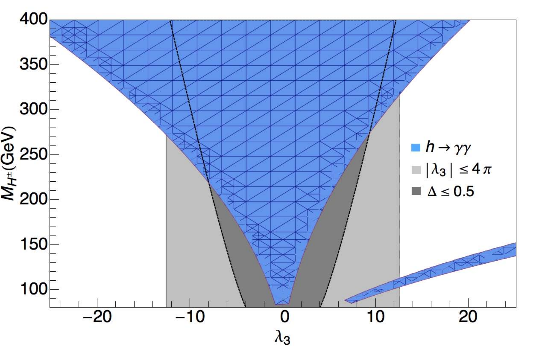
Large values of |λH+​H−h||\lambda_{H^{+}H^{-}}^{h}| could make this loop correction comparable to the leading-order result, which would cast doubts on the perturbative expansion. We therefore allow this correction to be at most 50%50\% (Δ⩽0.5\Delta\leqslant 0.5). In figure 5 we show the region allowed at 2​σ2\sigma by the measurement of the Higgs signal strengths in the di-photon channel, together with the bounds extracted with the perturbativity limits |λ3|⩽4​π|\lambda_{3}|\leqslant 4\pi and Δ⩽0.5\Delta\leqslant 0.5.

Refer to caption
Figure 5: Allowed region by measurements of the Higgs signal strengths in the di-photon channel (blue-meshed) together with the perturbativity limits |λ3|⩽4​π|\lambda_{3}|\leqslant 4\pi (light gray) or Δ⩽0.5\Delta\leqslant 0.5 (dark gray). See text for details.

The constraints from h→γ​γh\rightarrow\gamma\gamma give rise to a large allowed region, centered around λ3=0\lambda_{3}=0, whose width increases for higher values of MH±M_{H^{\pm}}. In this area the h→γ​γh\rightarrow\gamma\gamma decay amplitude is dominated by the WW-boson and top-quark loop contributions, as in the SM; the charged Higgs contribution remains subdominant. For light charged Higgs masses a small disjoint allowed region appears with λ3≳6\lambda_{3}\gtrsim 6. In this small area the charged Higgs contribution dominates over the WW-boson and top-quark loops and flips the sign of the amplitude, (1−0.15​CH±h)∼−1(1-0.15\,C_{H^{\pm}}^{h})\sim-1, giving a SM-like Higgs signal strength (see eq. (4.3)). In principle there is no reason to expect such an accidental tuning of the charged Higgs contribution to occur. This separate small region is therefore not to be seen as very realistic. It is possible to argue that such region brings problems to the perturbative expansion. The perturbativity limit Δ⩽0.5\Delta\leqslant 0.5, being more stringent for light charged Higgs masses, excludes this small region. For a light charged Higgs the maximum values of Br⁡(t→c​h)\mathrm{Br}(t\rightarrow ch) are obtained precisely in this separate region, where the value for |λH+​H−h||\lambda_{H^{+}H^{-}}^{h}| reaches its maximum allowed value. The limits on Br⁡(t→c​h)\mathrm{Br}(t\rightarrow ch) would therefore be even stronger for a light charged Higgs if the perturbativity limit Δ⩽0.5\Delta\leqslant 0.5 is taken into account. Once this perturbativity limit is considered, we get the limit Br⁡(t→c​h)≲6×10⁻⁸\mathrm{Br}(t\rightarrow ch)\lesssim 6\times 10^{-8}.

Recent works have studied the possibility to look for flavour-changing top-quark anomalous interactions via production processes. In ref. [72] a fully gauge-invariant effective-field-theory approach was adopted for parametrizing the top-quark FCNC interactions, while in ref. [73] it was assumed that the Higgs boson posses tree-level flavour-changing couplings with the top quark. It was pointed out in these works that these top-quark flavour-changing effects can often be probed with better sensitivities in production processes than via the top-quark decays. Whether this is also the case within the A2HDM with a light charged scalar deserves a detailed analysis but lies beyond the scope of the present work.

5 Conclusions

We have performed a complete one-loop calculation of flavour-changing top decays (t→c​γt\rightarrow c\gamma, t→c​Zt\rightarrow cZ, t→c​φj0t\rightarrow c\varphi_{j}^{0}), within the A2HDM. Here φj0={h,H,A}\varphi_{j}^{0}=\{h,H,A\} represents any of the neutral scalar mass eigenstates. Our results agree with the available SM results in the literature when the corresponding limit is taken [27, 29]. We have also checked the gauge independence of our results by carrying out the calculation in the Feynman and unitary gauges. Explicit analytical expressions in the Feynman gauge are provided in appendices B and C. The results are presented in the limit mc=0m_{c}=0, in order to avoid lengthy expressions; however, in our numerical analyses we have always used the exact expressions.

The SM predictions for these transitions are given in table 3. They are orders of magnitude too small to be accessible even at the high-luminosity phase of the LHC. We have investigated whether significant enhancements of the branching ratios could be possible within the A2HDM. Assuming that the 125125 GeV Higgs-like boson corresponds to the lightest CP-even state hh of the CP-conserving A2HDM, we have discussed the impact of the relevant model parameters on the decay rates. We have taken into account the constraints from flavour experiments as well as the measurements of the Higgs-boson properties at the LHC. Upper bounds obtained for these rare top decays within the A2HDM are listed in table 4 for benchmark values of the charged Higgs mass.

While sizeable enhancements are indeed possible, compared with the SM predictions, we find that the decay rates for t→c​Vt\rightarrow cV (V=γ,ZV=\gamma,Z) remain well below the expected sensitivity levels at the high luminosity LHC, across all of the parameter space considered. As long as the charged Higgs is relatively light, the decay rate for t→c​ht\rightarrow ch receives much larger enhancements for large values of ςd\varsigma_{d} and the cubic Higgs coupling λH+​H−h\lambda_{H^{+}H^{-}}^{h}. The LHC measurements of the Higgs signal strengths in the di-photon channel are found to play a very important role in estimating the maximum allowed values for Br⁡(t→c​h)\mathrm{Br}(t\rightarrow ch). The charged Higgs also contributes at the loop level to the decay h→γ​γh\rightarrow\gamma\gamma and, for a light charged Higgs, a large cubic coupling λH+​H−h\lambda_{H^{+}H^{-}}^{h} would led to large deviations of the Higgs signal strengths in the di-photon channel. We find that Br⁡(t→c​h)\mathrm{Br}(t\rightarrow ch) lies also beyond the reach of the high luminosity LHC, once the constraints from the Higgs data are taken into account.

Acknowledgments

This work has been supported in part by the Spanish Government and the European Commission [grants FPA2011-23778 and CSD2007-00042 (Consolider Project CPAN)], and the Generalitat Valenciana [PrometeoII/2013/007]. The work of A.C. is supported by the Alexander von Humboldt Foundation. The work of X.L. is supported by the National Natural Science Foundation of China (NSFC) under contract Nos. 11005032 and 11435003. X.L. is also supported in part by the Scientific Research Foundation for the Returned Overseas Chinese Scholars, State Education Ministry, by the Open Project Program of State Key Laboratory of Theoretical Physics, Institute of Theoretical Physics, Chinese Academy of Sciences, China (No.Y4KF081CJ1), and by the self-determined research funds of CCNU from the colleges’ basic research and operation of MOE (CCNU15A02037).

Appendix A Loop functions

Dimensional regularization is used in our calculations. The scalar loop functions appearing are given by [74]

A0​(M1)\displaystyle A_{0}(M_{1}) =∫dD​k~​1k2−M12,\displaystyle\;=\;\int d^{D}\tilde{k}\;\dfrac{1}{k^{2}-M_{1}^{2}}\,,
B0​(l,M1,M2)\displaystyle B_{0}(l,M_{1},M_{2}) =∫dD​k~​1(k2−M12)​[(k+l)2−M22],\displaystyle\;=\;\int d^{D}\tilde{k}\;\dfrac{1}{(k^{2}-M_{1}^{2})[(k+l)^{2}-M_{2}^{2}]}\,,
C0​(l,s,M1,M2,M3)\displaystyle C_{0}(l,s,M_{1},M_{2},M_{3}) =∫dD​k~​1(k2−M12)​[(k+l)2−M22]​[(k+l+s)2−M32].\displaystyle\;=\;\int d^{D}\tilde{k}\;\dfrac{1}{(k^{2}-M_{1}^{2})[(k+l)^{2}-M_{2}^{2}][(k+l+s)^{2}-M_{3}^{2}]}\,. (A.1)

Here

dD​k~=μ3​ϵ/2​dD​k(2​π)D,d^{D}\tilde{k}\;=\;\mu^{3\epsilon/2}\,\dfrac{d^{D}k}{(2\pi)^{D}}\,, (A.2)

is the integration measure with ϵ=4−D\epsilon=4-D, and g​μϵ/2g\mu^{\epsilon/2} is the SU​(2)L\mathrm{SU(2)}_{L} gauge coupling constant in DD dimensions. Vector and tensor integrals are reduced to the scalar loop integrals via the Passarino–Veltman method [75]. Following the notation of refs. [27, 76], we have

B1\displaystyle B_{1} =12​l2​[A0​(M1)−A0​(M2)−s1​B0],\displaystyle\;=\;\frac{1}{2l^{2}}\bigl[A_{0}(M_{1})-A_{0}(M_{2})-s_{1}B_{0}\bigr]\,,
C~0\displaystyle\widetilde{C}_{0} =B0​(s,M2,M3)+M12​C0,\displaystyle\;=\;B_{0}(s,M_{2},M_{3})+M_{1}^{2}C_{0}\,, (A.3)

where s1=l2+M12−M22s_{1}=l^{2}+M_{1}^{2}-M_{2}^{2}. The other relevant loop functions are given by

(C11C12)\displaystyle\left(\begin{array}[]{c}C_{11}\\ C_{12}\end{array}\right)\; =Y⁡[B0​(l+s,M1,M3)−B0​(s,M2,M3)−s1​C0B0​(l,M1,M2)−B0​(l+s,M1,M3)−s2​C0],\displaystyle=\;Y\left[\begin{array}[]{c}B_{0}(l+s,M_{1},M_{3})-B_{0}(s,M_{2},M_{3})-s_{1}C_{0}\\[5.69046pt] B_{0}(l,M_{1},M_{2})-B_{0}(l+s,M_{1},M_{3})-s_{2}C_{0}\end{array}\right]\,,
(C21C23)\displaystyle\left(\begin{array}[]{c}C_{21}\\ C_{23}\end{array}\right)\; =Y⁡[B1​(l+s,M1,M3)+B0​(s,M2,M3)−s1​C11−2​C24B1​(l,M1,M2)−B1​(l+s,M1,M3)−s2​C11],\displaystyle=\;Y\left[\begin{array}[]{c}B_{1}(l+s,M_{1},M_{3})+B_{0}(s,M_{2},M_{3})-s_{1}C_{11}-2C_{24}\\[5.69046pt] B_{1}(l,M_{1},M_{2})-B_{1}(l+s,M_{1},M_{3})-s_{2}C_{11}\end{array}\right]\,,

and

C22=\displaystyle C_{22}\;=\; 12​[l2​s2−(l⋅s)2]{−l⋅s[B1(l+s,M1,M3)−B1(s,M2,M3)−s1C12]\displaystyle\dfrac{1}{2\bigl[l^{2}s^{2}-(l\cdot s)^{2}\bigr]}\;\biggl\{-l\cdot s\Bigl[B_{1}(l+s,M_{1},M_{3})-B_{1}(s,M_{2},M_{3})-s_{1}C_{12}\Bigr]
+l2[−B1(l+s,M1,M3)−s2C12−2C24]},\displaystyle+l^{2}\Bigl[-B_{1}(l+s,M_{1},M_{3})-s_{2}C_{12}-2C_{24}\Bigr]\biggr\}\,,
C24=\displaystyle C_{24}\;=\; 12​(D−2)​[B0​(s,M2,M3)+2​M12​C0+s1​C11+s2​C12].\displaystyle\frac{1}{2(D-2)}\Bigl[B_{0}(s,M_{2},M_{3})+2M_{1}^{2}C_{0}+s_{1}C_{11}+s_{2}C_{12}\Bigr]\,. (A.12)

Here we have defined s2=s2+2​l⋅s+M22−M32s_{2}=s^{2}+2l\cdot s+M_{2}^{2}-M_{3}^{2} and

Y=12​[l2​s2−(l⋅s)2]​[s2−l⋅s−l⋅sl2].Y=\;\dfrac{1}{2\bigl[l^{2}s^{2}-(l\cdot s)^{2}\bigr]}\,\left[\begin{array}[]{cc}s^{2}&-l\cdot s\\[5.69046pt] -l\cdot s&l^{2}\end{array}\right]\,. (A.13)

Appendix B Decay amplitude for 𝐭→𝐜​𝝋𝐣𝟎\mathbf{\boldsymbol{t\rightarrow c\,\varphi_{j}^{0}}}

We parametrize the one-loop contribution to the t→c​φj0t\rightarrow c\,\varphi_{j}^{0} decay amplitude as indicated in eq. (3.4). In table 5 we give the analytical expressions for the coefficients α(n)\alpha^{(n)} and β(n)\beta^{(n)}, obtained from the 1818 Feynman diagrams in figures 1 and 2. For simplicity, we only give the results in the limit mc=0m_{c}=0, although we have used the exact expressions, including finite charm masses, in our numerical results. In this limit, all coefficients β(n)=0\beta^{(n)}=0 (n=1,…,18n=1,\ldots,18), while α(n)=0\alpha^{(n)}=0 for n=15,16,17,18n=15,16,17,18.

We have defined the combination

γdφj0≡ℛj​1+ℛj​2​Re​(ςd)−ℛj​3​Im​(ςd).\gamma_{d}^{\varphi_{j}^{0}}\;\equiv\;\mathcal{R}_{j1}+\mathcal{R}_{j2}\;\mathrm{Re}(\varsigma_{d})-\mathcal{R}_{j3}\;\mathrm{Im}(\varsigma_{d})\,. (B.1)

The matrix ℛ\mathcal{R} determines the neutral Higgs boson states in terms of the neutral components of the scalar doublets in the Higgs basis (see sec. 2). The parameters yu,dφj0y_{u,d}^{\varphi_{j}^{0}} appearing in table 5 have been defined in eq. (2.11). The relevant cubic couplings in this case read [17]

λW+​W−φj0=\displaystyle\lambda_{W^{+}W^{-}}^{\varphi_{j}^{0}}\;=\;\; λG+​W−φj0=ℛj​1,\displaystyle\lambda_{G^{+}W^{-}}^{\varphi_{j}^{0}}\;=\;\mathcal{R}_{j1}\,,
λH+​W−φj0=\displaystyle\lambda_{H^{+}W^{-}}^{\varphi_{j}^{0}}\;=\;\; ℛj​2−i​ℛj​3,\displaystyle\mathcal{R}_{j2}-i\,\mathcal{R}_{j3}\,,
λH+​H−φj0=\displaystyle\lambda_{H^{+}H^{-}}^{\varphi_{j}^{0}}\;=\;\; λ3​ℛj​1+λ7R​ℛj​2−λ7I​ℛj​3,\displaystyle\lambda_{3}\,\mathcal{R}_{j1}+\lambda_{7}^{R}\,\mathcal{R}_{j2}-\lambda_{7}^{I}\,\mathcal{R}_{j3}\,,
λG+​G−φj0=\displaystyle\lambda_{G^{+}G^{-}}^{\varphi_{j}^{0}}\;=\;\; 2​λ1​ℛj​1+λ6R​ℛj​2−λ6I​ℛj​3=Mφj02v2​ℛj​1,\displaystyle 2\lambda_{1}\,\mathcal{R}_{j1}+\lambda_{6}^{R}\,\mathcal{R}_{j2}-\lambda_{6}^{I}\,\mathcal{R}_{j3}\;=\;\frac{M_{\varphi_{j}^{0}}^{2}}{v^{2}}\;\mathcal{R}_{j1}\,,
λH+​G−φj0=\displaystyle\lambda_{H^{+}G^{-}}^{\varphi_{j}^{0}}\;=\;\; λ6​ℛj​1+12​(λ4+2​λ5)​ℛj​2−i2​(λ4−2​λ5)​ℛj​3=Mφj02−MH±2v2​(ℛj​2−i​ℛj​3).\displaystyle\lambda_{6}\,\mathcal{R}_{j1}+\frac{1}{2}\,(\lambda_{4}+2\lambda_{5})\,\mathcal{R}_{j2}-\frac{i}{2}\,(\lambda_{4}-2\lambda_{5})\,\mathcal{R}_{j3}\;=\;\frac{M_{\varphi_{j}^{0}}^{2}-M_{H^{\pm}}^{2}}{v^{2}}\;(\mathcal{R}_{j2}-i\,\mathcal{R}_{j3})\,. (B.2)

Here λkR,I\lambda_{k}^{R,I} denote the real and imaginary parts of λk\lambda_{k} respectively.

Table 5: Amplitude for t→c​φj0t\rightarrow c\,\varphi_{j}^{0} in the limit mc=0m_{c}=0.
nn α(n)\hskip 18.49988pt\hskip 18.49988pt\alpha^{(n)} argument
1 −​g3​mq2​mt4​MW3ςd{ςu∗(ydφj0)∗C~0+mq2(ςu−ςd)∗ydφj0C0-\dfrac{\rule{0.0pt}{11.38092pt}g^{3}m_{q}^{2}m_{t}}{4M_{W}^{3}}\varsigma_{d}\Bigl\{\varsigma_{u}^{*}\,(y_{d}^{\varphi_{j}^{0}})^{*}\,\tilde{C}_{0}+m_{q}^{2}(\varsigma_{u}-\varsigma_{d})^{*}\,y_{d}^{\varphi_{j}^{0}}\,C_{0} (pφj0,−pt,mq,mq,MH±)(p_{\varphi_{j}^{0}},-p_{t},m_{q},m_{q},M_{H^{\pm}})
−[2mq2ςd∗γdφj0−Mφj02ςu∗(ydφj0)∗](C11−C12)}-\bigl[2m_{q}^{2}\varsigma_{d}^{*}\gamma_{d}^{\varphi_{j}^{0}}-M_{\varphi_{j}^{0}}^{2}\varsigma_{u}^{*}\,(y_{d}^{\varphi_{j}^{0}})^{*}\bigr](C_{11}-C_{12})\Bigr\}
2 ​g3​mq2​mt4​MW3​{[2​mq2​γdφj0−Mφj02​(ydφj0)∗]​(C11−C12)−(ydφj0)∗​C~0}\dfrac{\rule{0.0pt}{11.38092pt}g^{3}m_{q}^{2}m_{t}}{4M_{W}^{3}}\Bigl\{\bigl[2m_{q}^{2}\gamma_{d}^{\varphi_{j}^{0}}-M_{\varphi_{j}^{0}}^{2}(y_{d}^{\varphi_{j}^{0}})^{*}\bigr](C_{11}-C_{12})-(y_{d}^{\varphi_{j}^{0}})^{*}\tilde{C}_{0}\Bigr\} (pφj0,−pt,mq,mq,MW)(p_{\varphi_{j}^{0}},-p_{t},m_{q},m_{q},M_{W})
3 −​g​mq2​mtMW​λH+​H−φj0​ςd​{ςu∗​C0+ςd∗​(C11−C12)}-\dfrac{\rule{0.0pt}{11.38092pt}gm_{q}^{2}m_{t}}{M_{W}}\lambda_{H^{+}H^{-}}^{\varphi_{j}^{0}}\varsigma_{d}\Bigl\{\varsigma_{u}^{*}C_{0}+\varsigma_{d}^{*}(C_{11}-C_{12})\Bigr\} (pφj0,−pt,MH±,MH±,mq)(p_{\varphi_{j}^{0}},-p_{t},M_{H^{\pm}},M_{H^{\pm}},m_{q})
4 −​g​mq2​mtMW​λH+​G−φj0​{ςu∗​C0+ςd∗​(C11−C12)}-\dfrac{\rule{0.0pt}{11.38092pt}gm_{q}^{2}m_{t}}{M_{W}}\lambda_{H^{+}G^{-}}^{\varphi_{j}^{0}}\Bigl\{\varsigma_{u}^{*}C_{0}+\varsigma_{d}^{*}(C_{11}-C_{12})\Bigr\} (pφj0,−pt,MW,MH±,mq)(p_{\varphi_{j}^{0}},-p_{t},M_{W},M_{H^{\pm}},m_{q})
5 −​g​mq2​mtMW​(λH+​G−φj0)∗​ςd​(C0+C11−C12)-\dfrac{\rule{0.0pt}{11.38092pt}gm_{q}^{2}m_{t}}{M_{W}}(\lambda_{H^{+}G^{-}}^{\varphi_{j}^{0}})^{*}\varsigma_{d}\Bigl(C_{0}+C_{11}-C_{12}\Bigr) (pφj0,−pt,MH±,MW,mq)(p_{\varphi_{j}^{0}},-p_{t},M_{H^{\pm}},M_{W},m_{q})
6 −​g​mq2​mtMW​λG+​G−φj0​(C0+C11−C12)-\dfrac{\rule{0.0pt}{11.38092pt}gm_{q}^{2}m_{t}}{M_{W}}\lambda_{G^{+}G^{-}}^{\varphi_{j}^{0}}\Bigl(C_{0}+C_{11}-C_{12}\Bigr) (pφj0,−pt,MW,MW,mq)(p_{\varphi_{j}^{0}},-p_{t},M_{W},M_{W},m_{q})
7 (D−2)​​g3​mq2​mt4​MW​{(ydφj0)∗​C0+2​γdφj0​(C11−C12)}(D-2)\dfrac{\rule{0.0pt}{11.38092pt}g^{3}m_{q}^{2}m_{t}}{4M_{W}}\Bigl\{(y_{d}^{\varphi_{j}^{0}})^{*}C_{0}+2\gamma_{d}^{\varphi_{j}^{0}}(C_{11}-C_{12})\Bigr\} (pφj0,−pt,mq,mq,MW)(p_{\varphi_{j}^{0}},-p_{t},m_{q},m_{q},M_{W})
8 −​g3​mt4​MWλH+​W−φj0{ςu∗C~0+2[mq2ςd∗+ςu∗(Mφj02−mt2)]C0-\dfrac{\rule{0.0pt}{11.38092pt}g^{3}m_{t}}{4M_{W}}\lambda_{H^{+}W^{-}}^{\varphi_{j}^{0}}\Bigl\{\varsigma_{u}^{*}\tilde{C}_{0}+2\bigl[m_{q}^{2}\varsigma_{d}^{*}+\varsigma_{u}^{*}(M_{\varphi_{j}^{0}}^{2}-m_{t}^{2})\bigr]C_{0} (pφj0,−pt,MW,MH±,mq)(p_{\varphi_{j}^{0}},-p_{t},M_{W},M_{H^{\pm}},m_{q})
+[mq2ςd∗+(3Mφj02−mt2)ςu∗]C11−[mq2ςd∗+ςu∗(Mφj02+mt2)]C12}+\bigl[m_{q}^{2}\varsigma_{d}^{*}+(3M_{\varphi_{j}^{0}}^{2}-m_{t}^{2})\varsigma_{u}^{*}\bigr]C_{11}-\bigl[m_{q}^{2}\varsigma_{d}^{*}+\varsigma_{u}^{*}(M_{\varphi_{j}^{0}}^{2}+m_{t}^{2})\bigr]C_{12}\Bigr\}
9 ​g3​mt4​MWλG+​W−φj0{−C~0−2(mq2+Mφj02−mt2)C0\dfrac{\rule{0.0pt}{11.38092pt}g^{3}m_{t}}{4M_{W}}\lambda_{G^{+}W^{-}}^{\varphi_{j}^{0}}\Bigl\{-\tilde{C}_{0}-2(m_{q}^{2}+M_{\varphi_{j}^{0}}^{2}-m_{t}^{2})C_{0} (pφj0,−pt,MW,MW,mq)(p_{\varphi_{j}^{0}},-p_{t},M_{W},M_{W},m_{q})
+(mt2−mq2−3Mφj02)C11+(mq2+Mφj02+mt2)C12}+(m_{t}^{2}-m_{q}^{2}-3M_{\varphi_{j}^{0}}^{2})C_{11}+(m_{q}^{2}+M_{\varphi_{j}^{0}}^{2}+m_{t}^{2})C_{12}\Bigr\}
10 ​g3​mq2​mt4​MW​ςd​(λH+​W−φj0)∗​{C0−C11+C12}\dfrac{\rule{0.0pt}{11.38092pt}g^{3}m_{q}^{2}m_{t}}{4M_{W}}\varsigma_{d}(\lambda_{H^{+}W^{-}}^{\varphi_{j}^{0}})^{*}\Bigl\{C_{0}-C_{11}+C_{12}\Bigr\} (pφj0,−pt,MH±,MW,mq)(p_{\varphi_{j}^{0}},-p_{t},M_{H^{\pm}},M_{W},m_{q})
11 ​g3​mq2​mt4​MW​(λG+​W−φj0)∗​{C0−C11+C12}\dfrac{\rule{0.0pt}{11.38092pt}g^{3}m_{q}^{2}m_{t}}{4M_{W}}(\lambda_{G^{+}W^{-}}^{\varphi_{j}^{0}})^{*}\Bigl\{C_{0}-C_{11}+C_{12}\Bigr\} (pφj0,−pt,MW,MW,mq)(p_{\varphi_{j}^{0}},-p_{t},M_{W},M_{W},m_{q})
12 −1​2​(D−2)​g3​mt​MW​λW+​W−φj0​(C11−C12)-\dfrac{1\rule{0.0pt}{11.38092pt}}{2}(D-2)g^{3}m_{t}M_{W}\,\lambda_{W^{+}W^{-}}^{\varphi_{j}^{0}}\,\left(C_{11}-C_{12}\right) (pφj0,−pt,MW,MW,mq)(p_{\varphi_{j}^{0}},-p_{t},M_{W},M_{W},m_{q})
13 ​g3​mq2​mt4​MW3​ςd​ςu∗​yuφj0​B0\dfrac{\rule{0.0pt}{11.38092pt}g^{3}m_{q}^{2}m_{t}}{4M_{W}^{3}}\varsigma_{d}\varsigma_{u}^{*}\,y_{u}^{\varphi_{j}^{0}}\,B_{0} (−pc,MH±,mq)(-p_{c},M_{H^{\pm}},m_{q})
14 g3​4​MW3​mq2​mt​yuφj0​B0\dfrac{g^{3}\rule{0.0pt}{11.38092pt}}{4M_{W}^{3}}m_{q}^{2}m_{t}\,y_{u}^{\varphi_{j}^{0}}\,B_{0} (−pc,mq,MW)(-p_{c},m_{q},M_{W})

Appendix C Decay amplitude for 𝐭→𝐜​𝐕\mathbf{\boldsymbol{t\rightarrow c\,V}}

Following the notation of eq. (3.9), all non-vanishing contributions to the t→c​Vt\rightarrow cV (V=γ,ZV=\gamma,Z) decay amplitude have been given, for mc=0m_{c}=0, in tables 6, 7 and 8. Here we have defined

gV​q=AV​q+BV​q​γ5,\displaystyle g_{Vq}\;=\;A_{Vq}+B_{Vq}\,\gamma_{5}\,, (C.1)

and

Sq≡AV​q+BV​q,Pq≡AV​q−BV​q,S_{q}\;\equiv\;A_{Vq}+B_{Vq}\,,\qquad\qquad P_{q}\;\equiv\;A_{Vq}-B_{Vq}\,, (C.2)

with q=(u,d)q=(u,d). Values for the relevant constants are given in tables 9 and 10. The weak mixing angle is determined by e=gsinθWe=g\sin\theta_{W}, MW=g​v/2M_{W}=gv/2 and MW=MZcosθWM_{W}=M_{Z}\cos\theta_{W}. We use the notations: sW≡sin⁡θWs_{W}\equiv\sin\theta_{W} and cW≡cos⁡θWc_{W}\equiv\cos\theta_{W}.

Table 6: Amplitude for t→c​Vt\rightarrow c\,V (V=γ,Z)(V=\gamma,Z) in the limit mc=0m_{c}=0: Coefficients a3(n)a_{3}^{(n)}.
nn a3(n)\hskip 18.49988pt\hskip 18.49988pta_{3}^{(n)} argument
1 ​i​g2​mq22​MW2ςd{−ςd∗SdC~0+Pd(ςd∗mq2−ςu∗mt2)C0\dfrac{\rule{0.0pt}{11.38092pt}ig^{2}m_{q}^{2}}{2M_{W}^{2}}\varsigma_{d}\Bigl\{-\varsigma_{d}^{*}S_{d}\widetilde{C}_{0}+P_{d}(\varsigma_{d}^{*}m_{q}^{2}-\varsigma_{u}^{*}m_{t}^{2})C_{0} (pV,−pt,mq,mq,MH±)(p_{V},-p_{t},m_{q},m_{q},M_{H^{\pm}})
−[ςd∗MV2Sd−2ςu∗BV​dmt2](C11−C22)+2ςd∗SdC24}-\bigl[\varsigma_{d}^{*}M_{V}^{2}S_{d}-2\varsigma_{u}^{*}B_{Vd}m_{t}^{2}\bigr](C_{11}-C_{22})+2\varsigma_{d}^{*}S_{d}C_{24}\Bigr\}
2 ​i​g2​mq22​MW2{−SdC~0+Pd(mb2−mt2)C0\dfrac{\rule{0.0pt}{11.38092pt}ig^{2}m_{q}^{2}}{2M_{W}^{2}}\Bigl\{-S_{d}\widetilde{C}_{0}+P_{d}(m_{b}^{2}-m_{t}^{2})C_{0} (pV,−pt,mq,mq,MW)(p_{V},-p_{t},m_{q},m_{q},M_{W})
+[2BV​dmt2−MV2Sd](C11−C12)+2SdC24}+\bigl[2B_{Vd}m_{t}^{2}-M_{V}^{2}S_{d}\bigr](C_{11}-C_{12})+2S_{d}C_{24}\Bigr\}
3 −​g2​mq2​|ςd|2MW2​gV​H+​H−​C24-\dfrac{\rule{0.0pt}{11.38092pt}g^{2}m_{q}^{2}|\varsigma_{d}|^{2}}{M_{W}^{2}}g_{VH^{+}H^{-}}C_{24} (pV,−pt,MH±,MH±,mq)(p_{V},-p_{t},M_{H^{\pm}},M_{H^{\pm}},m_{q})
4 −​g2​mq2MW2​gV​G+​G−​C24-\dfrac{\rule{0.0pt}{11.38092pt}g^{2}m_{q}^{2}}{M_{W}^{2}}g_{VG^{+}G^{-}}C_{24} (pV,−pt,MW,MW,mq)(p_{V},-p_{t},M_{W},M_{W},m_{q})
5 −i​g2​2{(D−2)PdC~0−(D−2)mq2SdC0+Pd[(D−2)MV2C11-\dfrac{ig^{2}\rule{0.0pt}{11.38092pt}}{2}\Bigl\{(D-2)P_{d}\widetilde{C}_{0}-(D-2)m_{q}^{2}S_{d}C_{0}+P_{d}\bigl[(D-2)M_{V}^{2}C_{11} (pV,−pt,mq,mq,MW)(p_{V},-p_{t},m_{q},m_{q},M_{W})
−((D−4)MV2+2mt2)C12−2(D−2)C24]}\rule{0.0pt}{11.38092pt}-\left((D-4)M_{V}^{2}+2m_{t}^{2}\right)C_{12}-2(D-2)C_{24}\bigr]\Bigr\}
6 −g2​2​MW​gV​G+​W−​{mq2​C0+mt2​(C11−C12)}-\dfrac{g^{2}\rule{0.0pt}{11.38092pt}}{2M_{W}}g_{VG^{+}W^{-}}\Bigl\{m_{q}^{2}C_{0}+m_{t}^{2}(C_{11}-C_{12})\Bigr\} (pV,−pt,MW,MW,mq)(p_{V},-p_{t},M_{W},M_{W},m_{q})
7 −g2​mq2​2​MW​gV​G+​W−​C0-\dfrac{g^{2}m_{q}^{2}\rule{0.0pt}{11.38092pt}}{2M_{W}}g_{VG^{+}W^{-}}C_{0} (pV,−pt,MW,MW,mq)(p_{V},-p_{t},M_{W},M_{W},m_{q})
8 g2​2gV​W+​W−{−2C~0+2(mt2−MV2)C0\dfrac{g^{2}\rule{0.0pt}{11.38092pt}}{2}g_{VW^{+}W^{-}}\Bigl\{-2\tilde{C}_{0}+2(m_{t}^{2}-M_{V}^{2})C_{0} (pV,−pt,MW,MW,mq)(p_{V},-p_{t},M_{W},M_{W},m_{q})
+(mt2−2MV2)C11+mt2C12−2(D−2)C24}+(m_{t}^{2}-2M_{V}^{2})C_{11}+m_{t}^{2}C_{12}-2(D-2)C_{24}\Bigr\}
9 i​g2​mq2​2​MW2​ςd​ςu∗​Pu​B0i\dfrac{g^{2}m_{q}^{2}\rule{0.0pt}{11.38092pt}}{2M_{W}^{2}}\varsigma_{d}\varsigma_{u}^{*}P_{u}B_{0} (pV−pt,MH±,mq)(p_{V}-p_{t},M_{H^{\pm}},m_{q})
10 i​g2​mq2​2​MW2​Pu​B0i\dfrac{g^{2}m_{q}^{2}\rule{0.0pt}{11.38092pt}}{2M_{W}^{2}}P_{u}B_{0} (pV−pt,MW,mq)(p_{V}-p_{t},M_{W},m_{q})
12 i​g2​mq2​2​MW2​ςd​Pu​{(ςd∗−ςu∗)​B0+ςd∗​B1}i\dfrac{g^{2}m_{q}^{2}\rule{0.0pt}{11.38092pt}}{2M_{W}^{2}}\varsigma_{d}P_{u}\Bigl\{(\varsigma_{d}^{*}-\varsigma_{u}^{*})B_{0}+\varsigma_{d}^{*}B_{1}\Bigr\} (−pt,MH±,mq)(-p_{t},M_{H^{\pm}},m_{q})
13 i​g2​mq2​2​MW2​Pu​B1i\dfrac{g^{2}m_{q}^{2}\rule{0.0pt}{11.38092pt}}{2M_{W}^{2}}P_{u}B_{1} (−pt,MW,mq)(-p_{t},M_{W},m_{q})
14 i​2​(D−2)​g2​Pu​(B0+B1)\dfrac{i\rule{0.0pt}{11.38092pt}}{2}(D-2)g^{2}P_{u}\left(B_{0}+B_{1}\right) (−pt,MW,mq)(-p_{t},M_{W},m_{q})
Table 7: Amplitude for t→c​Vt\rightarrow c\,V (V=γ,Z)(V=\gamma,Z) in the limit mc=0m_{c}=0: Coefficients b1(n)b_{1}^{(n)}.
nn b1(n)\hskip 18.49988pt\hskip 18.49988ptb_{1}^{(n)} argument
1 i​g2​mq2​mt​MW2​ςd​{ςu∗​Pd​C0+(ςd∗​Sd−ςu∗​Pd)​C11−ςd∗​Sd​(C12−C21+C23)}i\dfrac{g^{2}m_{q}^{2}m_{t}\rule{0.0pt}{11.38092pt}}{M_{W}^{2}}\varsigma_{d}\Bigl\{\varsigma_{u}^{*}P_{d}C_{0}+(\varsigma_{d}^{*}S_{d}-\varsigma_{u}^{*}P_{d})C_{11}-\varsigma_{d}^{*}S_{d}(C_{12}-C_{21}+C_{23})\Bigr\} (pV,−pt,mq,mq,MH±)(p_{V},-p_{t},m_{q},m_{q},M_{H^{\pm}})
2 −i​g2​mq2​mt​MW2​{Pd​C0+Sd​(C12−C21+C23)−2​BV​d​C11}-i\dfrac{g^{2}m_{q}^{2}m_{t}\rule{0.0pt}{11.38092pt}}{M_{W}^{2}}\Bigl\{P_{d}C_{0}+S_{d}(C_{12}-C_{21}+C_{23})-2B_{Vd}C_{11}\Bigr\} (pV,−pt,mq,mq,MW)(p_{V},-p_{t},m_{q},m_{q},M_{W})
3 −g2​mq2​mt​2​MW2​gV​H+​H−​ςd​{ςu∗​C0+(ςd∗+2​ςu∗)​C11−ςd∗​(C12−2​C21+2​C23)}\dfrac{-g^{2}m_{q}^{2}m_{t}\rule{0.0pt}{11.38092pt}}{2M_{W}^{2}}g_{VH^{+}H^{-}}\varsigma_{d}\Bigl\{\varsigma_{u}^{*}C_{0}+(\varsigma_{d}^{*}+2\varsigma_{u}^{*})C_{11}-\varsigma_{d}^{*}(C_{12}-2C_{21}+2C_{23})\Bigr\} (pV,−pt,MH±,MH±,mq)(p_{V},-p_{t},M_{H^{\pm}},M_{H^{\pm}},m_{q})
4 −g2​mq2​mt​2​MW2​gV​G+​G−​(C0+3​C11−C12+2​C21−2​C23)-\dfrac{g^{2}m_{q}^{2}m_{t}\rule{0.0pt}{11.38092pt}}{2M_{W}^{2}}g_{VG^{+}G^{-}}\Bigl(C_{0}+3C_{11}-C_{12}+2C_{21}-2C_{23}\Bigr) (pV,−pt,MW,MW,mq)(p_{V},-p_{t},M_{W},M_{W},m_{q})
5 ​i​g2​mt​Pd​{(D−2)​C11−(D−4)​C12+(D−2)​[C21−C23]}\rule{0.0pt}{11.38092pt}ig^{2}m_{t}P_{d}\Bigl\{(D-2)C_{11}-(D-4)C_{12}+(D-2)\bigl[C_{21}-C_{23}\bigr]\Bigr\} (pV,−pt,mq,mq,MW)(p_{V},-p_{t},m_{q},m_{q},M_{W})
6 −g2​mt​MW​gV​G+​W−​(C0+C11)-\dfrac{g^{2}m_{t}\rule{0.0pt}{11.38092pt}}{M_{W}}g_{VG^{+}W^{-}}\Bigl(C_{0}+C_{11}\Bigr) (pV,−pt,MW,MW,mq)(p_{V},-p_{t},M_{W},M_{W},m_{q})
8 g2​mt​2​gV​W+​W−​{2​C0−D​C11+(D+2)​C12−2​(D−2)​[C21−C23]}\dfrac{g^{2}m_{t}\rule{0.0pt}{11.38092pt}}{2}g_{VW^{+}W^{-}}\Bigl\{2C_{0}-D\,C_{11}+(D+2)C_{12}-2(D-2)\bigl[C_{21}-C_{23}\bigr]\Bigr\} (pV,−pt,MW,MW,mq)(p_{V},-p_{t},M_{W},M_{W},m_{q})
Table 8: Amplitude for t→c​Vt\rightarrow c\,V (V=γ,Z)(V=\gamma,Z) in the limit mc=0m_{c}=0: Coefficients b2(n)b_{2}^{(n)}.
nn b2(n)\hskip 18.49988pt\hskip 18.49988ptb_{2}^{(n)} argument
1 i​g2​mq2​mt​MW2​ςd​{ςu∗​Pd​C0+Sd​(ςu∗​C12+ςd∗​C22−ςd∗​C23)−2​BV​d​ςu∗​C11}\dfrac{ig^{2}m_{q}^{2}m_{t}\rule{0.0pt}{11.38092pt}}{M_{W}^{2}}\varsigma_{d}\Bigl\{\varsigma_{u}^{*}P_{d}C_{0}+S_{d}\bigl(\varsigma_{u}^{*}C_{12}+\varsigma_{d}^{*}C_{22}-\varsigma_{d}^{*}C_{23}\bigr)-2B_{Vd}\varsigma_{u}^{*}C_{11}\Bigr\} (pV,−pt,mq,mq,MH±)(p_{V},-p_{t},m_{q},m_{q},M_{H^{\pm}})
2 i​g2​mq2​mt​MW2​{Pd​C0+Sd​(C12+C22−C23)−2​BV​d​C11}\dfrac{ig^{2}m_{q}^{2}m_{t}\rule{0.0pt}{11.38092pt}}{M_{W}^{2}}\Bigl\{P_{d}C_{0}+S_{d}(C_{12}+C_{22}-C_{23})-2B_{Vd}C_{11}\Bigr\} (pV,−pt,mq,mq,MW)(p_{V},-p_{t},m_{q},m_{q},M_{W})
3 mq2​mt​MW2​g2​gV​H+​H−​ςd​{ςu∗​C12+ςd∗​(C23−C22)}\dfrac{m_{q}^{2}m_{t}\rule{0.0pt}{11.38092pt}}{M_{W}^{2}}g^{2}g_{VH^{+}H^{-}}\varsigma_{d}\Bigl\{\varsigma_{u}^{*}C_{12}+\varsigma_{d}^{*}(C_{23}-C_{22})\Bigr\} (pV,−pt,MH±,MH±,mq)(p_{V},-p_{t},M_{H^{\pm}},M_{H^{\pm}},m_{q})
4 g2​mq2​mt​MW2​gV​G+​G−​(C12−C22+C23)\dfrac{g^{2}m_{q}^{2}m_{t}\rule{0.0pt}{11.38092pt}}{M_{W}^{2}}g_{VG^{+}G^{-}}\Bigl(C_{12}-C_{22}+C_{23}\Bigr) (pV,−pt,MW,MW,mq)(p_{V},-p_{t},M_{W},M_{W},m_{q})
5 −i​g2​mt​Pd​{2​C12−(D−2)​[C22−C23]}\rule{0.0pt}{11.38092pt}-ig^{2}m_{t}P_{d}\Bigl\{2C_{12}-(D-2)\bigl[C_{22}-C_{23}\bigr]\Bigr\} (pV,−pt,mq,mq,MW)(p_{V},-p_{t},m_{q},m_{q},M_{W})
6 ​g2​mtMW​gV​G+​W−​(C0+C11)\dfrac{\rule{0.0pt}{11.38092pt}g^{2}m_{t}}{M_{W}}g_{VG^{+}W^{-}}\left(C_{0}+C_{11}\right) (pV,−pt,MW,MW,mq)(p_{V},-p_{t},M_{W},M_{W},m_{q})
8 ​g2​mt​gV​W+​W−​{C11−C0−2​C12−(D−2)​[C22−C23]}\rule{0.0pt}{11.38092pt}g^{2}m_{t}g_{VW^{+}W^{-}}\Bigl\{C_{11}-C_{0}-2C_{12}-(D-2)\bigl[C_{22}-C_{23}\bigr]\Bigr\} (pV,−pt,MW,MW,mq)(p_{V},-p_{t},M_{W},M_{W},m_{q})
Table 9: Quark couplings with neutral vector bosons.
VV AV​dA_{Vd} BV​dB_{Vd} AV​uA_{Vu} BV​uB_{Vu}
γ\gamma i​e3i\dfrac{e}{3} 00 −i​2​e​3-i\dfrac{2e\rule{0.0pt}{11.38092pt}}{3} 00
ZZ −i​g​cW​(−14+13​sW2)-i\dfrac{g\rule{0.0pt}{11.38092pt}}{c_{W}}\Bigl(-\dfrac{1}{4}+\dfrac{1}{3}s_{W}^{2}\Bigr) −i​g4​cW-i\dfrac{g}{4c_{W}} −i​g​cW​(14−23​sW2)-i\dfrac{g\rule{0.0pt}{11.38092pt}}{c_{W}}\Bigl(\dfrac{1}{4}-\dfrac{2}{3}s_{W}^{2}\Bigr) i​g4​cWi\dfrac{g}{4c_{W}}
Table 10: Cubic couplings of the neutral vector bosons.
   VV       gV​H+​H−g_{VH^{+}H^{-}}       gV​G+​G−g_{VG^{+}G^{-}}       gV​G+​W−g_{VG^{+}W^{-}}       gV​W+​W−g_{VW^{+}W^{-}}   
   γ\gamma       e​e\rule{0.0pt}{11.38092pt}       ee       −e​MW-eM_{W}       ee   
   ZZ       ​e​cot⁡(2​θW)\rule{0.0pt}{11.38092pt}e\cot(2\theta_{W})       e​cot⁡(2​θW)e\cot(2\theta_{W})       g​sW2​MZgs_{W}^{2}M_{Z}       g​cWgc_{W}   

References

  • [1] G. Aad et al. [ATLAS Collaboration], Phys. Lett. B 716 (2012) 1 [arXiv:1207.7214 [hep-ex]].
  • [2] S. Chatrchyan et al. [CMS Collaboration], Phys. Lett. B 716 (2012) 30 [arXiv:1207.7235 [hep-ex]].
  • [3] S. L. Glashow, J. Iliopoulos and L. Maiani, Phys. Rev. D 2 (1970) 1285.
  • [4] G. C. Branco, P. M. Ferreira, L. Lavoura, M. N. Rebelo, M. Sher and J. P. Silva, Phys. Rept. 516 (2012) 1 [arXiv:1106.0034 [hep-ph]].
  • [5] S. L. Glashow and S. Weinberg, Phys. Rev. D 15 (1977) 1958.
  • [6] E. A. Paschos, Phys. Rev. D 15 (1977) 1966.
  • [7] A. Pich and P. Tuzon, Phys. Rev. D 80 (2009) 091702 [arXiv:0908.1554 [hep-ph]].
  • [8] H. Serodio, Phys. Lett. B 700 (2011) 133 [arXiv:1104.2545 [hep-ph]].
  • [9] G. Cree and H. E. Logan, Phys. Rev. D 84 (2011) 055021 [arXiv:1106.4039 [hep-ph]].
  • [10] I. de Medeiros Varzielas, Phys. Lett. B 701 (2011) 597 [arXiv:1104.2601 [hep-ph]].
  • [11] A. Celis, J. Fuentes-Martin and H. Serodio, Phys. Lett. B 737 (2014) 185 [arXiv:1407.0971 [hep-ph]].
  • [12] F. J. Botella, G. C. Branco, A. M. Coutinho, M. N. Rebelo and J. I. Silva-Marcos, arXiv:1501.07435 [hep-ph].
  • [13] M. Jung, A. Pich and P. Tuzon, JHEP 1011 (2010) 003 [arXiv:1006.0470 [hep-ph]].
  • [14] M. Jung, X. -Q. Li and A. Pich, JHEP 1210 (2012) 063 [arXiv:1208.1251 [hep-ph]].
  • [15] A. Celis, M. Jung, X. -Q. Li and A. Pich, JHEP 1301 (2013) 054 [arXiv:1210.8443 [hep-ph]].
  • [16] M. Jung and A. Pich, JHEP 1404 (2014) 076 [arXiv:1308.6283 [hep-ph]].
  • [17] X. -Q. Li, J. Lu and A. Pich, JHEP 1406 (2014) 022 [arXiv:1404.5865 [hep-ph]].
  • [18] W. Dekens et al., JHEP 1407 (2014) 069 [arXiv:1404.6082 [hep-ph]].
  • [19] W. Altmannshofer, S. Gori and G. D. Kribs, Phys. Rev. D 86 (2012) 115009 [arXiv:1210.2465 [hep-ph]].
  • [20] Y. Bai, V. Barger, L. L. Everett and G. Shaughnessy, Phys. Rev. D 87 (2013) 115013 [arXiv:1210.4922 [hep-ph]].
  • [21] A. Celis, V. Ilisie and A. Pich, JHEP 1307 (2013) 053 [arXiv:1302.4022 [hep-ph]].
  • [22] V. Barger, L. L. Everett, H. E. Logan and G. Shaughnessy, Phys. Rev. D 88 (2013) 11, 115003 [arXiv:1308.0052 [hep-ph]].
  • [23] D. Lopez-Val, T. Plehn and M. Rauch, JHEP 1310 (2013) 134 [arXiv:1308.1979 [hep-ph]].
  • [24] L. Duarte, G. A. Gonzalez-Sprinberg and J. Vidal, JHEP 1311 (2013) 114 [arXiv:1308.3652 [hep-ph]].
  • [25] A. Celis, V. Ilisie and A. Pich, JHEP 1312 (2013) 095 [arXiv:1310.7941 [hep-ph]].
  • [26] L. Wang and X. F. Han, JHEP 1404 (2014) 128 [arXiv:1312.4759 [hep-ph]].
  • [27] G. Eilam, B. Haeri and A. Soni, Phys. Rev. D 41 (1990) 875.
  • [28] J. L. Diaz-Cruz, R. Martinez, M. A. Perez and A. Rosado, Phys. Rev. D 41 (1990) 891.
  • [29] G. Eilam, J. L. Hewett and A. Soni, Phys. Rev. D 44 (1991) 1473 [Erratum-ibid. D 59 (1999) 039901].
  • [30] W. -S. Hou, Phys. Lett. B 296 (1992) 179.
  • [31] D. Atwood, L. Reina and A. Soni, Phys. Rev. D 55 (1997) 3156 [hep-ph/9609279].
  • [32] B. Mele, S. Petrarca and A. Soddu, Phys. Lett. B 435 (1998) 401 [hep-ph/9805498].
  • [33] J. A. Aguilar-Saavedra, Acta Phys. Polon. B 35 (2004) 2695 [hep-ph/0409342].
  • [34] A. Arhrib, Phys. Rev. D 72 (2005) 075016 [hep-ph/0510107].
  • [35] S. Bejar, J. Guasch and J. Sola, Nucl. Phys. B 600 (2001) 21 [hep-ph/0011091].
  • [36] G. Aad et al. [ATLAS Collaboration], JHEP 1209 (2012) 139 [arXiv:1206.0257 [hep-ex]].
  • [37] G. Aad et al. [ATLAS Collaboration], JHEP 1406 (2014) 008 [arXiv:1403.6293 [hep-ex]].
  • [38] S. Chatrchyan et al. [CMS Collaboration], Phys. Rev. Lett. 112 (2014) 17, 171802 [arXiv:1312.4194 [hep-ex]].
  • [39] CMS Collaboration, CMS-PAS-TOP-14-003.
  • [40] CMS Collaboration, CMS-PAS-HIG-13-034.
  • [41] R. Goldouzian [CDF and D0 and ATLAS and CMS Collaborations], arXiv:1412.2524 [hep-ex].
  • [42] J. A. Aguilar-Saavedra and G. C. Branco, Phys. Lett. B 495 (2000) 347 [hep-ph/0004190].
  • [43] K. Agashe et al. [Top Quark Working Group Collaboration], arXiv:1311.2028 [hep-ph].
  • [44] D. O’Neil, arXiv:0908.1363 [hep-ph].
  • [45] D. M. Asner et al., arXiv:1310.0763 [hep-ph].
  • [46] N. Cabibbo, Phys. Rev. Lett. 10 (1963) 531.
  • [47] M. Kobayashi and T. Maskawa, Prog. Theor. Phys. 49 (1973) 652.
  • [48] P. M. Ferreira, L. Lavoura and J. P. Silva, Phys. Lett. B 688 (2010) 341 [arXiv:1001.2561 [hep-ph]].
  • [49] C. B. Braeuninger, A. Ibarra and C. Simonetto, Phys. Lett. B 692 (2010) 189 [arXiv:1005.5706 [hep-ph]].
  • [50] J. Bijnens, J. Lu and J. Rathsman, JHEP 1205 (2012) 118 [arXiv:1111.5760 [hep-ph]].
  • [51] G. Cvetic, S. S. Hwang and C. S. Kim, Int. J. Mod. Phys. A 14 (1999) 769 [hep-ph/9706323].
  • [52] G. Cvetic, C. S. Kim and S. S. Hwang, Phys. Rev. D 58 (1998) 116003 [hep-ph/9806282].
  • [53] B. Haeri, A. Soni and G. Eilam, Phys. Rev. Lett. 62 (1989) 719.
  • [54] K. A. Olive et al. [Particle Data Group Collaboration], Chin. Phys. C 38 (2014) 090001.
  • [55] J. Charles, O. Deschamps, S. Descotes-Genon, H. Lacker, A. Menzel, S. Monteil, V. Niess and J. Ocariz et al., Phys. Rev. D 91 (2015) 7, 073007 [arXiv:1501.05013 [hep-ph]].
  • [56] S. Aoki et al., Eur. Phys. J. C 74 (2014) 9, 2890 [arXiv:1310.8555 [hep-lat]].
  • [57] A. Alberti, P. Gambino, K. J. Healey and S. Nandi, Phys. Rev. Lett. 114 (2015) 6, 061802 [arXiv:1411.6560 [hep-ph]].
  • [58] P. Gambino and C. Schwanda, Phys. Rev. D 89 (2014) 1, 014022 [arXiv:1307.4551 [hep-ph]].
  • [59] G. Ricciardi, arXiv:1412.4288 [hep-ph].
  • [60] G. Aad et al. [ATLAS Collaboration], Phys. Rev. D 90 (2014) 5, 052004 [arXiv:1406.3827 [hep-ex]].
  • [61] V. Khachatryan et al. [CMS Collaboration], arXiv:1412.8662 [hep-ex].
  • [62] ATLAS and CDF and CMS and D0 Collaborations, arXiv:1403.4427 [hep-ex].
  • [63] G. Degrassi, P. Gambino and P. P. Giardino, arXiv:1411.7040 [hep-ph].
  • [64] A. H. Hoang, arXiv:1412.3649 [hep-ph].
  • [65] G. Abbiendi et al. [ALEPH and DELPHI and L3 and OPAL and LEP Collaborations], Eur. Phys. J. C 73 (2013) 2463 [arXiv:1301.6065 [hep-ex]].
  • [66] G. Aad et al. [ATLAS Collaboration], Eur. Phys. J. C 73 (2013) 6, 2465 [arXiv:1302.3694 [hep-ex]].
  • [67] G. Aad et al. [ATLAS Collaboration], JHEP 1503 (2015) 088 [arXiv:1412.6663 [hep-ex]].
  • [68] CMS Collaboration [CMS Collaboration], CMS-PAS-HIG-14-020.
  • [69] CMS Collaboration [CMS Collaboration], CMS-PAS-HIG-13-035.
  • [70] P. Gutierrez [CDF and D0 Collaborations], PoS CHARGED 2010 (2010) 004.
  • [71] ATLAS Collaboration, ATLAS-CONF-2015-007.
  • [72] G. Durieux, F. Maltoni and C. Zhang, Phys. Rev. D 91 (2015) 7, 074017 [arXiv:1412.7166 [hep-ph]].
  • [73] A. Greljo, J. F. Kamenik and J. Kopp, JHEP 1407 (2014) 046 [arXiv:1404.1278 [hep-ph]].
  • [74] G. ’t Hooft and M. J. G. Veltman, Nucl. Phys. B 153 (1979) 365.
  • [75] G. Passarino and M. J. G. Veltman, Nucl. Phys. B 160 (1979) 151.
  • [76] A. Axelrod, Nucl. Phys. B 209 (1982) 349.