Role of interfacial friction for flow instabilities in a thin polar ordered active fluid layer
Abstract
We construct a generic coarse-grained dynamics of a thin inflexible planar layer of polar-ordered suspension of active particles, that is frictionally coupled to an embedding isotropic passive fluid medium with a friction coefficient . Being controlled by , our model provides a unified framework to describe the long wavelength behaviour of a variety of thin polar-ordered systems, ranging from wet to dry active matters and free standing active films. Investigations of the linear instabilities around a chosen orientationally ordered uniform reference state reveal generic moving and static instabilities in the system, that can depend sensitively on . Based on our results, we discuss estimation of bounds on in experimentally accessible systems.
I Introduction
The emergence of large-scale collective dynamics is one of the most intriguing and fascinating features of a large variety of driven, active systems made of active particles [1]. These are generally elongated and their direction of self-propulsion is set by their own anisotropy (i.e., the two ends are distinguishable, hence polar), instead of being determined by an externally imposed field. In contrast, active nematics [2], made of active particles which are head-tail symmetric, do not show any self-propulsion. These active systems, polar or nematic, are generically characterised by the existence of orientationally ordered states. These are nonequilibrium analogues of the equilibrium nematic liquid crystals. There are numerous examples, which include both living systems (living matter) as well as their artificially prepared non-living analogues. Biological examples of active systems include both small and large in-vitro and in-vivo systems, e.g., reconstituted bio-filaments and the associated motor proteins [3], the cytoskeleton of living cells and bacterial suspensions [4], cell layers [5], and also larger-size objects, e.g., flock of birds or school of fishes [6]. Analogous non-living examples of active matter systems also arise in various contexts, e.g., layers of vibrated granular rods [7] and colloidal or nanoscale particles propelled through a fluid by catalytic activity at their surface [8]. All these examples of active systems are distinguished by a local energy supply in the bulk that drives the systems away from equilibrium. This is in contrast to other well-known examples of driven systems, e.g., sheared systems, where the external drives act at the boundaries. For instance, in cell biology contexts, this supply of energy takes place due to the hydrolysis of adenosine triphosphate (ATP) to adenosine diphosphate (ADP) and other phosphates (Ph) by the molecular motors, thus converting the chemical fuel into mechanical motion.
Despite hugely varying microscopic details, different active matter systems display a host of intriguing nonequilibrium phenomena with generic features independent of system details, e.g., pattern formations, wave propagations, oscillations and unusually strong fluctuations [9, 10, 11]. Due to the large number of diverse microscopic variables present (especially in the cell biology context), the level of complexities in active matter systems at microscopic levels is very high. Instead, it is convenient to formulate the coarse-grained dynamics of the active systems based on identifying global features, e.g., the presence or absence of conservation laws, symmetries, the presence of appropriate broken symmetry variables and the nature of the underlying momentum damping. These are similar in spirit and nonequilibrium generalisation of the general principles and laws developed to describe the statistical mechanics and dynamics of the ordered phases in equilibrium systems [12]. These active fluid theories, parametrised by a set of phenomenological constants [13, 14, 2, 15, 16, 17], serve as as generic coarse-grained descriptions for a driven orientable fluid with nematic or polar symmetries and are particularly useful to uncover and elucidate the long wavelength behaviour observed in very different physical systems and at very different length scales [6, 9, 10, 18].
In a bulk fluid (both active and passive) the viscosity damps out any local momentum gradient and thus reduces any relative velocities between neighbouring regions. The total momentum of the system is however kept conserved; such systems are known as wet active matters in the language of Ref. [16]; see, e.g. Refs. [9, 19]. In contrast, for systems resting on a rigid substrate (e.g., a layer of active fluid on a solid substrate) there is a drag on the system acted typically through a no-slip boundary condition on the active matter velocity at the active matter-rigid substrate interface. This drag leads to nonconservation of the momentum of the active system and cuts off any long-ranged hydrodynamic interactions. These are known as dry active matter in the classification used in Ref. [16] and have been studied extensively, see, e.g., [6, 7, 10, 20]. The properties of active matter systems are often considered in the form of thin, quasi two-dimensional (2D) layer. Such quasi-2D active matter systems exist both in-vivo and in-vitro: cell cortex [21] or the cortical actin layers and cell ruffles, e.g., lamellipodia [22] are examples belonging to the former category, where as reconstituted actin layers on liposomes [23] are examples of 2D in-vitro active fluid systems.
Inspired by the current studies on both wet and dry active matters and their significant differences in terms of their long wavelength properties, we study a generic 2D polar active matter layer, where the active particle system is embedded inside a three-dimensional (3D) bulk isotropic passive fluid. The active fluid and the embedding passive fluid interact via a mutual friction at the interfaces of the active fluid-bulk fluid interface, leading to momentum damping of the active particles. To this end, we construct a set of 2D continuum equations of motion for the local orientation and number density of the polar active species. Our model, parametrised by the interfacial friction , provides a unified coarse-grained description of the dynamics of polar ordered 2D wet and dry active matters and free standing 2D films. In a linearised treatment about a chosen orientationally ordered uniform state, we find the linear instabilities in the system. We also study the nematic limit of the dynamics. The nature of the linear instabilities are found to depend sensitively on the magnitude of relative to the viscous damping. Our results may be used to estimate bounds on in possible physical realisations of our model, e.g., reconstituted actin filaments deposited on a liposome embedded in a fluid medium. In addition, in an in-vivo system of two eukaryotic cells with a substantial area of contact, the dynamics of the cortical actin layers of the two cells on both sides of the contact plane should be describable by our dynamical equations at a coarse-grained level. Nonetheless, our formulation is sufficiently general and does not specifically relate to any particular cell biological example. The rest of the article is organised as follows: In Sec. II, we define our model and set up the basic equations of motion. Then in Secs. III.1, III.2 and III.3, we analyse the instabilities for high, intermediate and low values of the mutual friction. Then in Sec. IV we briefly compare the linear instabilities in the different regimes of the model, delineated by the magnitude of the mutual friction. In the next Sec. V, we analyse the nematic limit of our model dynamics. We discuss and summarise in Sec. VI. Finally, we provide some calculational details and then obtain the ambient velocity profiles in the Appendices.
II Model Equations
We consider an inflexible thin planar layer of a viscous active fluid with a vanishingly small thickness, located at the -plane, i.e., at . We treat it as a quasi 2D system, for which a 2D description should be appropriate. The local number densities of the active species and the solvent are and , respectively. The active fluid layer, with a 2D viscosity , is embedded in a 3D passive incompressible ambient fluid with a 3D viscosity , both above () and below (); see Fig. 1 for a schematic diagram of our model system. It is not unusual to treat thin active fluid layers as quasi-2D systems; see, e.g., Ref. [24]. We expect this 2D description with a 2D viscosity to be good for really very thin system such that any variation of the physical quantities along the thin direction may be neglected.

The centre of mass velocity of the active particles and the solvent combined is given by . The total number of both the active and solvent particles are separately conserved: The continuity equations for and are written as
| (1) | |||||
| (2) |
Here, is the 2D gradient operator, are the unit vectors along - and -directions. The particle currents and can be expressed in terms of the 2D centre-of-mass velocity and the diffusion current .
| (3) | |||||
| (4) |
Here, the molecular masses of both the active and solvent particles are assumed to be equal to unity for calculational convenience. We are interested in an orientationally ordered state of the model system. To this end, we introduce a 2D local polarisation vector , with a fixed magnitude, , as appropriate for an orientationally ordered state. Microscopically, it describes the local orientations of the actin filaments or bacteria. We consider the active fluid to be overall incompressible, i.e., . Our chosen reference state is defined by with no macroscopic overall flow, i.e., . Note that this does not rule out finite velocity of propagation (or a nonzero macroscopic current) of the active particles (see below). In the Stokesian limit of the flow dynamics, the force balance equation
| (5) |
yields the generalised Stokes equation for . The 2D pressure may be eliminated by using the incompressibility condition (). Here, is the total stress tensor and external forces are the tangential stresses of the embedding fluid on the two sides (top and bottom) of the active fluid layer
| (6) |
where ; (with ) is the 3D ambient fluid velocity.

In the spirit of linear response theories [12], the dynamics of the active fluid layer is described in terms of linear relations between the thermodynamic fluxes () and the corresponding generalised forces () [9, 14, 25, 26]. Here, is the symmetric part of the deviatoric stress
| (7) |
with is the antisymmetric part of the stress tensor, being the thermodynamic force conjugate to polarisation . Further, is the total density of the two species combined and is local strain rate tensor. The term is the Reynold’s stress in the active fluid. In addition, is the convected co-rotational derivative of the polarisation vector given by
| (8) |
with is the vorticity tensor. Furthermore, is the effective chemical potential; and are individual chemical potentials of the active particles and the solvent molecules, respectively. For simplicity we consider the dilute limit of the active particles or , i.e., . In this limit, the overall incompressibility (which implies ) is equivalent to considering , so that the dynamics of can be neglected and we consider the dynamics of alone. In this dilute limit, may be replaced by the chemical potential for the active particles.
The stress field is assumed to contain a nonequilibrium active stress of the form
| (9) |
Microscopically, is due to the local nonequilibrium dynamics of the active particles. The coarse-grained form (9) may be obtained [9] by noting that the force applied by an active particle on the fluid surrounding it is same as that applied by the fluid on it, considering the total forces exerted by a collection of active particles with a given centre, each exerting a point force proportional to and parallel to and expanding it up to the lowest order in spatial gradients. Therefore, the magnitude of should depend on the local density of the active particles; hence the form . We write , where is the mean active particle density and are fluctuations (assumed small) about . Expanding for small , we write , where and . Parameter represents the strength of ; the latter is said to be contractile or extensile depending on whether is negative or positive, respectively; is a measure of the rate of supply of (free) energy that pushes the system out of equilibrium; in the context of the cortical actins in a cell, it is the hydrolysis of the ATP molecules to ADP and phosphates that supplies this energy; where are the chemical potentials of ATP, ADP and phosphate molecules. Parameter has the dimension of energy/(mass.mole). Numerical estimation of is not easy: In the particular context of cell biology, one may use the fact that approximately 7 kCal energy released per mole of ATP due to its hydrolysis. Since 1 molar mass of ATP , we obtain from its definition , the free energy release per unit mass per molecule.
The relevant linear flux-force relations [25, 16], that include the active stress contribution to the stress and allow for polar terms, i.e., not invariant under , are
| (10) | |||||
| (11) | |||||
| (12) |
Coupling constant denotes the equilibrium flow-orientation coupling [27]; similarly, denotes symmetry-allowed equilibrium couplings between the flow and the particle current [25]. Parameter is a mobility coefficient (an equilibrium coupling constant) and related to the diffusion coefficient. In addition, particle current should have active contributions and , such that there should be an active macroscopic current of the particles in the direction of , with amplitudes proportional to . In addition, is a cross-coupling equilibrium coupling constant. (In general, may be a tensor reflecting the anisotropy of the polar ordered state; we neglect this here.) Notice that in (12) we include two symmetry-permitted active terms with coefficients and , respectively; the -term is a self-advection term, (not considered in Refs. [25, 26]). Since the active particles tend to display macroscopic motion with respect to the embedding fluid even in their fully ordered state (no distortion), microscopically the -term represents advection of the local distortions in by . The -term is a nonequilibrium partial pressure term, modelling motion of the active particles along or opposite to the concentration gradient (depending upon the sign). Coefficients and are ”active coefficients”, i.e., coefficients of different active terms in Eqs. (10-12). Out of these, and are coefficients of the different polar terms, which break the symmetry under , where as and are coefficients of the nematic active terms in the dynamics. Thus, in the nematic limit of the model, and are all zero, and the only source of nonequilibrium drive is the active stress (9) and the active particle current represented by the -term. For reasons similar to the -dependence of , active coefficient should depend on . We write for small density fluctuations [9]
| (13) |
where depends on the mean density and incorporates the effects of the fluctuations of about . We ignore any -dependence of and and treat them as a constant, since we are interested in a linearised treatment.
Thermodynamic forces and are defined as follows
| (14) |
where is a free energy functional that controls the relaxation of the system to its thermal equilibrium state in the absence of any activity. At the bilinear order in fields
| (15) |
where is a 2D Frank elastic constant (we have assumed equal Frank’s constants for simplicity), is an osmotic modulus with being the temperature when the system is in thermal equilibrium, provides a symmetry-allowed coupling between the density fluctuations and splay. Assuming the minimum free energy configuration to be given by a uniform configuration and everywhere, we must have . From (15), we find and . Eliminating and using the forms of and , we obtain to the lowest order in spatial gradients (see Appendix A)
| (16) |
where we have linearised about , .
For an isotropic, passive ambient fluid medium, in the low Reynolds number limit and for small masses, its velocity satisfies the Stokes Eq.:
| (17) |
valid for both the super- () and sub- () phases, is the ambient fluid pressure and is the 3D gradient operator. The boundary conditions on are as follows:
- •
No flow at infinity: At both , should vanish.
- •
Balance of the normal stresses of the ambient fluid at the 2D active fluid layer,
- •
Due to the assumed inflexibility of the active fluid layer, the normal velocity of the ambient fluid at the active fluid layer should be zero: .
- •
Boundary conditions at the active fluid-bulk fluid interfaces requires careful consideration; see Fig 2. The most common boundary condition used in this context is the ”no-slip” condition, i.e., equality of the active fluid velocity and the in-plane component of the 3D ambient fluid velocity at the top and bottom interfaces between the ambient fluid and the active fluid layer. We generalise this by allowing a slip. We implement this by introducing a slip coefficient of friction, such that the shear stresses are balanced by the friction forces at the interfaces. This implies (using at )
(18) (19) where is the slip coefficient of friction at the upper and lower interfaces (we assume equal friction at the upper and lower interfaces for simplicity); this allows us to define a slip length .
Notice that for a finite , boundary conditions (20) implies partial slip between and . While the no-slip boundary condition is more conventionally used, on mesoscopic scales, however, instances of violation of the no-slip boundary conditions are known. For instance, Ref. [28] has shown that beyond a critical shear stress that depends strongly on the surface roughness, departure from the no-slip conditions may be observed. It has also been found that upon addition of surfactant in the fluid, the boundary condition changes from no-slip to partial slip [29]. In addition, there are now strong evidences in favour of slip in polymer melts; see, e.g. Refs. [30, 31]. Furthermore, it has been demonstrated in Ref. [32] how a large slip at a liquid-liquid interface may be introduced experimentally. Friction has been considered in various active fluid flow problems as well; see, e.g., Refs. [33, 34, 35, 36, 37] for various theoretical and expreimental studies. While no systematic measurements of slip at interfaces involving active fluids are known, the above existing results suggest that considering the complex internal structure of the active fluid (e.g., the presence of actin filaments), a partial slip at the interfaces between the active fluid layer and the 3D embedding fluid cannot be ruled out. Recently, it has been shown that a significant reduction of the sliding frictional forces between two bundled F-actine filaments may be achieved by coating the F-actins with polymeric brushes [38]. Thus it is important to study implications of finite slips in an active fluid problem in a simple set up, which we set out to do below by using our model system. Notice that vanishing at implies that the shear forces on the active fluid layer as given in (6) take the simpler form
| (20) |
By using the boundary conditions prescribed above, together with the incompressibility of the ambient fluid , Stokes’ Eq. (17) may be solved to yield (see Appendix) and obtain .
Equation of motion for the orientational field may be written combining equations (8) and (12).
| (21) |
With defining the reference state, is a broken symmetry (slow) mode. We linearise (21) above about for small . This yields
| (22) |
Note that in Eq. (22), enters into the dynamics of through both equilibrium and nonequilibrium contributions. Both are equally relevant being the lowest order terms in gradient expansions.
The equation of motion for is obtained by using Eqs. (1), (3) and (11). Up to the order the equation of motion for in the Fourier space, linearised about , is obtained as (set )
| (23) |
where is the in-plane Fourier wavevector, conjugate to .
Notice that in the linear equations (16), (22) and (23) there are seven active coefficients (excluding ), which are introduced in the standard active fluid models [17, 16, 14]. Out of these, and control the conditions for instabilities (along with the sign of ) for both the high friction and intermediate friction cases (see below). In terms of an underlying equivalent agent-based microscopic dynamics, we expect all these coefficients to depend upon the local density of the active particles and the specific alignment rules (favouring nematic or polar alignment). Thus, it is reasonable to expect that all the seven active coefficients are not independent parameters. On dimensional ground we argue that the two nematic active coefficients and should be related as and the pairs of polar active coefficients in the active particle current and in the active alignment are related as and , respectively. With the expectation that the polar alignment polar and active current terms originate from same underlying (polar) microscopic rules, we expect them to be mutually simply related. Again on dimensional ground we expect . Note however that in the all the above heuristic relations, there are dimensionless proportionality constants which we cannot obtain on simple physical ground. We would like to emphasise that all these parameters are just phenomenological constants, similar to the parameters which appear in the continuum theories to describe the statistical mechanics and dynamics of the ordered phases in equilibrium systems [12] and cannot be calculated within our theory. It should in-principle be possible to relate these coefficients to and calculate them from the specific microscopic rules for agent based models for active systems; see, e.g., Refs. [39, 40, 41]. These are, however, outside the scope of the present study. In what follows below, we ignore this issue for simplicity and treat all the seven coefficients as independent model parameters. In addition to these seven active coefficients, the friction coefficient is not an active coefficient. This enters into the dynamics through the boundary conditions and is a model parameter that has been introduced by us and is central to the present discussion. To our knowledge, no good estimate about the magnitude of is available; we therefore treat as a free parameter in our model. In general, Eqs. (16), (22) and (23) can be solved in principle for arbitrary values of . Nonetheless, it is instructive to consider three different limits of , characterised by , system size and thickness of the 2D active system, and analyse them separately, as discussed below.
II.1 High friction limit
We consider a ”large” : . Formally, we consider the dynamics in the limit (equivalently, ); this is valid for wavectors , or for a system of linear size , . Thus, the system size must be much larger than the slip length. The stress balance equations (18) and (19) yield
| (24) |
Thus, there is no slip between the ambient fluid velocity at the active fluid layer and the active fluid velocity . Equation (24) forms one of the boundary conditions on the ambient fluid velocity .
Forces (shear stresses) then may be expressed as (see Appendix B; see also Ref. [42]),
| (25) | |||||
| (26) |
where is the in-plane Fourier wavevector. Putting the values of (25) and (26) in the Stokes equation (16), the expressions for and can be derived up to the lowest order in linearising about and .
| (27) | |||||
| (28) |
Thus, at has only active contributions.
II.2 Intermediate friction
For intermediate values of , there are a considerable slip between the ambient fluid velocity and the active fluid velocity . We consider the limit (equivalently ), (18) and (19) reduce to (see Appendix C)
| (30) | |||||
| (31) |
Clearly, these would be valid for wavevector or a system with size . In addition, we should have . Since , where is the thickness of the 2D active fluid layer, we obtain , yielding .
Substituting (30) and (31) in (16) and linearising about and , the generalised Stokes equations for and are obtained as (see Appendix C)
| (32) | |||||
| (33) |
where we have neglected in the limit . This should be valid in the wavevector range satisfying . With , taking for a cortical actin layer and for water, the above inequality should hold over a wide range of . As before, has only active contributions at the lowest order in . Similar to an ordered active polar fluid layer on a solid substrate, the hydrodynamic interactions here are completely cut off by the friction and consequently to the lowest order in the wavevector. Not surprisingly, Eqs. (32) and (33) are identical in structure with the form of the velocities of an active polar fluid layer resting on a solid surface. This is due to the fact that for , are effectively very small and hence ignored. This background fluid thus effectively behaves as a fixed background with the force on the 2D flow being given by (similar to a rigid substrate). Thus, with an intermediate value for , our model active system corresponds surprisingly to a dry active matter, despite being in contact with an embedding bulk fluid.
Density of the active particles still follows Eq. (23). Notice that Eqs. (34) and (23) are the linearised version of the model Eqs. for a polar flock in Ref. [6], which is a coarse-grained model for an active polar flock in a frictional medium. Thus, with , the long wavelength dynamics of our model is identical to that of a polar-ordered layer of a suspension of active particles on a solid substrate, an example of dry active matters. In this regime, our model is a representation of Ref. [6].
II.3 Weak friction limit
In this case, is so small that , or, ; equivalently, . Since is small for a quasi-2D system, must be very large or very small for a physical system to display the weak friction limit. From the generalised Stokes Eq. for (valid now for system size ) we find
| (35) | |||||
| (36) |
Thus, at the lowest order, in contrast to the -dependences of the velocities for large or intermediate above. The differences are due to the lack of any screening of the hydrodynamic interactions in the present case. Effectively, in this limit, the active fluid layer is a free standing system being completely decoupled dynamically from the ambient fluid. The dynamical equation for takes the form
| (37) | |||||
see, e.g., Ref. [9]. Equation of motion of is still given by Eq. (23).
III Linear Instabilities
We now analyse the linear stability of the system from the dynamical equations obtained above by assuming a time-dependence for and of the general form . There are two independent modes, which may be static or moving, stable or unstable, given by two values of . We calculate up to the lowest order in wavevector for the different cases elucidated above.
III.1 High friction limit
Consider first strong nonequilibrium partial pressure, i.e., . The eigenvalues of the stability matrix corresponding to Eqs. (29) and (23) in polar coordinates , where is the angle between the wavevector and the ordering direction (-axis), up to the linear order in are
| (38) | |||||
where, . Clearly, both scale with and . Thus, , the coefficients of proportionality are generally unequal and should in general be complex functions of (hence anisotropic) and other model parameters. This linear -dependence is different from -independent eigenmodes in bulk polar active fluids (see, e.g., Ref. [9]) and is a consequence of the hydrodynamic interactions mediated by the ambient fluid. In Figs. 3, representative plots of as functions of are shown for two different values of , namely and for fixed values of other parameters and . The plots clearly display a significant change in the amplitude of the real part with in one of the eigenvalues and in the amplitude of the imaginary part with in the other one. It may thus be concluded that the amplitude of the unstable mode and as well as the propagating mode changes with change in the magnitude of or the active stress coefficient. Figures 4 show plots of the eigenvalues as function of for negative values of , keeping all other parameters fixed, which again shows the change in amplitude of the real and the imaginary parts in the two different eigenvalues, with change in value of . Figures 5 compare the eigenvalues for different signatures of (the coefficient of the small fluctuations of the active stress), keeping all other parameters fixed. From the plots it is quite clear that the dependence of and on is very weak. In Figs. 6 the plots of and are shown for different signs and values of , other parameters kept constant. The plots bring out the changes in the imaginary parts. Furthermore, although the real part of is always found to be positive (for these choices of the parameters) and signifies instability in the system, the real part of shows a transition from typically negative values for to positive values for . This suggests a very strong dependence of the eigenmodes on the value and signature of or the active osmotic pressure coefficient.

,

 ,
,


,

 ,
,


,

 ,
,


,

 ,
,

 ,
,

Consider in detail the limit , or,
| (39) |
yielding , such that . The eigenvalues in this case are
| (40) |
It is evident from Eq. (40) that for , is fully imaginary i.e., two propagating modes, which are oppositely moving, are present in the system with an anisotropic -independent wave speed. Thus, gives the direction in the plane along which small fluctuations propagate without growth or decay at . On the other hand, for and , has a real part in addition to propagating modes. The real part comes from
| (41) |
Evidently, the real part displays instability for both signs of in this case, with anisotropic decay/growth rates which scale with . Thus, unlike the case with , there is no particular significance of the angle here.
A schematic plot of vs for chosen values of and is shown in Fig. (7), clearly indicating the unstable regions and propagating modes. That the expression (41) determines the stability at be understood heuristically as follows. If all other parameters are set to to zero, the combination gives the relative speed of propagations of the fluctuations of and in the linearised theory, with and being decoupled from each other. On the other hand the product controls the wavespeed or the growth rate of the fluctuations in the linearised coupled system of and , depending on its sign, with all other parameters set to zero. Thus, in a situation where all the above four parameters are nonzero, it is generally expected that has the effect of stabilising the instabilities due to (assuming it has the sign that corresponds to instability), by allowing reduction of local inhomogeneities to disperse by means of wave propagation.
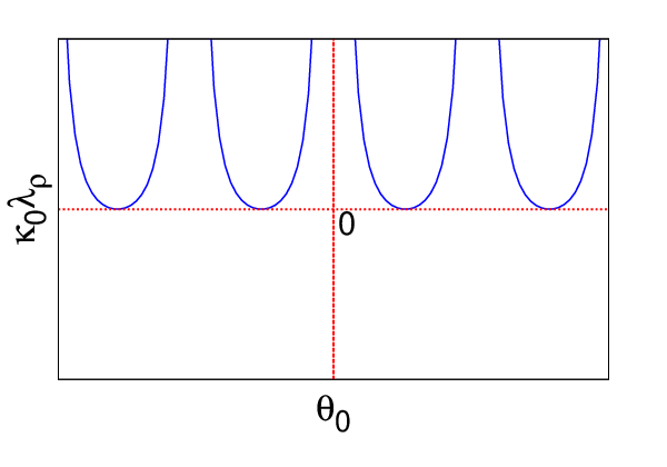
Consider the case when there are only propagating modes at at, say, . Now assume very close to ; we write , where is very small. In that case , up to order . The eigenvalues corresponding to are given by
| (42) |
Noting that is fully imaginary, (42) shows that has real parts, whose signs depend on for a given . Thus, we conclude that the system shows instability for either sign of along with generic propagating modes with an anisotropic wave speed proportional to . Considering in the plane, we thus notice that there are special directions given by along which (small) perturbations move as waves without any growth or damping (to the linear order in ), provided is satisfied; see Fig. 8. Additional values of for which for which the real parts of or vanish may be found from (38). However, both the real parts will not vanish simultaneously at these angles; see Fig. 3. Along all other directions, at least one of should have a real part, and hence perturbations will grow/decay and move. If , there are no special directions with only propagating modes.

Since, and depend on and for all , hence, the two eigenmodes for all , and show generic moving instabilities at for both signs of for arbitrary choice for the active coefficients. It is also clear that at , the system can be stable only if and . Thus, the active stresses clearly distablise the system. Of course, at higher order in , the system will be stabilised by large enough or .
It is useful to analyse the stability of the system for some particular values of . First we start with . In this limit the eigenvalues are given by
| (43) |
Thus there are two modes; one is purely imaginary and hence just a propagating mode, the other has both real and imaginary parts. The sign of the real part is determined by . Thus this eigenvalue is moving and either growing (unstable) or decaying (stable) in time, respectively, when , or, .
For , the stability eigenvalues are given by
| (44) |
From Eq. (44), we note that for , the system is unstable for both and . Next, for and ,
- •
If and , the modes are unstable and oppositely moving.
- •
However, when with , both the modes are unstable. There are no propagating waves.
In the special case with in Eq. (38), i.e., if we ignore the density dependences of the active coefficients, the eigenvalues of the stability matrix take a simpler form
| (45) |
which indicates the presence of propagating modes and instability for both signs of above or below .
Now briefly consider the instabilities with (weak nonequilibrium partial pressure): Neglecting in comparison with , the eigenvalues are given by
| (46) | |||||
Thus, are no longer homogeneous functions of . In order to progress further, assume a ”small” . Then, in an expansion in powers of , we obtain to the lowest order in and
| (47) | |||||
| (48) |
Thus, in the former case, we find instabilities for either sign of , where as in the second case, we find oppositely moving propagating waves.
III.2 Intermediate friction
We again consider first.To the lowest order (linear order) in , the eigenvalues of the linear stability matrix are
| (49) | |||||
which are independent of . We can make the following general conclusions about the mode structures from (49). First of all, none of the active stress coefficients and appear in (49). Thus the active stress is irrelevant in the dynamics to the linear order in . The dynamics at this order in is controlled by the remaining active coefficients, viz, and . This is clearly in contrast to the situation with large . Secondly, if , then the discriminant is positive for all values of to the linear order in . Then only propagating modes will be present for all values of . As before, there should be two oppositely moving propagating modes with the speed of wave being anisotropic and proportional to . If on the other hand , the discriminant in (49) is negative for all magnitudes of at least at , giving rise to instability in the system for both signs of . These instabilities are moving in the opposite directions. In general, for any value of satisfying and for both signs of , both the modes are propagating without damping (or growth). Thus, any perturbation in a region of the polar plane satisfying the above condition moves without any growth or decay in the amplitude (up to ). Else, in the remaining region of the polar plane, one of the modes is unstable and the other stable. The speed of the moving stabilities are unsurprisingly anisotropic and proportional to . The above consideration for allows us to define an angle such that
| (50) |
Then, for in the shaded region in Fig. 9 characterised by there are only propagating waves at , outside of this region, the system is linearly unstable at .

The growth rate or relaxation rates of the unstable and stable modes are also anisotropic and scale with . Representative plots of the real and imaginary parts of as functions of for some chosen parameter values are shown in Fig. (10) showing the presence of propagating modes. The regions of instabilities and propagating modes are clearly indicated. In particular, there are a few notable features as displayed by Fig. 10, consistent with the forms of the eigenvalues (49). For instance, for , are wholly imaginary for all and unequal, i.e., the speed of the two modes are different in magnitude. In contrast, for , the real parts vanish over an identical range of for both the modes, that belongs to the shaded region in Fig. 9, with unequal imaginary parts, i.e., different speeds for the two modes. For the other values of , the real parts are nonzero with mutually opposite signs, representing stable and unstable modes, with same speeds of propagation. The overall differences with the eigenvalues for large (diverging) are clearly visible.

, 
 ,
, 
Evidently, the model is overall stable at the linear order in , provided, . In this stable sector of the parameter space, the results of Ref. [6] that includes the effects of the nonlinearities and noises should directly apply here. Lastly, dry active matters are characterised by density segregation in the steady states [43, 44]. Our linearised treatment is unable to capture this.
III.3 Weak friction limit
We now analyse the linear instabilities for . One of the eigenvalues of the linear stability matrix is non-zero at . We find
| (52) |
With a given choice for the sign of (say positive), for and having the same (opposite) signs and vice versa for , suggesting instabilities for either sign of . These results are identical to those in Ref. [9] for a bulk polar ordered active fluid. It is not a surprise that our results are same as those in Ref. [9], for in the weak limit, the active fluid layer in our model is effectively dynamically decoupled from the ambient fluid and hence acts as a free standing system, and hence, identical to the system considered in Ref. [9].
IV Linear instabilities and measurements of
As our results above reveal, the magnitude of delineates different regimes of the model. While all these regimes display generic long wavelength instabilities in the different regions of the parameter space, the detailed nature of the instabilities and the regions in the parameter space where they are present, vary depending on . For easy comparison, we provide here a table (Table 1) which differentiates between the instabilities in the three different regimes, as delineated by (assume ):
| High friction () | Intermediate friction () | Weak friction [] |
|---|---|---|
| Eigenvalues vanish at . | Again eigenvalues vanish at . | Nonzero eigenvalues: generic linear instabilities for at for both signs of ; no propagating modes. |
| : Generically linearly unstable at for both signs of . In the plane at an angle (measured with respect to the direction of the reference orientation) given by for , or, for and : only propagating modes at . Else instability even at . | : Only propagating modes for . Else, for , there are only propagating modes without any damping or growth for angles in the plane satisfying and instability elsewhere in the plane. | - |
Despite the loose similarities between the nature of the long wavelength instabilities for large and moderate , closer inspection reveals significant differences between the two cases. With a large (formally diverging) , the active fluid velocities , where as, for moderate , . Furthermore, with a diverging , the system is unstable in the full parameter space to the lowest order in along all angles in the polar plane, except for along the lines . Along these special directions, there are only propagating modes without any damping or growth (to the linear order in ). At every other value of , one mode is unstable. Thus, for all (finite) values of the parameters and both signs of , there are moving instabilities with anisotropic speeds. In contrast, with intermediate interfacial friction (), there are regions in the parameter space where there are only propagating modes with no instabilities at the lowest order in for any ; only in a subspace of the parameter space, one encounters moving instabilities for either sign of . Even in such a parameter subspace, there are only propagating modes at for a range of ; for other values of , moving instabilities are present.
At this stage, it is useful to compare with available experimental results. To do this, numerical estimates of the slip length or the slip coefficient are needed. To our knowledge, systematic measurements of or for active fluids are lacking. Nonetheless, based on the available information we can make the following comments. Ref. [24] reports a hydrodynamic length to be of the order of 10 . Assuming and [45] as the thickness of actin cortex, we find , larger than the typical size of cortical action layers (). Nevertheless, our estimation of is not precise and hence it is difficult to comment upon the experimental realisability of the high friction case of in-vitro cortical actin layers in water based upon our estimates. On the other hand, smaller than should correspond to the intermediate friction case; we expect this to be realised in experiments on cortical actin layers in water. Lastly, for , which is certainly small, the system should behave as a free standing system. Equivalently, for a larger system with , the dynamics of a free standing film will be observed if the system is probed at length scales much smaller than ; see, e.g., Ref. [24]. The sensitive dependences of the long wavelength dynamics of the model on may be used to make experimental estimates of in a given system (i.e., for a fixed values of all other parameters including ). We note that directly connecting our theoretical predictions with experimental results is not an easy task. Nonetheless, given the generic nature of our continuum active fluid theories and noting that since an experiment is necessarily performed on finite systems, long wavelength limit should imply , where is a wavevector of interest and the system size, it is expected that all experiments that may be described by the same long wavelength continuum equations should display similar long wavelength linear instabilities, characterised by their growth rates or thresholds of the linear instabilities. In general, these properties should allow us to compare the theoretical predictions with experiments, at least qualitatively, although varying experimentally is expected to be a challenging task. More specifically, we can make the following comments. First of all, if linear instabilities are found to persist for all , then our above results indicate that or a large : , hence, , setting a lower bound for . On the other hand, if linear instabilities are not found at or found only over a range of , we can conclude , or, , giving an upper bound on . At the same time, we must have , yielding , where is a small scale ( molecular cut off), such that for , the continuum theory breaks down. This provides a lower limit on . In contrast, the system behaves as a free standing 2D film for . Information on may also be obtained by measuring the correlation functions of the local velocity fields, orientation and density fluctuations and using the relations (32) and (33) when the system is stable with an intermediate , i.e., with . Velocity fields may be measured, e.g., by attaching a small bead with the actin filament and tracking its instantaneous positions. Orientation and density fluctuations may be measured by optical methods and scattering experiments, respectively. Lastly, as we have shown in Appendices (D.1), (D.2) and (D.3) that the magnitude of bulk 3D fluid velocity depends strongly on for . Thus, measurement of the ambient 3D velocity field, e.g., by tracking the position of a tracer particle, should also be helpful in extracting numerical estimates on .
V Nematic limit of the dynamics
Until now we have considered polar active particles, so that the corresponding dynamics is not invariant under . In the nematic limit, the dynamics is invariant under . Hence, active coefficients and and equilibrium couplings and are zero. Thus, to the lowest order, the dynamical equations in the strong friction case are
| (53) | |||||
| (54) |
As before, assume a time dependence of the form for the fluctuations. Then, to the lowest order in
| (55) |
Thus, with positive , is positive (negative) for and having the same (opposite) signs. Similarly for . Thus, the system is unstable for both signs of .
For a finite , to the lowest order in , the corresponding dynamical equations with nematic symmetry are
| (56) | |||||
| (57) |
Interestingly, Eqs. (56) and (57) are identical to those in Ref. [10] for active nematics on a substrate. Thus, the results of Ref. [10] are to hold here. We do not discuss these here in details. Regardless of the details, in the nematic limit there are no propagating waves and the instabilities are always static or localised. In contrast, active polar ordered systems are characterised by the presence of generic propagating modes and moving instabilities. Finally, the eigenmodes in both the nematic and polar ordered systems with strong interfacial friction with the embedding fluid scale with . However, for intermediate friction, the eigenmodes for the nematic system scale as , where as for the corresponding polar ordered system, they scale as .
VI Summary
In this work, we have set up the generic coarse-grained dynamics of a thin layer of polar ordered active particle suspensions frictionally coupled to the bulk isotropic passive fluid with an arbitrary friction coefficient . In a linearised treatment for small fluctuations around uniformly polar ordered states, we show that our model describes a layer of wet active matter, dry active matter and a free standing film, respectively, for , and . The nature and the conditions for linear instabilities in the long wavelength limit depend sensitively on . These features may be used to find estimates about in a given 2D active fluid layer embedded in a bulk passive fluid. We also discuss the nematic limit of the dynamics and compare it with their polar analogues.
Our results evidently highlight the crucial role played by the interfacial friction and demonstrate how experimental knowledge about the linear instabilities may be used to extract information about the friction coefficient. Actual biological realisations of quasi-2D active fluids have more complicated structures. Our work should be considered only as a first step towards a more complete physical understanding of such systems. We expect our results to be useful in understanding in-vitro experiments on reconstituted layers of ordered actin filaments with molecular motors in an embedding fluid (e.g., water). Experimental validation of the -dependences of the linear instabilities are expected to be highly challenging tasks. Nevertheless, we look forward to possible experimental attempts to study the issues highlighted here. Lastly the formal similarities between the dynamical equations with moderate interfacial friction and those for a polar ordered system resting on a solid substrate open up the possibilities of studying the physics of moderate friction by performing experiments on an analogous system resting on a solid substrate.
Our analyses are valid for small fluctuations around an ordered state. Thus no conclusions may be drawn from our studies about the eventual steady states in the event of the linearly unstable uniform initial states. Numerical solutions of the full model equations should yield valuable information in this regard. We made several simplifying assumptions while setting up our framework. For instance, we have assumed the active fluid layer to be inflexible and hence the out-of-plane fluctuations are prohibited. However, this condition may be violated for reconstituted actin filaments on a liposome. Thus for better quantitative understanding of the experimental results, a thin layer of active fluid with finite flexibility (i.e., with a finite surface tension or bending modulus) should be studied. Secondly, the system may not even be overall flat and may have a finite curvature. In this case, our results should hold over scales smaller than the radius of curvature. Our assumption of equal friction coefficients on both the sides of the active system is also a simplification. Generalisation to unequal frictions on both sides may be done in a straightforward way. It will be interesting to study the diffusivity of a test particle inside the 2D active polar system. It is well-known that the diffusivity of a test particle in a free standing thin active fluid layer shows starkly unusual properties, e.g., dependences on the thickness [46], in contrast to the diffusivity of a small particle in a quasi-2D passive fluid [47]. Given our results here, it is expected that the diffusivity of a test particle in a 2D polar ordered medium is affected by the interplay of hydrodynamic interactions by the embedding medium and the strength of the interfacial friction.
VII Acknowledgement
We would like to thank Jean-Francois Joanny, John Toner, Jacques Prost and Arnab Saha for discussions at various stages of this work, and Frank Jülicher for critical comments on the manuscript. NS would like to thank Krishanu Roy Chowdhury for helpful suggestions with plotting. One of the authors (AB) wishes to thank the Max-Planck-Gesellschaft (Germany) and the Department of Science and Technology/Indo-German Science and Technology Centre (India) for partial financial support through the Partner Group programme (2009).
Appendix A Derivation of the full 2D generalised Stokes equation for
Here, we derive the full 2D generalised Stokes equation. Using Eqs. (7), (10) in Eq. (5), the generalised Stokes Eq. may be written as
| (58) |
Using this value of in (58), the Stoke’s equation is derived as
| (60) | |||||
where is the transverse projection operator written as . Let us redefine as given by (6). Linearising about , the Stokes equation (60) is simplified to
| (61) | |||||
Now using Eq. (15), we find . In addition, acts as a Lagrange multiplier to enforce the constraint . Notice that contributes terms which are higher order in gradients in Eq. (61). Thus neglecting all the higher order terms, the generalised Stokes equation up to the lowest order in gradients is given by Eq. (16).
Appendix B for high friction ()
The velocity and hydrodynamic pressure for the subphase and superphase are given by Eqs. (66)-(73). We impose incompressibility on the 3D ambient fluid:
| (62) |
for both and . Fourier transforming the in-plane coordinates ,
| (63) | |||||
| (64) | |||||
| (65) |
where ; is the in-plane Fourier wavevector. The above equations can be solved together to obtain the solutions for , , and . We write
| (66) | |||||
| (67) | |||||
| (68) | |||||
| (69) | |||||
| (70) | |||||
| (71) | |||||
| (72) | |||||
| (73) |
where coefficients are real or imaginary functions of .
The incompressibility condition (62) yields
| (74) | |||||
| (75) |
The continuity of velocity or Eq. (24) gives
| (76) | |||||
| (77) | |||||
| (78) |
As the active fluid film is two dimensional, there is no discontinuity over the vertical gradient of (since ). This allows us to write
| (79) |
which yields using Eqs. (70) and (71)
| (80) |
The tangential stress may be evaluated using the Stokes equation (17). The Stokes equation for yields
| (81) |
Eq. (81) gives us further relations
| (82) | |||||
| (83) |
Using Eqs. (74)-(78), (80), (82) and (83), the -component of 3D force is obtained as
| (84) | |||||
where we have used incompressibility of the 3D velocity in the last line. Similarly we get the -component of as
| (85) |
using the no-slip condition equating with the in-plane components of at the active fluid layer.
Appendix C Form of for intermediate friction ()
We start with
| (86) |
A similar condition exists at . Now using the forms of and as given by (66), (68) and (70) we obtain
| (87) | |||
| (88) |
In the weak friction limit, in the wavevector range of interest. Thus,
| (89) | |||
| (90) |
or, equivalently,
| (91) | |||
| (92) |
at . Similar considerations at finally yields
| (93) |
This yields for the 2D generalised Stokes equation which satisfy
| (94) |
Now write Eq. (94) in the Fourier space and neglect assuming . This yields Eqs. (32) and (33).
Appendix D Velocity profiles of the ambient fluid
It is instructive to obtain the flow profiles of three-dimensional velocity fields, that are created by the (small) fluctuations in and , in the three different regimes of our model as delineated by the values of .
D.1 Large
In this case . Since , from (70) and (71), . Using the no-slip condition on and the 3D incompressibility of , in the Fourier space. This yields . Thus, everywhere above and below the active fluid layer. Hence, the flow in the surrounding fluid is actually 2D, parallel to the active fluid layer. We further find and . Thus in the Fourier space,
| (95) | |||||
Therefore, has the same form as with an exponentially damped amplitude by a factor and hence shows the same instabilities at .
D.2 Intermediate
In the intermediate friction case, the 3D shear stress balance is given by
| (96) | |||||
| (97) |
Using the above equations and (66), (67), (68) and (69), we get a set of relations between the couplings given by
| (98) | |||||
| (99) | |||||
| (100) | |||||
| (101) |
Now using (98), (99), (100), (101), 3D incompressibility () of ambient fluid, 2D incompressibility () of active fluid layer and equations (82) and (83), we can show that
| (102) | |||||
| (103) |
Hence we obtain, for all identically and and has the same dependences on and as for large . Thus, is again 2D. Nonetheless, for moderate is different from for large , since the solutions for and have very different explicit forms for moderate . In particular, shows instability only if , the same condition for instability for the 2D active fluid layer. Notice that in the present case in addition to the factors, is further scaled down in comparison with by a factor , and hence should be small in magnitude.
D.3 Small
In the limit of very small , we have . i.e., we effectively have the stress-free boundary condition on at . In addition, at . Now using the results in Sec. C, we find , i.e., at all and identically. In addition, everywhere. Thus, the 3D velocity field vanishes.
References
- [1] T. Butt et al., J. Biol. Chem. 285, 4964 (2010); V. Schaller et al., Nature 467, 73 (2010); V. Schaller, C. Weber, E. Frey, and A. R. Bausch, Soft Matter 7, 3213 (2011); Y. Sumino et al., Nature 483, 448 (2012); H. P. Zhang, A. Be’er, E.-L. Florin, and H. L. Swinney, Proc. Natl. Acad. Sci. USA 107, 13626 (2010).
- [2] S. Ramaswamy, Annu. Rev. Condens. Matter Phys. 1, 323 (2010).
- [3] T. Surrey, F. J. Ned́eĺec, S. Leibler, and E. Karsenti (2001), Science 292, 1167.
- [4] C. Dombrowski, L. Cisneros, S. Chatkaew, R. E. Goldstein, and J. O. Kessler, Phys. Rev. Lett. 93, 098103 (2004).
- [5] R. Kemkemer, D. Kling, D. Kaufmann, and H. Gruler, Eur. Phys. J. E 1, 215 (2000).
- [6] J. Toner and Y. Tu, Phys. Rev. E 58, 4828 (1998).
- [7] V. Narayan, N. Menon and S. Ramaswamy, J. Stat. Mech., P01005 (2006); V. Narayan, S. Ramaswamy, and N. Menon, Science 317 (5834), 105 (2007).
- [8] W. F. Paxton, K. C. Kistler, C. C. Olmeda, A. Sen, S. K. S. Angelo, Y. Cao, T. E. Mallouk, P. E. Lammert, and V. H. Crespi, J. Am. Chem. Soc. 126, 13424 (2004).
- [9] R. A. Simha and S. Ramaswamy, Phys. Rev. Lett. 89 058101 (2002).
- [10] S. Ramaswamy, R. A. Simha, and J. Toner, Europhys. Lett. 62, 196 (2003).
- [11] V Schaller, C Weber, C Semmrich, E Frey, AR Bausch, Nature 467, 73 (2010).
- [12] P. C. Martin, O. Parodi, and P. S. Pershan Phys. Rev. A 6, 2401 (1972).
- [13] I. S. Aranson and L. S. Tsimring, Granular Patterns (Oxford University press, New-York, 2009), Chap. 9.
- [14] K. Kruse, J.F. Joanny, F. Jülicher, J. Prost, K. Sekimoto, Eur. Phys. J. E 16, 5 (2005).
- [15] T. Vicsek and A. Zafeiris, Phys. Rep. 517, 71 (2012).
- [16] M. C. Marchetti, J. F. Joanny, S. Ramaswamy, T. B. Liverpool, J. Prost, Madan Rao, and R. Aditi Simha Rev. Mod. Phys. 85, 1143 (2013).
- [17] J.-F. Joanny, J. Prost, in Biological Physics, Poincare Seminar 2009, edited by B. Duplantier, V. Rivasseau (Springer, 2009) pp. 1-32.
- [18] A. Maitra, P. Srivastava, M. Rao and S. Ramaswamy, Phys. Rev. Lett. 112, 258101 (2014).
- [19] R. Voituriez, J.-F. Joanny and J. Prost, Euro. Phys. Lett., 70, 404 (2005).
- [20] S. Mishra and S. Ramaswamy, Phys. Rev. Lett. 87, 906202 (2006).
- [21] The thin active fluid layer in our model corresponds to the cortical actin layer in a cell, where as the embedding fluid in our model represents the bulk cytoplasm. While these straight forward relations between our model and the cell cortex seem self-evident and simple, it should be remembered that in an eukaryotic cell, there are no sharp bloundaries between the cortical actin layer and the bulk cytoplasm. In addition, the bulk cytoplasm is not a passive fluid; it has active processes going on in it.
- [22] B. Alberts, D. Bray, J. Lewis, M. Raff, K. Roberts, J.D. Watson, Molecular Biology of the Cell, 3rd edition (Garland, New York, 1994).
- [23] L.-L. Pontani et al, Biophys J. 96, 192 (2009).
- [24] A. Saha, M. Nishikawa, M. Behrndt, C.-P. Heisenberg, F. Jülicher, S. W. Grill, arXiv:1507.00511.
- [25] J. F. Joanny, F. Jülicher, K. Kruse and J. Prost, NJP 9, 422 (2007).
- [26] See also A. C. Callan-Jones and F. Jülicher, NJP 13, 093207 (2011) for a slightly different formulation for a multicomponent active fluid.
- [27] P.-G. de Gennes, J. Prost, The Physics of Liquid Crystals (Clarendon, Oxford, 1993).
- [28] Y. Zhu and S. Granick, Phys. Rev. Lett. 88, 106102 (2002).
- [29] Y. Zhu and S. Granick, Langmuir 18, 10058 (2002).
- [30] R. Zhao and C. W. Macosko, J. Rheol. 46, 145 (2002).
- [31] Y. C. Lam, et al., J. Rheol. 47, 795 (2003).
- [32] Q. Ehlinger, L. Joly and O. Pierre-Louis, Phys. Rev. Lett. 110, 104504 (2013).
- [33] K Kruse, J F Joanny, F Jülicher and J Prost, Phys. Biol. 3, 130 (2006).
- [34] G. Salbreux, J. Prost,1,2 and J. F. Joanny, Phys. Rev. Lett. 103, 058102 (2009).
- [35] J.-Y. Tinevez et al, Proc. Nat. Acad. Sc. (USA) 106, 18581 (2009).
- [36] M. Mayer, M Depken, J. S. Bois, F. Jülicher and S. W. Grill, Nature 467, 617 (2010).
- [37] A Doostmohammadi, M Adamer, S P Thampi and J M Yeomans, arXiv:1505.04199.
- [38] A Ward et al, Nature Mat. Lett. 14, 583 (2015).
- [39] H. Chaté, F. Ginelli, G. Grégoire and Franck Raynaud Phys. Rev. E 77, 046113 (2008).
- [40] E. Bertin, M. Droz and G. Grégoire, arXiv: 0907.4688 (2009).
- [41] F Thüroff, C Weber, E Frey, Phys. Rev. X 4, 041030 (2014).
- [42] D.K. Lubensky and R.E. Goldstein, Phys. Fluids 8, 843 (1996).
- [43] E. Bertin et al, NJP 15, 085032 (2013).
- [44] S. Ngo et al, arXiv:1312.1076.
- [45] A. G. Clark, K. Dierkes and E. K. Paluch, Biophys. J. 105, 570 (2013).
- [46] A. Basu, J.-F. Joanny, F. Jülicher and J. Prost, New Journal of Physics 14, 115001 (2012).
- [47] P. G. Saffman and M. Delbrück, Proc. Nat. Acad. Sc. (USA) 72, 3111 (1975).