Breakdown of Kinetic Compensation Effect in Physical Desorption
Abstract
The kinetic compensation effect (KCE), observed in many fields of science, is the systematic variation in the apparent magnitudes of the Arrhenius parameters , the energy of activation, and , the preexponential factor, as a response to perturbations. If, in a series of closely related activated processes, these parameters exhibit a strong linear correlation, it is expected that an isokinetic relation will occur, then the rates become the same at a common compensation temperature . The reality of these two phenomena continues to be debated as they have not been explicitly demonstrated and their physical origins remain poorly understood. Using kinetic Monte Carlo simulations on a model interface, we explore how site and adsorbate interactions influence the Arrhenius parameters during a typical desorption process. We find that their transient variations result in a net partial compensation, due to the variations in the prefactor not being large enough to completely offset those in , both in plots that exhibit a high degree of linearity and in curved non-Arrhenius plots. In addition, the observed isokinetic relation arises due to a transition to a non-interacting regime, and not due to compensation between and . We expect our results to provide a deeper insight into the microscopic events that originate compensation effects and isokinetic relations in our system, and in other fields where these effects have been reported.
pacs
PACS numbers: 82.20.Db, 68.43.Vx, 68.43.Nr, 68.43.DeI Introduction
Many physical, biological, and chemical processes exhibit a strong temperature dependence, in the sense that they rely on thermally activated mechanisms to overcome energy barriers in order for the process to proceed. The rate, , of many such processes follows an Arrhenius type behavior:
| (1) |
where is the activation energy, the preexponential factor, is the temperature and is Boltzmann’s constant. Information parameterizing such processes are usually obtained through an Arrhenius plot, constructed with a series of measurements of vs. , from which one obtains the activation energy as the slope, and the preexponential factor from the intercept.
A characteristic feature in a series of closely related thermally activated processes, where a parameter has been varied (e.g. the concentration of an additive in a chemical reaction) is a systematic change in the apparent magnitudes of and [1, 2, 3] as a response to perturbations, known as the kinetic compensation effect. Such a hypothetical set is schematically represented in Fig. 1.

The premise behind the concept of ‘compensation’ is that a change in the magnitude of is compensated or offset by a concomitant change in the preexponential factor [3, 4, 5, 6, 2], and they satisfy the linear relationship [7, 5]:
| (2) |
where and are constants. This linear relationship originates from the Constable plot, which is, in turn, contructed with the data pairs obtained from the slope and intercept, respectively, of the Arrhenius plot [8, 9, 1]. A hypothetical Constable plot of vs. is schematically represented in Fig. 2.
Following this method of analysis, a kinetic compensation effect is observed when the data points on the Constable plot fall on a straight line [10]. Then the parameters are obtained by combining Eq. 2 with Eq. 1: ; then becomes , where is the compensation temperature [1, 8, 3, 7], and becomes . This predicts that at the Arrhenius plots cross, and at that point the rates become the same and ‘independent of external parameters and perturbations’ [10, 11, 7, 1, 12]. This is known as the isokinetic relation (IKR) [10, 1], or isokinetic equilibrium, also schematically represented in Fig. 1. Historically, the KCE and IKR have been defined interchangeably or as synonymous [13], since the observation of one is thought to directly imply the occurrence of the other [1, 13]. This is a natural assumption, given that, as seen before, one can predict the IKR from a the linear relationship in Eq. 2. We should note, however, that this is only possible when the linear correlation coefficient between data points in the Constable plot is exactly [1].
In their extensive review [1], Liu and Guo propose that the KCE and IKR are separate phenomena, which may be observed independently, and should be characterized as such: the KCE should be identified solely by the strong linear correlation between and [5, 1, 10, 8, 14, 12], and the IKR by the convergence of Arrhenius plots around a single temperature value [1, 12].

The extraction of parameters from the slope and intercept of an Arrhenius plot has proven to be a useful and important method that allows for the empirical determination of rates [15, 13], however, it has been widely accepted for some time now that the parameters and need not be constants throughout many activated processes [16, 17, 5, 18, 19, 20, 21]. This leads to the observation that each point in the Constable plot indeed corresponds to a data pair of fixed values of , therefore, if the two phenomena are to be defined separately, this raises the question of the physicochemical significance of an observed linear correlation in a case where the IKR is not simultaneously satisfied.
It has been proposed that throughout an activated process the parameters vary in a manner such that they increase or decrease in the same direction, and compensate or offset each other, in a way that the overall rate remains almost unchanged [21, 17, 9, 4, 1, 2, 11, 6, 3, 20, 22, 5]. This behavior would perhaps justify the extraction of constant Arrhenius parameters, but has not been explicitly demonstrated[23, 24, 1]. A strong interdependence of the parameters has been attributed to them being extracted from the same temperature dependent data [1, 10, 25], instead of through independent measurements (which are not always possible). A strong linear correlation obtained this way is likely, as mentioned by Cornish-Bowden in [25], the consequence of the two variables being ‘larguely the same variable looked at in two ways’. In addition, some instances of the IKR do not yield a compensation temperature that falls within the experimental range, and is therefore found by extrapolation [3, 25]. Thus the existence of the kinetic compensation effect and isokinetic relation continue to be the subject of heated debate, and are often believed to have a purely mathematical origin [26, 15, 10, 8, 25] and to lack any physical or chemical significance.
Nevetheless, the KCE and IKR, as well as the closely related entropy-enthalpy compensation, continue to be reported in many different areas of science, such as temperature programmed desorption [23], fouling [15], grain boundary migration [9], heterogeneous catalysis [2], crystallization of amorphous solids [27], glass transitions [28], adsorption [29, 30, 7], chemical reactions [7] molecular self-assembly [11, 31] and the melting of solids [22] among others.
Here, we explore the very notion of the KCE, at the fundamental level, through the use of kinetic Monte Carlo [32] simulations in the context of physical desorption; to do this we quantify the transient variations in the Arrhenius parameters throughout the activated process and verify if those changes exhibit a compensatory behavior. Our methodology is to perform the ab initio numerical calculation of the energy of activation, along with the calculation of the decrease in the coverage with increasing temperature, during the thermal desorption of interacting and non-interacting adsorbates from an energetically homogeneous, crystalline lattice. By doing this we step aside from an approach that relies on preconceived functional forms that yield the best fit to the desorption data [6, 10], and/or that predicts the variations in the parameters to yield a KCE and an IKR, in the context of the criteria used to identify them in [1]. In the present work we consider only attractive lateral interactions. Using our numerical results for and coverage, we can extract the preexponential factor , and quantify its transient variations as well. To our knowledge, this approach has not been done before.
Our numerical results span a range of adsorbate-adsorbate attractive interaction strengths, calculated as a percentage of the fixed surface binding energy, this provides the experimental parameter that is being altered in the series of similar activated processes; all while keeping the substrate structure fixed. Our method allows us to verify and explicitly quantify the level of compensation that has not been successfully achieved to date using more traditional methods. Snapshots of our computer simulations are shown in Fig. 3.
Our results show that the parameters effectively exhibit a behavior that supports the occurrence a compensation effect, however, the observed changes in the preexponential factor are not large enough to effectively compensate or offset the significant variations in the activation energy, , which arise due to strong coverage dependence. This produces a net partial compensation between and in all regimes of interaction strength presented in this study. These results are in stark contrast with previously reported strong coverage dependencies of the preexponential factor in the regime of strong interactions [17, 20, 19], which can result when the parameters are extracted through forced linearization [24, 23, 17]. Partial compensation has been previously considered [1, 3], but this notion is not as widespread as that of a complete KCE; here we also observe that the partial compensation effect is not incompatible with the occurrence of curved Arrhenius plots, also referred to as non-Arrhenius behavior [21, 18, 33, 34].
In the context of isokinetic equilibrium, we observe a tendency of the Arrhenius plots to converge towards the region of low coverage and high temperature. Our plots, however did not cross at a common , instead the interacting regime plots reach the non-interacting one at significantly different temperatures, which could be due to the difference between regimes of interaction strength. Nevertheless, we extracted those temperatures, as well as the values of and at those points, and found that the Arrhenius parameters become numerically very close to those assigned to the bare surface, which implies that the convergence of rates cannot be attributed to a compensation effect between and , but instead to a transition to a regime where the effects of lateral interactions become negligible. And it is also consistent with the rates becoming independent of perturbing parameters.
We also analyzed a subset of data with adsorbate-adsorbate interaction strenght of of the binding energy of the surface. Many physisorption experiments with weakly interacting adsorbates and energetically heterogenous, crystalline surfaces fall in this category [35]. We performed the linear fit to the Arrhenius plots and show that the slope and intercept method of analysis yields more accurate results in this regime, and also that, in this regime, the assumption of a constant preexponential factor can be justified. Nevertheless, the parameters exhibit the same behavior we observed in the other stronger interaction regimes, as well as the tendency towards an IKR, which can also be explained in terms of a transition to the non-interacting regime.


II Model system and Methodology
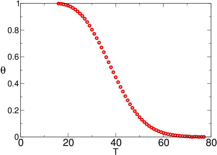
TPD is an experimental technique used in surface science to extract surface parameters, such as binding energies, sample porosity [36] and sorption capacity; it has applications in chemical speciation [37] and contaminant removal [38]. In a typical experiment a surface in an evacuated chamber is exposed to a gas until the desired uptake is achieved, then the sample is heated with a linear temperature ramp of the form: , where is the temperature step and is time. The results are in the form of the substrate fractional coverage, , as a function of temperature [39]. A typical simulation data set is shown in Fig. 4 for the non-interacting species examples shown in Fig. 3. The corresponding rate and Arrhenius plots are shown in in Fig. 5.
The most common method of analysis starts with the Polanyi-Wigner equation of desorption:
| (3) |
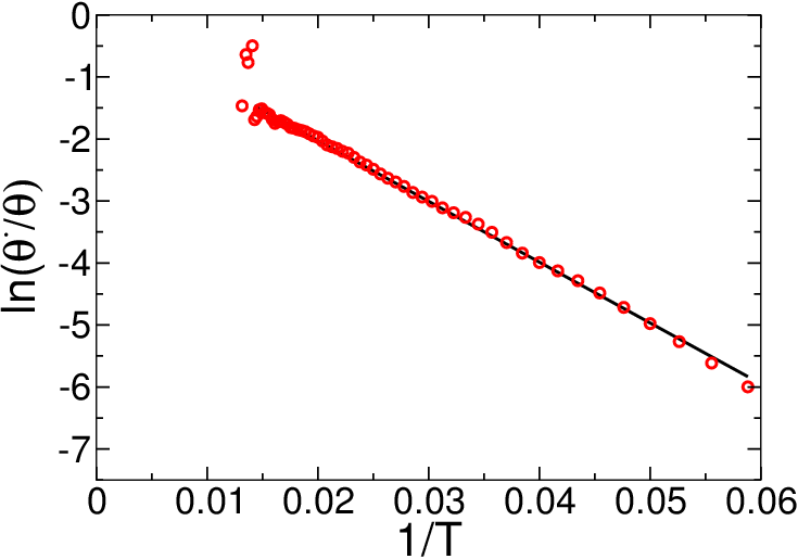
where, is the rate at which the coverage decreases with increasing temperature, and the order of the process. Physical desorption from a uniform planar surface corresponds to order , thus we set for the remainder of the present work. The most common method of extraction of the parameters of interest is from the slope and intercept, respectively, of the Arrhenius plot, vs. , where in our case, (see Fig. 5). As discussed before, such a parameterization has proven useful in the empirical determination of rates [15], however, the parameters and exhibit variations throughout the desorption process due to one or more of the following factors: surface energetic heterogeneity [40, 41], lateral interactions [23, 24], multiple chemical species [42], and/or changes in surface configuration [4].
Our methodology is to simulate a TPD process from a quasi-two dimensional, square lattice of side , with sites and periodic boundary conditions using a kinetic Monte Carlo algorithm [32]. The lattice is energetically homogeneous, so that each site , has an associated binding energy, , in units where . We explore attractive interaction strengths , that range from to . To track the desorption process, the kinetic Monte Carlo scheme follows a series of steps: we first specify the initial conditions, including the binding and interaction energies, initial temperature (which we alter depending on ), step size, and initial coverage (which is set to in all cases). The second step is to calculate the number of occupied nearest neighbors per site, the site energies, and the probabilities associated with each of the allowed transitions. The energy desorption barrier per site , is given by
| (4) |
where each site, , picks up an energy contribution from its nearest occupied neighbors. Thus, when a neighbor site is occupied, zero if empty, and is the coordination number for the square lattice under consideration here. Next, an allowable transition - desorption or diffusion to a neighboring site - is selected and the state of the system is updated, then the time counter is increased as prescribed by the kinetic Monte Carlo algorithm within the grand canonical ensemble. The temperature ramp is controlled by increasing after so many time steps , which is here set to unity. Finally the coverage, temperature and activation energy are updated and recorded. The process is repeated until the lattice is completely empty. Our results are obtained as an (ensemble) average over 100, independent runs; see Fig. 3 for representative simulation images at early (low), intermediate, and late (high) times (temperatures).

III Results
The first step is to verify that our simulation results can be fitted to Eq. 3 for the non interacting regime ().We show this on the left panel of Fig. 5. On the right panel of the same figure, we performed the corresponding linear fit to the Arrhenius plot, from which we obtain the following parameters: and (extrapolated intercept). The value for , as expected, matches the input binding energy, , within error.


III.1 Activation Energy
One of our main results is the calculation of the transient variations in the energy of activation throughout the desorption process, during which is calculated using Eq. 4 as, .
Our results for are plotted as a function of coverage in Fig. 7. In the non-interacting regime, the activation energy remains constant and matches the binding energy itself, as expected, which is consistent with the fact that it represents the only energy barrier to desorption. This feature of the non-interacting regime also applies locally at each site. In the case of interacting species, on the other hand, additional contributions coming from site-occupied nearest neighbors result in a stronger binding of the adsorbates to the surface, which varies locally due to the heterogeneous distribution of interacting occupied sites throughout the desorption process. This leads to an enhanced activation energy, or effective desorption barrier, and also to the curvature of Arrhenius plots, which is observed to increase as a function of for attractive interactions.

In a MF way, the additional contributions to the activation energy due to occupied sites interacting with occupied neighbors is given by the term: , where is the coordination of the lattice substrate ( for the square lattice used here), is the coverage, and the adsorbate-adsorbate interaction energy. Then, the total mean activation energy is, , where , is the fractional interaction energy. This analysis is shown by the solid line fits to the data in Fig. 7. As seen, the MF approach is only correct for the non-interacting regime (when ) and for the interacting systems only at the extreme coverage values (when and ). The reason behind this is that the MF approach presupposes that at the molecular level, each site sees the same number of occupied neighbors throughout the substrate; in other words the coordination of occupied interacting sites, , is delta-function distributed. This is only true at complete coverage, where the distribution of interacting sites, , and again at zero coverage: . Thus, deviations from the MF picture come from the distribution of interacting sites during the kinetics. As a result, due to the added energy contributions when interactions are present, the sites become energetically heterogeneous. To illustrate this point, Fig. 8 shows the for one interaction energy at several coverages, which shows how the occupation coordination becomes wider at coverages away from complete and zero coverage.

III.2 Pre-exponential Factor

To verify whether a compensation effect occurs, we calculated the rate of desorption analytically, using the energies of activation in Fig. 7 and Eq. 3, while keeping fixed at . These results are plotted in Fig. 9 (solid lines). We then compared the resulting plots with the desorption rate data, obtained through the numerical derivatives of the desorption curves on the top panel of Fig. 6, and are also plotted in Fig. 9 (symbols). The difference between the two indicates that there must be some variation in the prefactor . We then extracted , these results are plotted in Fig. 10, where it can be seen that the preexponential factor also exhibits variations as the coverage decreases.

In the non-interacting regime, Fig. 10 displays how remains constant at unity (the observed fluctuations are due to the numerical derivatives used to obtain the data). For , exhibits a systematic deviation from the non-interacting value as the strength of the interaction increases. In this sense is the bare desorption rate that is renormalized in the presence of interactions. While the trend towards decreasing with increasing , is consistent with some level of compensation, the changes in are significantly smaller in magnitude compared to those in (see Fig. 7), and are not large enough to effect complete compensation.
To visualize the degree to which the parameters compensate each other, we plotted the separate contributions of and to the Arrhenius curve of various interaction strength regimes, these results are shown in Fig. 11. On the left panel we show the Arrhenius plots calculated by keeping fixed at a value of , and using our numerical results for (solid lines). When compared to the Arrhenius plots obtained directly from the desorption data (symbols), the curvature remains almost unchanged, indicating that the relative contribution due to is small in all regimes of interaction strength.


On the right panel of Fig. 11 we added the we plot vs. , and we see that remains approximately constant and relatively close to in all cases. Our results in Figs. 10 and Fig. 11 do not yield ‘unusually large’ preexponential factors that exhibit a strong coverage dependence in the regime of strong interactions [20, 19, 43, 44], and which have been identified as an indicator of false compensation effects in thermal desorption [24].
III.3 Correlations
A thermodynamic point of view posits that the changes in can be attributed to changes in the entropy [45, 9]. This view is somewhat contained within the Erying-Polanyi equation [46, 47, 3], where is associated with the enthalpy of activation , and has a frequency component, , a temperature dependence, and an entropy component [9],
| (5) |
where, is Planck’s constant. It follows that for the non-interacting case, , the frequency component of is unchanged due to the fact that desorption and diffusion events are unaffected by the presence of nearest neighbors, and the changes in are perhaps sufficiently small in this regime, since the number of available microstates from one state to the next does not change significantly with the desorption or diffusion of a single particle. In Fig. 10 we observe that always starts and ends at, or close to, for all regimes: during the initial and final phases of the desorption process, the entropy is at its lowest, and approaches zero at the very beginning and end. At intermediate times/temperatures the entropy increases due to the number of microstates that now become available. In all cases, , the initial phase of desorption occurs through eating away of the large, percolating, connected cluster of occupied sites. Yet, in the non-interacting case, there is a lack of correlation as to which sites become unoccupied, while with increasing , site occupation is correlated over longer timescales as desorption due to the fact that desorption and diffusion events are slowed down. These enhanced correlations can be quantified through the time autocorrelation function for site occupation: , where is the site occupation number, which takes on the values 0 or 1, and is the time lag over which correlations are measured. The results of Fig. 12 (left) demonstrate that correlations in site occupation become greatly enhanced as increases.


As desorption proceeds, the occupied lattice starts to break up into connected (smaller) island clusters of occupied sites, this has been observed experimentally [48]. The number of clusters reaches a maximum value at a coverage value which both depend on interaction strength as indicated by the data shown in Fig. 12(right). We can interpret these features as follows: for a given value of the coverage, systems with stronger interactions are likely to exist in larger but fewer clusters due to enhanced site correlations that persist to longer times/temperatures. If the number of clusters decreases the entropy is expected to decrease, which is reflected in the value of . The data of Fig. 12 shows that the coverage at which the difference in the number of clusters is largest coincides with the greatest difference in the values, consistent with Fig. 10. And although the numerical difference in the number of clusters of Fig. 12 (right) at first sight appears insignificant, amounting to approximately a difference, this becomes significantly magnified when evaluating the entropy through counting the number of accessible microstates.
III.4 False kinetic compensation effects in Thermal Desorption
In this section we explore a reason for a a false compensation effect in thermal desorption, which is demonstrated by Miller et al. in [23]. Starting from the slope of the Arrhenius plot, when all explicit dependencies are considered [23, 24]:
| (6) |
Here the second order terms contained within the parentheses in produce a non-constant slope and can only be ignored if: (1) the parameters are constant, (2) if measurements are made over a region where the change in the coverage is vanishingly small , or (3) if the second order terms sum to zero, as a special manifestation of the compensation effect. Assuming the latter, the following differential equation results: , and its solution reduces back to Eq. 2 [23]. This approach also suggests that the variations in the parameters occur in the same direction, and with the same, or almost the same magnitude, thus the changes in and during the desorption process are ignored [24], and it also forces a straight line through the data that will likely lead to a false KCE [23, 24]. Our results in Figs. 10 and 11 do not support this assumption. The increasing curvature of the Arrhenius plots in Fig. 6 is the first visible indicator, if the variations in the parameters were effectively in the same direction and with the same or almost the same magnitude, then the plots, at the correct order, should always yield straight lines.
To further emphasize this point we calculated the second order terms in 6 using our numerical data. The results are shown in Fig. 13.


In Fig. 13 the derivative of exhibits much larger variations (left panel) than (right panel). When the terms are added, according to Eq. 6, the result is only zero in the non-interacting case, as expected, otherwise it yields a non-zero, finite contribution, which is plotted in Fig. 14.

It should be noted that the factor attenuates variations in , and, while these second order terms are not particularly large, they yield a finite non-zero contribution (see Fig. 6), that, when ignored, forces a straight line through the data.
III.5 Isokinetic relation (IKR)
In the context of isokinetic equilibrium, it can be seen in Fig. 6 (bottom panel) that the plots exhibit a tendency to converge towards the region of high temperature and low coverage. However, and as previously stated, we do not observe that the plots cross at one value of , but all interacting curves seem to reach the non-interacting one, or an extrapolation of it, at different temperatures. We indicate approximate values of for each interaction regime in Fig. 15, and the numerical values of , and at those temperatures are displayed in table 1.
| Crossing Temp. | ||||
|---|---|---|---|---|
| 10 | 60 | -100.3474 | ||
| 30 | 78 | -100.118027 | ||
| 50 | 89 | -100.64 | ||
| 70 | 104 | -100.319222 | ||
| 90 | 118 | -100.235456 |

As observed, the values of are very close to that assigned to the binding energy of the surface . This information and the observed convergence towards the region of low coverage and high temperature, implies that this resembles an isokinetic relation. We did not rely too heavily on the numerical values of the prefactor , since this parameter remains close to throughout the desorption process (see Fig. 10), and the rates become close, but not exactly the same. Nevertheless, the significance of this IKR is that it does not occur because of a compensation between and , but due to a transition to the non-interacting regime, where the rates are governed solely by the parameters of the surface, and is therefore in agreement with the rates becoming independent of external parameters and perturbations [7].
III.6 Weak Adsorbate Interactions
In this section we show numerical results for the regime of weak lateral interactions, specifically for adsorbate-adsorbate interaction strengths of the binding energy. As mentioned before, some physisorption experimental studies fall in this category, such as the desorption of Xe from a graphite surface [35]. In this regime the Arrhenius plots are fairly close to linear, and estimation of the parameters using the slope and intercept method of analysis are more accurate to within a few percent of the actual calculations (see Table 2).

| max. | linear fit | calculated | linear fit | |
|---|---|---|---|---|
| 0 | 100 | 102 | 0.9899 | 1.0 |
| 1 | 104 | 107 | 1.06 | |
| 5 | 120 | 123 | 1.08 | |
| 9 | 145 | 156 | 2.08 | |
| 10 | 140 | 167 | 2.4 | |
| 30 | 220 | 292 | 8.18 | |
| 90 | 460 | 785 | 121.94 |
In table 2 we tabulate the values of the parameters, and extracted by using traditional methods of analysis vs. our numerically calculated results over our complete range of adsorbate-adsorbate interaction strengths . Specifically, we compare how a linear fitting of the data leads to increasing differences from the exact calculated values. While for weaker interaction energies, the parameters from a linear fit procedure provides reasonably accurate estimates, at stronger interactions deviations grow dramatically.
These results demonstrate how ‘unusually high’ preexponential factors can be obtained from extracting the parameters through enforcing the traditional linear fitting methods in the regime of strong interactions. The large magnitude of the extracted values of in the regimes of and interaction strenght have been attributed to a strong coverage dependence [19, 20, 43, 44], but here we have demonstrated that this is not the case and that it is likely that this issue might be a consequence of forced linearization.
In the context of the IKR, we can see the Arrhenius plots in Fig. 16 overlapping in the region of low coverage and high temperature, towards the end of the desorption process. Using the Arrhenius parameters in table 2, we constructed the Constable plot of vs. in Fig. 17, for the regimes with , and interaction strength.
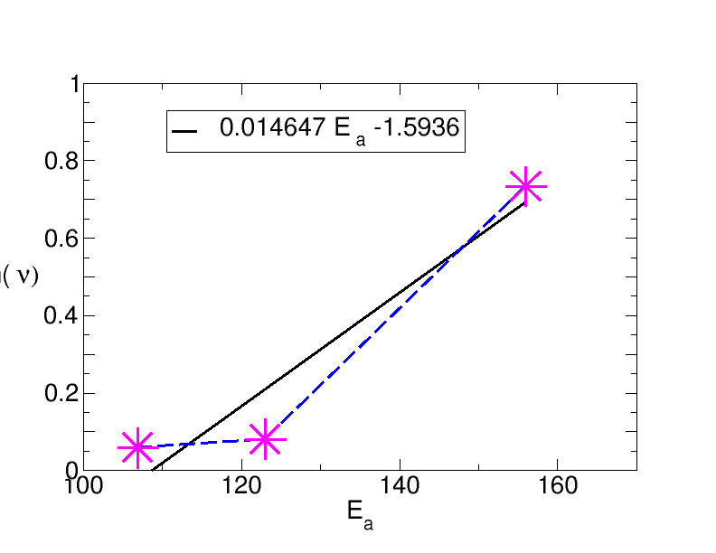
A linear fit to this Constable plot yields a slope with and , with correlation coefficient of . Using , we extracted the values of , and at that point. The results are displayed on table 3, where the numerical values of deviate by a small amount from the surface binding energy , therefore we can consider this to be the point of transition to the non-interacting regime. This point is indicated in Fig. 16. At the Arrhenius plots begin to overlap, and we should point out that henceforth, we can find higher temperature values for which the corresponding values of , and also fall within the non-interacting regime.
The numerically calculated values of at are also close to unity, with some variations. However since the prefactor stays relatively close to throughout the process, we once again rely more strongly on the numerical values of to make this assessment. The values of are also displayed on table 3, and, as can be seen these values are closer to the intercept of the Constable plot. We previously mentioned that for a linear Constable plot to predict an IKR, it is necessary that the linear correlation coefficient is . Here we obtained a strong linear correlation and our analysis yields a compensation temperature in the region where the Arrhenius plots acquire close values of the rate. This demonstrates that, within a regime where molecular interactions are fairly weak compared to the energy of activation, the prediction of the KCE and IKR can be performed using the Constable plot. Nevertheless, the variations in the parameters exhibit the same behavior we observed with stronger interactions. And this implies that compensation effects can occur in non-Arrhenius curves, but cannot be determined using the methods outlined here.
| 1 | 69 | -100.000169 | ||
| 5 | 69 | -100.002511 | ||
| 9 | 69 | -100.01026 |
IV Conclusion
We have demonstrated that the Arrhenius parameters effectively vary in a manner consistent with a kinetic compensation effect. However the variations in the prefactor are not large enough to completely offset those in , and thus a net partial compensation occurs instead. As the interaction strength increases, so does the peak temperature, which is expected, but it also means that the variations in are not sufficient to keep the rates almost unchanged. Although it could be argued that this is due to the relatively large difference between regimes of interaction strenght (here it is ), we observed this same behavior for desorption curves with smaller differences.
A Constable plot in the regime of weak interactions () yields a slope that corresponds to a temperature where the rates acquire close values, but not the exact same, and the Arrhenius plots begin to overlap. This is consistent with the rates becoming independent of external perturbations. We confirmed this by showing that, at this point, the values of and become very close to the bare parameters of the surface. We observed a similar convergence in the stronger interaction regimes ( of the binding energy), however the temperatures at which the rates become independent of adsorbate interactions are considerably different for each Arrhenius plot in this case. Nevertheless, in both instances, the plots tend to overlap because of a transition to a regime where lateral interactions become negligible, and not due to mutual compensation.
The data points on the Constable plot represent the apparent Arrhenius parameters, and although this method of analysis works well within the weak interaction regime, our stronger interaction regime data shows that there can be instances of the KCE in instances where non-Arrhenius behavior is observed, and that these effects may be overlooked due to the strict criteria used to determine the occurrence a KCE and the IKR.
The behavior we observe could very likely help elucidate and compensation effects and isokinetic relations observed in other systems. A better understanding of this phenomenon can help achieve controlled activated events and provide a means to accurately parameterize many biological, chemical and physical processes that share common features in their compensation effects.
Acknowledgements.
N. Zuniga-Hansen and M. M. Calbi acknowledge support provided by the National Science Foundation through grant CBET-1064384. The authors would also like to thank Professor Phillip Sprunger for valuable discussions.References
- [1] L. Liu and Q.-X. Guo, Chem. Rev. 101, 673 (2001).
- [2] B. V. L’vov and A. K. Galwey, International Reviews in Physical Chemistry 32, 515 (2013).
- [3] A. Yelon, E. Sacher and W. Linert, Phys. Chem. Chem. Phys. 14, 8232 (2012).
- [4] P. J. Estrup, E. F. Greene, M. J. Cardillo and J. C. Tully, J. Phys. Chem. 90, 4099 (1986).
- [5] H. J. Kreuzer and N. H. March, Theor. Chim. Acta 74, 339 (1988).
- [6] E. Tomkova and I. Stara, Vacuum 50, 227 (1998).
- [7] K. F. Freed, J .Phys. Chem. B 115, 1689 (2011).
- [8] P. J. Barrie, Phys. Chem. Chem. Phys. 14, 327 (2012a).
- [9] G. Gottstein and L.S. Shvindlerman, Interface Sci. 6, 265 (1998).
- [10] P. J. Barrie, Phys. Chem. Chem. Phys. 14, 318 (2012b).
- [11] J. F. Douglas, J. Dudowicz and K. F. Freed, Phys. Rev. Lett. 103, 135701 (2009).
- [12] W. Linert, Chem. Soc. Rev. 18, 477 (1989).
- [13] R. K. Agrawal, J Therm Anal Calorim 31, 73 (1986).
- [14] V. P. Zhdanov, Surf. Sci. Lett. 12, L662 (1991).
- [15] P. J. Barrie, C. A. Pittas, M. J. Mitchell and D. I. Wilson, Proceedings of International Conference on Heat Exchanger Fouling and Cleaning (2011).
- [16] K. A. Fichthorn and W. H. Weinberg, Langmuir 7, 2539 (1991).
- [17] K. A. Fichthorn and P. G. Balan, J. Chern. Phys. 101, 20028 (1994).
- [18] S. Payne and H. J. Kreuzer, Surf. Sci. 404, 222 (1989).
- [19] V. P. Zhdanov, Surf. Sci. 209, 523 (1989).
- [20] V. P. Zhdanov, Surf. Sci. Rep. 111, 285 (1981).
- [21] T. A. J. H. C. Kang and W. H. Weinberg, J. Chern. Phys. 93, 1418 (1990).
- [22] J. D. Dunitz, Chemistry & Biology 2, 709 (1995).
- [23] J. B. Miller, H. R. Siddiqui, S. M. Gates, J. N. Russell Jr., J. T. Yates, J. C. Tully and M. J. Cardillo, J. Chem. Phys. 87, 6725 (1987).
- [24] D. L. S. Nieskens, A. P. van Bavel ans J. W. Niemantsverdriet, Surf. Sci. 546, 159 (2003).
- [25] A. Cornish-Bowden, J. Biosci. 27, 121 (2002).
- [26] N. Koga and J. ¶est·k, Thermochim. Acta 182, 201 (1991).
- [27] I. Banik, R. Banik, J. Lukoviova and G. Pavlendova, Chalcogenide Lett. 10, 455 (2013).
- [28] J. C. Dyre, J. Phys. C: Solid State Phys. 19, 5655 (1986).
- [29] D. S. Rawat , T. Furuhashi and A. D. Migone, Langmuir 25, 973 (2009).
- [30] V. Krungleviciute, C. A. Ziegler, S. R. Banjara, M. Yudasaka, S. Iijima and A. D. Migone, Langmuir 29, 9388 (2013).
- [31] Y. C. Kim and J. Mittal, Phys. Rev. Lett. 110, 208102 (2013).
- [32] A. F. Voter, in Radiation Effects in Solids, edited by K. E. Sickafus, E. A. Kotomin, and B. Uberuaga (Springer, Dordrecht. The Netherlands, 2007), vol. 235 of NATO Science Series, chap. Introduction to the Kinetic Monte Carlo Method, pp. 1–23.
- [33] J. M. L. H.-H. Limbach and A. Kohen, Phil. Trans. R. Soc. B 361, 1399 (2006).
- [34] C. B. I. Rossetti, M. Allieta and M. Scavini, Phys.Chem. Chem. Phys. 15, 16779 (2013).
- [35] H. Ulbricht, J. Kriebel, G. Moos and T. Hertel, Chem. Phys. Lett. 363, 252 (2002).
- [36] A. M. Hansen and J. O. Leckie, Advances in Water Resources 21, 523 (1998).
- [37] P. Coufalik, O. Zverina and J. Komarek, Chemical Papers 68, 427 (2014).
- [38] M. T. Smith, F. Berruti, and A. K. Mehrotra, Ind. Eng. Chem. Res. 40, 5421 (2001).
- [39] R. P. Redhead, Vacuum 12, 203 (1962).
- [40] J. T. Burde, N. Zuniga-Hansen, C. L. Park and M. M. Calbi, J. Phys. Chem. C 113, 16945 (2009).
- [41] N. Zuniga-Hansen and M. M. Calbi, J. Phys. Chem. C 116, 5025 (2012).
- [42] J. Burde and M. M. Calbi, J. Phys. Chem. Letters 1, 808 (2010).
- [43] A. K. E.G. Seebauer and L. Schmidt, Surf. Sci. 193, 417 (1988).
- [44] H. E. H. Pfnur, P. Feulner and D. Menzel, Chem. Phys. Lett. 59, 481 (1978).
- [45] K. Sharp, Protein Science 10, 661 (2001).
- [46] H. Erying, J. Chem. Phys. 3, 107 (1935a).
- [47] H. Erying, Chemical Reviews 17, 65 (1935b).
- [48] M. N. A. L. S. B. S Gunther, TO Mentes and J. Wintterlin, Nat. Commun. 5, 3853 (2014).