跳到论文正文
W Papers独立论文阅读器 arXiv:1503.06319 论文正文 计算阅读时间 · 0%
引用这篇论文根据当前论文元数据生成,正式投稿前建议核对。


License: arXiv.org perpetual non-exclusive license
arXiv:1503.06319v2 [quant-ph] 08 Aug 2016

LA-UR-15-20573

Quantum simulations of one dimensional quantum systems

Rolando D. Somma Affiliation: Los Alamos National Laboratory, Los Alamos, NM 87545, USA
Abstract

We present quantum algorithms for the simulation of quantum systems in one spatial dimension, which result in quantum speedups that range from superpolynomial to polynomial. We first describe a method to simulate the evolution of the quantum harmonic oscillator (QHO) based on a refined analysis of the Trotter-Suzuki formula that exploits the Lie algebra structure. For total evolution time tt and precision ϵ>0\epsilon>0, the complexity of our method is O⁡(exp⁡(γ​log⁡(N/ϵ)))O(\exp(\gamma\sqrt{\log(N/\epsilon)})), where γ>0\gamma>0 is a constant and NN is the quantum number associated with an “energy cutoff” of the initial state. Remarkably, this complexity is subpolynomial in N/ϵN/\epsilon. We also provide a method to prepare discrete versions of the eigenstates of the QHO of complexity polynomial in log⁡(N)/ϵ\log(N)/\epsilon, where NN is the dimension or number of points in the discretization. This method may be of independent interest as it provides a way to prepare, e.g., quantum states with Gaussian-like amplitudes. Next, we consider a system with a quartic potential. Our numerical simulations suggest a method for simulating the evolution of sublinear complexity O~​(N1/3+o⁡(1))\tilde{O}(N^{1/3+o(1)}), for constant tt and ϵ\epsilon. We also analyze complex one-dimensional systems and prove a complexity bound O~​(N)\tilde{O}(N), under fairly general assumptions. Our quantum algorithms may find applications in other problems. As an example, we discuss the fractional Fourier transform, a generalization of the Fourier transform that is useful for signal analysis and can be formulated in terms of the evolution of the QHO.

I Introduction

One of the best known problems that a quantum computer is expected to tackle more efficiently than a classical one is quantum simulation (QS) [1, 2, 3]. QS provides insight to the behavior of a quantum system, hence it serves as a powerful method applicable to a variety of scientific areas including physics (c.f., [4, 5]), quantum chemistry (c.f. [6, 7, 8, 9]), and computer science (c.f., [10]). One way to explore this problem is by solving Schrödinger’s equation, so that the state of the system evolves under the evolution operator, as determined by the Hamiltonian of the system. A quantum simulator [11, 12] carries out this simulation task on a quantum system or computer by an approximate implementation of the evolution, either as a sequence of elementary gates (i.e., a digitial quantum simulator) or by direct implementation of the Hamiltonians (i.e., an analog quantum simulator); this paper is concerned with digital quantum simulators.

Simulating a quantum system requires a certain amount of “time and memory”, called resources, and the important question is how the resources scale with quantities such as the volume or size of the system (or the dimension of the Hilbert space), and precision. Generally, when the simulation is carried on a classical computer, it would require an undesirably large amount of resources, which R.P. Feynman addressed as an “exponential explosion”, and it rapidly becomes an intractable problem even for relatively small systems. On the contrary, a quantum simulator is expected to carry this simulation efficiently, at least in some important cases [1].

A QS may be implemented for two goals: i- to compute time-dependent physical properties, such as scattering amplitudes, as determined by the evolution of the quantum system, and ii- to compute spectral properties, such as eigenvalues or expectation values of observables on different eigenstates of the system. In the first goal, we are mainly concerned with the simulation of the evolution operator U⁡(t):=exp⁡{−i​H​t}U(t):=\exp\{-iHt\}. Results on the so-called Hamiltonian simulation problem provide efficient quantum algorithms to simulate U⁡(t)U(t) on quantum computers [13, 15, 16, 17, 18]. Generally, the complexity of such algorithms (i.e., the number of elementary two-qubit gates and queries) depends only polynomially in τ\tau, dd, and 1/ϵ1/\epsilon, where τ=‖H​t‖\tau=\|Ht\|, dd is the sparseness of HH, and ϵ>0\epsilon>0 is a precision parameter. The Trotter-Suzuki approximation [19, 14] plays an important role in these results. The complexity dependence on 1/ϵ1/\epsilon can be exponentially improved using recent methods that implement a series approximation of U⁡(t)U(t) [20, 21]. In the second goal, we are mainly concerned with the preparation of eigenstates [23, 24, 25]. Two commonly used techniques for these quantum algorithms are the simulation of quantum adiabatic evolutions [26] and the implementation of the so-called phase estimation algorithm [27]. But since approximating the ground state energy of many-body systems is a computationally hard problem [28], quantum algorithms to prepare ground states are generally inefficient.

The quest for more efficient methods for QS is ongoing, particularly sparked for the need to understand the quantum advantages of relatively small, potentially near-future, quantum computers (c.f., [22]). Unfortunately, most quantum algorithms for QS up to date concern the case of discrete, finite dimensional quantum many-body systems where ‖H‖<∞\|H\|<\infty. These algorithms cannot be directly applied to speedup the simulation of continuous-variables (CVs) quantum systems: the effective energy scale of the problem can increase polynomially with the dimension of the relevant Hilbert space. While a few exceptions exist (e.g., [29, 30]), a detailed analysis of the power and limits of quantum computers for QS of CV systems is lacking. Here, we incentivize such an analysis by studying a quantum-computer simulation of simple one-dimensional quantum systems.

We first consider the quantum harmonic oscillator (QHO). Remarkably, our first result is a quantum algorithm that simulates U⁡(t)U(t) with subexponential complexity. That is, the complexity is O⁡(exp⁡(γ​log⁡(N/ϵ)))O(\exp(\gamma\sqrt{\log(N/\epsilon)})), where NN is the dimension (as determined by the discretization and effective energy of the problem) and ϵ\epsilon is the precision. This complexity does not depend on the evolution time because the evolution operator of the QHO is periodic. The first result is obtained via a refined analysis of the Trotter-Suzuki approximation that exploits the Lie algebra structure of this problem, allowing us to bypass the no fast-forwarding theorem of [15], which would indicate a complexity that is at least linear in NN. Our results are in contrast with, for example, the results in [29, 30], where the complexity is polynomial in NN. Our result suggests a quantum superpolynomial speedup over the corresponding classical algorithms for this problem, showing a significant quantum advantage even for the simulation of this simple model.

We then present quantum algorithms of complexity polynomial in log⁡(N)/ϵ\log(N)/\epsilon that prepare approximations of the eigenstates of a discrete version of the QHO. These states are prepared by simulating the evolution operator of a Hamiltonian that is a discrete version of the Jaynes-Cummings model, using the Trotter-Suzuki approximation. In particular, for the preparation of the eigenstate of lowest eigenvalue, the complexity is polynomial in log⁡(N/ϵ)\log(N/\epsilon). The computation of spectral properties of the QHO can then be done by computing expectation values on such states using a variety of known techniques (c.f., [31]). These algorithms may be of independent interest as they allow for a very efficient way to prepare states whose amplitudes are, for example, Gaussian-like.

In order to understand the complexity of simulating more complex quantum systems, we perform several numerical simulations of a quantum system with a quartic potential. In contrast with the QHO, quantum algorithms to simulate U⁡(t)U(t) based on high-order Trotter-Suzuki approximations seem to be of complexity sublinear in NN for this case. In particular, our numerical simulations suggest that such a complexity is O~​(|t|1+η​N1/3+4​η/3/ϵη)\tilde{O}(|t|^{1+\eta}N^{1/3+4\eta/3}/\epsilon^{\eta}) for arbitrarily small, but constant, η>0\eta>0. The O~\tilde{O} notation hides factors that are polynomial in log⁡(N​|t|/ϵ)\log(N|t|/\epsilon). This complexity represents a polynomial quantum speedup, with respect to NN, over the classical algorithm. The sublinear complexity in NN may be a result of the algebraic structure satisfied by the operators in the Hamiltonian (see the recent results in [32] for more details).

Finally, we use our results in [21] to present a generic quantum method to simulate the dynamics of one dimensional quantum systems of complexity O~​(|t|​N)\tilde{O}(|t|N), under fairly general assumptions. In contrast with our previous results, the method in [21] implements a series approximation of the evolution operator and the complexity dependence on 1/ϵ1/\epsilon is polylogarithmic. Our main contribution in this case is to represent the evolution operator in the interaction picture, so that potentials of high degree do not increase the complexity significantly. We note that classical algorithms for this problem are expected to have complexity that is super-linear in NN.

The remainder of the paper is organized as follows. In Sec. II we revisit the QHO where we discuss particular properties that are useful for our quantum algorithms, and also classical algorithms for simulating this model. In Sec. III we define a discretization of the QHO as the starting point for a QS. We provide a quantum algorithm to compute scattering amplitudes associated with the QHO in Sec. IV and quantum algorithms to prepare the eigenstates of the discrete QHO in Sec. V. We analyze the quantum system with a quartic potential in Sec. VI and present the upper bound on the complexity of simulating general one-dimensional quantum systems in Sec. VII. In Sec. VIII, we discuss related work with particular emphasis on the so-called fractional Fourier transform, which is a generalization of the Fourier transform used in signal analysis [33]. We state the conclusions in Sec. IX.

II The QHO revisited

The QHO is described by its Hamiltonian (ℏ=1\hbar=1) [34],

H=12[x2+(−i∂x)2].\displaystyle H=\frac{1}{2}[x^{2}+(-i\partial_{x})^{2}]\;. (1)

Because x∈(−∞,∞)x\in(-\infty,\infty), we sometimes refer to HH as the continuous-variable or CV QHO. The eigenfunctions of HH are the so-called Hermite functions,

ψn​(x)=1n!​2n​π​e−x22​Hn​(x),\displaystyle\psi_{n}(x)=\frac{1}{\sqrt{n!2^{n}\sqrt{\pi}}}e^{-\frac{x^{2}}{2}}H_{n}(x)\;, (2)

where each Hn​(x)H_{n}(x) is the nn-th (physicists’) Hermite polynomial and n=0, 1, 2,…n=0,\,1,\,2,... are quantum numbers. Then,

H​ψn​(x)=(n+1/2)​ψn​(x),\displaystyle H\psi_{n}(x)=(n+1/2)\psi_{n}(x)\;, (3)

where n+1/2n+1/2 are the corresponding eigenvalues. In standard bra-ket notation, we represent the eigenfunctions ψn​(x)\psi_{n}(x) by the eigenstates |ψn⟩|\psi_{n}\rangle and the QHO, in operator form, is

H=12​(x^2+p^2).\displaystyle H=\frac{1}{2}(\hat{x}^{2}+\hat{p}^{2})\;. (4)

Then, H⁡|ψn⟩=(n+1/2)​|ψn⟩H|\psi_{n}\rangle=(n+1/2)|\psi_{n}\rangle, and the position and momentum operators satisfy

⟨ψm|x^|ψn⟩\displaystyle\langle\psi_{m}|\hat{x}|\psi_{n}\rangle =∫d​x​ψm​(x)​(x​ψn​(x)),\displaystyle=\int dx\;\psi_{m}(x)(x\psi_{n}(x))\;, (5)
⟨ψm|p^|ψn⟩\displaystyle\langle\psi_{m}|\hat{p}|\psi_{n}\rangle =−i∫dxψm(x)(∂xψn(x)),\displaystyle=-i\int dx\;\psi_{m}(x)(\partial_{x}\psi_{n}(x))\;, (6)

respectively. The evolution operator of the QHO for time tt is U⁡(t)=exp⁡{−i​H​t}U(t)=\exp\{-iHt\}. Since the evolution operator is periodic, i.e. U⁡(0)=U⁡(4​π)U(0)=U(4\pi), we can assume t=O⁡(1)t=O(1). We also use |x⟩\left|x\right\rangle to denote the eigenstates of x^\hat{x} of eigenvalue x∈(−∞,∞)x\in(-\infty,\infty).

We can alternatively define the raising and lowering operators,

a†=(x^−i​p^)/2,a=(x^+i​p^)/2,\displaystyle a^{\dagger}=(\hat{x}-i\hat{p})/\sqrt{2}\;,\;a=(\hat{x}+i\hat{p})/\sqrt{2}\;, (7)

and write H=a†​a+1/2H=a^{\dagger}a+1/2. The eigenstates satisfy a†​a​|ψn⟩=n⁡|ψn⟩a^{\dagger}a|\psi_{n}\rangle=n|\psi_{n}\rangle and a†​|ψn⟩=n+1​|ψn+1⟩a^{\dagger}|\psi_{n}\rangle=\sqrt{n+1}|\psi_{n+1}\rangle. Then, other eigenstates of the QHO can be obtained by repeated action of a†a^{\dagger} on the vacuum (ground) state |ψ0⟩|\psi_{0}\rangle. Later, we will use this property to devise a quantum algorithm that prepares eigenstates, up to some approximation error (Sec. V).

A well-known result states that x^\hat{x} and p^\hat{p} are related via the Fourier transform (FT), which transforms x^→−p^\hat{x}\rightarrow-\hat{p} and p^→x^\hat{p}\rightarrow\hat{x} (i.e., a π/2\pi/2 rotation in phase space). Similarly, the FT transforms a†→−i​a†a^{\dagger}\rightarrow-ia^{\dagger} and a→i​aa\rightarrow ia. One implication is that the eigenstates |ψn⟩|\psi_{n}\rangle of the QHO are also eigenstates of the FT, and direct computation shows that the eigenvalues of the FT are (−i)n(-i)^{n}. We will use this property to prove some results regarding the quantum algorithm that simulates the evolution of the QHO (Appx. A).

It is also important to remark that the operators in HH generate a Lie algebra s​p​(2)sp(2) of dimension 3. This property will be useful to bound the errors when approximating the evolution operator in Appx. B. The result is that the effective norm of nested commutators is significantly smaller than the product of the effective norms, allowing us to perform a refined analysis of the errors in Hamiltonian simulation methods.

Of particular interest in a QS is the computation of quantities such as scattering amplitudes, ⟨φ′|φ(t)⟩\left\langle\varphi^{\prime}\right|\varphi(t)\rangle. Here, |φ⁡(t)⟩:=U⁡(t)​|φ⟩|\varphi(t)\rangle:=U(t)|\varphi\rangle is the evolved state and |φ⟩\left|\varphi\right\rangle, |φ′⟩\left|\varphi^{\prime}\right\rangle are some other specific states of the system, such as eigenstates of the position or momentum operator, or more general states. Also important is the computation of expectation values or correlation functions in different eigenstates, namely ⟨ψm|A^|ψn⟩\langle\psi_{m}|\hat{A}|\psi_{n}\rangle, where A^\hat{A} is some observable; e.g., A^=p^l1​x^l2\hat{A}=\hat{p}^{l_{1}}\hat{x}^{l_{2}}, where l1,l2≥0l_{1},l_{2}\geq 0. Our quantum algorithms are designed to compute such quantities, but they could also be used for the computation of more general quantities, such as expectation values of other unitary operators, after minor and straightforward modifications.

With no loss of generality, |φ⟩=∑n=0N′cn​|ψn⟩|\varphi\rangle=\sum_{n=0}^{N^{\prime}}c_{n}|\psi_{n}\rangle and |φ′⟩=∑n=0N′cn′​|ψn⟩|\varphi^{\prime}\rangle=\sum_{n=0}^{N^{\prime}}c_{n}^{\prime}|\psi_{n}\rangle (with ∑n|cn|2=∑n|cn′|2=1\sum_{n}|c_{n}|^{2}=\sum_{n}|c_{n}^{\prime}|^{2}=1), so that

⟨φ′|φ(t)⟩=∑n=0N′(cn′)∗cne−i⁡(n+1/2)​t.\displaystyle\left\langle\varphi^{\prime}\right|\varphi(t)\rangle=\sum_{n=0}^{N^{\prime}}(c^{\prime}_{n})^{*}c_{n}e^{-i(n+1/2)t}\;. (8)

Then, a standard classical method to compute scattering amplitudes involves the spectral decomposition of |φ⟩|\varphi\rangle and |φ′⟩|\varphi^{\prime}\rangle in terms of |ψn⟩|\psi_{n}\rangle, to obtain the amplitudes cnc_{n} and cn′c^{\prime}_{n}. Because the sum in Eq. (8) involves O⁡(N′)O(N^{\prime}) terms, the worst-case complexity of the classical method is of order polynomial in N′N^{\prime} if N′<∞N^{\prime}<\infty. We also note that

⟨ψm|A^|ψn⟩=∫∫⁡d​x′​𝑑x​ψm​(x′)​A​(x′,x)​ψn​(x),\displaystyle\langle\psi_{m}|\hat{A}|\psi_{n}\rangle=\int\int dx^{\prime}dx\;\psi_{m}(x^{\prime})A(x^{\prime},x)\psi_{n}(x)\;, (9)

where A(x′,x)=⟨x′|A^|x⟩A(x^{\prime},x)=\left\langle x^{\prime}\right|\hat{A}\left|x\right\rangle. Assuming n,m≤N′n,m\leq N^{\prime}, classical methods to approximate the integral in Eq. (9) can also have a worst-case complexity of order polynomial in N′N^{\prime}. This is because the functions ψn​(x)\psi_{n}(x) present oscillations that become more significant as nn increases, so a good approximation to the integral by a finite sum can only be obtained if the number of terms in the sum is polynomial in N′N^{\prime} [29]. Nevertheless, it is well-known that many quantities associated with the QHO can be analytically obtained, so our quantum algorithms will be more powerful than classical ones only in certain scenarios.

A natural quantum method to compute Eq. (8) involves direct QS of the QHO. In this case, if the states |φ⟩|\varphi\rangle and |φ′⟩|\varphi^{\prime}\rangle can be efficiently prepared, the quantum method is efficient or not whether U⁡(t)U(t) can be simulated efficiently or not, respectively. In this paper we are first interested in devising efficient quantum-computer simulations of the evolution induced by the QHO and then we will consider quantum algorithms for preparing eigenstates.

III A discrete quantum harmonic oscillator

In analogy with the CV QHO, we define a discrete QHO by the Hamiltonian

Hd=12​((xd)2+(pd)2).\displaystyle H^{\rm d}=\frac{1}{2}((x^{\rm d})^{2}+(p^{\rm d})^{2})\;. (10)

The Hilbert space dimension is NN, where N≥2N\geq 2 is even for simplicity. xdx^{\rm d} is the discrete “position” operator given by the N×NN\times N diagonal matrix

xd=2​πN​12​(−N0⋯00(−N+2)⋯0⋱00⋯(N−2)),\displaystyle x^{\rm d}=\sqrt{\frac{2\pi}{N}}\frac{1}{2}\begin{pmatrix}-N&0&\cdots&0\cr 0&(-N+2)&\cdots&0\cr\vdots&\vdots&\ddots&\vdots\cr 0&0&\cdots&(N-2)\end{pmatrix}\;, (11)

and pdp^{\rm d} is the discrete “momentum” operator given by

pd=(Fcd)−1.xd.Fcd.\displaystyle p^{\rm d}=(F_{\rm c}^{{\rm d}})^{-1}.x^{\rm d}.F_{\rm c}^{{\rm d}}\;. (12)

The N×NN\times N unitary matrix FcdF_{\rm c}^{{\rm d}} is the so-called centered discrete Fourier transform, which is the standard discrete Fourier transform FdF^{{\rm d}} up to a simple (cyclic) permutation. Its matrix entries are

[Fcd]j,k=1N​exp⁡(i​ 2​π​j​k/N),\displaystyle\left[F_{\rm c}^{{\rm d}}\right]_{j,k}=\frac{1}{\sqrt{N}}{\exp(i\;2\pi jk/N)}\;, (13)

where j,k∈{−N/2,…,N/2−1}j,k\in\{-N/2,\ldots,N/2-1\} label the rows and columns, respectively. Then, Fcd=(X)N/2.Fd.(X)−N/2F_{\rm c}^{{\rm d}}=(X)^{N/2}.F^{\rm d}.(X)^{-N/2}, and

X=(010…0001…0⋱000…1100…0)\displaystyle X=\begin{pmatrix}0&1&0&\ldots&0\cr 0&0&1&\ldots&0\cr\vdots&\vdots&\vdots&\ddots&\vdots\cr 0&0&0&\ldots&1\cr 1&0&0&\ldots&0\end{pmatrix}\; (14)

is the operation that performs a cyclic permutation, shifting the indices by one. The relation between FcdF_{\rm c}^{{\rm d}} and FdF^{\rm d} will be useful to provide an efficient quantum circuit that implements FcdF_{\rm c}^{{\rm d}} (Sec. IV.1).

We will generally assume that we are in the limit of large NN, although some results do still apply when NN is fairly small. Then, in the following, the order notation to bound approximation errors assume the asymptotic limit; we refer to the corresponding appendices for more details.

III.1 Spectral properties

In contrast to the CV QHO, the Hamiltonian HdH^{\rm d} may not be exactly solvable. However, some spectral properties of HdH^{\rm d} can be well approximated from those of the CV version. We write EndE_{n}^{\rm d} and |ϕnd⟩|\phi_{n}^{\rm d}\rangle for the eigenvalues and eigenstates of HdH^{\rm d}, respectively, and n=0,1,…,N−1n=0,1,\ldots,N-1. We also introduce the (unnormalized) quantum states

|ψnd⟩=(2​πN)1/4∑j=−N/2N/2−1ψn(xj)|j⟩,\displaystyle|\psi_{n}^{\rm d}\rangle=\left(\frac{2\pi}{N}\right)^{1/4}\sum_{j=-N/2}^{N/2-1}\psi_{n}(x_{j})\left|j\right\rangle\;, (15)

which, as we will show, approximate the eigenstates of HdH^{\rm d}. Here, xj=j​2​π/Nx_{j}=j\sqrt{2\pi/N} and ψn​(x)\psi_{n}(x) is the nn-th Hermite function, so that |ψnd⟩|\psi_{n}^{\rm d}\rangle represents a “discrete Hermite state”. In Appx. A, Cor. 2, we show that there exists a constant cc, 1>c>01>c>0, such that

‖Hd​|ψnd⟩−(n+1/2)​|ψnd⟩‖2=exp⁡(−Ω⁡(N)),\displaystyle\|H^{{\rm d}}|\psi_{n}^{\rm d}\rangle-(n+1/2)|\psi_{n}^{\rm d}\rangle\|^{2}=\exp(-\Omega(N))\;, (16)

for all n≤c​Nn\leq cN. Here, for a matrix AA, ‖A‖\|A\| is the spectral norm and ∥|ξ⟩∥\|\left|\xi\right\rangle\| is the Euclidean norm of a state |ξ⟩\left|\xi\right\rangle . The notation exp⁡(−Ω⁡(N))\exp(-\Omega(N)) states that there is a constant β>0\beta>0 such that the right hand side of Eq. (16) is at most e−β​Ne^{-\beta N}, for sufficiently large NN.

Since c<1c<1, we refer to the subspace spanned by |ψnd⟩|\psi_{n}^{\rm d}\rangle, for all n≤c​Nn\leq cN, as the “low-energy” subspace. Intuitively, in such a low-energy sector, the Hermite functions can be well approximated by piecewise constant functions ψ~n​(x)=ψn​(xj)\tilde{\psi}_{n}(x)=\psi_{n}(x_{j}) if xj≤x<xj+2​π/Nx_{j}\leq x<x_{j}+\sqrt{2\pi/N}. The integrals needed to compute properties of the QHO can be replaced, within high accuracy, by the sums that appear in the discrete case. In contrast, for large values of nn, the Hermite functions may present oscillations that will not be captured under such an approximation, and the approximation error gets large.

The states |ψnd⟩|\psi_{n}^{\rm d}\rangle form almost an orthonormal basis of the low-energy subspace. In Appx. A, Cor. 1, we prove

|⟨ψnd|ψmd⟩−δn,m|=exp⁡(−Ω⁡(N)),\displaystyle|\langle\psi_{n}^{\rm d}|\psi_{m}^{\rm d}\rangle-\delta_{n,m}|=\exp(-\Omega(N))\;, (17)

for all n,m≤c​Nn,m\leq cN. Equations (16) and (17) imply that the eigenvalues of HdH^{\rm d} in the low-energy sector satisfy

|End−(n+1/2)|=exp⁡(−Ω⁡(N)).\displaystyle|E_{n}^{\rm d}-(n+1/2)|=\exp(-\Omega(N))\;. (18)

This follows from noticing that (Hd−(n+1/2))2(H^{\rm d}-(n+1/2))^{2} is nonnegative and its smallest eigenvalue is bounded from below by 00 and bounded from above by ⟨ψnd|(Hd−(n+1/2))2|ψnd⟩/‖|ψnd⟩‖2=exp⁡(−Ω⁡(N))\langle\psi_{n}^{\rm d}|(H^{\rm d}-(n+1/2))^{2}|\psi_{n}^{\rm d}\rangle/\||\psi_{n}^{\rm d}\rangle\|^{2}=\exp(-\Omega(N)). The corresponding eigenstates of HdH^{\rm d} satisfy

‖|ϕnd⟩−|ψnd⟩‖=exp⁡(−Ω⁡(N)),\displaystyle\||\phi_{n}^{\rm d}\rangle-|\psi_{n}^{\rm d}\rangle\|=\exp(-\Omega(N))\;, (19)

when n≤c​Nn\leq cN. Since the eigenvalues in the low energy subspace are gapped, Eq. (19) can be shown by considering the projector |ϕnd⟩​⟨ϕnd|=limu→∞e−u​(Hd−End)2|\phi_{n}^{\rm d}\rangle\langle\phi_{n}^{\rm d}|=\lim_{u\rightarrow\infty}e^{-u(H^{\rm d}-E_{n}^{\rm d})^{2}}. In particular, for precision exp⁡(−Ω⁡(N))\exp(-\Omega(N)), it suffices to choose u=O⁡(N)u=O(N). In this case, e−u​(Hd−End)2​|ψnd⟩=(1​l−∫0ud​s​e−s​(Hd−End)2​(Hd−End)2)​|ψnd⟩e^{-u(H^{\rm d}-E_{n}^{\rm d})^{2}}|\psi_{n}^{\rm d}\rangle=({\mathchoice{\rm 1\mskip-4.0mul}{\rm 1\mskip-4.0mul}{\rm 1\mskip-4.5mul}{\rm 1\mskip-5.0mul}}-\int_{0}^{u}ds\;e^{-s(H^{\rm d}-E_{n}^{\rm d})^{2}}(H^{\rm d}-E_{n}^{\rm d})^{2})|\psi_{n}^{\rm d}\rangle and then |‖e−u​(Hd−End)2​|ψnd⟩‖−1|=exp⁡(−Ω⁡(N))|\|e^{-u(H^{\rm d}-E_{n}^{\rm d})^{2}}|\psi_{n}^{\rm d}\rangle\|-1|=\exp(-\Omega(N)) or |‖|ϕnd⟩​⟨ϕnd|ψnd⟩‖−1|=exp⁡(−Ω⁡(N))|\||\phi_{n}^{\rm d}\rangle\langle\phi_{n}^{\rm d}|{\psi_{n}^{\rm d}}\rangle\|-1|=\exp(-\Omega(N)).

The values of the constants hidden by the order notation, as well as cc, may be estimated from bounds on the tails of the Hermite functions and the corresponding proofs in Appx. A. The constant in the exponentials of Eqs. (17), (18), and (19) may depend on nn (i.e., it decreases as nn increases) but, for our results, it suffices to claim that there is a constant such that the approximations of the eigenvalues and eigenvectors are exp⁡(−Ω⁡(N))\exp(-\Omega(N)). Additionally, Lemma 1 requires c<π/16c<\pi/16 and the corresponding constant in the exponential for this lemma is π/2\pi/2 when n=0n=0. Nevertheless, we can also perform a simple numerical analysis to validate our results and give better estimates of such constants and cc. As an example, in Fig. 1 we show the absolute value of the overlap between |ψnd⟩|\psi_{n}^{\rm d}\rangle and the actual eigenstates of HdH^{\rm d}; that is, |⟨ϕmd|ψnd⟩||\langle\phi_{m}^{\rm d}|\psi_{n}^{\rm d}\rangle|, for n,m∈{0,1,…,N−1}n,m\in\{0,1,\ldots,N-1\}. These numerical computations suggest that the states |ψnd⟩|\psi_{n}^{\rm d}\rangle are excellent approximations of the eigenstates of HdH^{\rm d} for a fraction c≥3/4c\geq 3/4 of the whole spectrum.

Refer to caption
Figure 1: Overlap between the eigenstates of HdH^{\rm d}, |ϕmd⟩|\phi_{m}^{\rm d}\rangle, and the discrete Hermite states, |ψnd⟩|\psi_{n}^{\rm d}\rangle, for dimension N=800N=800.

In Fig. 2 we show the eigenvalues of the CV QHO and HdH^{\rm d}. Our numerical results suggest that |End−(n+1/2)||E_{n}^{\rm d}-(n+1/2)| approaches zero as long as n≤c​Nn\leq cN, also for some c≥3/4c\geq 3/4.

Refer to caption
Figure 2: Eigenvalues of HdH^{\rm d} for N=400N=400 (purple) and N=800N=800 (yellow), and comparison with n+1/2n+1/2, i.e. the eigenvalues of the CV QHO (blue).

In Fig. 3 we show the absolute difference between the nn-th eigenvalue of HdH^{\rm d} and n+1/2n+1/2, for n=N/2n=N/2 and n=3​N/4n=3N/4. The numerical results indicate that this difference decays exponentially with NN, as determined in Eq. (18), and where the constant in the exponential of Eq. (18) depends on nn.

Refer to caption
Figure 3: Plot of the natural logarithm of the absolute difference between the nn-th eigenvalue of HdH^{\rm d} and n+1/2n+1/2, as a function of the dimension (red dots). The linear fit (blue line) indicates that such a difference decays exponentially with NN. (a) n=N/2n=N/2. The approximate constant in the exponential of Eq. (18) is 0.2480.248 in this case. (b) n=3​N/4n=3N/4. The approximate constant in the exponential of Eq. (18) is 0.0100.010 in this case.

IV Scattering amplitudes

We address the first goal of a QS. In particular, we seek a quantum algorithm, built upon a sequence of two-qubit gates, to compute scattering amplitudes as determined by the evolution of the CV QHO. We let Ud​(t):=exp⁡{−i​Hd​t}U^{\rm d}(t):=\exp\{-iH^{\rm d}t\} be the unitary evolution operator of the discrete QHO. Intuitively, Ud​(t)U^{\rm d}(t) approximates U⁡(t)U(t), in some sense, as the dimension NN grows larger. Our goal is to compute ⟨φ′|U⁡(t)|φ⟩\langle\varphi^{\prime}|U(t)|\varphi\rangle, where we assume |φ⟩=∑n=0N′cn​|ψn⟩|\varphi\rangle=\sum_{n=0}^{N^{\prime}}c_{n}|\psi_{n}\rangle and N′<∞N^{\prime}<\infty. We also assume that |φ′⟩=∑n=0N′cn′​|ψn⟩|\varphi^{\prime}\rangle=\sum_{n=0}^{N^{\prime}}c^{\prime}_{n}|\psi_{n}\rangle or |φ′⟩=(2​π/N)1/4​|xj⟩|\varphi^{\prime}\rangle=(2\pi/N)^{1/4}|x_{j}\rangle, where |xj⟩|x_{j}\rangle is the eigenstate of the position operator x^\hat{x} with eigenvalue j​2​π/Nj\sqrt{2\pi/N}. (Note that the eigenstates of x^\hat{x} cannot be written as a finite linear combination of |ψn⟩|\psi_{n}\rangle.) For the discrete case, we define |φd⟩∝∑n=0N′cn​|ψnd⟩|\varphi^{\rm d}\rangle\propto\sum_{n=0}^{N^{\prime}}c_{n}|\psi^{\rm d}_{n}\rangle and |φ′d⟩∝∑n=0N′cn′​|ψnd⟩|\varphi^{\prime{\rm d}}\rangle\propto\sum_{n=0}^{N^{\prime}}c^{\prime}_{n}|\psi^{\rm d}_{n}\rangle or |φ′d⟩=|j⟩|\varphi^{\prime{\rm d}}\rangle=|j\rangle, depending on the case. With these definitions, ⟨xj|φ⟩∝⟨j|φd⟩\left\langle x_{j}\right|\varphi\rangle\propto\left\langle j\right|\varphi^{\rm d}\rangle and ⟨xj|φ′⟩∝⟨j|φ′d⟩\left\langle x_{j}\right|\varphi^{\prime}\rangle\propto\left\langle j\right|\varphi^{\prime{\rm d}}\rangle, so that the states |φd⟩|\varphi^{\rm d}\rangle and |φd⟩|\varphi^{\rm d}\rangle correspond to discretizations of |φ⟩|\varphi\rangle and |φ′⟩|\varphi^{\prime}\rangle in space, respectively. The proportionality constants are needed for normalization. The first result of this section is:

Theorem 1.

Let tt be the evolution time and ϵ>0\epsilon>0 be a precision parameter. Assume |t|>1|t|>1 and t=O⁡(1)t=O(1) with no loss of generality. Then, there exists N=O⁡(log⁡(1/ϵ)+N′)N=O(\log(1/\epsilon)+N^{\prime}) such that

|⟨φ′d|Ud​(t)|φd⟩−⟨φ′|U⁡(t)|φ⟩|=O⁡(ϵ).\displaystyle|\langle\varphi^{\prime{\rm d}}|U^{\rm d}(t)|\varphi^{\rm d}\rangle-\langle\varphi^{\prime}|U(t)|\varphi\rangle|=O(\epsilon)\;. (20)
Proof.

The result follows from the subadditivity property of errors. First, we assume |φ′d⟩∝∑n=0N′cn′​|ψnd⟩|\varphi^{\prime{\rm d}}\rangle\propto\sum_{n=0}^{N^{\prime}}c^{\prime}_{n}|\psi^{\rm d}_{n}\rangle and let α\alpha and α′\alpha^{\prime} be the constants of proportionality, so that

⟨φ′d|Ud​(t)|φd⟩=α′​α​∑n,n′=0N′(cn′′)∗​cn​⟨ψn′d|Ud​(t)|ψnd⟩.\displaystyle\langle\varphi^{\prime{\rm d}}|U^{\rm d}(t)|\varphi^{\rm d}\rangle=\alpha^{\prime}\alpha\sum_{n,n^{\prime}=0}^{N^{\prime}}(c^{\prime}_{n^{\prime}})^{*}\;c_{n}\langle\psi_{n^{\prime}}^{\rm d}|U^{\rm d}(t)|\psi_{n}^{\rm d}\rangle\;. (21)

Because ∑n=0N′|cn|2=∑n=0N′|cn′|2=1\sum_{n=0}^{N^{\prime}}|c_{n}|^{2}=\sum_{n=0}^{N^{\prime}}|c_{n}^{\prime}|^{2}=1, Eq. (17) implies |α−1|=exp⁡(−Ω⁡(N))|\alpha-1|=\exp(-\Omega(N)) and |α′−1|=exp⁡(−Ω⁡(N))|\alpha^{\prime}-1|=\exp(-\Omega(N)). This result assumes a choice for the dimension of the discrete system of N=O⁡(N′)N=O(N^{\prime}), so that 0≤n≤N′≤c​N0\leq n\leq N^{\prime}\leq cN. The value of nn within the range represents the low-energy subspace, and we also used that ∑n=0N′|cn|=O⁡(N)\sum_{n=0}^{N^{\prime}}|c_{n}|=O(\sqrt{N}), ∑n=0N′|cn′|=O⁡(N)\sum_{n=0}^{N^{\prime}}|c^{\prime}_{n}|=O(\sqrt{N}). Furthermore, Eqs. (17) and (18) imply

‖(e−i​Hd​t−e−i⁡(n+1/2)​t)​|ψnd⟩‖=|t|​exp⁡(−Ω⁡(N)).\displaystyle\|(e^{-iH^{\rm d}t}-e^{-i(n+1/2)t})|\psi_{n}^{\rm d}\rangle\|=|t|\exp(-\Omega(N))\;. (22)

Note that we can assume t=O⁡(1)t=O(1) since U⁡(t)U(t) is periodic. Then,

|⟨φ′d|Ud​(t)|φd⟩−∑n,n′=0N′(cn′′)∗​cn​e−i⁡(n+1/2)​t​⟨ψn′d|ψnd⟩|=\displaystyle|\langle\varphi^{\prime{\rm d}}|U^{\rm d}(t)|\varphi^{\rm d}\rangle-\sum_{n,n^{\prime}=0}^{N^{\prime}}(c^{\prime}_{n^{\prime}})^{*}\;c_{n}e^{-i(n+1/2)t}\langle\psi_{n^{\prime}}^{\rm d}|\psi_{n}^{\rm d}\rangle|=
=exp⁡(−Ω⁡(N)).\displaystyle=\exp(-\Omega(N))\;. (23)

From Eq. (17), we know that there exists a constant cc such that, if n,n′≤N′=c​N<Nn,n^{\prime}\leq N^{\prime}=cN<N, then

|∑n,n′=0N′(cn′′)∗cne−i⁡(n+1/2)​t⟨ψn′d|ψnd⟩−\displaystyle\left|\sum_{n,n^{\prime}=0}^{N^{\prime}}(c^{\prime}_{n^{\prime}})^{*}\;c_{n}e^{-i(n+1/2)t}\langle\psi_{n^{\prime}}^{\rm d}|\psi_{n}^{\rm d}\rangle-\right.
−∑n=0N′(cn′)∗cne−i⁡(n+1/2)​t|=exp(−Ω(N)).\displaystyle\left.-\sum_{n=0}^{N^{\prime}}(c^{\prime}_{n})^{*}\;c_{n}e^{-i(n+1/2)t}\right|=\exp(-\Omega(N))\;. (24)

Using Eq. (23), it follows that

|⟨φ′d|Ud​(t)|φd⟩−⟨φ′|U⁡(t)|φ⟩|=\displaystyle|\langle\varphi^{\prime{\rm d}}|U^{\rm d}(t)|\varphi^{\rm d}\rangle-\langle\varphi^{\prime}|U(t)|\varphi\rangle|=
=|⟨φ′d|Ud​(t)|φd⟩−∑n=0N′(cn′)∗​cn​e−i⁡(n+1/2)​t|\displaystyle=|\langle\varphi^{\prime{\rm d}}|U^{\rm d}(t)|\varphi^{\rm d}\rangle-\sum_{n=0}^{N^{\prime}}(c^{\prime}_{n})^{*}\;c_{n}e^{-i(n+1/2)t}|
=exp⁡(−Ω⁡(N)).\displaystyle=\exp(-\Omega(N))\;. (25)

We now consider the case where |φ′d⟩=|j⟩|\varphi^{\prime{\rm d}}\rangle=\left|j\right\rangle. We seek to show that ⟨j|Ud​(t)|φd⟩\langle j|U^{\rm d}(t)|\varphi^{\rm d}\rangle approximates (2​π/N)1/4​⟨xj|U⁡(t)|φ⟩(2\pi/N)^{1/4}\langle x_{j}|U(t)|\varphi\rangle. Equation (22) implies

|⟨j|Ud​(t)|φd⟩−∑n=0N′cn​e−i⁡(n+1/2)​t​⟨j|​ψnd⟩|=exp⁡(−Ω⁡(N)).\displaystyle|\langle j|U^{\rm d}(t)|\varphi^{\rm d}\rangle-\sum_{n=0}^{N^{\prime}}c_{n}e^{-i(n+1/2)t}\langle j|\psi_{n}^{\rm d}\rangle|=\exp(-\Omega(N))\;. (26)

Additionally,

∑n=0N′cn​e−i⁡(n+1/2)​t​⟨j|ψnd⟩=\displaystyle\sum_{n=0}^{N^{\prime}}c_{n}e^{-i(n+1/2)t}\langle j|\psi_{n}^{\rm d}\rangle=
=(2​π/N)1/4​∑n=0N′cn​e−i⁡(n+1/2)​t​⟨xj|ψn⟩\displaystyle=(2\pi/N)^{1/4}\sum_{n=0}^{N^{\prime}}c_{n}e^{-i(n+1/2)t}\langle x_{j}|\psi_{n}\rangle
=(2π/N)1/4⟨xj|U(t)|φ⟩.\displaystyle=(2\pi/N)^{1/4}\left\langle x_{j}\right|U(t)|\varphi\rangle\;. (27)

Then,

|⟨φ′d|Ud​(t)|φd⟩−⟨φ′|U⁡(t)|φ⟩|=exp⁡(−Ω⁡(N))\displaystyle|\langle\varphi^{\prime{\rm d}}|U^{\rm d}(t)|\varphi^{\rm d}\rangle-\langle\varphi^{\prime}|U(t)|\varphi\rangle|=\exp(-\Omega(N)) (28)

in this case as well.

If |t|≥1|t|\geq 1, it follows that there exists N=O⁡(log⁡(1/ϵ))N=O(\log(1/\epsilon)) that implies exp⁡(−Ω⁡(N))=O⁡(ϵ)\exp(-\Omega(N))=O(\epsilon) for both cases of |φ′d⟩|\varphi^{\prime{\rm d}}\rangle or |φ′⟩|\varphi^{\prime}\rangle. Then, N=O⁡(log⁡(1/ϵ)+N′)N=O(\log(1/\epsilon)+N^{\prime}) suffices to provide an overall precision of order ϵ\epsilon in the computation of ⟨φ′|U⁡(t)|φ⟩\langle\varphi^{\prime}|U(t)|\varphi\rangle. ∎

Theorem 1 basically shows that scattering amplitudes of the continuous-variable QHO can be well approximated by those of the discrete QHO as long as the dimension NN scales with the largest quantum number in the decomposition of |φ⟩|\varphi\rangle (and |φ′⟩|\varphi^{\prime}\rangle) in terms of eigenvectors of HH. Also, NN is only logarithmic in 1/ϵ1/\epsilon. In particular, if the states |φd⟩|\varphi^{\rm d}\rangle and |φ′d⟩|\varphi^{\prime{\rm d}}\rangle can be efficiently prepared on a quantum computer, the complexity of computing ⟨φ′d|Ud​(t)|φd⟩\langle\varphi^{\prime{\rm d}}|U^{\rm d}(t)|\varphi^{\rm d}\rangle will be dominated by the complexity of implementing the evolution operator Ud​(t)U^{\rm d}(t) for the corresponding choice of NN.

IV.1 Time evolutions: Trotter-Suzuki approximation

To compute the propagator on a quantum computer, we seek an implementation or simulation of Ud​(t)U^{\rm d}(t), whose complexity will be determined by the number of two-qubit gates required to approximate the operator. Unfortunately, HdH^{\rm d} has large norm, so known results on Hamiltonian simulation [15, 17, 20, 21, 35, 36] are not very useful in the current case; other approaches are necessary.

Since xdx^{\rm d} is diagonal and each entry can be efficiently computed, a quantum computer simulation of exp⁡(−i​(xd)2​t)\exp(-i(x^{\rm d})^{2}t) can be done efficiently. To show this, let q⁡(δ)=O⁡(polylog⁡(N/δ))q(\delta)=O({\rm polylog}(N/\delta)) be the number of two-qubit gates required to compute a diagonal entry of (xd)2(x^{\rm d})^{2} within precision δ>0\delta>0. Then, a diagonal entry of (xd)2​t(x^{\rm d})^{2}t can be computed within precision ϵ~\tilde{\epsilon} using q⁡(ϵ~/|t|)+O⁡(polylog⁡(N​|t|/ϵ~))q(\tilde{\epsilon}/|t|)+O({\rm polylog}(N|t|/\tilde{\epsilon})) two-qubit gates: we need O⁡(log⁡(N​|t|/ϵ~))O({\rm log}(N|t|/\tilde{\epsilon})) bits (or qubits) to represent (xd)2(x^{\rm d})^{2} within precision ϵ~/|t|\tilde{\epsilon}/|t|, and multiplication by tt can be done using additional O⁡(polylog⁡(N​|t|/ϵ~))O({\rm polylog}(N|t|/\tilde{\epsilon})) gates. Then, exp⁡(−i​(xd)2​|t|)\exp(-i(x^{\rm d})^{2}|t|) can be simulated on a quantum computer, within precision ϵ~\tilde{\epsilon}, using O⁡(polylog⁡(N​|t|/ϵ~))O({\rm polylog}(N|t|/\tilde{\epsilon})) two-qubit gates. The complexity for the simulation of exp⁡(−i​(pd)2​t)\exp(-i(p^{\rm d})^{2}t) is of the same order, since xdx^{\rm d} and pdp^{\rm d} are related by the centered Fourier transform and exp⁡(−i​(pd)2​|t|)=(Fcd)−1.exp⁡(−i​(xd)2​|t|).Fcd\exp(-i(p^{\rm d})^{2}|t|)=(F^{\rm d}_{\rm c})^{-1}.\exp(-i(x^{\rm d})^{2}|t|).F^{\rm d}_{\rm c}. Additionally, Fcd=XN/2.Fd.(X)−N/2F^{\rm d}_{\rm c}=X^{N/2}.F^{\rm d}.(X)^{-N/2}, where XX is a cyclic permutation [Eq. (14)]. (Note that XN=1​lX^{N}={\mathchoice{\rm 1\mskip-4.0mul}{\rm 1\mskip-4.0mul}{\rm 1\mskip-4.5mul}{\rm 1\mskip-5.0mul}} and XN/2=X−N/2X^{N/2}=X^{-N/2}.) An efficient quantum circuit for FdF^{\rm d} that requires O⁡(polylog⁡(N))O({\rm polylog}(N)) two-qubit gates is known [27, 37]. XN/2X^{N/2} can be implemented on a quantum computer using O⁡(polylog⁡(N))O({\rm polylog}(N)) two-qubit gates in a number of different ways. For example, XN/2X^{N/2} can also be decomposed as XN/2=Fd.ZN/2.(Fd)−1X^{N/2}=F^{\rm d}.Z^{N/2}.(F^{\rm d})^{-1}, where ZZ is the diagonal unitary whose nonzero entries are the roots of unity, i.e., exp⁡(i​2​π​k/N)\exp(i2\pi k/N) for k∈{0,…,N−1}k\in\{0,\ldots,N-1\}. Then, the diagonal entries of ZN/2Z^{N/2} are exp⁡(i​π​k)=±1\exp(i\pi k)=\pm 1, resulting in a simple and efficient quantum-computer implementation of ZN/2Z^{N/2}. We also note that when N=2aN=2^{a} is associated with a system of aa qubits, XN/2X^{N/2} and ZN/2Z^{N/2} are simply the Pauli operators σx\sigma_{x} and σz\sigma_{z}, respectively, acting on the first qubit.

The above results suggest using the Trotter-Suzuki product formula to simulate Ud​(t)U^{\rm d}(t) [19, 38, 14, 39, 15, 18]. Such a formula approximates the evolution operator as a sequence or product of shorter time evolutions under (xd)2(x^{\rm d})^{2} and (pd)2(p^{\rm d})^{2}. Known results provide an upper bound on the number of terms in the formula given by ℳ=O⁡(exp⁡(b/η)​(‖Hd‖​|t|)1+η/ϵη){\cal M}=O(\exp(b/\eta)(\|H^{{\rm d}}\||t|)^{1+\eta}/\epsilon^{\eta}), where η>0\eta>0 is arbitrarily small, b>0b>0 is a constant, and ϵ>0\epsilon>0 is the precision [15, 16]. Since ‖Hd‖=O⁡(N)\|H^{\rm d}\|=O(N), the results in [15, 16] would imply that the number of two-qubit gates required to approximate Ud​(t)U^{\rm d}(t) grows faster than NN, being undesirably large in the asymptotic limit. Remarkably, an improved analysis of the complexity of high-order Trotter-Suzuki product formulas allows us to reduce the complexity substantially. The basic idea is to note that the cost resulting from such formulas actually depends on quantities (norms of nested commutators) such as ‖[(xd)2,(pd)2]‖\|[(x^{\rm d})^{2},(p^{\rm d})^{2}]\| rather than ‖Hd‖1+η\|H^{{\rm d}}\|^{1+\eta}. In particular, x^2\hat{x}^{2}, p^2\hat{p}^{2}, and {x^,p^}\{\hat{x},\hat{p}\} are a basis of a Lie algebra s​p​(2){sp}(2) of dimension 3. Since our discrete QHO operators approximate the operators in the continuous-variable case, it is possible to show that (xd)2(x^{\rm d})^{2}, (pd)2(p^{\rm d})^{2}, and {xd,pd}\{x^{\rm d},p^{\rm d}\} are almost a basis of a Lie algebra of dimension 3, when projected onto the low-energy subspace. This implies, for example, ‖Q⁡[(xd)2,(pd)2]​Q‖=O⁡(N)\|Q[(x^{\rm d})^{2},(p^{\rm d})^{2}]Q\|=O(N), where QQ is the projector into the low energy subspace spanned by {|ψnd⟩}\{|\psi_{n}^{\rm d}\rangle\}, n≤c​Nn\leq cN. In contrast, a simple analysis would have resulted in ‖Q⁡[(xd)2,(pd)2]​Q‖=O⁡(N2)\|Q[(x^{\rm d})^{2},(p^{\rm d})^{2}]Q\|=O(N^{2}).

The (symmetric) Trotter-Suzuki approximations of the evolution operator over a course of evolution time ss are defined recursively as follows [14, 15, 16]:

Up+1d​(s):=(Upd​(sp))2​Upd​(s−4​sp)​(Upd​(sp))2,\displaystyle U_{p+1}^{\rm d}(s):=(U_{p}^{\rm d}(s_{p}))^{2}U_{p}^{\rm d}(s-4s_{p})(U_{p}^{\rm d}(s_{p}))^{2}\;, (29)

and U1d(s):=e−is(xd)2/4e−is(pd)2/2e−is(xd)2/4U_{1}^{\rm d}(s):=e^{-is(x^{\rm d})^{2}/4}e^{-is(p^{\rm d})^{2}/2}e^{-is(x^{\rm d})^{2}/4}. Here, p≥2p\geq 2 is integer and sp=s/(4−41/(2​p+1))s_{p}=s/(4-4^{1/(2p+1)}). For time tt, we will approximate the evolution operator Ud​(t)U^{\rm d}(t) by (Upd​(s))k(U^{\rm d}_{p}(s))^{k}, where k=t/sk=t/s and pp are chosen to minimize the number of exponentials of (xd)2(x^{\rm d})^{2} and (pd)2(p^{\rm d})^{2} in the product.

In Appx. B, Lemma 8, we show that there is a choice for the dimension of the Hilbert space where N=exp⁡{O⁡(log⁡(N′​|t|/ϵ))}+O⁡(N′)N=\exp\{O(\sqrt{\log(N^{\prime}|t|/\epsilon)})\}+O(N^{\prime}) a choice of p=Θ⁡(log⁡(N′​|t|/ϵ))p=\Theta(\sqrt{\log(N^{\prime}|t|/\epsilon)}), and |s|=Θ⁡(5−p)|s|=\Theta(5^{-p}), such that

‖[(Upd​(s))k−Ud​(t)]​|ψnd⟩‖=O⁡(ϵ),\displaystyle\|[(U_{p}^{\rm d}(s))^{k}-U^{\rm d}(t)]|\psi_{n}^{\rm d}\rangle\|=O(\epsilon)\;, (30)

for all n≤N′n\leq N^{\prime}. We will use Eq. (30) to prove the main result of this section:

Theorem 2.

Let |φ⟩=∑n=0N′cn​|ψn⟩|\varphi\rangle=\sum_{n=0}^{N^{\prime}}c_{n}|\psi_{n}\rangle be the initial state of the CV QHO, t=O⁡(1)t=O(1) the evolution time (|t|≥1|t|\geq 1), and ϵ>0\epsilon>0. Then, there exists N=exp⁡(O⁡(log⁡(N′/ϵ)))+O⁡(N′)N=\exp(O(\sqrt{\log(N^{\prime}/\epsilon)}))+O(N^{\prime}), p=Θ⁡(log⁡(N′/ϵ))p=\Theta(\sqrt{\log(N^{\prime}/\epsilon)}), and |s|=Θ⁡(5−p)|s|=\Theta(5^{-p}), such that (k=t/sk=t/s)

‖[(Upd​(s))k−Ud​(t)]​|φd⟩‖=O⁡(ϵ),\displaystyle\|[(U_{p}^{\rm d}(s))^{k}-U^{\rm d}(t)]|\varphi^{\rm d}\rangle\|=O(\epsilon)\;, (31)

for all |φd⟩∝∑n=0N′cn​|ψnd⟩|\varphi^{\rm d}\rangle\propto\sum_{n=0}^{N^{\prime}}c_{n}|\psi_{n}^{\rm d}\rangle. The number of exponentials of (xd)2(x^{\rm d})^{2} and (pd)2(p^{\rm d})^{2} in the product (Upd​(s))k(U_{p}^{\rm d}(s))^{k} is ℳ=O⁡(exp⁡(γ​log⁡(N′/ϵ))){\cal M}=O(\exp(\gamma\sqrt{\log(N^{\prime}/\epsilon)})), where γ>0\gamma>0 is a constant. The number of two-qubit gates to simulate (Upd​(s))k(U_{p}^{\rm d}(s))^{k} within precision ϵ\epsilon is ℳ~=O⁡(exp⁡(γ~​log⁡(N′/ϵ)))\tilde{\cal M}=O(\exp(\tilde{\gamma}\sqrt{\log(N^{\prime}/\epsilon)})), where γ~>0\tilde{\gamma}>0 is a constant.

Proof.

The first result is a direct consequence of Eq. (30), for the same choices of NN, pp, and ss as in Lemma 8 – see Eq. (132) in Appx. B. The only additional error is that coming from the fact that the states |ψnd⟩|\psi_{n}^{\rm d}\rangle are not exactly an orthonormal basis for n≤N′n\leq N^{\prime}. Such an error is order ν1​(N)\nu_{1}(N), and the choice of NN implies that this error is negligible if |t|≥1|t|\geq 1.

The definition of UpdU^{\rm d}_{p} implies that the total number of exponentials of (xd)2(x^{\rm d})^{2} and (pd)2(p^{\rm d})^{2} in Upd​(s)U^{\rm d}_{p}(s) is bounded from above by 5p5^{p} [Eq. (29)]. Also, the choice of ss in Lemma 8 satisfies 5p​|s|=Θ⁡(1)5^{p}|s|=\Theta(1). Then, the total number of exponentials in (Upd​(s))k(U^{\rm d}_{p}(s))^{k} is ℳ=O⁡(5p​k)=O⁡(|t|​52​p){\cal M}=O(5^{p}k)=O(|t|5^{2p}), where k=t/sk=t/s. That is, ℳ=O⁡(|t|​exp⁡(γ​log⁡(N′​|t|/ϵ))){\cal M}=O(|t|\exp(\gamma\sqrt{\log(N^{\prime}|t|/\epsilon)})), for some constant γ>0\gamma>0.

To achieve overall precision ϵ\epsilon, each exponential of (xd)2(x^{\rm d})^{2} or (pd)2(p^{\rm d})^{2} in (Upd​(s))k(U^{\rm d}_{p}(s))^{k} has to be simulated within precision O⁡(ϵ/ℳ)O(\epsilon/{\cal M}). Then, the above discussion on the cost of implementing diagonal unitaries implies that the number of two-qubit gates for each exponential is O⁡(polylog⁡(N​|s|​ℳ/ϵ))O({\rm polylog}(N|s|{\cal M}/\epsilon)) or O⁡(polylog⁡(N​|t|​5p/ϵ))O({\rm polylog}(N|t|5^{p}/\epsilon)). [Note that |sp|=O⁡(s)|s_{p}|=O(s) and (s−4​sp)=O⁡(s)(s-4s_{p})=O(s).] The choice of NN and pp imply that log⁡(N​|t|​5p/ϵ)=O⁡(log⁡(|t|/ϵ))+O⁡(log⁡(N′​|t|/ϵ))+O⁡(log⁡N′)\log(N|t|5^{p}/\epsilon)=O(\log(|t|/\epsilon))+O(\sqrt{\log(N^{\prime}|t|/\epsilon)})+O(\log N^{\prime}), and we can safely bound this quantity by O⁡(log⁡(N′​|t|/ϵ))O(\log(N^{\prime}|t|/\epsilon)). Then, the total number of two-qubit gates is O⁡(ℳ​polylog​(N′​|t|/ϵ))O({\cal M}\;{\rm polylog}(N^{\prime}|t|/\epsilon)). That is, there exists a constant γ>0\gamma>0 such that the number of two-qubit gates to simulate (Upd​(s))k(U^{\rm d}_{p}(s))^{k} within precision ϵ\epsilon is ℳ~=O⁡(|t|​exp⁡(γ​log⁡(N′​|t|/ϵ))​polylog​(N′​|t|/ϵ))\tilde{\cal M}=O(|t|\exp(\gamma\sqrt{\log(N^{\prime}|t|/\epsilon)}){\rm polylog}(N^{\prime}|t|/\epsilon)). We let x≥1x\geq 1 and k≥0k\geq 0 a constant. Then, there exists a constant γ~\tilde{\gamma} such that eγ​x​xk≤eγ~​xe^{\gamma\sqrt{x}}x^{k}\leq e^{\tilde{\gamma}\sqrt{x}}. It follows that ℳ~=O⁡(|t|​exp⁡(γ~​log⁡(N′​|t|/ϵ)))\tilde{\cal M}=O(|t|\exp(\tilde{\gamma}\sqrt{\log(N^{\prime}|t|/\epsilon)})) and the result is obtained setting t=O⁡(1)t=O(1). ∎

We illustrate the results of this section with several numerical simulations. In Fig. 4 we show the error dependence of the Trotter-Suzuki approximation as a function of nn for fixed ss and pp. A worst-case analysis indicates that this error would be O⁡(n(2​p+1)/2)O(n^{(2p+1)/2}) [15, 20]. However, a linear scaling in nn is observed, for n≤N/2n\leq N/2. This is a main reason for the quantum speedup; see Appx B. In Fig. 5 we choose pp and ss according to Thm. 2 and show that the approximation error is indeed bounded by ϵ\epsilon.

Refer to caption
Figure 4: The difference between Ud​(s)​|ψnd⟩U^{\rm d}(s)|\psi_{n}^{\rm d}\rangle and Upd​(s)​|ψnd⟩U^{\rm d}_{p}(s)|\psi_{n}^{\rm d}\rangle as a function of nn, for N=400N=400, p=4p=4, and s=1s=1. The scaling is almost linear in nn, as suggested by Lemma 5 in Appx. B. Additional simulations also observe a linear scaling in nn for higher values of pp.
Refer to caption
Figure 5: The difference between Ud​(t)​|ψnd⟩U^{\rm d}(t)|\psi_{n}^{\rm d}\rangle and (Upd​(s))k​|ψnd⟩(U^{\rm d}_{p}(s))^{k}|\psi_{n}^{\rm d}\rangle as a function of the dimension, for t=π/2t=\pi/2 and n=N/2n=N/2. The values of pp and ss where set as determined by Thm. 2. That is, according to Lemma 6 in Appx. B, we chose p=⌈log⁡((n+2)​t/ϵ)/(2​log⁡(5))⌉p=\lceil\sqrt{\log((n+2)t/\epsilon)/(2\log(5))}\rceil, k=⌈t/(ϵ/((n+2)​t)1/(2​p))⌉k=\lceil t/(\epsilon/((n+2)t)^{1/(2p)})\rceil, and s=t/ks=t/k, for ϵ=0.001\epsilon=0.001. Note that with these choices, s=exp⁡(−O⁡(log⁡(N​t/ϵ)))s=\exp(-O(\sqrt{\log(Nt/\epsilon)})) and the number of terms in the product (Upd​(s))k(U^{\rm d}_{p}(s))^{k} is ℳ=k​5p=O⁡(t​exp⁡(γ​log⁡(N​t/ϵ))){\cal M}=k5^{p}=O(t\exp(\gamma\sqrt{\log(Nt/\epsilon)})), for some γ>0\gamma>0. The error induced by the Trotter-Suzuki approximation in this case is smaller than ϵ\epsilon. The “jump” at N≈500N\approx 500 corresponds to an increase of pp from 2 to 3, due to the increase in NN.

IV.2 Subexponential-time quantum algorithm for computing scattering amplitudes

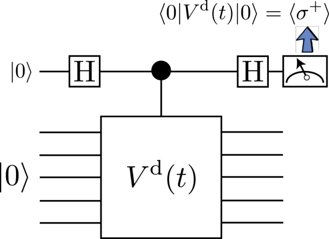
We can combine Thms. 1 and 2 to construct a quantum algorithm to simulate the QHO and obtain the desired propagators ⟨φ′|U⁡(t)|φ⟩\langle\varphi^{\prime}|U(t)|\varphi\rangle. The quantum algorithm has three basic steps: i- the preparation of an initial state, ii- the implementation or simulation of the evolution operator, and iii- a projective measurement. The desired expectation value can be obtained within arbitrary accuracy after repeated executions of these steps. The simulation of the evolution operator induced by HdH^{\rm d} was discussed in Sec. IV.1. We let WφdW^{\rm d}_{\varphi} and Wφ′dW^{\rm d}_{\varphi^{\prime}} be the N×NN\times N unitary matrices that prepare the states |φd⟩|\varphi^{\rm d}\rangle and |φ′d⟩|\varphi^{\prime{\rm d}}\rangle, from e.g. |0⟩|0\rangle, respectively. We also let Vd​(t)=(Wφ′d)†​Ud​(t)​WφdV^{\rm d}(t)=(W^{\rm d}_{\varphi^{\prime}})^{\dagger}U^{\rm d}(t)W^{\rm d}_{\varphi}, so the propagator of interest is ⟨0|Vd​(t)|0⟩\langle 0|V^{\rm d}(t)|0\rangle. To measure such expectation values at precision ϵ\epsilon, we can implement the quantum circuit in Fig. 6, O⁡(1/ϵ)O(1/\sqrt{\epsilon}) times [40, 5]. Otherwise, we can implement the quantum methods described in [31] for optimal quantum measurements of overlaps, where the number of repetitions can be improved to O⁡(1/ϵ)O(1/\epsilon).

Refer to caption
Figure 6: Quantum circuit to compute the propagator ⟨0|Vd​(t)|0⟩\langle 0|V^{\rm d}(t)|0\rangle, where Vd​(t)V^{\rm d}(t) is unitary [40, 5]. The filled circle denotes the controlled operation on the state |1⟩|1\rangle of the ancilla qubit; that is, the corresponding unitary operation is 1​l⊗|0⟩​⟨0|+Vd​(t)⊗|1⟩​⟨1|{\mathchoice{\rm 1\mskip-4.0mul}{\rm 1\mskip-4.0mul}{\rm 1\mskip-4.5mul}{\rm 1\mskip-5.0mul}}\otimes|0\rangle\langle 0|+V^{\rm d}(t)\otimes|1\rangle\langle 1|. H denotes the Hadamard gate that maps the state of a qubit as H|0⟩=(|0⟩+|1⟩)/2{\rm H}\left|0\right\rangle=(\left|0\right\rangle+\left|1\right\rangle)/\sqrt{2} and H|1⟩=(|0⟩−|1⟩)/2{\rm H}\left|1\right\rangle=(\left|0\right\rangle-\left|1\right\rangle)/\sqrt{2}. The single qubit operator σ+\sigma^{+} is σx+i​σy\sigma_{x}+i\sigma_{y}, with σα\sigma_{\alpha} the Pauli operators. Since σ+\sigma^{+} is not Hermitian, the computation of its expectation value can be done by repeated projective measurements of σx\sigma_{x} and σy\sigma_{y} independently (i.e., with repeated executions of the circuit).

In the rest of this section we assume that the precision ϵ≪1\epsilon\ll 1 is constant, i.e., ϵ=O⁡(1)\epsilon=O(1). We also assume that WφdW^{\rm d}_{\varphi} and Wφ′dW^{\rm d}_{\varphi^{\prime}} can be efficiently implemented using O⁡(polylog⁡(N))O({\rm polylog}(N)) gates. Then, Thms. 1 and 2 imply

Theorem 3.

Let |φ⟩=∑n=0N′cn​|ψn⟩|\varphi\rangle=\sum_{n=0}^{N^{\prime}}c_{n}|\psi_{n}\rangle, |φ′⟩=∑n=0N′cn′​|ψn⟩|\varphi^{\prime}\rangle=\sum_{n=0}^{N^{\prime}}c^{\prime}_{n}|\psi_{n}\rangle or |φ′⟩=(2​π/N)1/4​|xj⟩|\varphi^{\prime}\rangle=(2\pi/N)^{1/4}|x_{j}\rangle and tt the evolution time. Assume |t|≥1|t|\geq 1 and, with no loss of generality, t=O⁡(1)t=O(1). Then, there exists a quantum algorithm 𝒬\cal Q that outputs ⟨φ′|U⁡(t)|φ⟩\langle\varphi^{\prime}|U(t)|\varphi\rangle at arbitrary accuracy. 𝒬\cal Q requires ℳ𝒬=O⁡(exp⁡(γ′​log⁡(N′))){\cal M}_{\cal Q}=O(\exp(\gamma^{\prime}\sqrt{\log(N^{\prime})})) two-qubit gates, where γ′>0\gamma^{\prime}>0 is a constant.

Proof.

Let N=exp⁡(O⁡(log⁡(N′​|t|)))+O⁡(N′)N=\exp(O(\sqrt{\log(N^{\prime}|t|)}))+O(N^{\prime}), p=O⁡(log⁡(N′​|t|))p=O(\sqrt{\log(N^{\prime}|t|)}), and |s|=exp⁡(−O⁡(log⁡(N′​|t|)))|s|=\exp(-O(\sqrt{\log(N^{\prime}|t|)})) as in Lemma 8 or the proof of Thm. 2, for ϵ=O⁡(1)\epsilon=O(1). The subadditivity property of errors implies (k=t/sk=t/s)

⟨φ′|U⁡(t)|φ⟩\displaystyle\langle\varphi^{\prime}|U(t)|\varphi\rangle =⟨φ′d|(Upd​(s))k|φd⟩+O⁡(ϵ)\displaystyle=\langle\varphi^{\prime{\rm d}}|(U^{\rm d}_{p}(s))^{k}|\varphi^{\rm d}\rangle+O(\epsilon)
=⟨0|(Wφ′d)†​(Upd​(s))k​Wφd|0⟩+O⁡(ϵ),\displaystyle=\langle 0|(W_{\varphi^{\prime}}^{\rm d})^{\dagger}(U^{\rm d}_{p}(s))^{k}{W_{\varphi}^{\rm d}}|0\rangle+O(\epsilon)\;, (32)

with ϵ≪1\epsilon\ll 1. Then, we can use the circuit of Fig. 6, a constant number of times, with a unitary Vd​(t)=(Wφ′d)†​(Upd​(s))k​WφdV^{\rm d}(t)=(W_{\varphi^{\prime}}^{\rm d})^{\dagger}(U^{\rm d}_{p}(s))^{k}{W_{\varphi}^{\rm d}} to output the desired propagator. Since Wφ′dW_{\varphi^{\prime}}^{\rm d} and WφdW_{\varphi}^{\rm d} can be efficiently implemented, the complexity of the quantum algorithm is dominated by the number of two-qubit gates needed to implement (Upd​(s))k(U^{\rm d}_{p}(s))^{k} within the desired accuracy. Theorem 2 implies that such a number is O⁡(|t|​exp⁡(γ′​log⁡(N′​|t|)))O(|t|\exp(\gamma^{\prime}\sqrt{\log(N^{\prime}|t|)})), for some constant γ′>0\gamma^{\prime}>0. The result follows by assuming, with no loss of generality, t=O⁡(1)t=O(1). ∎

It is important to remark that the complexity of the quantum algorithm satisfies

limN′→∞ℳ𝒬/N′η=0,\displaystyle\lim_{N^{\prime}\rightarrow\infty}{\cal M}_{\cal Q}/N^{\prime\eta}=0\;, (33)

for all η>0\eta>0, and limN′→∞log⁡(N′)/ℳ𝒬=0\lim_{N^{\prime}\rightarrow\infty}\log(N^{\prime})/{\cal M}_{\cal Q}=0. That is, the complexity of the quantum algorithm is subexponential in log⁡(N′)\log(N^{\prime}). Since classical algorithms are expected to require poly⁡(N′){\rm poly}(N^{\prime}) operations to compute the propagator in the worst case, our quantum algorithm provides a superpolynomial quantum speedup.

V Eigenstate preparation

We now investigate ways of simulating and preparing low-energy eigenstates of HdH^{\rm d}, via the action of unitary operations acting on simple initial states. In part, this section addresses the second goal of a QS, namely the computation of expectation values on various eigenstates of the QHO, which can be obtained using the techniques presented in previous sections if we replace the initial state |φ⟩|\varphi\rangle by the corresponding |ψn⟩|\psi_{n}\rangle (or |φd⟩|\varphi^{\rm d}\rangle by |ϕnd⟩|\phi_{n}^{\rm d}\rangle). The results of this section may be of independent interest; e.g., quantum algorithms to prepare states with Gaussian-like amplitudes are important in other cases [41].

We first focus on the preparation of the ground state |ϕ0d⟩|\phi_{0}^{\rm d}\rangle. In Appx. C, Lemma 9, we prove in the large-NN limit,

‖|ψ0d⟩−e−i​α​(t)​ei​(xd)2​t′​ei​(pd)2​t​|φd⟩‖=O⁡(exp⁡(−Ω⁡(δ))),\displaystyle\||\psi_{0}^{\rm d}\rangle-e^{-i\alpha(t)}e^{i(x^{\rm d})^{2}t^{\prime}}e^{i(p^{\rm d})^{2}t}|\varphi^{\rm d}\rangle\|=O(\exp(-\Omega(\delta)))\;, (34)

where the initial state is

(1/κ)∑j=−N/2N/2exp(−j2/(2δ))|j⟩,\displaystyle(1/\sqrt{\kappa})\sum_{j=-N/2}^{N/2}\exp(-j^{2}/(2\delta))\left|j\right\rangle\;, (35)

and δ>0\delta>0. The constant κ\kappa is for normalization purporses and α⁡(t)\alpha(t) is an irrelevant global phase that can be computed exactly. The evolution times satisfy t=σ2​(2−4​σ2)/2t=\sqrt{\sigma^{2}(2-4\sigma^{2})}/2 and t′=1/(4​t+4​σ2/t)t^{\prime}=1/(4t+4\sigma^{2}/t), and σ2=π​δ/N\sigma^{2}=\pi\delta/N. This result was obtained by realizing that in CVs, the quantum state |ψ0⟩|\psi_{0}\rangle can be obtained from an initial state with Gaussian-like amplitudes by evolving with the free-particle Hamiltonian (i.e., −p^2-\hat{p}^{2}). The result follows by approximating the CV case after a proper discretization.

Lemma 9 allows us to state the first result of this section.

Theorem 4.

Let ϵ>0\epsilon>0. Then, there is a unitary WdW^{\rm d} that satisfies

∥|ϕ0d⟩−Wd|0⟩∥=O(ϵ)\displaystyle\||\phi_{0}^{\rm d}\rangle-W^{\rm d}\left|0\right\rangle\|=O(\epsilon) (36)

in the large NN limit. WdW^{\rm d} can be implemented on a quantum computer using a number of two-qubit gates that is polynomial in log⁡(N/ϵ)\log(N/\epsilon).

Proof.

First, we choose δ=O⁡(log⁡(1/ϵ))\delta=O(\log(1/\epsilon)) so that the right hand side of Eq. (34) is O⁡(ϵ)O(\epsilon). In the large NN limit, |ψ0d⟩|\psi_{0}^{\rm d}\rangle can be safely replaced by |ϕ0d⟩|\phi_{0}^{\rm d}\rangle in Eq. (34), as the error of this replacement is exponentially small in NN and thus negligible. Next, we note that we can approximate |φd⟩|\varphi^{\rm d}\rangle within error O⁡(ϵ)O(\epsilon) by

∝∑j=−j0j0e−j2/(2δ)|j⟩,\displaystyle\propto\sum_{j=-j_{0}}^{j_{0}}e^{-j^{2}/(2\delta)}\left|j\right\rangle\;, (37)

with j0=O⁡(log⁡(1/ϵ)​δ)=O⁡(log⁡(1/ϵ))j_{0}=O(\sqrt{\log(1/\epsilon)\delta})=O(\log(1/\epsilon)). The state of Eq. (37) can be prepared with complexity polynomial in log⁡(1/ϵ)\log(1/\epsilon) using standard techniques. We write VdV^{\rm d} for the unitary that prepares such a state and define Wd=e−i​α​(t)​ei​(xd)2​t′​ei​(pd)2​t​VdW^{\rm d}=e^{-i\alpha(t)}e^{i(x^{\rm d})^{2}t^{\prime}}e^{i(p^{\rm d})^{2}t}V^{\rm d}, with the choices of tt and t′t^{\prime} given above. Because t=O⁡(1/N)t=O(1/\sqrt{N}) and t′=O⁡(N)t^{\prime}=O(\sqrt{N}) in the large NN limit, the unitaries ei​(xd)2​t′e^{i(x^{\rm d})^{2}t^{\prime}} and ei​(pd)2​te^{i(p^{\rm d})^{2}t} can be implemented on a quantum computer with complexity polynomial in log⁡(1/ϵ)\log(1/\epsilon) and log⁡(N)\log(N) [i.e., polynomial in log⁡(N/ϵ)\log(N/\epsilon)] – see Sec. IV.1. ∎

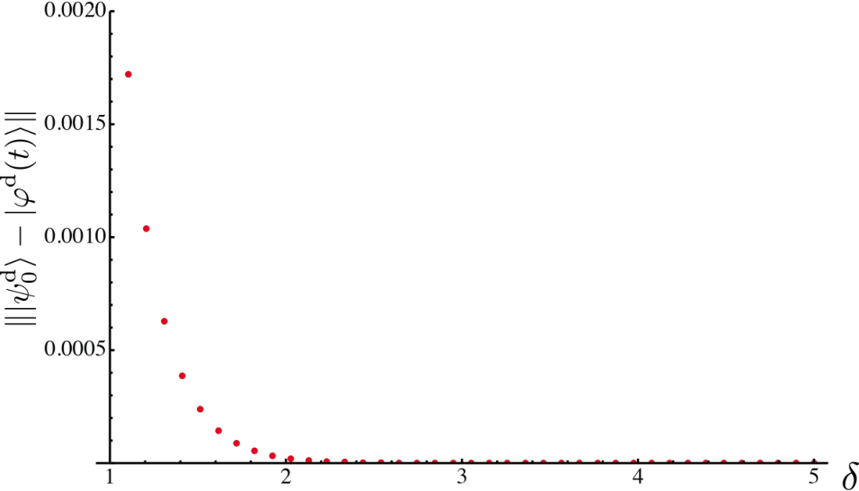
In Fig. 7 we show the exponential decay of the error as a function of δ\delta, as stated by the theorem. We note that quantum methods to prepare states with Gaussian-like amplitudes were also proposed in [41, 42].
Refer to caption
Figure 7: The norm of the difference between the state |ψ0d⟩|\psi_{0}^{\rm d}\rangle and the evolved state |φd​(t)⟩=e−i​α​(t)​ei​(xd)2​t′​e−i​(pd)2​t​|φd⟩|\varphi^{\rm d}(t)\rangle=e^{-i\alpha(t)}e^{i(x^{\rm d})^{2}t^{\prime}}e^{-i(p^{\rm d})^{2}t}|\varphi^{\rm d}\rangle, as a function of δ\delta and for N=800N=800. Numerical simulations do not show significant changes for larger dimensions.

To prepare the other eigenstates |ϕnd⟩|\phi_{n}^{\rm d}\rangle, with n≥1n\geq 1, we define a discrete version of the Jaynes-Cummings (JC) model:

HJCd=(xd⊗σx−pd⊗σy)/2,\displaystyle H^{\rm d}_{\rm JC}=(x^{\rm d}\otimes\sigma_{x}-p^{\rm d}\otimes\sigma_{y})/\sqrt{2}\;, (38)

where σα\sigma_{\alpha} are the corresponding Pauli operators acting on a the Hilbert space of an ancillary qubit. In CV, the evolution induced by the JC model eventually transforms the state |ψn⟩|0⟩|\psi_{n}\rangle\left|0\right\rangle into |ψn+1⟩|1⟩|\psi_{n+1}\rangle\left|1\right\rangle, providing a unitary operation to prepare eigenstates of the QHO from |ψ0⟩|\psi_{0}\rangle. We will show that something similar occurs in the discrete case.

For n≥0n\geq 0, we define the normalized states

|γn,±d⟩=12[|ϕnd⟩|0⟩±|ϕn+1d⟩|1⟩].\displaystyle|\gamma^{\rm d}_{n,\pm}\rangle=\frac{1}{\sqrt{2}}[|\phi_{n}^{\rm d}\rangle\left|0\right\rangle\pm|\phi_{n+1}^{\rm d}\rangle\left|1\right\rangle]\;. (39)

These are approximations of the eigenstates of HJCdH^{\rm d}_{\rm JC}. In Appx. D, Lemma 10, we show that if n≤N′≤c​Nn\leq N^{\prime}\leq cN, for some constant c>0c>0,

‖(HJCd∓n+1)​|γn,±d⟩‖=ν1​(N).\displaystyle\|(H^{\rm d}_{\rm JC}\mp\sqrt{n+1})|\gamma^{\rm d}_{n,\pm}\rangle\|=\nu_{1}(N)\;. (40)

We use Eq. (40) to prove the second result of this section.

Theorem 5.

Let ϵ>0\epsilon>0 and tn=π/(2​n+1)t_{n}=\pi/(2\sqrt{n+1}). Then, there exists N=O⁡(log⁡(1/ϵ)+N′)N=O(\log(1/\epsilon)+N^{\prime}) such that

∥e−i​HJCd​tn|ϕnd⟩|0⟩+i|ϕn+1d⟩|1⟩∥=O(ϵ),\displaystyle\|e^{-iH_{\rm JC}^{\rm d}{t_{n}}}|\phi_{n}^{\rm d}\rangle\left|0\right\rangle+i|\phi_{n+1}^{\rm d}\rangle\left|1\right\rangle\|=O(\epsilon)\;, (41)

for all n≤N′n\leq N^{\prime}.

Proof.

We let N≥N′/cN\geq N^{\prime}/c. Then, Eq. (40) implies

‖[e−i​HJCd​tn−e−i⁡(±n+1​tn)]​|γn,±d⟩‖=|tn|​ν1​(N),\displaystyle\|[e^{-iH_{\rm JC}^{\rm d}{t_{n}}}-e^{-i(\pm\sqrt{n+1}t_{n})}]|\gamma^{\rm d}_{n,\pm}\rangle\|=|t_{n}|\nu_{1}(N)\;, (42)

for all n≤N′n\leq N^{\prime}. For tn=π/(2​n+1)t_{n}=\pi/(2\sqrt{n+1}), this implies ‖(e−i​HJCd​tn±i)​|γn,±d⟩‖=ν1​(N)\|(e^{-iH_{\rm JC}^{\rm d}t_{n}}\pm i)|\gamma^{\rm d}_{n,\pm}\rangle\|=\nu_{1}(N), and then

∥e−i​HJCd​tn|ϕnd⟩|0⟩+i|ϕn+1d⟩|1⟩∥=ν1(N).\displaystyle\|e^{-iH_{\rm JC}^{\rm d}t_{n}}|\phi_{n}^{\rm d}\rangle\left|0\right\rangle+i|\phi_{n+1}^{\rm d}\rangle\left|1\right\rangle\|=\nu_{1}(N)\;. (43)

Then, there is N=O⁡(log⁡(1/ϵ))N=O(\log(1/\epsilon)) so that the right hand side of Eq. (43) is O⁡(ϵ)O(\epsilon). ∎

We can combine Thms. 4 and 5 to prepare approximations of other eigenstates |ϕnd⟩|\phi_{n}^{\rm d}\rangle, n≥1n\geq 1, by a sequential action of (1​l⊗σx).e−i​HJCd​tn({\mathchoice{\rm 1\mskip-4.0mul}{\rm 1\mskip-4.0mul}{\rm 1\mskip-4.5mul}{\rm 1\mskip-5.0mul}}\otimes\sigma_{x}).e^{-iH_{\rm JC}^{\rm d}t_{n}} on the initial state |ϕ0d⟩|0⟩|\phi_{0}^{\rm d}\rangle\left|0\right\rangle. The Pauli operator σx\sigma_{x} is necessary to transform |1⟩→|0⟩\left|1\right\rangle\rightarrow\left|0\right\rangle for the state of the ancilla qubit at each step. Then,

|ϕnd⟩|0⟩≈∏n′=0n−1(1l⊗σx)e−i​HJCd​tn′|ϕ0d⟩|0⟩.\displaystyle|\phi_{n}^{\rm d}\rangle\left|0\right\rangle\approx\prod_{n^{\prime}=0}^{n-1}({\mathchoice{\rm 1\mskip-4.0mul}{\rm 1\mskip-4.0mul}{\rm 1\mskip-4.5mul}{\rm 1\mskip-5.0mul}}\otimes\sigma_{x})e^{-iH_{\rm JC}^{\rm d}t_{n^{\prime}}}|\phi_{0}^{\rm d}\rangle\left|0\right\rangle\;. (44)

We now seek a quantum algorithm to prepare the eigenstates |ϕnd⟩|\phi_{n}^{\rm d}\rangle, up to a given approximation error. This requires giving a quantum circuit to approximate each e−i​HJCd​tn′e^{-iH_{\rm JC}^{\rm d}t_{n^{\prime}}} in Eq. (44). Since the unitaries e−i⁡(xd⊗σx)​te^{-i(x^{\rm d}\otimes\sigma_{x})t} and e−i⁡(pd⊗σy)​te^{-i(p^{\rm d}\otimes\sigma_{y})t} can be simulated within precision ϵ~\tilde{\epsilon} using a number of two-qubit gates that is polylog⁡(N​|t|/ϵ~){\rm polylog}(N|t|/\tilde{\epsilon}) (Sec. IV.1), we will use the Trotter-Suzuki approximation. In Appx. D, Lemma 11, we show that if s=O⁡(ϵ/n+1)s=O(\epsilon/\sqrt{n+1}) for some n≤N′≤c​Nn\leq N^{\prime}\leq cN, then

∥[e−i(xd⊗σx)s/2ei⁡(pd⊗σy)​s/2−e−i​HJCd​s]|γn,±d⟩∥=O(ϵ2).\displaystyle\|[e^{-i(x^{\rm d}\otimes\sigma_{x})s/\sqrt{2}}e^{i(p^{\rm d}\otimes\sigma_{y})s/\sqrt{2}}-e^{-iH_{\rm JC}^{\rm d}s}]|\gamma^{\rm d}_{n,\pm}\rangle\|=O(\epsilon^{2})\;. (45)

The proof uses a simple Trotter-Suzuki approximation and the scaling with ϵ\epsilon can be improved using higher order approximations. We can use this result to prove:

Theorem 6.

Let ϵ>0\epsilon>0. Then, there is a quantum circuit WdW^{\rm d} that satisfies

∥Wd|ϕ0d⟩|0⟩−|ϕnd⟩|0⟩∥=O(ϵ)\displaystyle\|W^{\rm d}|\phi_{0}^{\rm d}\rangle\left|0\right\rangle-|\phi_{n}^{\rm d}\rangle\left|0\right\rangle\|=O(\epsilon)\; (46)

for any given n≤N′≤c​Nn\leq N^{\prime}\leq cN, where NN is the dimension of the Hilbert space and c>0c>0 is a constant. WdW^{\rm d} can be implemented using a number of two-qubit gates that is O⁡((n2/ϵ)​polylog​(N/ϵ))O((n^{2}/\epsilon){\rm polylog}(N/\epsilon)).

Proof.

The quantum circuit is

Wd=∏n′=0n−1(1l⊗σx)[e−i(xd⊗σx)tn′/(m2)ei⁡(pd⊗σy)​tn′/(m​2)]m.\displaystyle W^{\rm d}=\prod_{n^{\prime}=0}^{n-1}({\mathchoice{\rm 1\mskip-4.0mul}{\rm 1\mskip-4.0mul}{\rm 1\mskip-4.5mul}{\rm 1\mskip-5.0mul}}\otimes\sigma_{x})\left[e^{-i(x^{\rm d}\otimes\sigma_{x})t_{n^{\prime}}/(m\sqrt{2})}e^{i(p^{\rm d}\otimes\sigma_{y})t_{n^{\prime}}/(m\sqrt{2})}\right]^{m}. (47)

Here, m=O⁡(n/ϵ)m=O(n/\epsilon) so that each term in WdW^{\rm d} introduces an error O⁡(ϵ/n)O(\epsilon/n) as implied by Lemma 11. Because we work in the asymptotic limit, approximation errors that are exponentially small in NN or N\sqrt{N} are negligible. Then,

∥Wd|ϕ0d⟩|0⟩−|ϕnd⟩|0⟩∥=O((ϵ/n)n)=O(ϵ).\displaystyle\|W^{\rm d}|\phi_{0}^{\rm d}\rangle\left|0\right\rangle-|\phi_{n}^{\rm d}\rangle\left|0\right\rangle\|=O((\epsilon/n)n)=O(\epsilon)\;. (48)

The number of terms in the product is O⁡(n2/ϵ)O(n^{2}/\epsilon). The number of two-qubit gates is then

O⁡((n2/ϵ)​polylog​(N/ϵ)).\displaystyle O((n^{2}/\epsilon){\rm polylog}(N/\epsilon))\;. (49)

∎

VI The quartic potential

We now analyze quantum algorithms to simulate the evolution operator of a quantum system with Hamiltonian H=12​(p^2+x^4)H=\frac{1}{2}(\hat{p}^{2}+\hat{x}^{4}). We will use the same discretization as that for the DQHO, where xdx^{\rm d} and pdp^{\rm d} where defined in Sec. III. Then,

Hd=12​((pd)2+(xd)4).\displaystyle H^{\rm d}=\frac{1}{2}((p^{\rm d})^{2}+(x^{\rm d})^{4})\;. (50)

In contrast to previous sections, we only conduct a numerical analysis here and state some observations from numerical results. In part, this is due to not having an exact solution in this case. Our simulations suggest a polynomial speedup for the computation of scattering amplitudes.

In Fig. 8 we plot the eigenvalues End​(N)E_{n}^{\rm d}(N) of HdH^{\rm d} for different dimensions NN and as a function of n=0,1,…,N−1n=0,1,\ldots,N-1. Taking dimension 40004000 as a reference, in Table 1 we look for the maximum value of nn such that |End​(N)−End​(4000)||E_{n}^{\rm d}(N)-E_{n}^{\rm d}(4000)| is below some threshold ϵi≪1\epsilon^{i}\ll 1. The values of the ratios rir^{i} suggest that the eigenvalues of a large sector of the low-energy subspace of the CV system can be well approximated by those of the discrete system. While rir^{i} does seem to decrease in NN, the scaling does not seem to be of the form 1/Nχ1/N^{\chi}, for some χ>0\chi>0, but rather of the form 1/log⁡N1/\log N. If this is the case, then, to approximate up to the nn-th eigenvalue of HH, it suffices to choose N=O⁡(n​log⁡n)N=O(n\log n) for the discrete system. Nevertheless, both the classical and quantum algorithms to simulate this system will have complexity that depend on the same value of NN, and the dependence of rir^{i} on NN is unimportant to demonstrate a quantum speedup.

Refer to caption
Figure 8: Eigenvalues of HdH^{\rm d} for N=4000N=4000 (blue), N=3200N=3200 (yellow), and N=1600N=1600 (purple).
NN n1n^{1} r1r^{1} n2n^{2} r2r^{2}
100 16 0.16 12 0.12
200 30 0.15 27 0.135
400 57 0.1425 54 0.135
800 105 0.1312 99 0.125
1600 181 0.1131 177 0.1106
2000 216 0.108 212 0.106
3200 314 0.0981 310 0.0968
Table 1: nin^{i}, maximum value of nn such that |End​(N)−End​(4000)|≤ϵi|E_{n}^{\rm d}(N)-E_{n}^{\rm d}(4000)|\leq\epsilon^{i}, for ϵ1=10−5\epsilon^{1}=10^{-5} and ϵ2=10−7\epsilon^{2}=10^{-7}. The ratios are ri=ni/Nr^{i}=n^{i}/N.

We can use the Trotter-Suzuki approximation to simulate the evolution operator Ud​(t)=exp⁡{−i​Hd​t}U^{\rm d}(t)=\exp\{-iH^{\rm d}t\}. This approximation splits the evolution operator into a product of exponentials or short time evolutions under (pd)2(p^{\rm d})^{2} and (xd)4(x^{\rm d})^{4} and, using the result of Sec. IV.1, each of these exponentials can be simulated efficiently. In contrast to the QHO, the operators x^4\hat{x}^{4} and p^2\hat{p}^{2} do not form a small dimensional Lie algebra and tight error bounds from high-order Trotter-Suzuki approximations may be difficult to obtain. The recursive definition for Upd​(s)U_{p}^{\rm d}(s) is given in Eq. (29), assuming

U1d(s):=e−is(xd)4/4e−is(pd)2/2e−is(xd)4/4.\displaystyle U_{1}^{\rm d}(s):=e^{-is(x^{\rm d})^{4}/4}e^{-is(p^{\rm d})^{2}/2}e^{-is(x^{\rm d})^{4}/4}\;. (51)

A worst-case analysis of the Trotter-Suzuki formula results in an approximation error bounded by ϵp​(s)=O⁡(|s|2​p+1​‖Hd‖2​p+1)=O⁡((|s|​N2)2​p+1)\epsilon_{p}(s)=O(|s|^{2p+1}\|H^{\rm d}\|^{2p+1})=O((|s|N^{2})^{2p+1}) [19, 38, 14, 39, 15, 18]. However, as in the case of the DQHO, we would expect that the error for the current case is significantly smaller than that for the worst case. This is because the operators in HH, while they do not form a finite dimensional Lie algebra, posses an algebraic structure that results in an effective norm for nested commutators that is significantly smaller than the product of the effective norms [32]. In Fig. 9 we plot the error ‖(Upd​(s)−Ud​(s))​|ϕnd⟩‖\|(U_{p}^{\rm d}(s)-U^{\rm d}(s))|\phi_{n}^{\rm d}\rangle\| as a function of nn, for |s|=O⁡(1)|s|=O(1), and p=1,2,3p=1,2,3. Here, |ϕnd⟩|\phi_{n}^{\rm d}\rangle are the eigenstates of HdH^{\rm d} in Eq. (50) and cannot be approximated by the discrete Hermite states |ψnd⟩|\psi_{n}^{\rm d}\rangle. The results suggest ∥(Upd(s)−Ud(s))|ϕnd⟩∥=O(|s|2​p+1n(2​p+4)/3)\|(U_{p}^{\rm d}(s)-U^{\rm d}(s))\left|\phi_{n}^{\rm d}\right\rangle\|=O(|s|^{2p+1}n^{(2p+4)/3}). The order dependence in ss follows from the analysis of the high-order Trotter-Suzuki approximations and was verified by additional numerical simulations, to assure that we are in a region of convergence.

Refer to caption
Figure 9: The error from high-order Trotter-Suzuki approximations (red dots) as a function of nn. The results are for dimension N=1600N=1600, s=0.01s=0.01, and for n=0,1,…,181n=0,1,...,181, according to Table 1. Our simulations suggest that the error is O⁡(s2​p+1​np′)O(s^{2p+1}n^{p^{\prime}}), where p′p^{\prime} depends on pp. (a) p=1p=1. The blue line indicates a fit with the function f1=3.44.10−7​n2f_{1}=3.44.10^{-7}\;n^{2}. (b) p=2p=2. The blue line indicates a fit with the function f1=7.8.10−12​n8/3f_{1}=7.8.10^{-12}n^{8/3}. (c) p=3p=3. The blue line indicates a fit with the function f3=3.3.10−17​n10/3f_{3}=3.3.10^{-17}\;n^{10/3}.

Under these numerical observations, we can analyze the complexity of a quantum algorithm that computes scattering amplitudes

⟨φ′|U(t)|φ⟩,\displaystyle\left\langle\varphi^{\prime}\right|U(t)\left|\varphi\right\rangle\;, (52)

within some precision ϵ\epsilon. For simplicity, we assume that the initial and final states, |φ⟩|\varphi\rangle and |φ′⟩|\varphi^{\prime}\rangle, can be written as linear superpositions of the eigenstates |ϕn⟩|\phi_{n}\rangle, with n≤N′n\leq N^{\prime}. This suggests that we can approximate Eq. (52) by ⟨φ′d|Ud​(t)|φd⟩\langle\varphi^{\prime{\rm d}}|U^{\rm d}(t)|\varphi^{\rm d}\rangle , where the dimension is N=O⁡(N′​log⁡(N′))N=O(N^{\prime}\log(N^{\prime})), and |φd⟩|\varphi^{\rm d}\rangle and |φ′d⟩|\varphi^{\prime{\rm d}}\rangle are quantum states obtained by replacing |ϕn⟩|\phi_{n}\rangle by |ϕnd⟩|\phi_{n}^{\rm d}\rangle in the spectral decompositions of |φ⟩|\varphi\rangle and |φ′⟩|\varphi^{\prime}\rangle, respectively. We assume that |φd⟩|\varphi^{\rm d}\rangle and |φ′d⟩|\varphi^{\prime{\rm d}}\rangle can be efficiently prepared so that the main cost of the algorithm is that from simulating Ud​(t)U^{\rm d}(t). We split the evolution time into kk parts of size s=t/ks=t/k. Using the (2​p+1)(2p+1)-th order Trotter-Suzuki approximation, our numerical simulations suggest that the error is bounded by k​ω​(ω′​|s|)2​p+1​N(2​p+4)/3k\omega(\omega^{\prime}\;|s|)^{2p+1}N^{(2p+4)/3}. ω\omega and ω′>1\omega^{\prime}>1 are constants. Replacing ss by t/kt/k, the number of terms in the product formula is

k​5p=O⁡(|t|1+1/2​p​N(1+2/p)/3ϵ1/2​p​5p).\displaystyle k5^{p}=O\left(\frac{|t|^{1+1/2p}N^{(1+2/p)/3}}{\epsilon^{1/2p}}5^{p}\right)\;. (53)

As pp grows large, the number of terms can be made O⁡(|t|1+η​N1/3+4​η/3/ϵη)O(|t|^{1+\eta}N^{1/3+4\eta/3}/\epsilon^{\eta}), for arbitrary small η\eta. Then, the quantum circuit that approximates the evolution operator Ud​(t)U^{\rm d}(t), needed to compute Eq. (52), can be implemented using a number of two-qubit gates that is

ℳ𝒬=O⁡(|t|1+η​N1/3+4​η/3ϵη​polylog​(N​t/ϵ)).\displaystyle{\cal M_{Q}}=O\left(\frac{|t|^{1+\eta}N^{1/3+4\eta/3}}{\epsilon^{\eta}}{\rm polylog}(Nt/\epsilon)\right)\;. (54)

This complexity represents a polynomial quantum speedup, with respect to NN, over the quantum algorithm that approximates scattering amplitudes for the quartic potential. Classical algorithms, in the worst-case, may require computing and obtaining the spectral properties of Ud​(t)U^{\rm d}(t), which can be done in complexity O⁡(Nσ)O(N^{\sigma}), for σ>2\sigma>2.

VII One-dimensional quantum systems: An upper bound

We now present an upper bound on the complexity of simulating the evolution operator of one-dimensional quantum systems described by H=12​p^2+V⁡(x^)H=\frac{1}{2}\hat{p}^{2}+V(\hat{x}), where V⁡(x^)V(\hat{x}) is the potential, i.e., some operator that depends on x^\hat{x}. If |ϕn⟩\left|\phi_{n}\right\rangle, n=0,1,…n=0,1,\ldots, denote the eigenstates of HH and |φ⟩\left|\varphi\right\rangle is the initial state, we will assume |φ⟩=∑n=0N′cn|ϕn⟩\left|\varphi\right\rangle=\sum_{n=0}^{N^{\prime}}c_{n}\left|\phi_{n}\right\rangle and ∥V(x^)|ϕn⟩∥=O(poly(N′))\|V(\hat{x})\left|\phi_{n}\right\rangle\|=O({\rm poly}(N^{\prime})), for all n≤N′n\leq N^{\prime}.

We also assume that there exists N<∞N<\infty, the dimension of the Hilbert space, such that, if

Hd=12​(pd)2+V⁡(xd),\displaystyle H^{\rm d}=\frac{1}{2}(p^{\rm d})^{2}+V(x^{\rm d})\;, (55)

the scattering amplitudes of the CV system can be well approximated by those of the discrete system. NN will depend on N′N^{\prime} and the precision parameter ϵ\epsilon. In particular, for constant precision, we will assume that N=O⁡(poly⁡(N′))N=O({\rm poly}(N^{\prime})), an assumption that is satisfied by a large class of one-dimensional quantum systems such as the QHO or the quartic potential.

Theorem 7.

Let ϵ>0\epsilon>0 and tt be the evolution time, |t|=Ω⁡(1)|t|=\Omega(1). Then, there is a quantum circuit WdW^{\rm d} that satisfies

∥(Wd−Ud(t))|φd⟩∥≤ϵ,\displaystyle\|(W^{\rm d}-U^{\rm d}(t))\left|\varphi^{\rm d}\right\rangle\|\leq\epsilon\;, (56)

for all |φd⟩∝∑n=0N′cn|ϕnd⟩\left|\varphi^{\rm d}\right\rangle\propto\sum_{n=0}^{N^{\prime}}c_{n}|\phi^{\rm d}_{n}\rangle. Here, |ϕnd⟩|\phi^{\rm d}_{n}\rangle are the eigenstates of HdH^{\rm d} and Ud​(t)=exp⁡{−i​Hd​t}U^{\rm d}(t)=\exp\{-iH^{\rm d}t\}. WdW^{\rm d} can be implemented using O⁡(N​|t|​polylog​(N​|t|/ϵ))O(N|t|{\rm polylog}(N|t|/\epsilon)) two-qubit gates.

Proof.

We use our results in [21] for Hamiltonian simulation and do some modifications to obtain the desired result. In [21] we showed that for a dd-sparse time dependent Hamiltonian A⁡(t)A(t) acting on qq qubits, the evolution operator can be approximated within precision ϵ\epsilon using

O⁡(q​d2​‖A‖max​|t|​log⁡((d2​‖A‖max+‖A˙‖)​|t|/ϵ)log⁡log⁡(d2​‖A‖max​|t|/ϵ)CLOSE\displaystyle O(qd^{2}\|A\|_{\max}|t|\frac{\log((d^{2}\|A\|_{\max}+\|\dot{A}\|)|t|/\epsilon)}{\log\log(d^{2}\|A\|_{\max}|t|/\epsilon)} (57)

two-qubit gates, where A˙=∂tA\dot{A}=\partial_{t}A and the norms are the maximum norms in the time interval [0,t][0,t]. The gate cost results from a decomposition of A⁡(t)A(t) in terms of O⁡(d2​‖A‖max)O(d^{2}\|A\|_{\max}) unitary operators. Since HdH^{\rm d} is not sparse and its norm can be larger than O⁡(N)O(N), Eq. (57) would result in a large gate complexity in this case. To overcome this difficulty, we analyze the evolution operator in the interaction picture. We then define the time-dependent interaction Hamiltonian

HId​(s)\displaystyle H^{\rm d}_{I}(s) =12​ei​V​(xd)​s​(pd)2​e−i​V​(xd)​s\displaystyle=\frac{1}{2}e^{iV(x^{\rm d})s}(p^{\rm d})^{2}e^{-iV(x^{\rm d})s}
=12​ei​V​(xd)​s​(Fcd)−1​(xd)2​Fcd​e−i​V​(xd)​s,\displaystyle=\frac{1}{2}e^{iV(x^{\rm d})s}(F_{\rm c}^{\rm d})^{-1}(x^{\rm d})^{2}F_{\rm c}^{\rm d}e^{-iV(x^{\rm d})s}\;, (58)

and denote UId​(t)U^{\rm d}_{I}(t) for the corresponding evolution. Since xdx^{\rm d} is 1-sparse and ‖xd‖=O⁡(N)\|x^{\rm d}\|=O(\sqrt{N}), we obtain ‖HId‖max=O⁡(N)\|H^{\rm d}_{I}\|_{\max}=O(N) and HId​(s)H^{\rm d}_{I}(s) can be decomposed as a sum of O⁡(N)O(N) unitary operators. In addition, ‖H˙Id‖=O⁡(poly⁡(N))\|\dot{H}_{I}^{\rm d}\|=O({\rm poly}(N)) under the assumptions and q=O⁡(log⁡N)q=O(\log N). This implies that the gate complexity to simulate UIdU_{I}^{\rm d} as given by Eq. (57) is

O⁡(N​|t|​log2⁡(N​|t|/ϵ))=O~​(N​|t|)\displaystyle O(N|t|\log^{2}(N|t|/\epsilon))=\tilde{O}(N|t|) (59)

if |t|=Ω⁡(1)|t|=\Omega(1). We note that Ud​(t)=e−i​V​(xd)​t​UId​(t)U^{\rm d}(t)=e^{-iV(x^{\rm d})t}U_{I}^{\rm d}(t) and that e−i​V​(xd)​te^{-iV(x^{\rm d})t} can be efficiently simulated with complexity polylog⁡(N​|t|/ϵ){\rm polylog}(N|t|/\epsilon) as explained in Sec. IV.1. ∎

VIII The fractional Fourier transform and Related work

The evolution induced by the QHO results in a transformation referred to as the fractional Fourier transform (frFT), which corresponds to an arbitrary rotation in phase space. The frFT has been proven useful in signal analysis [43, 44, 45], in noise filtering in particular, when the noise does not have a well defined frequency spectrum. The evolution operator Ud​(t)U^{\rm d}(t) can then be interpreted as an approximate version to a “discrete” frFT, and our results may prove useful in the design of classical or quantum algorithms for discrete signal analysis. This would require efficient methods for encoding and decoding of signals, which may exist under some assumptions such as sparsity.

The split-step (Fourier) method is a well known technique to solve the nonlinear Schrödinger equation in quantum mechanics and in fiber optics (c.f., [46]). As in our case, the idea is to evolve the initial state according to small step evolutions under the corresponding operators. This also requires a discretization of the continuous-variable coordinates. Our results on Trotter-Suzuki approximations can then be used and generalized to bound the errors induced by the split-step method.

The development of quantum simulation methods for continuous-variable quantum systems, including quantum chemistry, is an active area of research (c.f., [7, 47, 8] and references therein). Commonly, the complexity of such methods is polynomial in the energy of the system. As an example, in [29], a quantum algorithm for approximating the ground state energy of a continuous-variable quantum system is provided. The algorithm works under some assumptions on the energy potential and its complexity is proportional to dd, the number of state variables (or particles). Another example is [30], which presents a quantum algorithm to compute scattering probabilities in a certain quantum field theory (ϕ4\phi^{4} theory). The complexity of such algorithm is also polynomial in the energy. In contrast, our quantum algorithm to simulate the time evolution operator of the QHO has complexity that is subexponential in log⁡N′\log N^{\prime}, where N′N^{\prime} denotes the relevant energy scale of the problem. The QHO provides a basis for the quantization of the electromagnetic field and quantum field theories, and our algorithms are expected to find wide applications in quantum simulation.

IX Conclusions

We provided a quantum algorithm to approximate the propagator of the QHO within arbitrary accuracy. For precision ϵ>0\epsilon>0, the complexity of the algorithm is ℳ𝒬=O⁡(exp⁡(γ~​log⁡(N/ϵ))){\cal M_{Q}}=O(\exp(\tilde{\gamma}\sqrt{\log(N/\epsilon)})), where the evolution time can be assumed to be constant, and NN is the relevant energy scale of the simulation. Asymptotically, ℳ𝒬/(N)η→0{\cal M_{Q}}/(N)^{\eta}\rightarrow 0, for any η>0\eta>0, so the complexity of the algorithm is subexponential in log⁡(N)\log(N). Remarkably, this represents a superpolynomial speedup over the corresponding classical algorithm to compute the propagator, whose complexity is O⁡(N)O(N). Our results consider a refined analysis of the error of high-order Trotter-Suzuki approximations. This analysis works in this case because the operators under consideration form a Lie algebra of dimension 3 [i.e., s​p​(2)sp(2)]. We can then use properties of commutators to show that the error induced by a high-order Trotter-Suzuki approximation is significantly smaller than that obtained considering the worst-case scenario; recent results consider this problem more generally [32]. Our quantum algorithm considers a discrete version of the QHO whose low-energy spectrum can be shown to reproduce the properties of the QHO with very high accuracy (i.e., the approximation errors decay exponentially with NN).

We also provided quantum algorithms to compute spectral properties by preparing approximations of the eigenstates of the QHO. These algorithms have complexity polynomial in log⁡(N)/ϵ\log(N)/\epsilon and may be of independent interest (e.g., the ground state has Gaussian-like amplitudes). Here, NN is the number of points in the discretization or dimension of the Hilbert space. To prepare such states, our quantum algorithms simulate the evolution induced by a version of the Jaynes-Cummings model that is used in quantum optics. This evolution is also approximated using a high-order Trotter-Suzuki approximation.

Last, we presented quantum algorithms to simulate more complex one-dimensional quantum systems. For the case of a quartic potential, we presented numerical evidence for the existence of a method that simulates the evolution operator with complexity ℳ𝒬=O~​(N1/3+o⁡(1)){\cal M_{Q}}=\tilde{O}(N^{1/3+o(1)}), if tt and ϵ\epsilon are constant. This method is also based on high-order Trotter-Suzuki approximations. Our result represents a polynomial quantum speedup over the classical method in this case. The quantum advantage may be a result of the algebraic structure satisfied by the operators in the Hamiltonian [32]. We also showed how general quantum systems can be tackled on the basis of recent results in [21] that simulate the evolution operator by implementing its Taylor series decomposition. We proved an O~​(N)\tilde{O}(N) bound for the complexity of simulating the evolution operator under fairly general assumptions.

We conjecture that some of our results can be generalized to provide subexponential time quantum algorithms to simulate the evolution of other continuous-variable quantum systems.

Acknowledgements.
We thank R. Cleve, S. Gharibian, N. Nguyen and A. Chowdhury for discussions. We acknowledge support from the NSF through the CCF program and the Laboratory Directed Research and Development program at LANL.

References

  • [1] R. P. Feynman (1982), Simulating physics with computers, International Journal of Theoretical Physics, Vol. 21(6), pp. 467–488.
  • [2] Seth Lloyd (1996), Universal quantum simulators, Science, Vol. 273, pp. 1073–1078.
  • [3] Vivien M Kendon Katherine L Brown, William J Munro (2010), Using quantum computers for quantum simulation, Entropy, Vol. 12, pp. 2268–2307.
  • [4] G. Ortiz, J. E. Gubernatis, E. Knill, and R. Laflamme (2001), Quantum algorithms for fermionic simulations, Phys. Rev. A, Vol. 64, p. 022319.
  • [5] Rolando Somma, Gerardo Ortiz, Emanuel Knill, and James Gubernatis (2003), Quantum simulations of physics problems, Int. J. of Quant. Inf., Vol. 1, p. 189.
  • [6] A. Aspuru-Guzik, A. D. Dutoi, P. J. Love, and M. Head-Gordon (2005), Simulated quantum computation of molecular energies, Science, Vol. 309, pp. 1704–1707.
  • [7] I. Kassal, J. D. Whitfield, A. Perdomo-Ortiz, M.-H. Yung, and A. Aspuru-Guzik (2011), Simulating chemistry using quantum computers, Annual Review of Physical Chemistry, Vol. 62, p. 185.
  • [8] Dave Wecker, Bela Bauer, Bryan K. Clark, Matthew B. Hastings, and Matthias Troyer (2013), Can quantum chemistry be performed on a small quantum computer?, arXiv:1312.1695.
  • [9] David Poulin, M. B. Hastings, Dave Wecker, Nathan Wiebe, Andrew C. Doherty, and Matthias Troyer (2014), The Trotter step size required for accurate quantum simulation of quantum chemistry, quant-ph/1406.4920.
  • [10] Josep Diaz, Klaus Jansen, Jose D.P. Rolim, and Uri Zwick, editors (2006). Approximation, Randomization, and Combinatorial Optimization. Algorithms and Techniques. Springer-Berlag.
  • [11] L. J. Garay, J. R. Anglin, J. I. Cirac, and P. Zoller (2000), Sonic analog of gravitational black holes in Bose-Einstein condensates, Phys. Rev. Lett., Vol. 85, p. 4643.
  • [12] A. Friedenauer, H. Schmitz, J.T. Glueckert, D. Porras, and T. Schaetz (2008), Simulating a quantum magnet with trapped ions, Nature Phys., Vol. 4, p. 757.
  • [13] D. Aharonov and A. Ta-Shma (2003), Adiabatic quantum state generation and statistical zero knowledge, Proceedings of the 35th ACM Symposium on Theory of Computing, pp. 20–29.
  • [14] M. Suzuki (1990), Fractal decomposition of exponential operators fractal decomposition of exponential operators with applications to many-body theories and Monte Carlo simulations, Phys. Lett. A, Vol. 146, p. 319.
  • [15] Dominic Berry, Graeme Ahokas, Richard Cleve, and Barry Sanders (2007), Efficient quantum algorithms for simulating sparse Hamiltonians, Comm. Math. Phys., Vol. 270, p. 359.
  • [16] A.M Childs (2004) Quantum information processing in continuous time. PhD thesis, Massachusetts Institute of Technology, Cambridge, MA, US.
  • [17] A. Childs and R. Kothari (2011), Simulating sparse Hamiltonians with star decompositions, Theory of Quantum Computation, Communication, and Cryptography, p. 94.
  • [18] Nathan Wiebe, Dominic Berry, Peter Hoyer, and Barry C. Sanders (2010), Higher-order decompositions of ordered operator exponentials, J. Phys. A: Math. Theor., Vol. 43, p. 065203.
  • [19] H.F. Trotter. (1959), On the product of semigroups of operators, Proc. Am. Math. Phys., Vol. 545.
  • [20] D.W. Berry, A.M. Childs, R. Cleve, R. Kothari, and R.D. Somma (2014), Exponential improvement in precision for simulating sparse Hamiltonians, Proceedings of the 2014 ACM Symposium on Theory of Computing, pp. 283–292.
  • [21] D.W. Berry, A.M. Childs, R. Cleve, R. Kothari, and R.D. Somma (2015), Simulating Hamiltonian dynamics with a truncated Taylor series, Phys. Rev. Lett., Vol. 114, p. 090502.
  • [22] John M. Martinis and A. Megrant (2014), UCSB final report for the CSQ program: Review of decoherence and materials physics for superconducting qubits, Technical report, University of California Santa Barbara.
  • [23] David Poulin and Pawel Wocjan (2009), Preparing ground states of quantum many-body systems on a quantum computer, Phys. Rev. Lett., Vol. 102, p. 130503.
  • [24] Martin Schwarz, Kristan Temme, and Frank Verstraete (2012), Preparing projected entangled pair states on a quantum computer, Phys. Rev. Lett., Vol. 108, p. 110502.
  • [25] Rolando D. Somma and Sergio Boixo (2013), Spectral gap amplification, SIAM J. Comp, Vol. 42, pp. 593–610.
  • [26] Edward Farhi, Jeffrey Goldstone, Sam Gutmann, and Michael Sipser (2000), Quantum computation by adiabatic evolution, quant-ph/0001106.
  • [27] A. Yu Kitaev (1995), Quantum measurements and the abelian stabilizer problem, arxiv:quant-ph/9511026.
  • [28] A. Yu Kitaev, A.H. Shen, and M.N. Vyalyi (2002), Classical and Quantum Computation. American Mathematical Society.
  • [29] A. Papageorgiou, I. Petras, J.F. Traub, and C. Zhang (2013), A fast algorithm for approximating the ground state energy on a quantum computer, Mathematics of Computation, Vol. 82, pp. 2293–2304.
  • [30] Stephen P. Jordan, Keith S. M. Lee, and John Preskill (2012), Quantum algorithms for quantum field theories, Science, Vol. 336, pp. 1130–1133.
  • [31] Emanuel Knill, Gerardo Ortiz, and Rolando Somma (2007), Optimal quantum measurements of expectation values of observables, Phys. Rev. A, Vol. 75, p. 012328.
  • [32] R.D. Somma (2015), A Trotter Suzuki Approximation for Lie Groups with Applications to Hamiltonian Simulation, arXiv:1512.03416.
  • [33] Haldun M. Ozaktas, Zeev Zalevsky, and M. Alper Kutay (2001), The Fractional Fourier Transform: with Applications in Optics and Signal Processing. John Wiley and Sons, London, UK.
  • [34] Arthur Beiser (1995), Concepts of Modern Physics, McGraw-Hill, 5th edition.
  • [35] R. Cleve, D. Gottesman, M. Mosca, R.D. Somma, and D.L. Yonge-Mallo (2009), Efficient discrete-time simulations of continuous-time quantum query models, Proceedings of the 41st Annual IEEE Symp. on Theory of Computing, pp. 409–416.
  • [36] Nathan Wiebe, Dominic W. Berry, Peter Høyer, and Barry C Sanders (2011), Simulating quantum dynamics on a quantum computer, J. Math. A: Math. Theor., Vol. 44, p. 445308.
  • [37] M. A. Nielsen and I. L. Chuang (2000), Quantum Computation and Quantum Information, Cambridge University Press, Cambridge, UK.
  • [38] J. Huyghebaert and H. De Raedt (1990), Product formula methods for time-dependent Schrödinger problems, J. Phys. A: Math. Gen., Vol. 23, p. 5777.
  • [39] M. Suzuki (1998), Quantum Monte Carlo Methods in Condensed Matter Physics. World Scientific, Singapore.
  • [40] Rolando Somma, Gerardo Ortiz, James Gubernatis, Emanuel Knill, and Raymond Laflamme (2002), Simulating physical phenomena by quantum networks, Phys. Rev. A, Vol. 65, p. 042323.
  • [41] A. Kitaev and W.A. Webb (2008), Wavefunction preparation and resampling using a quantum computer, arXiv:0801.0342.
  • [42] L. Grover and T. Rudolph (2002), Creating superpositions that correspond to efficiently integrable probability distributions, quant-ph/0208112.
  • [43] L.B. Almeida (1994), The fractional fourier transform and time-frequency representations, IEEE Trans. Sig. Proc., Vol. 42, p. 3084.
  • [44] H. Liu and M. Zhu (2004), Applying fractional Fourier transform to radar imaging of moving targets, in IEEE Int. Symp. on Geoscience and Remote Sensing.
  • [45] I. I. Jouny (2003), Radar backscatter analysis using fractional Fourier transform, in IEEE Symp. on Antennas and Propagation Society.
  • [46] T. R. Taha and M. J. Ablowitz (1984), Analytical and numerical aspects of certain nonlinear evolution equations. ii. numerical, nonlinear Schrödinger equation, J. Comput. Phys., Vol. 55, p. 203.
  • [47] M.-H. Yung, J. D. Whitfield, S. Boixo, D. G. Tempel, and A. Aspuru-Guzik (2012), Introduction to quantum algorithms for physics and chemistry, arXiv:1203.1331.
  • [48] I.S. Gradshteyn and I.M Ryzhik (2007), Table of Integrals, Series, and Products. Academic Press, MA, USA.

Appendix A Properties of the discrete QHO

Most of our results can be obtained from approximations of integrals appearing in the continuous-variable case as finite sums appearing in the discrete variable case. For completeness, the Hermite functions are

ψn(x)=12n​n!​πe−x2/2Hn(x),\displaystyle\psi_{n}(x)=\frac{1}{\sqrt{2^{n}n!\sqrt{\pi}}}e^{-x^{2}/2}H_{n}(x)\;, (60)

where Hn​(x)H_{n}(x) is the (physicists’) nn-th Hermite polynomial, n≥0n\geq 0,

Hn​(x)=(−1)n​ex2​∂n(e−x2)∂xn.\displaystyle H_{n}(x)=(-1)^{n}e^{x^{2}}\frac{\partial^{n}(e^{-x^{2}})}{\partial x^{n}}\;. (61)

The orthogonality (or normalization) condition is ∫d​x​ψm​(x)​ψn​(x)=δn,m\int dx\;\psi_{m}(x)\psi_{n}(x)=\delta_{n,m}, and a useful property is x​ψn​(x)=n/2​ψn−1​(x)+(n+1)/2​ψn+1​(x)x\psi_{n}(x)=\sqrt{n/2}\psi_{n-1}(x)+\sqrt{(n+1)/2}\psi_{n+1}(x). In Dirac’s bra-ket notation, these are ⟨ψm|ψn⟩=δn,m\langle\psi_{m}|\psi_{n}\rangle=\delta_{n,m} and x^​|ψn⟩=n/2​|ψn−1⟩+(n+1)/2​|ψn+1⟩\hat{x}|\psi_{n}\rangle=\sqrt{n/2}|\psi_{n-1}\rangle+\sqrt{(n+1)/2}|\psi_{n+1}\rangle, respectively. The Hermite functions are eigenfunctions of the Fourier transform with eigenvalues (−i)n(-i)^{n}, n≥0n\geq 0. Then, we can write F^\hat{F} for an operator that applies the Fourier transform and F^​|ψn⟩=(−i)n​|ψn⟩\hat{F}|\psi_{n}\rangle=(-i)^{n}|\psi_{n}\rangle.

Unless a region of integration is given explicitly, we assume x∈(−∞,∞)x\in(-\infty,\infty). Similarly, sums are infinite unless otherwise stated. In all cases, l≥0l\geq 0, kk, and n≥0n\geq 0 are integer numbers. N≥4N\geq 4 denotes the dimension of the Hilbert space for the discrete QHO.

We will show that our main results follow from statements about the “tails” of the Hermite functions for x∉[−kT/2,kT/2]x\notin[-kT/2,kT/2], where T=2​π​NT=\sqrt{2\pi N} and k≥1k\geq 1. For even nn, the Hermite polynomials satisfy

|Hn​(x)|≤n!(n/2)!​ex​2​n,\displaystyle|H_{n}(x)|\leq\frac{n!}{(n/2)!}e^{x\sqrt{2n}}\;, (62)

and there is a similar upper bound for odd nn (see inequality 8.954 of  [48]). Stirling’s approximation implies c1​n​(n/e)n≤n!≤c2​n​(n/e)nc_{1}\sqrt{n}(n/e)^{n}\leq n!\leq c_{2}\sqrt{n}(n/e)^{n}, with 0<c1=2​π<c2=e0<c_{1}=\sqrt{2\pi}<c_{2}=e. Then

|ψn(x)|≤c3e−x2/2ex​2​n\displaystyle|\psi_{n}(x)|\leq c_{3}e^{-x^{2}/2}e^{x\sqrt{2n}} (63)

for some constant c3≈0.7c_{3}\approx 0.7 and x≥0x\geq 0. In the event that x/2−2​n≥β~​Nx/2-\sqrt{2n}\geq\tilde{\beta}\sqrt{N}, for some β~>0\tilde{\beta}>0, Eq. (63) implies ψn​(x)=O⁡(exp⁡(−x​β~​N))\psi_{n}(x)=O(\exp(-x\tilde{\beta}\sqrt{N})). A similar result is obtained for odd nn. Also ([48]),

|Hn​(x)|<c4​n!​2n/2​ex2/2,\displaystyle|H_{n}(x)|<c_{4}\sqrt{n!}2^{n/2}e^{x^{2}/2}\;, (64)

which implies

|ψn​(x)|<1,\displaystyle|\psi_{n}(x)|<1\;, (65)

where c4≈1.0864c_{4}\approx 1.0864.

The results described in Secs. III.1 and IV will follow from the following lemmas, which suffice to provide analytical proofs. For simplicity, we use ν1​(N)\nu_{1}(N) to denote the order of a function that decays exponentially in NN. That is, ν1​(N)=exp⁡(−Ω⁡(N))\nu_{1}(N)=\exp(-\Omega(N)), and there exists a constant β>0\beta>0 such that, if f​(N)=ν1​(N)f(N)=\nu_{1}(N), then f⁡(N)≤exp⁡(−β​N)f(N)\leq\exp(-\beta N). Note that (Nα​exp⁡(−Ω⁡(N)))(N^{\alpha}\exp(-\Omega(N))) and ν1​(N)α\nu_{1}(N)^{\alpha} are also exp⁡(−Ω⁡(N))\exp(-\Omega(N)) for any constant α>0\alpha>0 and sufficiently large NN. Then, if f⁡(N)=Nα​ν1​(N)f(N)=N^{\alpha}\nu_{1}(N) or f⁡(N)=ν1​(N)αf(N)=\nu_{1}(N)^{\alpha}, we have f​(N)=ν1​(N)f(N)=\nu_{1}(N). The value of the constants appearing in these lemmas, such as β\beta, can be improved with more detailed analyses.

Lemma 1.

Given l≥0l\geq 0, there exists a constant c>0c>0 such that, for all n≤c​Nn\leq cN and all k≥1k\geq 1,

∫k​T/2∞d​x​(ψn​(x))2​xl=(ν1​(N))k.\displaystyle\int_{kT/2}^{\infty}dx\;(\psi_{n}(x))^{2}x^{l}=(\nu_{1}(N))^{k}\;. (66)
Proof.

We will choose c>0c>0 so that x/2−2​n≥T/4−2​n≥β~​Nx/2-\sqrt{2n}\geq T/4-\sqrt{2n}\geq\tilde{\beta}\sqrt{N}, for some β~>0\tilde{\beta}>0, in the integration region. For example, we can choose c<π/16c<\pi/16 and β~\tilde{\beta} to satisfy β~=(π/8−2​c)>0\tilde{\beta}=(\sqrt{\pi/8}-\sqrt{2c})>0. Then, Eq. (63) implies ψn​(x)=O⁡(exp⁡(−x​β~​N))\psi_{n}(x)=O(\exp(-x\tilde{\beta}\sqrt{N})) for x≥T/2x\geq T/2. If IkI_{k} is the integral of interest, explicit calculation gives

Ik\displaystyle I_{k} =O⁡(exp⁡(−k​T​β~​N)​(k​N)l).\displaystyle=O(\exp(-kT\tilde{\beta}\sqrt{N})(k\sqrt{N})^{l})\;. (67)

Since l=O⁡(1)l=O(1), T=Ω⁡(N)T=\Omega(\sqrt{N}), and OPEN(k​N)l)=exp⁡(l​log⁡(k​N))(k\sqrt{N})^{l})=\exp(l\log(k\sqrt{N})), we obtain Ik=(ν1​(N))kI_{k}=(\nu_{1}(N))^{k}.

∎

We note that the value of β~\tilde{\beta} in the exponential of Eq. (67) depends on cc (or nn). For example, if we are interested in the case where n=0n=0, we can choose β~=π/8\tilde{\beta}=\sqrt{\pi/8} so that Ik=O⁡(exp⁡(−k⁡(π/2)​N)​(k​N)l)I_{k}=O(\exp(-k(\pi/2)N)(k\sqrt{N})^{l}).

Lemma 2.

Given l≥0l\geq 0, there exists a constant c>0c>0 such that, for all n,m≤c​Nn,m\leq cN,

|⟨ψmd|(xd)l|ψnd⟩−⟨ψm|x^l|ψn⟩|=ν1​(N).\displaystyle\left|\langle\psi_{m}^{\rm d}|(x^{\rm d})^{l}|\psi_{n}^{\rm d}\rangle-\langle\psi_{m}|\hat{x}^{l}|\psi_{n}\rangle\right|=\nu_{1}(N)\;. (68)
Proof.

From the property of the Hermite functions, we note

(x^)l​|ψn⟩=∑n′≤n+lcn′​|ψn′⟩⇒(xd)l​|ψnd⟩=∑n′≤n+lcn′​|ψn′d⟩,\displaystyle(\hat{x})^{l}|\psi_{n}\rangle=\sum_{n^{\prime}\leq n+l}c_{n^{\prime}}|\psi_{n^{\prime}}\rangle\Rightarrow(x^{\rm d})^{l}|\psi_{n}^{\rm d}\rangle=\sum_{n^{\prime}\leq n+l}c_{n^{\prime}}|\psi^{\rm d}_{n^{\prime}}\rangle\;, (69)

where |cn′|=O⁡(nl/2)|c_{n^{\prime}}|=O(n^{l/2}). Since l=O⁡(1)l=O(1), the lemma follows from showing that ⟨ψmd|ψnd⟩\langle\psi^{\rm d}_{m}|\psi^{\rm d}_{n}\rangle approximates δn,m\delta_{n,m} within precision that is exponentially small in NN.

The remainder of the proof has two parts. First, we will show that

(2​π/N)1/2​∑jψm​(xj)​ψn​(xj),\displaystyle\left({2\pi}/N\right)^{1/2}\sum_{j}\psi_{m}(x_{j})\psi_{n}(x_{j})\;, (70)

with xj=j​2​π/Nx_{j}=j\sqrt{2\pi/N}, approximates ⟨ψmd|ψnd⟩\langle{\psi_{m}^{\rm d}}|\psi_{n}^{\rm d}\rangle at the desired order. The Cauchy-Schwarz inequality implies

|∑j=N/2∞ψm​(xj)​ψn​(xj)|2≤\displaystyle|\sum_{j=N/2}^{\infty}\psi_{m}(x_{j})\psi_{n}(x_{j})|^{2}\leq
≤(∑j=N/2∞ψm2​(xj))​(∑j=N/2∞ψn2​(xj)).\displaystyle\leq\left(\sum_{j=N/2}^{\infty}\psi_{m}^{2}(x_{j})\right)\left(\sum_{j=N/2}^{\infty}\psi_{n}^{2}(x_{j})\right)\;. (71)

In this case, xj≥π​N/2x_{j}\geq\sqrt{\pi N/2}. We will choose cc so that xj/2−2​n≥T/4−2​n≥β~​Nx_{j}/2-\sqrt{2n}\geq T/4-\sqrt{2n}\geq\tilde{\beta}\sqrt{N}, for some β~>0\tilde{\beta}>0. That is, cc and β~\tilde{\beta} can be those of Lemma 1, and n≤c​Nn\leq cN. Then, Eq. (63) implies ψn​(xj)=O⁡(exp⁡(−xj​β~​N))\psi_{n}(x_{j})=O(\exp(-x_{j}\tilde{\beta}\sqrt{N})) for xj≥T/2x_{j}\geq T/2 or, equivalently, for j≥N/2j\geq N/2. Explicit calculation of the sum implies

(2​π/N)1/2​∑j=N/2∞ψn2​(xj)=ν1​(N),\displaystyle(2\pi/N)^{1/2}\!\!\!\sum_{j=N/2}^{\infty}\psi_{n}^{2}(x_{j})=\nu_{1}(N)\;, (72)

for sufficiently large NN. This coincides with the result of Lemma 1 when k=1k=1. The same result can be obtained if we replace n→mn\rightarrow m, with the assumption that m≤c​Nm\leq cN. Then, from the Cauchy-Schwarz inequality,

|2​πN​∑j=N/2∞ψm​(xj)​ψn​(xj)|=ν1​(N),\displaystyle\left|\sqrt{\frac{2\pi}{N}}\!\!\sum_{j=N/2}^{\infty}\psi_{m}(x_{j})\psi_{n}(x_{j})\right|=\nu_{1}(N)\;, (73)

implying that ⟨ψmd|ψnd⟩\langle{\psi_{m}^{\rm d}}|\psi_{n}^{\rm d}\rangle can be approximated by Eq. (70) within precision that is exponentially small in NN.

In the second part of the proof, we will show that Eq. (70) also approximates the expectation ⟨ψm|ψn⟩=δn,m\langle{\psi_{m}}|\psi_{n}\rangle=\delta_{n,m}. We use the identity ∑jδ⁡(x−xj)=(N/(2​π))1/2​∑ke−i​k​T​x\sum_{j}\delta(x-x_{j})=(N/(2\pi))^{1/2}\sum_{k}e^{-ikTx}, where δ⁡(x)\delta(x) is the Dirac delta, to write Eq. (70) as

∑k∫d​x​ψm​(x)​ψn​(x)​e−i​k​T​x=∑k⟨ψm|e−i​k​T​x|ψn⟩.\displaystyle\sum_{k}\int dx\;\psi_{m}(x)\psi_{n}(x)e^{-ikTx}=\sum_{k}\langle\psi_{m}|e^{-ikTx}|\psi_{n}\rangle\;. (74)

The term with k=0k=0 is ⟨ψm|ψn⟩\langle\psi_{m}|{\psi_{n}}\rangle, so we need to show that the sum of the terms with k≠0k\neq 0 is small and satisfies the desired bound. The Hermite functions are also eigenstates of the Fourier transform and ⟨ψm|e−i​k​T​x^|ψn⟩=(−i)n−m⟨ψm|e−i​k​T​p^|ψn⟩\langle\psi_{m}|e^{-ikT\hat{x}}\left|\psi_{n}\right\rangle=(-i)^{n-m}\langle\psi_{m}|e^{-ikT\hat{p}}\left|\psi_{n}\right\rangle, where we used F^​x^​(F^)†=p^\hat{F}\hat{x}(\hat{F})^{\dagger}=\hat{p}. Note that e−i​k​T​p^e^{-ikT\hat{p}} is the space translation operator. Then, each term of Eq. (74) can be written as

im−n​∫d​x​ψm​(x)​ψn​(x+k​T),\displaystyle i^{m-n}\int dx\;\psi_{m}(x)\psi_{n}(x+kT)\;, (75)

because exp{−kT∂x}ψn(x)=ψn(x+kT)\exp\{-kT\partial_{x}\}\psi_{n}(x)=\psi_{n}(x+kT).

We are then interested in showing that ∫d​x​ψm​(x)​ψn​(x+k​T)\int dx\;\psi_{m}(x)\psi_{n}(x+kT) is small when k≠0k\neq 0. From symmetry arguments, it suffices to analyze the case k≥1k\geq 1 only. We write ψm​(x)=ψ~m​(x)+ϕm​(x)\psi_{m}(x)=\tilde{\psi}_{m}(x)+\phi_{m}(x), where ψ~m​(x)=ψm​(x)\tilde{\psi}_{m}(x)=\psi_{m}(x) if x≤k​T/2x\leq kT/2 and ψ~m​(x)=0\tilde{\psi}_{m}(x)=0 otherwise. We use a similar decomposition for ψn​(x)=ψ^n​(x)+ϕn′​(x)\psi_{n}(x)=\hat{\psi}_{n}(x)+\phi^{\prime}_{n}(x), where ψ^n​(x)=ψn​(x)\hat{\psi}_{n}(x)=\psi_{n}(x) if x>k​T/2x>kT/2 and ψ^n​(x)=0\hat{\psi}_{n}(x)=0 otherwise. It follows that ψ^n​(x)​ψ~m​(x)=ϕm​(x)​ϕn′​(x)=0\hat{\psi}_{n}(x)\tilde{\psi}_{m}(x)=\phi_{m}(x)\phi^{\prime}_{n}(x)=0 because these functions are supported in disjoint regions. Also, Eqs. (63) and (65) imply ψ^n​(x)​ϕm​(x)=ν1​(N)k\hat{\psi}_{n}(x)\phi_{m}(x)=\nu_{1}(N)^{k} and ϕn′​(x)​ψ~m​(x)=ν1​(N)k\phi^{\prime}_{n}(x)\tilde{\psi}_{m}(x)=\nu_{1}(N)^{k} so that Eq. (75) is also of order ν1​(N)k\nu_{1}(N)^{k}. Summing over k≠1k\neq 1 implies that Eq. (70) can be approximated by ⟨ψm|ψn⟩=δn,m\langle\psi_{m}|{\psi_{n}}\rangle=\delta_{n,m}, the term with k=0k=0, or by ⟨ψmd|ψnd⟩\langle\psi_{m}^{\rm d}|{\psi_{n}^{\rm d}}\rangle, within precision ν1​(N)\nu_{1}(N). ∎

The previous analysis implies:

Corollary 1.

There exists a constant c>0c>0 such that, for all n,m≤c​Nn,m\leq cN, the discrete Hermite states are almost orthonormal:

|⟨ψmd|ψnd⟩−δn,m|=ν1​(N).\displaystyle\left|\langle\psi_{m}^{\rm d}|\psi_{n}^{\rm d}\rangle-\delta_{n,m}\right|=\nu_{1}(N)\;. (76)
Proof.

It is a direct consequence of Lemma 2 for l=0l=0. ∎

For all n′≥0n^{\prime}\geq 0 integer, we define the states

|ψ¯n′d⟩=(2​πN)1/4∑j=−N/2N/2−1ψ¯n′(xj)|j⟩,\displaystyle|\bar{\psi}_{n^{\prime}}^{\rm d}\rangle=\left(\frac{2\pi}{N}\right)^{1/4}\sum_{j=-N/2}^{N/2-1}\bar{\psi}_{n^{\prime}}(x_{j})\left|j\right\rangle\;, (77)

with

ψ¯n′​(xj)=∑k=−∞∞ψn′​(xj+k​T).\displaystyle\bar{\psi}_{n^{\prime}}(x_{j})=\sum_{k=-\infty}^{\infty}\psi_{n^{\prime}}(x_{j}+kT)\;. (78)

Such states will be useful to prove the following lemmas. Remarkably, the |ψ¯n′d⟩|\bar{\psi}_{n^{\prime}}^{\rm d}\rangle are eigenvectors of the centered Fourier transform with eigenvalues (−i)n′(-i)^{n^{\prime}}. To show this, we work in the bra-ket notation and let |Cj⟩=∑k|xj+k​T⟩|C_{j}\rangle=\sum_{k}|x_{j}+kT\rangle be the states that represent the corresponding Dirac combs (sums of Dirac deltas): ⟨Cj|ψn′⟩=ψ¯n′​(xj)\langle C_{j}|\psi_{n^{\prime}}\rangle=\bar{\psi}_{n^{\prime}}(x_{j}). Then,

|ψ¯n′d⟩=(2​πN)1/4∑j=−N/2N/2−1|j⟩⟨Cj|ψn′⟩.\displaystyle|\bar{\psi}_{n^{\prime}}^{\rm d}\rangle=\left(\frac{2\pi}{N}\right)^{1/4}\sum_{j=-N/2}^{N/2-1}\left|j\right\rangle\langle C_{j}|\psi_{n^{\prime}}\rangle\;. (79)

The properties of the Fourier transform when acting on the Dirac comb implies

F^|Cj⟩=(1/N)∑j′=−N/2N/2−1ei​2​π​j​j′/N|Cj′⟩.\displaystyle\hat{F}|C_{j}\rangle=(1/\sqrt{N})\sum_{j^{\prime}=-N/2}^{N/2-1}e^{i2\pi jj^{\prime}/N}|C_{j^{\prime}}\rangle\;. (80)

The centered Fourier transform has a similar action on |j⟩\left|j\right\rangle:

Fcd|j⟩=(1/N)∑j′=−N/2N/2−1ei​2​π​j​j′/N|j′⟩.\displaystyle F^{\rm d}_{\rm c}|j\rangle=(1/\sqrt{N})\sum_{j^{\prime}=-N/2}^{N/2-1}e^{i2\pi jj^{\prime}/N}|{j^{\prime}}\rangle\;. (81)

Then,

Fcd​|ψ¯n′d⟩\displaystyle F^{\rm d}_{\rm c}|\bar{\psi}_{n^{\prime}}^{\rm d}\rangle =(2​πN)1/4∑j=−N/2N/2−1|j⟩⟨Cj|F^|ψn′⟩=(−i)n′|ψ¯n′d⟩,\displaystyle=\left(\frac{2\pi}{N}\right)^{1/4}\sum_{j=-N/2}^{N/2-1}\left|j\right\rangle\langle C_{j}|\hat{F}|\psi_{n^{\prime}}\rangle=(-i)^{n^{\prime}}|\bar{\psi}_{n^{\prime}}^{\rm d}\rangle\;, (82)

where we used F^​|ψn′⟩=(−i)n′​|ψn′⟩\hat{F}|\psi_{n^{\prime}}\rangle=(-i)^{n^{\prime}}|\psi_{n^{\prime}}\rangle.

We note that

‖|ψnd⟩−|ψ¯nd⟩‖2\displaystyle\||\psi_{n}^{\rm d}\rangle-|\bar{\psi}_{n}^{\rm d}\rangle\|^{2} =(2π/N)1/2∑j=−N/2N/2−1|ψn(xj)−ψ¯n(xj)|2\displaystyle=(2\pi/N)^{1/2}\sum_{j=-N/2}^{N/2-1}|\psi_{n}(x_{j})-\bar{\psi}_{n}(x_{j})|^{2}
=(2π/N)1/2∑j=−N/2N/2−1|∑k≠0ψn(xj+kT)|2.\displaystyle=(2\pi/N)^{1/2}\sum_{j=-N/2}^{N/2-1}|\sum_{k\neq 0}\psi_{n}(x_{j}+kT)|^{2}\;. (83)

For k≠0k\neq 0, we obtain |xj+k​T|≥T/2|x_{j}+kT|\geq T/2. Then, if cc and β~\tilde{\beta} are the constants in Lemma 1 and Lemma 2, and n≤c​Nn\leq cN, Eq. (63) implies |ψn​(xj+k​T)|=O⁡(exp⁡(−x​β~​N))|\psi_{n}(x_{j}+kT)|=O(\exp(-x\tilde{\beta}\sqrt{N})), with x=|xj+k​T|x=|x_{j}+kT|. Consider, for example, k≥1k\geq 1. In that case, |xj+k​T|≥k​T/2|x_{j}+kT|\geq kT/2 and explicit calculation gives ∑k≥1|ψn​(xj+k​T)|=O⁡(ν1​(N))\sum_{k\geq 1}|\psi_{n}(x_{j}+kT)|=O(\nu_{1}(N)) for sufficiently large NN. The result for k≤−1k\leq-1 is similar. It follows that

‖|ψnd⟩−|ψ¯nd⟩‖=ν1​(N).\displaystyle\||\psi_{n}^{\rm d}\rangle-|\bar{\psi}_{n}^{\rm d}\rangle\|=\nu_{1}(N)\;. (84)
Lemma 3.

Given l≥0l\geq 0, there exists a constant c>0c>0 such that, for all n,m≤c​Nn,m\leq cN,

|⟨ψmd|(pd)l|ψnd⟩−⟨ψm|p^l|ψn⟩|=ν1​(N).\displaystyle\left|\langle\psi_{m}^{\rm d}|(p^{\rm d})^{l}|\psi_{n}^{\rm d}\rangle-\langle\psi_{m}|\hat{p}^{l}|\psi_{n}\rangle\right|=\nu_{1}(N)\;. (85)
Proof.

Because |ψnd⟩|\psi_{n}^{\rm d}\rangle approximates |ψ¯nd⟩|\bar{\psi}_{n}^{\rm d}\rangle for n≤c​Nn\leq cN, where cc is the constant of Lemma 1, we can transform the operators p^\hat{p} and pdp^{\rm d} with the corresponding Fourier transformations, and use Lemma 2 to obtain the desired result. Since ‖pd‖=‖xd‖=O⁡(N)\|p^{\rm d}\|=\|x^{\rm d}\|=O(\sqrt{N}), the properties of the norm and Eq. (84) imply

|⟨ψmd|(pd)l|ψnd⟩−⟨ψ¯md|(pd)l|ψ¯nd⟩|=ν1​(N),\displaystyle|\langle\psi_{m}^{\rm d}|(p^{\rm d})^{l}|\psi_{n}^{\rm d}\rangle-\langle\bar{\psi}_{m}^{\rm d}|(p^{\rm d})^{l}|\bar{\psi}_{n}^{\rm d}\rangle|=\nu_{1}(N)\;, (86)

for n,m≤c​Nn,m\leq cN. Additionally, conjugation by the corresponding Fourier transforms gives

|⟨ψ¯md|(pd)l|ψ¯nd⟩−⟨ψm|p^l|ψn⟩|=\displaystyle|\langle\bar{\psi}_{m}^{\rm d}|(p^{\rm d})^{l}|\bar{\psi}_{n}^{\rm d}\rangle-\langle\psi_{m}|\hat{p}^{l}|\psi_{n}\rangle|=
=|⟨ψ¯md|(xd)l|ψ¯nd⟩−⟨ψm|x^l|ψn⟩|,\displaystyle=|\langle\bar{\psi}_{m}^{\rm d}|(x^{\rm d})^{l}|\bar{\psi}_{n}^{\rm d}\rangle-\langle\psi_{m}|\hat{x}^{l}|\psi_{n}\rangle|\;, (87)

and Lemma 2 implies

|⟨ψ¯md|(pd)l|ψ¯nd⟩−⟨ψm|p^l|ψn⟩|=ν1​(N).\displaystyle|\langle\bar{\psi}_{m}^{\rm d}|(p^{\rm d})^{l}|\bar{\psi}_{n}^{\rm d}\rangle-\langle\psi_{m}|\hat{p}^{l}|\psi_{n}\rangle|=\nu_{1}(N)\;. (88)

Applying the triangle inequality to Eqs. (86) and (88) gives the desired result. ∎

Lemma 4.

Given l1,l2≥0l_{1},l_{2}\geq 0, there exists a constant c>0c>0 such that, for all n,m≤c​Nn,m\leq cN,

|⟨ψmd|(pd)l1​(xd)l2|ψnd⟩−⟨ψm|p^l1​x^l2|ψn⟩|=ν1​(N).\displaystyle\left|\langle\psi_{m}^{\rm d}|(p^{\rm d})^{l_{1}}(x^{\rm d})^{l_{2}}|\psi_{n}^{\rm d}\rangle-\langle\psi_{m}|\hat{p}^{l_{1}}\hat{x}^{l_{2}}|\psi_{n}\rangle\right|=\nu_{1}(N)\;. (89)
Proof.

The property of the Hermite functions x​ψn​(x)=(n+1)/2​ψn+1​(x)+n/2​ψn−1​(x)x\psi_{n}(x)=\sqrt{(n+1)/2}\psi_{n+1}(x)+\sqrt{n/2}\psi_{n-1}(x) immediately implies

xd​|ψnd⟩\displaystyle x^{\rm d}|\psi^{\rm d}_{n}\rangle =(2π/N)1/4∑j=−N/2N/2−1xjψn(xj)|j⟩\displaystyle=(2\pi/N)^{1/4}\sum_{j=-N/2}^{N/2-1}x_{j}\psi_{n}(x_{j})|j\rangle
=(n+1)/2​|ψn+1d⟩+n/2​|ψn−1d⟩,\displaystyle=\sqrt{(n+1)/2}|\psi_{n+1}^{\rm d}\rangle+\sqrt{n/2}|\psi_{n-1}^{\rm d}\rangle\;, (90)

for all n≥0n\geq 0. Then, if xl2​ψn​(x)=∑l′=−l2l2cl′​ψn+l′​(x)x^{l_{2}}\psi_{n}(x)=\sum_{l^{\prime}=-l_{2}}^{l_{2}}c_{l^{\prime}}\psi_{n+l^{\prime}}(x), we obtain

(xd)l2​|ψnd⟩=∑l′=−l2l2cl′​|ψn+l′d⟩,\displaystyle(x^{\rm d})^{l_{2}}|\psi^{\rm d}_{n}\rangle=\sum_{l^{\prime}=-l_{2}}^{l_{2}}c_{l^{\prime}}|\psi^{\rm d}_{n+l^{\prime}}\rangle\;, (91)

and

⟨ψmd|(pd)l1​(xd)l2|ψnd⟩=∑l′=−l2l2cl′​⟨ψmd|(pd)l1|ψn+l′d⟩.\displaystyle\langle\psi_{m}^{\rm d}|(p^{\rm d})^{l_{1}}(x^{\rm d})^{l_{2}}|\psi_{n}^{\rm d}\rangle=\sum_{l^{\prime}=-l_{2}}^{l_{2}}c_{l^{\prime}}\langle\psi_{m}^{\rm d}|(p^{\rm d})^{l_{1}}|\psi^{\rm d}_{n+l^{\prime}}\rangle\;. (92)

Because cl′=O⁡(Nl2/2)c_{l^{\prime}}=O(N^{l_{2}/2}) and l1l_{1} and l2l_{2} are constants, Lemma 3 implies that Eq. (92) can be approximated by

∑l′=−l2l2cl′​⟨ψm|p^l1|ψn+l′⟩=⟨ψm|p^l1​x^l2|ψn⟩\displaystyle\sum_{l^{\prime}=-l_{2}}^{l_{2}}c_{l^{\prime}}\langle\psi_{m}|\hat{p}^{l_{1}}|\psi_{n+l^{\prime}}\rangle=\langle\psi_{m}|\hat{p}^{l_{1}}\hat{x}^{l_{2}}|\psi_{n}\rangle (93)

within precision exponentially small in NN, as long as n,m≤c​Nn,m\leq cN. The constants c>0c>0 is as in Lemma 1. The constant β>0\beta>0 (used for the lower bound of ν1​(N)\nu_{1}(N)) is as in Lemma 3. ∎

A similar result is obtained if we swap the order of xdx^{\rm d} and pdp^{\rm d}, and x^\hat{x} and p^\hat{p}. This can be shown by acting with the corresponding Fourier transforms.

Corollary 2.

There exists a constant c>0c>0 such that, for all n≤c​Nn\leq cN,

‖(Hd−(n+1/2))​|ψnd⟩‖2=ν1​(N).\displaystyle\|(H_{\rm d}-(n+1/2))|\psi_{n}^{\rm d}\rangle\|^{2}=\nu_{1}(N)\;. (94)
Proof.

Alternatively, we can show that

|⟨ψnd|(Hd)2−2​(n+1/2)​Hd+(n+1/2)2|ψnd⟩|\displaystyle\left|\langle\psi_{n}^{\rm d}|(H_{\rm d})^{2}-2(n+1/2)H_{\rm d}+(n+1/2)^{2}|\psi_{n}^{\rm d}\rangle\right| (95)

is exponentially small in NN. Corollary 1 implies that there exists c>0c>0 (as in Lemma 1) such that, if n≤c​Nn\leq cN,

|⟨ψnd|(n+1/2)2|ψnd⟩−(n+1/2)2|=ν1​(N).\displaystyle|\langle\psi_{n}^{\rm d}|(n+1/2)^{2}|\psi_{n}^{\rm d}\rangle-(n+1/2)^{2}|=\nu_{1}(N)\;. (96)

Also, since Hd=((xd)2+(pd)2)/2H_{\rm d}=((x^{\rm d})^{2}+(p^{\rm d})^{2})/2, Lemmas 2 and 3 imply (l=2l=2)

|⟨ψnd|Hd|ψnd⟩−⟨ψn|H|ψn⟩|\displaystyle|\langle\psi_{n}^{\rm d}|H_{\rm d}|\psi_{n}^{\rm d}\rangle-\langle\psi_{n}|H|\psi_{n}\rangle| =|⟨ψnd|Hd|ψnd⟩−(n+1/2)|\displaystyle=|\langle\psi_{n}^{\rm d}|H_{\rm d}|\psi_{n}^{\rm d}\rangle-(n+1/2)|
=ν1​(N),\displaystyle=\nu_{1}(N)\;, (97)

and then

|⟨ψnd|(n+1/2)​Hd|ψnd⟩−(n+1/2)2|=ν1​(N).\displaystyle|\langle\psi_{n}^{\rm d}|(n+1/2)H_{\rm d}|\psi_{n}^{\rm d}\rangle-(n+1/2)^{2}|=\nu_{1}(N)\;. (98)

Since (Hd)2=[((xd)4+(pd)4)+(xd)2​(pd)2+(pd)2​(xd)2]/4(H_{\rm d})^{2}=[((x^{\rm d})^{4}+(p^{\rm d})^{4})+(x^{\rm d})^{2}(p^{\rm d})^{2}+(p^{\rm d})^{2}(x^{\rm d})^{2}]/4, Lemma 4 (l=2l=2) implies

|⟨ψnd|(Hd)2|ψnd⟩−(n+1/2)2|=ν1​(N).\displaystyle|\langle\psi_{n}^{\rm d}|(H_{\rm d})^{2}|\psi_{n}^{\rm d}\rangle-(n+1/2)^{2}|=\nu_{1}(N)\;. (99)

It follows that Eq. (95) can be approximated by (n+1/2)2−2​(n+1/2)2+(n+1/2)2=0(n+1/2)^{2}-2(n+1/2)^{2}+(n+1/2)^{2}=0 within precision that is exponentially small in NN.

∎

Appendix B High-order Trotter-Suzuki formula for the discrete QHO

We first prove our results for the continuous variable QHO and then find approximations in the discrete case. Since [x^,p^]=i[\hat{x},\hat{p}]=i, the operators of the QHO form the Lie algebra s​p​(2){sp}(2) and satisfy the following commutation relations:

[x^2,p^2]=2​i​{x^,p^},[x^2,{x^,p^}]=4​i​x^2,[p^2,{x^,p^}]=−4​i​p^2.\displaystyle[\hat{x}^{2},\hat{p}^{2}]=2i\{\hat{x},\hat{p}\}\;,[\hat{x}^{2},\{\hat{x},\hat{p}\}]=4i\hat{x}^{2}\;,[\hat{p}^{2},\{\hat{x},\hat{p}\}]=-4i\hat{p}^{2}\;. (100)

For s∈𝐑s\in{\bf R}, Eqs. (100) imply

e−i​s​x^2​p^2​ei​s​x^2\displaystyle e^{-is\hat{x}^{2}}\hat{p}^{2}e^{is\hat{x}^{2}} =p^2+2​s​{x^,p^}+8​s2​x^2,\displaystyle=\hat{p}^{2}+2s\{\hat{x},\hat{p}\}+8s^{2}\hat{x}^{2}\;,
e−i​s​p^2​x^2​ei​s​p^2\displaystyle e^{-is\hat{p}^{2}}\hat{x}^{2}e^{is\hat{p}^{2}} =x^2−2​s​{x^,p^}+8​s2​p^2,\displaystyle=\hat{x}^{2}-2s\{\hat{x},\hat{p}\}+8s^{2}\hat{p}^{2}\;,
e−i​s​x^2​{x^,p^}​ei​s​x^2\displaystyle e^{-is\hat{x}^{2}}\{\hat{x},\hat{p}\}e^{is\hat{x}^{2}} ={x^,p^}+4​s​x^2,\displaystyle=\{\hat{x},\hat{p}\}+4s\hat{x}^{2}\;,
e−i​s​p^2​{x^,p^}​ei​s​p^2\displaystyle e^{-is\hat{p}^{2}}\{\hat{x},\hat{p}\}e^{is\hat{p}^{2}} ={x^,p^}−4​s​p^2.\displaystyle=\{\hat{x},\hat{p}\}-4s\hat{p}^{2}\;. (101)

We let U⁡(t)=exp⁡(−i​H​t)U(t)=\exp(-iHt) be the evolution operator of the QHO for time t∈𝐑t\in{\bf R}. The second order Trotter-Suzuki (symmetric) approximation over a course of evolution time ss is

U1(s)=e−isx^2/4e−isp^2/2e−isx^2/4.\displaystyle U_{1}(s)=e^{-is\hat{x}^{2}/4}e^{-is\hat{p}^{2}/2}e^{-is\hat{x}^{2}/4}\;. (102)

While such an approximation is typically defined in a finite dimensional Hilbert space, here we use it in Hilbert spaces of infinite dimension. We also construct higher order Trotter-Suzuki approximations using the recurrence relation

Up+1​(s)=(Up​(sp))2​Up​(s−4​sp)​(Up​(sp))2,\displaystyle U_{p+1}(s)=\left(U_{p}(s_{p})\right)^{2}U_{p}(s-4s_{p})\left(U_{p}(s_{p})\right)^{2}\;, (103)

with sp=s/(4−41/(2​p+1))s_{p}=s/(4-4^{1/(2p+1)}) and p=2,3,…p=2,3,\ldots [39, 16, 15]. The operator ϵp​(s)=Up​(s)​U​(−s)−1​l\epsilon_{p}(s)=U_{p}(s)U(-s)-{\mathchoice{\rm 1\mskip-4.0mul}{\rm 1\mskip-4.0mul}{\rm 1\mskip-4.5mul}{\rm 1\mskip-5.0mul}}, where 1​l{\mathchoice{\rm 1\mskip-4.0mul}{\rm 1\mskip-4.0mul}{\rm 1\mskip-4.5mul}{\rm 1\mskip-5.0mul}} is the identity operation, can be used to quantify the error made in the approximation.

Lemma 5.

There exists a constant d≥1d\geq 1 such that, for all ss satisfying |s|<1/d|s|<1/d and all n≥0n\geq 0, p≥1p\geq 1,

∥ϵp(s)|ψn⟩∥=O((n+2)|s|2​p+1).\displaystyle\|\epsilon_{p}(s)\left|\psi_{n}\right\rangle\|=O((n+2)|s|^{2p+1})\;. (104)
Proof.

With no loss of generality, we write

ϵp​(s)\displaystyle\epsilon_{p}(s) OPEN=∫0sd​s′​∂s′ϵp​(s′)).\displaystyle=\int_{0}^{s}ds^{\prime}\;\partial_{s^{\prime}}\epsilon_{p}(s^{\prime}))\;. (105)

From the definition of ϵp​(s)\epsilon_{p}(s), we obtain

∂s′ϵp​(s′)=Up​(s′)​f^p​(s′)​U​(−s′),\displaystyle\partial_{s^{\prime}}\epsilon_{p}(s^{\prime})=U_{p}(s^{\prime})\hat{f}_{p}(s^{\prime})U(-s^{\prime})\;, (106)

where f^p\hat{f}_{p} is an operator that depends on the approximation order pp. Furthermore, we can use Eqs. (101) to show

f^p​(s)=al⁡(p)​(s)​x^2+bl⁡(p)​(s)​p^2+cl⁡(p)​(s)​{x^,p^},\displaystyle\hat{f}_{p}(s)=a_{l(p)}(s)\hat{x}^{2}+b_{l(p)}(s)\hat{p}^{2}+c_{l(p)}(s)\{\hat{x},\hat{p}\}\;, (107)

where al⁡(p)​(s)a_{l(p)}(s), bl⁡(p)​(s)b_{l(p)}(s), and cl⁡(p)​(s)c_{l(p)}(s) are polynomials in ss of lowest degree l⁡(p){l(p)}, and l⁡(p){l(p)} is a positive integer that depends on pp. For example, if p=1p=1, explicit calculation of Eq. (106) results in

f^1(s)=ei​s​x^2/4ei​s​p^2/2(−ix^2/4)e−isp^2/2e−isx^2/4+\displaystyle\hat{f}_{1}(s)=e^{is\hat{x}^{2}/4}e^{is\hat{p}^{2}/2}(-i\hat{x}^{2}/4)e^{-is\hat{p}^{2}/2}e^{-is\hat{x}^{2}/4}+
+ei​s​x^2/4(−ip^2/2)e−isx^2/4−ix^2/4+iH,\displaystyle+e^{is\hat{x}^{2}/4}(-i\hat{p}^{2}/2)e^{-is\hat{x}^{2}/4}-i\hat{x}^{2}/4+iH\;, (108)

with H=(x^2+p^2)/2H=(\hat{x}^{2}+\hat{p}^{2})/2. Equations (101) imply f^1​(s)=−i⁡(s4/4)​x^2−i⁡(s2/2)​p^2−i⁡(s3/4)​{x^,p^}\hat{f}_{1}(s)=-i(s^{4}/4)\hat{x}^{2}-i(s^{2}/2)\hat{p}^{2}-i(s^{3}/4)\{\hat{x},\hat{p}\} and then l⁡(p=1)=2l(p=1)=2. The first goal is to obtain upper bounds on |al⁡(p)​(s)||a_{l(p)}(s)|, |bl⁡(p)​(s)||b_{l(p)}(s)|, and |cl⁡(p)​(s)||c_{l(p)}(s)|; we will obtain such bounds from the corresponding series expansions in ss.

In general, we will show by induction that l⁡(p)=2​pl(p)=2p. This result also follows from [14]. Since Up​(s)=(1​l+ϵp​(s))​U​(s)U_{p}(s)=({\mathchoice{\rm 1\mskip-4.0mul}{\rm 1\mskip-4.0mul}{\rm 1\mskip-4.5mul}{\rm 1\mskip-5.0mul}}+\epsilon_{p}(s))U(s), we can rewrite Eq. (103) as

Up+1​(s)=\displaystyle U_{p+1}(s)= ((1​l+ϵp​(sp))​U​(sp))2​(1​l+ϵp​(s−4​sp))\displaystyle(({\mathchoice{\rm 1\mskip-4.0mul}{\rm 1\mskip-4.0mul}{\rm 1\mskip-4.5mul}{\rm 1\mskip-5.0mul}}+\epsilon_{p}(s_{p}))U(s_{p}))^{2}({\mathchoice{\rm 1\mskip-4.0mul}{\rm 1\mskip-4.0mul}{\rm 1\mskip-4.5mul}{\rm 1\mskip-5.0mul}}+\epsilon_{p}(s-4s_{p}))
U⁡(s−4​sp)​((1​l+ϵp​(sp))​U​(sp))2.\displaystyle\ \ U(s-4s_{p})(({\mathchoice{\rm 1\mskip-4.0mul}{\rm 1\mskip-4.0mul}{\rm 1\mskip-4.5mul}{\rm 1\mskip-5.0mul}}+\epsilon_{p}(s_{p}))U(s_{p}))^{2}\;. (109)

This is a sum of 252^{5} terms; the term without ϵp\epsilon_{p} corresponds to (U⁡(sp))2​U​(s−4​sp)​(U⁡(sp))2=U⁡(s)(U(s_{p}))^{2}U(s-4s_{p})(U(s_{p}))^{2}=U(s), and the remaining terms sum up to Up+1​(s)−U​(s)U_{p+1}(s)-U(s). The sum of the terms containing a single ϵp\epsilon_{p} is

Ep​(s)=\displaystyle E_{p}(s)= ϵp​(sp)​U​(s)+U⁡(sp)​ϵp​(sp)​U​(s−sp)+\displaystyle\epsilon_{p}(s_{p})U(s)+U(s_{p})\epsilon_{p}(s_{p})U(s-s_{p})+
+U⁡(2​sp)​ϵp​(s−4​sp)​U​(s−2​sp)+\displaystyle+U(2s_{p})\epsilon_{p}(s-4s_{p})U(s-2s_{p})+
+U⁡(s−2​sp)​ϵp​(sp)​U​(2​sp)+\displaystyle+U(s-2s_{p})\epsilon_{p}(s_{p})U(2s_{p})+
+U⁡(s−sp)​ϵp​(sp)​U​(sp).\displaystyle+U(s-s_{p})\epsilon_{p}(s_{p})U(s_{p})\;. (110)

In the induction step we assume that l⁡(p)=2​pl(p)=2p, for some p≥1p\geq 1. A Taylor series expansion of ϵp​(s)\epsilon_{p}(s) can be obtained by Taylor expanding Up​(s′)U_{p}(s^{\prime}) and U⁡(−s′)U(-s^{\prime}) in Eq. (106). Because the lowest degree of f^p​(s′)\hat{f}_{p}(s^{\prime}) is assumed to be 2​p2p, integration in s′s^{\prime} implies that the lowest degree in the series expansion of ϵp​(s)\epsilon_{p}(s) will be 2​p+12p+1. The lowest degree in the Taylor series of Ep​(s)E_{p}(s) will be determined by the lowest degree of 4​ϵp​(sp)+ϵp​(s−4​sp)4\epsilon_{p}(s_{p})+\epsilon_{p}(s-4s_{p}), which is the operator obtained from Ep​(s)E_{p}(s) if we replace UU by 1​l{\mathchoice{\rm 1\mskip-4.0mul}{\rm 1\mskip-4.0mul}{\rm 1\mskip-4.5mul}{\rm 1\mskip-5.0mul}} (i.e., the lowest degree term in the expansion of UU). Then, since 4​(sp)2​p+1+(s−4​sp)2​p+1=04(s_{p})^{2p+1}+(s-4s_{p})^{2p+1}=0, the lowest degree in the series of Ep​(s)E_{p}(s) is, at least, 2​p+22p+2. Also, the lowest degree in the series of Up+1​(s)−U​(s)U_{p+1}(s)-U(s) (and ϵp+1​(s)\epsilon_{p+1}(s)) is determined by that of Ep​(s)E_{p}(s) (i.e., the term of lowest order in ϵp\epsilon_{p}), and is also bounded from below by 2​p+22p+2. It follows that Up+1​(s)−U⁡(s)=V^​s2​p+2+O⁡(s2​p+3)U_{p+1}(s)-U(s)=\hat{V}s^{2p+2}+O(s^{2p+3}), where V^\hat{V} is some operator that depends on (powers of) x^2\hat{x}^{2}, p^2\hat{p}^{2} and {x^,p^}\{\hat{x},\hat{p}\}. The Trotter-Suzuki approximations determined by Eq. (103) are symmetric and imply

1​l=Up+1​(s)​Up+1​(−s)\displaystyle{\mathchoice{\rm 1\mskip-4.0mul}{\rm 1\mskip-4.0mul}{\rm 1\mskip-4.5mul}{\rm 1\mskip-5.0mul}}=U_{p+1}(s)U_{p+1}(-s)
=(U(s)+V^s2​p+2+O(s2​p+3))×\displaystyle=(U(s)+\hat{V}s^{2p+2}+O(s^{2p+3}))\times
×(U⁡(−s)+V^​s2​p+2+O⁡(s2​p+3))\displaystyle\ \ \ \times(U(-s)+\hat{V}s^{2p+2}+O(s^{2p+3}))
=1​l+U⁡(s)​V^​s2​p+2+V^​s2​p+2​U​(−s)+O⁡(s2​p+3)\displaystyle={\mathchoice{\rm 1\mskip-4.0mul}{\rm 1\mskip-4.0mul}{\rm 1\mskip-4.5mul}{\rm 1\mskip-5.0mul}}+U(s)\hat{V}s^{2p+2}+\hat{V}s^{2p+2}U(-s)+O(s^{2p+3})
=1​l+2​V^​s2​p+2+O⁡(s2​p+3),\displaystyle={\mathchoice{\rm 1\mskip-4.0mul}{\rm 1\mskip-4.0mul}{\rm 1\mskip-4.5mul}{\rm 1\mskip-5.0mul}}+2\hat{V}s^{2p+2}+O(s^{2p+3})\;, (111)

which can only be satisfied if V^=0\hat{V}=0. The last equality follows from the expansion of U⁡(s)U(s), whose lowest-degree term is 1​l{\mathchoice{\rm 1\mskip-4.0mul}{\rm 1\mskip-4.0mul}{\rm 1\mskip-4.5mul}{\rm 1\mskip-5.0mul}}. Then, the lowest degree in the Taylor series of Up+1​(s)−U​(s)U_{p+1}(s)-U(s), or ϵp+1​(s)\epsilon_{p+1}(s), is 2​p+3=2​(p+1)+12p+3=2(p+1)+1, implying that lp+1=2​(p+1)l_{p+1}=2(p+1), and proving the induction step.

From Eq. (103), Up​(s)U_{p}(s) is a product of O⁡(5p)O(5^{p}) exponentials of x^2\hat{x}^{2} and p^2\hat{p}^{2}. The relations in Eqs. (101) and Eq. (106) imply that the highest degree in f^p\hat{f}_{p} is smaller than 2×5p2\times 5^{p}. Since we already proved that l⁡(p)=2​pl(p)=2p, we obtain

al⁡(p)​(s)=∑l=2​p2×5pul​sl,\displaystyle a_{l(p)}(s)=\sum_{l=2p}^{2\times 5^{p}}u_{l}\;s^{l}\;, (112)

and there is a similar expression for bl⁡(p)​(s)b_{l(p)}(s) and cl⁡(p)​(s)c_{l(p)}(s). In order to show that the dominant term in ϵp​(s)\epsilon_{p}(s) is that of degree 2​p+12p+1, as in the lemma, we still need to show that the coefficients ulu_{l} are bounded. In Eqs. (101) we showed that the corresponding unitary transformations of x^2\hat{x}^{2}, p^2\hat{p}^{2} and {x^,p^}\{\hat{x},\hat{p}\}, needed to obtain f^p\hat{f}_{p}, are linear combinations of the same operators, and the largest prefactor in such combinations is a constant (8 in this case). The term of degree ll in f^p\hat{f}_{p} is obtained from O⁡(l)O(l) unitary transformations of the operators. Since |sp|≤|s||s_{p}|\leq|s| and |s−4​sp|≤|s||s-4s_{p}|\leq|s|, there exists a constant d>0d>0 such that |ul|≤dl|u_{l}|\leq d^{l}. The value of dd can be determined from Eqs. (101). If ss is such that |s|<1/d|s|<1/d, the series for al⁡(p)​(s)a_{l(p)}(s) is convergent and |al⁡(p)​(s)|=O⁡((|s|/d)2​p)|a_{l(p)}(s)|=O((|s|/d)^{2p}). That is, |al⁡(p)​(s)|=O⁡(|s|2​p)|a_{l(p)}(s)|=O(|s|^{2p}), and a similar result can be obtained for bl⁡(p)​(s)b_{l(p)}(s) and cl⁡(p)​(s)c_{l(p)}(s).

The properties of the Hermite functions imply ‖x^2​|ψn⟩‖=‖p^2​|ψn⟩‖=O⁡(n+2)\|\hat{x}^{2}|\psi_{n}\rangle\|=\|\hat{p}^{2}|\psi_{n}\rangle\|=O(n+2), and also ‖{x^,p^}​|ψn⟩‖=O⁡(n+2)\|\{\hat{x},\hat{p}\}|\psi_{n}\rangle\|=O(n+2). From the triangle inequality and the previous results, we obtain ‖f^p​(s′)​|ψn⟩‖=O⁡((n+2)​|s′|2​p)\|\hat{f}_{p}(s^{\prime})|\psi_{n}\rangle\|=O((n+2)|s^{\prime}|^{2p}). In addition, since U⁡(−s′)​|ψn⟩=ei​s′​(n+1/2)​|ψn⟩U(-s^{\prime})|\psi_{n}\rangle=e^{is^{\prime}(n+1/2)}|\psi_{n}\rangle and ‖Up​(s′)‖=1\|U_{p}(s^{\prime})\|=1, Eq. (106) implies

‖ϵp​(s)​|ψn⟩‖\displaystyle\|\epsilon_{p}(s)|\psi_{n}\rangle\| ≤∫0|s|d​s′​‖f^p​(s′)​|ψn⟩‖=O⁡((n+2)​|s|2​p+1),\displaystyle\leq\int_{0}^{|s|}ds^{\prime}\;\|\hat{f}_{p}(s^{\prime})|\psi_{n}\rangle\|=O((n+2)|s|^{2p+1})\;, (113)

which is the desired result.

∎

Lemma 5 basically demonstrates that Up​(s)U_{p}(s) is a product formula approximation of U⁡(s)U(s) of order 2​p+12p+1 in ss. The approximation is better for smaller values of nn, i.e., for the low energy states. It is important to note that the dependence of the approximation error in nn is only linear.

Lemma 6.

The number of exponentials of x^2\hat{x}^{2} and p^2\hat{p}^{2} needed to prepare U⁡(t)​|ψn⟩U(t)|\psi_{n}\rangle, for |t|≥1|t|\geq 1, and within precision ϵ>0\epsilon>0, is

ℳ=Θ⁡(|t|​exp⁡(γ​log⁡((n+2)​|t|/ϵ))),\displaystyle{\cal M}=\Theta\left(|t|\exp(\gamma\sqrt{\log((n+2)|t|/\epsilon)})\right)\;, (114)

where γ>0\gamma>0 is a constant.

Proof.

We first divide tt into kk intervals of size s=t/ks=t/k, i.e., U⁡(t)=(U⁡(s))kU(t)=(U(s))^{k}. We will approximate each U⁡(s)U(s) by Up​(s)U_{p}(s), for some p≥1p\geq 1, and then choose pp and kk that minimize the number of exponentials in the product (Up​(s))k(U_{p}(s))^{k} to obtain ℳ\cal M. If |s|<1/d|s|<1/d, for some constant d>0d>0, subadditivity of errors and Lemma 5 imply

k⁡((n+2)​|s|2​p+1)=O⁡(ϵ).\displaystyle k((n+2)|s|^{2p+1})=O(\epsilon)\;. (115)

Each Up​(s)U_{p}(s) can be implemented with less than 5p5^{p} exponentials of x^2\hat{x}^{2} and p^2\hat{p}^{2}. Then, the number of exponentials in (Up​(s))k(U_{p}(s))^{k} is ℳ≤k​5p{\cal M}\leq k5^{p}. Equation (115) implies that there exists

k=Θ⁡((n+2)1/2​p​|t|1+1/2​pϵ1/2​p)\displaystyle k=\Theta\left(\frac{(n+2)^{1/2p}|t|^{1+1/2p}}{\epsilon^{1/2p}}\right) (116)

to satisfy the desired error bound. This implies that the number of exponentials is, for any p=1,2,…p=1,2,\ldots,

ℳ⁡(p)=Θ⁡(5p​(n+2)1/2​p​|t|1+1/2​pϵ1/2​p).\displaystyle{\cal M}(p)=\Theta\left(\frac{5^{p}(n+2)^{1/2p}|t|^{1+1/2p}}{\epsilon^{1/2p}}\right)\;. (117)

It is simple to obtain the optimal value of pp, defined by p=arg⁡minp′≥1⁡ℳ⁡(p′)p=\arg\min_{p^{\prime}\geq 1}{\cal M}(p^{\prime}). The result is

⌈log⁡((n+2)​|t|/ϵ)/(2​log⁡5)⌉≥p,\displaystyle\lceil\sqrt{\log((n+2)|t|/\epsilon)/(2\log 5)}\rceil\geq p\;, (118)
p≥⌊log⁡((n+2)​|t|/ϵ)/(2​log⁡5)⌋,\displaystyle p\geq\lfloor\sqrt{\log((n+2)|t|/\epsilon)/(2\log 5)}\rfloor\;, (119)

implying that there is a constant γ>0\gamma>0 such that

ℳ=Θ⁡(|t|​exp⁡(γ​log⁡((n+2)​|t|/ϵ))).\displaystyle{\cal M}=\Theta\left(|t|\exp(\gamma\sqrt{\log((n+2)|t|/\epsilon)})\right)\;. (120)

The constant γ\gamma can be obtained from the value of pp and is approximately 2​log⁡5\sqrt{2\log 5}. The idea of computing an optimal value of pp was also considered in [15].

Note that |s||s| decreases with |t||t| so the assumption |s|<1/d|s|<1/d is valid, with no loss of generality. In particular, we can always reduce ss by a constant factor, at a constant increase in the cost, without changing the total order of operations. For example, we can assume that |s|​5p≤c~|s|5^{p}\leq\tilde{c} for any constant c~=O⁡(1)\tilde{c}=O(1), and still satisfy ℳ=Θ⁡(|t|​exp⁡(γ​log⁡((n+2)​|t|/ϵ))){\cal M}=\Theta\left(|t|\exp(\gamma\sqrt{\log((n+2)|t|/\epsilon)})\right).

∎

Three remarks are in order. First, so far we assumed ℏ→1\hbar\rightarrow 1 so we can disregard units. If the Hamiltonian is H=ℏ​ω​(x^2+p^2)/2H=\hbar\omega(\hat{x}^{2}+\hat{p}^{2})/2, and units are considered, then the number of exponentials is ℳ=Θ⁡(ω​|t|​exp⁡(γ​log⁡((n+2)​ω​|t|/ϵ))){\cal M}=\Theta\left(\omega|t|\exp(\gamma\sqrt{\log((n+2)\omega|t|/\epsilon)})\right). We also note that |s|​5p=Θ⁡(1)|s|5^{p}=\Theta(1) in Lemma 6. Also, if |t|=O⁡(1)|t|=O(1) and ϵ=O⁡(1)\epsilon=O(1), the number of exponentials is ℳ=Θ⁡(exp⁡(γ~​log⁡(n+2))){\cal M}=\Theta(\exp(\tilde{\gamma}\sqrt{\log(n+2)})), for some constant γ~>0\tilde{\gamma}>0. This implies limn→∞ℳ/nα=0\lim_{n\rightarrow\infty}{\cal M}/n^{\alpha}=0 and limn→∞(log⁡n)α/ℳ=0\lim_{n\rightarrow\infty}(\log n)^{\alpha}/{\cal M}=0, for all α>0\alpha>0. Finally, if ss and pp are as in Lemma 6, then ‖[(Up​(s))k−U⁡(t)]​|ψm⟩‖=O⁡(ϵ)\|[(U_{p}(s))^{k}-U(t)]|\psi_{m}\rangle\|=O(\epsilon) for all m≤nm\leq n.

In the discrete case, we define the N×NN\times N unitary matrices Upd​(s)U^{{\rm d}}_{p}(s) by replacing x^→xd\hat{x}\rightarrow x^{\rm d} and p^→pd\hat{p}\rightarrow p^{\rm d} in the definition of U1​(s)U_{1}(s) and Up​(s)U_{p}(s) – see Eqs. (102) and (103). The next goal is to use the previous results for continuous variables, and show that Ud​(t)​|ψnd⟩U^{\rm d}(t)|\psi_{n}^{\rm d}\rangle approximates (Upd​(s))k​|ψnd⟩(U^{\rm d}_{p}(s))^{k}|\psi^{\rm d}_{n}\rangle, within precision O⁡(ϵ)O(\epsilon), for certain values of nn. Because Upd​(s)U^{\rm d}_{p}(s) is unitary, it will suffice to show ⟨ψnd|(Upd​(s))k|ψnd⟩\langle\psi_{n}^{\rm d}|(U^{\rm d}_{p}(s))^{k}|\psi^{\rm d}_{n}\rangle is sufficiently close to ⟨ψn|(Up​(s))k|ψn⟩\langle\psi_{n}|(U_{p}(s))^{k}|\psi_{n}\rangle as these are close to 1 in absolute value.

Lemma 7.

Let ss and pp satisfy |s|​5p=Θ⁡(1)|s|5^{p}=\Theta(1). Then, there exists a constant c′>0c^{\prime}>0 such that, for all n≤c′​Nn\leq c^{\prime}N,

|⟨ψnd|Upd​(s)|ψnd⟩−⟨ψn|Up​(s)|ψn⟩|\displaystyle|\langle\psi_{n}^{\rm d}|U_{p}^{\rm d}(s)|\psi_{n}^{\rm d}\rangle-\langle\psi_{n}|U_{p}(s)|\psi_{n}\rangle| =O⁡(5p​(ν1​(N))|s|).\displaystyle=O(5^{p}(\nu_{1}(N))^{|s|})\;. (121)
Proof.

By definition, Upd​(s)U_{p}^{\rm d}(s) is a product of r≤5pr\leq 5^{p} exponentials of (xd)2(x^{\rm d})^{2} and (pd)2(p^{\rm d})^{2}:

Upd​(s)=e−i​t1​(xd)2​e−i​t2​(pd)2​…​e−i​tr​(xd)2.\displaystyle U_{p}^{\rm d}(s)=e^{-it_{1}(x^{\rm d})^{2}}e^{-it_{2}(p^{\rm d})^{2}}\ldots e^{-it_{r}(x^{\rm d})^{2}}\;. (122)

The corresponding evolution times satisfy |ti|<|s||t_{i}|<|s|. We first approximate each exponential by truncating the Taylor series at order ll, where ll will be chosen below. Since ‖(xd)2‖=‖(pd)2‖=O⁡(N)\|(x^{\rm d})^{2}\|=\|(p^{\rm d})^{2}\|=O(N), the subadditivity of errors implies that the overall error in approximating all the exponentials in Eq. (122) is O⁡(5p​(N​|s|)l/l!)O(5^{p}(N|s|)^{l}/l!), assuming that l≥N​|s|l\geq N|s|. We then choose, for example, l=⌈2​e​|s|​N⌉l=\lceil 2e|s|N\rceil and Stirling’s approximation implies

O⁡(5p​(N​|s|)l/l!)=O⁡(5p​(1/2)2​e|s|N)=O⁡(5p​(ν1​(N))|s|).\displaystyle O(5^{p}(N|s|)^{l}/l!)=O(5^{p}(1/2)^{2e|s|N})=O(5^{p}(\nu_{1}(N))^{|s|})\;. (123)

The property x​ψn​(x)=n/2​ψn−1​(x)+(n+1)/2​ψn+1​(x)x\psi_{n}(x)=\sqrt{n/2}\;\psi_{n-1}(x)+\sqrt{(n+1)/2}\;\psi_{n+1}(x) implies

xd​|ψnd⟩=n/2​|ψn−1d⟩+(n+1)/2​|ψn+1d⟩\displaystyle x^{\rm d}|\psi_{n}^{\rm d}\rangle=\sqrt{n/2}|\psi_{n-1}^{\rm d}\rangle+\sqrt{(n+1)/2}|\psi_{n+1}^{\rm d}\rangle (124)

so that the approximation of e−i​tj​(xd)2e^{-it_{j}(x^{\rm d})^{2}}, when acting on |ψnd⟩|\psi_{n}^{\rm d}\rangle, gives ∑n′=0n+2​lcn′​|ψn′d⟩\sum_{n^{\prime}=0}^{n+2l}c_{n^{\prime}}|\psi_{n^{\prime}}^{\rm d}\rangle. The coefficients cn′c_{n^{\prime}} can be obtained from the continuous-variable case; that is,

(∑l′=0l(−i​tj​x^2)l′/l′!)​|ψn⟩=∑n′=0n+2​lcn′​|ψn′⟩.\displaystyle\left(\sum_{l^{\prime}=0}^{l}(-it_{j}\hat{x}^{2})^{l^{\prime}}/l^{\prime}!\right)|\psi_{n}\rangle=\sum_{n^{\prime}=0}^{n+2l}c_{n^{\prime}}|\psi_{n^{\prime}}\rangle\;. (125)

If n+2​l≤c​Nn+2l\leq cN, for some constant c>0c>0 determined in Lemma 1 and Lemma 2, we can approximate |ψn′d⟩|\psi_{n^{\prime}}^{\rm d}\rangle by |ψ¯n′d⟩|\bar{\psi}_{n^{\prime}}^{\rm d}\rangle within precision ν1​(N)\nu_{1}(N) – see Eq. (84). Since e−i​tj​(pd)2=Fcd​e−i​tj​(xd)2​(Fcd)†e^{-it_{j}(p^{\rm d})^{2}}=F^{\rm d}_{\rm c}e^{-it_{j}(x^{\rm d})^{2}}(F^{\rm d}_{\rm c})^{\dagger}, a truncated series approximation of e−i​tj​(pd)2e^{-it_{j}(p^{\rm d})^{2}}, when acting on |ψnd⟩|\psi_{n}^{\rm d}\rangle, gives ∑n′=0n+2​ldn′​|ψn′d⟩+ν1​(N)\sum_{n^{\prime}=0}^{n+2l}d_{n^{\prime}}|\psi_{n^{\prime}}^{\rm d}\rangle+\nu_{1}(N). The coefficients dn′d_{n^{\prime}} can also be obtained from the corresponding continuous-variable case:

(∑l′=0l(−i​tj​p^2)l′/l′!)​|ψn⟩=∑n′=0n+2​ldn′​|ψn′⟩.\displaystyle\left(\sum_{l^{\prime}=0}^{l}(-it_{j}\hat{p}^{2})^{l^{\prime}}/l^{\prime}!\right)|\psi_{n}\rangle=\sum_{n^{\prime}=0}^{n+2l}d_{n^{\prime}}|\psi_{n^{\prime}}\rangle\;. (126)

Because we approximate a product of O⁡(5p)O(5^{p}) exponentials, the above approximations are valid as long as n+5p​2​l≤c​Nn+5^{p}2l\leq cN. Then, the assumptions of working within the“low-energy” subspace apply in this analysis. Equivalently, we can assume that n≤c′​Nn\leq c^{\prime}N, for some constant c′<cc^{\prime}<c. The result is

Upd​(s)​|ψnd⟩=∑n′=0c​Nxn′​|ψn′d⟩+O⁡(5p​ν1​(N))+\displaystyle U_{p}^{\rm d}(s)|\psi_{n}^{\rm d}\rangle=\sum_{n^{\prime}=0}^{cN}x_{n^{\prime}}|\psi_{n^{\prime}}^{\rm d}\rangle+O(5^{p}\nu_{1}(N))+
+O⁡(5p​(ν1​(N))|s|).\displaystyle+O(5^{p}(\nu_{1}(N))^{|s|})\;. (127)

Because |s|=O⁡(1)|s|=O(1) and ν1​(N)<1\nu_{1}(N)<1, the dominant order in the approximation is O⁡(5p​(ν1​(N))|s|)O(5^{p}(\nu_{1}(N))^{|s|}). The coefficients xn′x_{n^{\prime}} can be obtained from

(∑l1=0l(−i​t1​x^2)l1/l1!)​(∑l2=0l(−i​t2​p^2)l2/l2!)​…\displaystyle(\sum_{l_{1}=0}^{l}(-it_{1}\hat{x}^{2})^{l_{1}}/l_{1}!)(\sum_{l_{2}=0}^{l}(-it_{2}\hat{p}^{2})^{l_{2}}/l_{2}!)\ldots
…​(∑lr=0l(−i​tr​x^2)lr/lr!)​|ψn⟩=∑n′=0c​Nxn′​|ψn′⟩.\displaystyle\ldots(\sum_{l_{r}=0}^{l}(-it_{r}\hat{x}^{2})^{l_{r}}/l_{r}!)|\psi_{n}\rangle=\sum_{n^{\prime}=0}^{cN}x_{n^{\prime}}|\psi_{n}^{\prime}\rangle\;. (128)

Since n+5p​(2​l)≤c​Nn+5^{p}(2l)\leq cN, approximating Up​(s)U_{p}(s) by truncating the Taylor series of each exponential of x^2\hat{x}^{2} and p^2\hat{p}^{2} at order ll implies

Up​(s)​|ψn⟩\displaystyle U_{p}(s)|\psi_{n}\rangle =∑n′=0c​Nxn′​|ψn′⟩+O⁡(5p​(N​|s|)l/l!)\displaystyle=\sum_{n^{\prime}=0}^{cN}x_{n^{\prime}}|\psi_{n}^{\prime}\rangle+O(5^{p}(N|s|)^{l}/l!)
=∑n′=0c​Nxn′​|ψn′⟩+O⁡(5p​(ν1​(N))|s|).\displaystyle=\sum_{n^{\prime}=0}^{cN}x_{n^{\prime}}|\psi_{n}^{\prime}\rangle+O(5^{p}(\nu_{1}(N))^{|s|})\;. (129)

Then,

xn\displaystyle x_{n} =⟨ψn|Up​(s)|ψn⟩+O⁡(5p​(ν1​(N))|s|)\displaystyle=\langle\psi_{n}|U_{p}(s)|\psi_{n}\rangle+O(5^{p}(\nu_{1}(N))^{|s|})
=⟨ψnd|Upd​(s)|ψnd⟩+O⁡(5p​(ν1​(N))|s|),\displaystyle=\langle\psi_{n}^{\rm d}|U_{p}^{\rm d}(s)|\psi_{n}^{\rm d}\rangle+O(5^{p}(\nu_{1}(N))^{|s|})\;, (130)

where we used n≤c′​N≤c​Nn\leq c^{\prime}N\leq cN and |s|≤1|s|\leq 1, 5p≥15^{p}\geq 1. The result is

⟨ψn|Up​(s)|ψn⟩=⟨ψnd|Upd​(s)|ψnd⟩+O⁡(5p​(ν1​(N))|s|).\displaystyle\langle\psi_{n}|U_{p}(s)|\psi_{n}\rangle=\langle\psi_{n}^{\rm d}|U_{p}^{\rm d}(s)|\psi_{n}^{\rm d}\rangle+O(5^{p}(\nu_{1}(N))^{|s|})\;. (131)

∎

For the following results, we will assume that n≤N′n\leq N^{\prime} for some N′≥1N^{\prime}\geq 1. We will set ss and pp as given by Lemma 6, that is

p\displaystyle p =Θ⁡(log⁡(N′​|t|/ϵ)),\displaystyle=\Theta\left(\sqrt{\log(N^{\prime}|t|/\epsilon)}\right)\;, (132)

and 5p​|s|=c~5^{p}|s|=\tilde{c}, for some constant c~>0\tilde{c}>0.

Corollary 3.

Let pp be as in Eq. (132), N′≥1N^{\prime}\geq 1, |t|≥1|t|\geq 1, and ϵ>0\epsilon>0. Then, there exist constants c′>0c^{\prime}>0, δ>0\delta>0, and dimension N=⌈exp⁡(δ​log⁡(N′​|t|/ϵ))+N′/c⌉N=\lceil\exp(\delta\sqrt{\log(N^{\prime}|t|/\epsilon)})+N^{\prime}/c\rceil such that, for all n≤N′n\leq N^{\prime},

|⟨ψnd|Upd​(s)|ψnd⟩−⟨ψn|Up​(s)|ψn⟩|\displaystyle|\langle\psi_{n}^{\rm d}|U_{p}^{\rm d}(s)|\psi_{n}^{\rm d}\rangle-\langle\psi_{n}|U_{p}(s)|\psi_{n}\rangle| =O⁡(ϵ​|s/t|).\displaystyle=O(\epsilon|s/t|)\;. (133)
Proof.

Note that n≤N′≤c′​Nn\leq N^{\prime}\leq c^{\prime}N, so that Eq. (131) is valid. We then consider the term OPENO⁡(5p​(ν1​(N))|s|))O(5^{p}(\nu_{1}(N))^{|s|})) in Lemma 7. To make this term O⁡(ϵ​|s/t|)O(\epsilon|s/t|), it suffices to satisfy

5p​e−β​N​|s|=O⁡(ϵ​|s/t|)=O⁡(ϵ​5−p/|t|),\displaystyle 5^{p}e^{-\beta N|s|}=O(\epsilon|s/t|)=O(\epsilon 5^{-p}/|t|)\;, (134)

for some constant β>0\beta>0 since ν1​(N)\nu_{1}(N) is exponentially small in NN. This implies 52​p​e−β​N​|s|=O⁡(ϵ/|t|)5^{2p}e^{-\beta N|s|}=O(\epsilon/|t|) or, equivalently,

β​N​|s|−2​p​log⁡5=Ω⁡(log⁡(|t|/ϵ)).\displaystyle\beta N|s|-2p\log 5=\Omega(\log(|t|/\epsilon))\;. (135)

Since p2=Θ⁡(log⁡(N′​|t|/ϵ))p^{2}=\Theta(\log(N^{\prime}|t|/\epsilon)), a choice of NN that satisfies β​N​|s|−2​p​log⁡5=Ω⁡(p2)\beta N|s|-2p\log 5=\Omega(p^{2}) also works. This can be satisfied if N=O⁡(p2/|s|)N=O(p^{2}/|s|), which is exponentially large in pp. Then, there exists a constant δ>0\delta>0 such that, if N≤exp⁡(δ​log⁡(N′​|t|/ϵ))N\leq\exp(\delta\sqrt{\log(N^{\prime}|t|/\epsilon)}), the desired error bound is obtained if, in addition, N′≤c′​NN^{\prime}\leq c^{\prime}N. ∎

We can use the previous Lemmas to prove one of our main results:

Lemma 8.

Let pp be as in Eq. (132), N′≥1N^{\prime}\geq 1, |t|≥1|t|\geq 1, and ϵ>0\epsilon>0. Then, there exist constants c′>0c^{\prime}>0, δ>0\delta>0, and dimension N=⌈exp⁡(δ​log⁡(N′​|t|/ϵ))+N′/c′⌉N=\lceil\exp(\delta\sqrt{\log(N^{\prime}|t|/\epsilon)})+N^{\prime}/c^{\prime}\rceil, such that

‖[(Upd​(s))k−Ud​(t)]​|ψnd⟩‖=O⁡(ϵ),\displaystyle\|[(U_{p}^{\rm d}(s))^{k}-U^{\rm d}(t)]|\psi_{n}^{\rm d}\rangle\|=O(\epsilon)\;, (136)

for all n≤N′n\leq N^{\prime}, where k=t/sk=t/s. The unitary (Upd​(s))k(U_{p}^{\rm d}(s))^{k} is a product of ℳ=O⁡(|t|​52​p){\cal M}=O(|t|5^{2p}) exponentials of (xd)2(x^{\rm d})^{2} and (pd)2(p^{\rm d})^{2}.

Proof.

pp and ss satisfy 5p​|s|=c~5^{p}|s|=\tilde{c}, for some constant c~>0\tilde{c}>0 – see Eq. (132). The subadditivity of errors, Lemma 5 and Corollary 3 imply

|⟨ψnd|Upd​(s)|ψnd⟩−e−i⁡(n+1/2)​s|\displaystyle|\langle\psi_{n}^{\rm d}|U_{p}^{\rm d}(s)|\psi_{n}^{\rm d}\rangle-e^{-i(n+1/2)s}| =O⁡(ϵ​|s/t|)+O⁡(N′​|s|2​p+1)\displaystyle=O(\epsilon|s/t|)+O(N^{\prime}|s|^{2p+1})
=O⁡(ϵ​|s/t|),\displaystyle=O(\epsilon|s/t|)\;, (137)

where we used Eq. (115). This is valid if n≤N′≤c′​Nn\leq N^{\prime}\leq c^{\prime}N, for some constant c′>0c^{\prime}>0, and our choice of NN already satisfies such a condition. Then, using Corollary 1, we obtain

‖Upd​(s)​|ψnd⟩−e−i⁡(n+1/2)​s​|ψnd⟩‖=O⁡(ϵ​|s/t|)+ν1​(N).\displaystyle\|U_{p}^{\rm d}(s)|\psi_{n}^{\rm d}\rangle-e^{-i(n+1/2)s}|\psi_{n}^{\rm d}\rangle\|=O(\epsilon|s/t|)+\nu_{1}(N)\;. (138)

In particular, there exists a constant δ>0\delta>0 such that, if N≥exp⁡(δ​log⁡(N′​|t|/ϵ))N\geq\exp(\delta\sqrt{\log(N^{\prime}|t|/\epsilon)}), then ν1​(N)\nu_{1}(N) can be made negligible with respect to (ϵ​|s/t|)(\epsilon|s/t|).

Using again the subadditivity property of errors, we obtain

‖(Upd​(s))k​|ψnd⟩−e−i⁡(n+1/2)​t​|ψnd⟩‖=O⁡(ϵ),\displaystyle\|(U_{p}^{\rm d}(s))^{k}|\psi_{n}^{\rm d}\rangle-e^{-i(n+1/2)t}|\psi_{n}^{\rm d}\rangle\|=O(\epsilon)\;, (139)

for the corresponding choices of NN and pp. Also, Corollary 2 implies, for n≤N′≤c′​Nn\leq N^{\prime}\leq c^{\prime}N,

‖(Ud​(t)−e−i⁡(n+1/2)​t)​|ψnd⟩‖=O⁡(|t|​ν1​(N)​N′).\displaystyle\|(U^{\rm d}(t)-e^{-i(n+1/2)t})|\psi_{n}^{\rm d}\rangle\|=O(|t|\nu_{1}(N)N^{\prime})\;. (140)

Then, there exists a constant δ>0\delta>0 such that, if N≥exp⁡(δ​log⁡(N′​|t|/ϵ))N\geq\exp(\delta\sqrt{\log(N^{\prime}|t|/\epsilon)}), then O⁡(|t|​ν1​(N)​N)=O⁡(ϵ)O(|t|\nu_{1}(N)N)=O(\epsilon). The triangle inequality gives

‖[(Upd​(s))k−Ud​(t)]​|ψnd⟩‖=O⁡(ϵ)\displaystyle\|[(U_{p}^{\rm d}(s))^{k}-U^{\rm d}(t)]|\psi_{n}^{\rm d}\rangle\|=O(\epsilon) (141)

for the corresponding choices of pp and NN, which determines the first result of the Theorem.

By definition, Upd​(s)U^{\rm d}_{p}(s) contains less than 5p5^{p} exponentials of (xd)2(x^{\rm d})^{2} and (pd)2(p^{\rm d})^{2}. The total number of exponentials in (Upd​(s))k(U^{\rm d}_{p}(s))^{k} is bounded by |t/s|​5p=O⁡(|t|​52​p)|t/s|5^{p}=O(|t|5^{2p}), for our choices of ss and pp. That is, there exists a constant γ>0\gamma>0 such that the total number of exponentials is ℳ=O⁡(|t|​exp⁡(γ​log⁡(N′​|t|/ϵ))){\cal M}=O(|t|\exp(\gamma\sqrt{\log(N^{\prime}|t|/\epsilon)})).

∎

Appendix C Error bounds for the preparation of quantum states with Gaussian amplitudes

In this section we prove some results regarding the preparation of quantum states with approximate Gaussian-like amplitudes that serve as a basis for preparing approximations of other eigenstates of the discrete QHO. The results in this section may be of independent interest.

Lemma 9.

Given NN and δ>0\delta>0, let

|φd⟩=(1/κ)∑j=−N/2N/2exp(−j2/(2δ))|j⟩,\displaystyle|\varphi^{\rm d}\rangle=(1/\sqrt{\kappa})\sum_{j=-N/2}^{N/2}\exp(-j^{2}/(2\delta))\left|j\right\rangle\;, (142)

with κ=∑j=−N/2N/2exp(−j2/δ)\kappa=\sum_{j=-N/2}^{N/2}\exp(-j^{2}/\delta), and let σ2=δ​π/N\sigma^{2}=\delta\pi/N, t=σ2​(2−4​σ2)/2t=\sqrt{\sigma^{2}(2-4\sigma^{2})}/2, and t′=1/(4​t+4​σ4/t)t^{\prime}=1/(4t+4\sigma^{4}/t). Then, there exists a constant λ>0\lambda>0 such that

‖|ψ0d⟩−ei​α​(t)​ei​(xd)2​t′​ei​(pd)2​t​|φd⟩‖=O⁡(exp⁡(−λ​δ)).\displaystyle\||\psi_{0}^{\rm d}\rangle-e^{i\alpha(t)}e^{i(x^{\rm d})^{2}t^{\prime}}e^{i(p^{\rm d})^{2}t}|\varphi^{\rm d}\rangle\|=O(\exp(-\lambda\delta))\;. (143)

The global phase α⁡(t)∈𝐑\alpha(t)\in{\bf R} only depends on tt.

Proof.

First we show that in CVs, Eq. (143) holds exactly if the discrete states and operators are replaced by their CV versions. Then, we approximate the integrals appearing in CVs by finite sums that appear in the actual Eq. (143).

In CVs, the wave function of a free particle evolves according to the Schrödinger equation, with a Hamiltonian −p^2-\hat{p}^{2}. If the initial state (t=0t=0) of the CV system is |φ⟩\left|\varphi\right\rangle and the normalized wave function is

φ(x,0)=⟨x|φ⟩=1(2​π​σ2)1/4exp(−x2/(4σ2)),\displaystyle\varphi(x,0)=\left\langle x\right|\varphi\rangle=\frac{1}{(2\pi\sigma^{2})^{1/4}}\exp(-x^{2}/(4\sigma^{2}))\;, (144)

then, the wave function at time t≥0t\geq 0 is given by

φ(x,t)=(2​σ2π)1/41−i​2​t+2​σ2exp(−x2/(−i4t+4σ2)).\displaystyle\varphi(x,t)=\left(\frac{2\sigma^{2}}{\pi}\right)^{1/4}\frac{1}{\sqrt{-i2t+2\sigma^{2}}}\exp(-x^{2}/(-i4t+4\sigma^{2}))\;. (145)

We note that |φ⁡(x,0)|2|\varphi(x,0)|^{2} and |φ⁡(x,t)|2|\varphi(x,t)|^{2} correspond to normal distributions of variances σ2\sigma^{2} and σ2+t2/σ2\sigma^{2}+t^{2}/\sigma^{2}, respectively. We can rewrite φ⁡(x,t)\varphi(x,t) as

γ⁡(x,t)(2​π​(σ2+t2/σ2))1/4exp(−x2/(4σ2+4t2/σ2)),\displaystyle\frac{\gamma(x,t)}{(2\pi(\sigma^{2}+t^{2}/\sigma^{2}))^{1/4}}\exp(-x^{2}/(4\sigma^{2}+4t^{2}/\sigma^{2}))\;, (146)

where the phase factor satisfies

γ(x,t)=ei​α​(t)e−ix2/(4t+4σ4/t),\displaystyle\gamma(x,t)=e^{i\alpha(t)}e^{-ix^{2}/(4t+4\sigma^{4}/t)}\;, (147)

and α⁡(t)\alpha(t) solely depends on tt, and can be computed exactly from Eq. (145). Selecting σ2=δ​π/N\sigma^{2}=\delta\pi/N, for some given N>0N>0, and tt so that 4​σ2+4​t2/σ2=24\sigma^{2}+4t^{2}/\sigma^{2}=2, we obtain

⟨x|e−i​α​(t)ei​x^2​t′ei​p^2​t|φ⟩=⟨x|ψ0⟩=ψ0(x),\displaystyle\left\langle x\right|e^{-i\alpha(t)}e^{i\hat{x}^{2}t^{\prime}}e^{i\hat{p}^{2}t}\left|\varphi\right\rangle=\langle x|\psi_{0}\rangle=\psi_{0}(x)\;, (148)

with t′=1/(4​t+4​σ4/t)t^{\prime}=1/(4t+4\sigma^{4}/t). Then, in CVs, we can exactly prepare the ground state of the CV QHO from the initial state |φ⟩|\varphi\rangle by applying the unitary sequence e−i​α​(t)​ei​x^2​t′​ei​p^2​te^{-i\alpha(t)}e^{i\hat{x}^{2}t^{\prime}}e^{i\hat{p}^{2}t}. We will show that a similar result is obtained, up to some bounded approximation errors, when we work in the discrete Hilbert space of dimension NN.

We rewrite

ei​α​(t)=⟨ψ0|ei​x^2​t′ei​p^2​t|φ⟩=⟨ψ0|ei​x^2​t′F^ei​x^2​tF^|φ⟩,\displaystyle e^{i\alpha(t)}=\langle\psi_{0}|e^{i\hat{x}^{2}t^{\prime}}e^{i\hat{p}^{2}t}\left|\varphi\right\rangle=\langle\psi_{0}|e^{i\hat{x}^{2}t^{\prime}}\hat{F}e^{i\hat{x}^{2}t}\hat{F}\left|\varphi\right\rangle\;, (149)

where F^\hat{F} is the operator that implements the Fourier transform, and we used the property F^2​e−i​x^2​t′​|ψ0⟩=e−i​x^2​t′​|ψ0⟩\hat{F}^{2}e^{-i\hat{x}^{2}t^{\prime}}|\psi_{0}\rangle=e^{-i\hat{x}^{2}t^{\prime}}|\psi_{0}\rangle. We also define the functions

g⁡(x)\displaystyle g(x) =⟨x|F^|φ⟩=(2σ2/π)1/4exp(−x2σ2),\displaystyle=\left\langle x\right|\hat{F}|\varphi\rangle=(2\sigma^{2}/\pi)^{1/4}\exp(-x^{2}\sigma^{2})\;, (150)
h⁡(x)\displaystyle h(x) =⟨ψ0|ei​x^2​t′F^|x⟩=exp(−x2/(2−i4t′))π1/4​1−i​2​t′,\displaystyle=\langle\psi_{0}|e^{i\hat{x}^{2}t^{\prime}}\hat{F}\left|x\right\rangle=\frac{\exp(-x^{2}/(2-i4t^{\prime}))}{\pi^{1/4}\sqrt{1-i2t^{\prime}}}\;, (151)

where we used ψ0(x)=e−x2/2/π1/4\psi_{0}(x)=e^{-x^{2}/2}/\pi^{1/4}. Then, Eq. (149) becomes

∫d​x​h​(x)​ei​x2​t​g​(x)=(2​σ2)1/4π⁡(1−i​2​t′)​∫d​x​exp⁡(−α​x2),\displaystyle\int dx\;h(x)e^{ix^{2}t}g(x)=\frac{(2\sigma^{2})^{1/4}}{\sqrt{\pi(1-i2t^{\prime})}}\int dx\exp(-\alpha x^{2})\;, (152)

and

α\displaystyle\alpha =σ2−i​t+1/(2−i​4​t′)\displaystyle=\sigma^{2}-it+1/(2-i4t^{\prime})
=[σ2+1/(2+8​t′2)]−i⁡[t−t′/(1+4​t′2)].\displaystyle=[\sigma^{2}+1/(2+8t^{\prime 2})]-i[t-t^{\prime}/(1+4t^{\prime 2})]\;. (153)

Next we approximate Eq. (152) by a finite sum, assuming the discretization where xj=j​2​π/Nx_{j}=j\sqrt{2\pi/N}, j=−N/2,…,N/2−1j=-N/2,\ldots,N/2-1, and bound the errors of the approximation. Later, we relate this approximation with Eq. (143).

We will show that one of the dominant sources of error in the approximation, for N≫1N\gg 1, results from bounding jj so that |j|≤N/2|j|\leq N/2. To estimate this approximation error, we consider

ε1=|(2​σ2)1/4π⁡(1−i​2​t′)​2​πN​∑j=N/2∞e−α​xj2|.\displaystyle\varepsilon_{1}=\left|\frac{(2\sigma^{2})^{1/4}}{\sqrt{\pi(1-i2t^{\prime})}}\sqrt{\frac{2\pi}{N}}\sum_{j=N/2}^{\infty}e^{-\alpha x_{j}^{2}}\right|\;. (154)

In particular,

|∑j=N/2∞e−α​xj2|\displaystyle|\sum_{j=N/2}^{\infty}e^{-\alpha x_{j}^{2}}| ≤∑j=N/2∞e−ℜ⁡(α)​π​j≤e−ℜ(α)πN/21−e−ℜ⁡(α)​π,\displaystyle\leq\sum_{j=N/2}^{\infty}e^{-\Re(\alpha)\pi j}\leq\frac{e^{-\Re(\alpha)\pi N/2}}{1-e^{-\Re(\alpha)\pi}}\;, (155)

where ℜ⁡(α)\Re(\alpha) is the real (and positive) part of α\alpha, and we used xj≥xN/2=π​N/2x_{j}\geq x_{N/2}=\sqrt{\pi N/2}. Then, since ℜ⁡(α)≥σ2=δ​π/N\Re(\alpha)\geq\sigma^{2}=\delta\pi/N,

|∑j=N/2∞e−α​xj2|\displaystyle|\sum_{j=N/2}^{\infty}e^{-\alpha x_{j}^{2}}| ≤2​e−δπ2/2(δ​π2/N),\displaystyle\leq 2\frac{e^{-\delta\pi^{2}/2}}{(\delta\pi^{2}/N)}\;, (156)

where we used that 1−e−x≥x/21-e^{-x}\geq x/2 for x≤1x\leq 1, which in this case requires N≥δ​π2N\geq\delta\pi^{2}. We also note

|(2​σ2)1/4​2(1−i​2​t′)​N|\displaystyle\left|\frac{(2\sigma^{2})^{1/4}\sqrt{2}}{\sqrt{(1-i2t^{\prime})N}}\right| ≤(2​σ2)1/4π​t′​N\displaystyle\leq\frac{(2\sigma^{2})^{1/4}}{\sqrt{\pi t^{\prime}N}}
≤(2​σ2)1/4π​N​4​t\displaystyle\leq\frac{(2\sigma^{2})^{1/4}}{\sqrt{\pi N}}\sqrt{4t}
≤2​(σ2/(π​N))1/2.\displaystyle\leq 2(\sigma^{2}/(\pi N))^{1/2}\;. (157)

Combining this with Eq. (156), we obtain

ε1\displaystyle\varepsilon_{1} ≤e−π2δ/2/δ=O(exp(−λ(1)δ)),\displaystyle\leq e^{-\pi^{2}\delta/2}/\sqrt{\delta}=O(\exp(-\lambda^{(1)}\delta))\;, (158)

where we replaced σ2=π​δ/N\sigma^{2}=\pi\delta/N and λ(1)>0\lambda^{(1)}>0 is a constant.

We consider now the approximation of Eq. (152) by the infinite sum

(2​σ2)1/4π⁡(1−i​2​t′)​2​πN​∑je−α​xj2.\displaystyle\frac{(2\sigma^{2})^{1/4}}{\sqrt{\pi(1-i2t^{\prime})}}\sqrt{\frac{2\pi}{N}}\sum_{j}e^{-\alpha x_{j}^{2}}\;. (159)

Using similar tools as in previous proofs based on the Dirac comb of period T=2​π​NT=\sqrt{2\pi N}, we obtain the error of the approximation of the integral as

ε2=(2​σ2)1/42​π​α​(1−i​2​t′)∑k≠0e−ωk2/(4α).\displaystyle\varepsilon_{2}=\frac{(2\sigma^{2})^{1/4}}{\sqrt{2\pi\alpha(1-i2t^{\prime})}}\sum_{k\neq 0}e^{-\omega_{k}^{2}/(4\alpha)}\;. (160)

This error was obtained using the Fourier transform of exp⁡(−α​x2)\exp(-\alpha x^{2}). The frequencies are ωk=k​2​π​N\omega_{k}=k\sqrt{2\pi N}. With our choices for σ\sigma, tt, and t′t^{\prime}, we can bound

ε2\displaystyle\varepsilon_{2} ≤(σ2/(π|α|))1/2∑k≠0e−ωk2/(4α)\displaystyle\leq(\sigma^{2}/(\pi|\alpha|))^{1/2}\sum_{k\neq 0}e^{-\omega_{k}^{2}/(4\alpha)}
≤∑k≠0e−ωk2/(4ℜ(α))/π\displaystyle\leq\sum_{k\neq 0}e^{-\omega_{k}^{2}/(4\Re(\alpha))}/\sqrt{\pi}
≤∑k≠0e−N2k2/(6δ)/π,\displaystyle\leq\sum_{k\neq 0}e^{-N^{2}k^{2}/(6\delta)}/\sqrt{\pi}\;, (161)

where we first used |α|≥ℜ⁡(α)≥σ2|\alpha|\geq\Re(\alpha)\geq\sigma^{2} and then ℜ⁡(α)≤3​σ2\Re(\alpha)\leq 3\sigma^{2}, which is valid under the assumption that N≥δ​π2N\geq\delta\pi^{2} or σ2≤1/π\sigma^{2}\leq 1/\pi. Then, there is a constant λ(2)>0\lambda^{(2)}>0 such that ε2=O(exp(−λ(2)N2/δ))\varepsilon_{2}=O(\exp(-\lambda^{(2)}N^{2}/\delta)).

The next goal is to show that the finite sum

2​πN∑j=−N/2N/2−1h(xj)ei​(xj)2​tg(xj),\displaystyle\sqrt{\frac{2\pi}{N}}\sum_{j=-N/2}^{N/2-1}h(x_{j})e^{i(x_{j})^{2}t}g(x_{j})\;, (162)

which we showed is a good approximation to Eq. (149), also approximates the desired inner product between discrete states appearing in Eq. (143). Equation (162) can be realized as the inner product

2​πN​⟨ξ~d|Fcd​ei​(xd)2​t​Fcd|φ~d⟩.\displaystyle\sqrt{\frac{2\pi}{N}}\langle\tilde{\xi}^{\rm d}|F^{\rm d}_{\rm c}e^{i(x^{\rm d})^{2}t}F^{\rm d}_{\rm c}|\tilde{\varphi}^{\rm d}\rangle\;. (163)

with ⟨ξ~d|Fcd|j⟩=h(xj)\langle\tilde{\xi}^{\rm d}|F^{\rm d}_{\rm c}\left|j\right\rangle=h(x_{j}) and ⟨j|Fcd|φ~d⟩=g(xj)\left\langle j\right|F^{\rm d}_{\rm c}|\tilde{\varphi}^{\rm d}\rangle=g(x_{j}). Using the properties of the discrete and CV Fourier transforms, the last condition implies |φ~d⟩=∑j=−N/2N/2−1φ~(xj)|j⟩|\tilde{\varphi}^{\rm d}\rangle=\sum_{j=-N/2}^{N/2-1}\tilde{\varphi}(x_{j})\left|j\right\rangle, with φ~​(x)=∑kφ⁡(x+k​T,0)\tilde{\varphi}(x)=\sum_{k}\varphi(x+kT,0), i.e., the convolution of φ\varphi with the Dirac comb. Equivalently, we are defining

|φ~d⟩=∑j=−N/2N/2−1|j⟩⟨Cj|φ⟩,\displaystyle|\tilde{\varphi}^{\rm d}\rangle=\sum_{j=-N/2}^{N/2-1}\left|j\right\rangle\left\langle C_{j}\right|\varphi\rangle\;, (164)

as used in Corollary 1, Appendix A. We note that

φ~​(x)−φ​(x,0)\displaystyle\tilde{\varphi}(x)-\varphi(x,0) =∑k≠0φ⁡(x+k​T,0)\displaystyle=\sum_{k\neq 0}\varphi(x+kT,0)
=O(N1/4exp(−πN/(2σ2)))\displaystyle=O(N^{1/4}\exp(-\pi N/(2\sigma^{2}))) (165)

and then there is a constant λ(3)>0\lambda^{(3)}>0 such that

ε3\displaystyle\varepsilon_{3} =∥|φ~d⟩−∑jφ(xj,0)|j⟩∥=O(N5/4exp(−λ(3)N2)).\displaystyle=\||\tilde{\varphi}^{\rm d}\rangle-\sum_{j}\varphi(x_{j},0)\left|j\right\rangle\|=O(N^{5/4}\exp(-\lambda^{(3)}N^{2}))\;. (166)

We note that ∑jφ(xj,0)|j⟩=(N/(2π2δ))1/4c|φd⟩\sum_{j}\varphi(x_{j},0)\left|j\right\rangle=(N/(2\pi^{2}\delta))^{1/4}\sqrt{c}|\varphi^{\rm d}\rangle, as defined in the statement of the Lemma. Similarly, the condition on h⁡(xj)h(x_{j}) implies

|ξ~d⟩\displaystyle|\tilde{\xi}^{\rm d}\rangle =∑j=−N/2N/2−1|j⟩⟨Cj|e−i​x^2​t′|ψ0⟩=∑j=−N/2N/2−1ξ~(xj)|j⟩,\displaystyle=\sum_{j=-N/2}^{N/2-1}\left|j\right\rangle\left\langle C_{j}\right|e^{-i\hat{x}^{2}t^{\prime}}|\psi_{0}\rangle=\sum_{j=-N/2}^{N/2-1}\tilde{\xi}(x_{j})\left|j\right\rangle\;, (167)

with

ξ~(x)=∑ke−i​(x+k​T)2​t′e−(x+kT)2/2/π1/4.\displaystyle\tilde{\xi}(x)=\sum_{k}e^{-i(x+kT)^{2}t^{\prime}}e^{-(x+kT)^{2}/2}/\pi^{1/4}\;. (168)

being the convolution with the Dirac comb. If ξ(x)=e−i​(x)2​t′e−(x)2/2/π1/4\xi(x)=e^{-i(x)^{2}t^{\prime}}e^{-(x)^{2}/2}/\pi^{1/4}, then

|ξ~​(x)−ξ⁡(x)|=O⁡(exp⁡(−Ω⁡(N))).\displaystyle|\tilde{\xi}(x)-\xi(x)|=O(\exp(-\Omega(N)))\;. (169)

This implies that there is a constant λ(4)>0\lambda^{(4)}>0 such that

ε4\displaystyle\varepsilon_{4} =∥|ξ~d⟩−∑jξ(xj)|j⟩∥=O(Nexp(−λ(4)N)).\displaystyle=\||\tilde{\xi}^{\rm d}\rangle-\sum_{j}\xi(x_{j})\left|j\right\rangle\|=O(N\exp(-\lambda^{(4)}N))\;. (170)

We then define |ξd⟩=∑jξ(xj)|j⟩|\xi^{\rm d}\rangle=\sum_{j}\xi(x_{j})\left|j\right\rangle and, using the definition of |ψ0d⟩|\psi_{0}^{\rm d}\rangle, we obtain |ξd⟩=(N/(2​π))1/4​e−i​(xd)2​t′​|ψ0d⟩|\xi^{\rm d}\rangle=(N/(2\pi))^{1/4}e^{-i(x^{\rm d})^{2}t^{\prime}}|\psi_{0}^{\rm d}\rangle.

In summary, so far we demonstrated that Eq. (149), or Eq. (152), can be approximated by

(1π​δ)1/4κ⟨ψ0d|ei​(xd)2​t′Fcdei​(xd)2​tFcd|φd⟩,\displaystyle\left(\frac{1}{\pi\delta}\right)^{1/4}\sqrt{\kappa}\left\langle\psi_{0}^{\rm d}\right|e^{i(x^{\rm d})^{2}t^{\prime}}F^{\rm d}_{\rm c}e^{i(x^{\rm d})^{2}t}F^{\rm d}_{\rm c}|\varphi^{\rm d}\rangle\;, (171)

within approximation error of order ε1+ε2+ε3+ε4\varepsilon_{1}+\varepsilon_{2}+\varepsilon_{3}+\varepsilon_{4}, which can be obtained by using the subadditivity property of errors.

There are two additional approximations that still need to be bounded. One is ε5=‖|ψ0d⟩−(Fcd)2​|ψ0d⟩‖\varepsilon_{5}=\||\psi_{0}^{\rm d}\rangle-(F^{\rm d}_{\rm c})^{2}|\psi_{0}^{\rm d}\rangle\|. Using the results in Eq. (84), we can show that |ψ0d⟩|\psi_{0}^{\rm d}\rangle is almost an eigenstate of FcdF^{\rm d}_{\rm c} of eigenvalue. In particular, Eq. (84) implies ε5=O⁡(exp⁡(−β​N))\varepsilon_{5}=O(\exp(-\beta N)), for some constant β>0\beta>0. Last, we seek to show that κ\kappa approximates π​δ\sqrt{\pi\delta}. We write π​δ=N/2​π∫dxe−Nx2/(2πδ)\sqrt{\pi\delta}=\sqrt{N/2\pi}\int dx\;e^{-Nx^{2}/(2\pi\delta)}, which can be approximated by the infinite sum ∑je−j2/δ\sum_{j}e^{-j^{2}/\delta} within approximation error

ε6\displaystyle\varepsilon_{6} =N2​π2​π∑k≠0e−ωk2πδ/(2N)=π​δ∑k≠0e−π2​k2​δ,\displaystyle=\sqrt{\frac{N}{2\pi}}\sqrt{2\pi}\sum_{k\neq 0}e^{-\omega_{k}^{2}\pi\delta/(2N)}=\sqrt{\pi\delta}\sum_{k\neq 0}e^{-\pi^{2}k^{2}\delta}\;, (172)

where ωk=k​2​π​N\omega_{k}=k\sqrt{2\pi N}, and ε6\varepsilon_{6} was obtained by computing the Fourier transform of a Gaussian with variance π​δ/N\pi\delta/N. Then, there is a constant λ(6)>0\lambda^{(6)}>0 such that ε6=O⁡(δ​exp⁡(−λ(6)​δ))\varepsilon_{6}=O(\delta\exp(-\lambda^{(6)}\delta)). Setting a cutoff in the infinite sum so that |j|≤N/2|j|\leq N/2, this introduces an additional approximation error ε7=O(exp(−λ(7)N2/δ))\varepsilon_{7}=O(\exp(-\lambda^{(7)}N^{2}/\delta)), for some constant λ(7)>0\lambda^{(7)}>0.

The overall result is that we can approximate Eq. (149), or Eq. (152), by

⟨ψ0d|(Fcd)2ei​(xd)2​t′(Fcd)2(Fcd)−1ei​(xd)2​tFcd|φd⟩,\displaystyle\left\langle\psi_{0}^{\rm d}\right|(F^{\rm d}_{\rm c})^{2}e^{i(x^{\rm d})^{2}t^{\prime}}(F^{\rm d}_{\rm c})^{2}(F^{\rm d}_{\rm c})^{-1}e^{i(x^{\rm d})^{2}t}F^{\rm d}_{\rm c}|\varphi^{\rm d}\rangle\;, (173)

within precision ∑i=17εi\sum_{i=1}^{7}\varepsilon_{i}. But since [(Fcd)2,(xd)2]=0[(F^{\rm d}_{\rm c})^{2},(x^{\rm d})^{2}]=0, and OPENFcd)4=1​lF^{\rm d}_{\rm c})^{4}={\mathchoice{\rm 1\mskip-4.0mul}{\rm 1\mskip-4.0mul}{\rm 1\mskip-4.5mul}{\rm 1\mskip-5.0mul}}, the above equation is exactly ⟨ψ0d|ei​(xd)2​t′ei​(pd)2​t|φd⟩\left\langle\psi_{0}^{\rm d}\right|e^{i(x^{\rm d})^{2}t^{\prime}}e^{i(p^{\rm d})^{2}t}|\varphi^{\rm d}\rangle, the desired quantity for the Lemma. In particular, this implies

ei​α​(t)−⟨ψ0d|ei​(xd)2​t′ei​(pd)2​t|φd⟩\displaystyle e^{i\alpha(t)}-\left\langle\psi_{0}^{\rm d}\right|e^{i(x^{\rm d})^{2}t^{\prime}}e^{i(p^{\rm d})^{2}t}|\varphi^{\rm d}\rangle ≤∑i=17εi,\displaystyle\leq\sum_{i=1}^{7}\varepsilon_{i}\;, (174)
‖|ψ0d⟩−e−i​α​(t)​ei​(xd)2​t′​ei​(pd)2​t​|φd⟩‖\displaystyle\||\psi_{0}^{\rm d}\rangle-e^{-i\alpha(t)}e^{i(x^{\rm d})^{2}t^{\prime}}e^{i(p^{\rm d})^{2}t}|\varphi^{\rm d}\rangle\| ≤∑i=17εi.\displaystyle\leq\sum_{i=1}^{7}\varepsilon_{i}\;. (175)

∎

Appendix D The discrete Jaynes-Cummings Hamiltonian

The discrete Jaynes-Cummings Hamiltonian HJCdH_{\rm JC}^{\rm d} was introduced in Eq. (38). The Hilbert space dimension is 2​N2N, where NN is the dimension for xdx^{\rm d} and pdp^{\rm d}. In this Appx., we first prove that the normalized states |γn,±d⟩=12[|ϕnd⟩|0⟩±|ϕn+1d⟩|1⟩]|\gamma^{\rm d}_{n,\pm}\rangle=\frac{1}{\sqrt{2}}[|\phi_{n}^{\rm d}\rangle\left|0\right\rangle\pm|\phi_{n+1}^{\rm d}\rangle\left|1\right\rangle], where n≤c​Nn\leq cN for some constant c>0c>0, are almost eigenstates of HJCdH_{\rm JC}^{\rm d} of eigenvalues ±n+1\pm\sqrt{n+1}.

Lemma 10.

There exists a constant c>0c>0 such that

‖HJCd−(±n+1)​|γn,±d⟩‖=ν1​(N),\displaystyle\|H^{\rm d}_{\rm JC}-(\pm\sqrt{n+1})|\gamma^{\rm d}_{n,\pm}\rangle\|=\nu_{1}(N)\;, (176)

for all n≤N′≤c​Nn\leq N^{\prime}\leq cN, where ν1​(N)=exp⁡(−Ω⁡(N))\nu_{1}(N)=\exp(-\Omega(N)).

Proof.

First, we note HJCd|ψnd⟩|0⟩=(xd−ipd)|ψnd⟩|1⟩H_{\rm JC}^{\rm d}|\psi_{n}^{\rm d}\rangle\left|0\right\rangle=(x^{\rm d}-ip^{\rm d})|\psi_{n}^{\rm d}\rangle\left|1\right\rangle. As in Eq. (90), xdx^{\rm d} satisfies, for all n≤Nn\leq N,

xd​|ψnd⟩=(n+1)/2​|ψn+1d⟩+n/2​|ψn−1d⟩.\displaystyle x^{\rm d}|\psi^{\rm d}_{n}\rangle=\sqrt{(n+1)/2}|\psi_{n+1}^{\rm d}\rangle+\sqrt{n/2}|\psi_{n-1}^{\rm d}\rangle\;. (177)

Lemma 3 implies

‖pd​|ψnd⟩−i​(n+1)/2​|ψn+1d⟩+i​n/2​|ψn−1d⟩‖=ν1​(N)\displaystyle\|p^{\rm d}|\psi^{\rm d}_{n}\rangle-i\sqrt{(n+1)/2}|\psi_{n+1}^{\rm d}\rangle+i\sqrt{n/2}|\psi_{n-1}^{\rm d}\rangle\|=\nu_{1}(N)\; (178)

for all n≤N′≤c​Nn\leq N^{\prime}\leq cN, where 1>c>01>c>0, and ν1​(N)=exp⁡(−Ω⁡(N))\nu_{1}(N)=\exp(-\Omega(N)). Then,

∥HJCd|ψnd⟩|0⟩−n+1|ψn+1d⟩|1⟩∥\displaystyle\|H_{\rm JC}^{\rm d}|\psi_{n}^{\rm d}\rangle\left|0\right\rangle-\sqrt{n+1}|\psi_{n+1}^{\rm d}\rangle\left|1\right\rangle\| =ν1​(N)\displaystyle=\nu_{1}(N) (179)
∥HJCd|ψn+1d⟩|1⟩−n+1|ψnd⟩|0⟩∥\displaystyle\|H_{\rm JC}^{\rm d}|\psi_{n+1}^{\rm d}\rangle\left|1\right\rangle-\sqrt{n+1}|\psi_{n}^{\rm d}\rangle\left|0\right\rangle\| =ν1​(N),\displaystyle=\nu_{1}(N)\;, (180)

where the last equation follows by doing a similar analysis. Since ‖HJCd‖=O⁡(N1/2)\|H_{\rm JC}^{\rm d}\|=O(N^{1/2}), we can replace |ψnd⟩|\psi_{n}^{\rm d}\rangle by the actual eigenstates |ϕnd⟩|\phi_{n}^{\rm d}\rangle using Eq. (19), and the order of the approximation error is also exponentially small in NN. It follows that

‖HJCd−(±n+1)​|γn,±d⟩‖=ν1​(N).\displaystyle\|H^{\rm d}_{\rm JC}-(\pm\sqrt{n+1})|\gamma^{\rm d}_{n,\pm}\rangle\|=\nu_{1}(N)\;. (181)

∎

Next, we seek efficient decompositions of the evolution operator induced by HJCdH_{\rm JC}^{\rm d}. For simplicity, we use an asymmetric first order Trotter-Suzuki approximation as this already provides the desired scaling with NN, however, one may use higher-order approximations to improve upon the scaling on the precision parameter.

Lemma 11.

Let

W(s)=e−i(xd⊗σx)s/2ei⁡(pd⊗σy)​s/2.\displaystyle W(s)=e^{-i(x^{\rm d}\otimes\sigma_{x})s/\sqrt{2}}e^{i(p^{\rm d}\otimes\sigma_{y})s/\sqrt{2}}\;. (182)

Then, there exists a constant c>c> such that, given n≤N′≤c​Nn\leq N^{\prime}\leq cN and s=O⁡(ϵ/n+1)s=O(\epsilon/\sqrt{n+1}),

∥(W(s)−e−i​HJCd​s)|ϕnd⟩|0⟩∥=O(ϵ2).\displaystyle\|(W(s)-e^{-iH_{\rm JC}^{\rm d}s})|\phi_{n}^{\rm d}\rangle\left|0\right\rangle\|=O(\epsilon^{2})\;. (183)
Proof.

We first define ε1​(s)=W⁡(s)​ei​HJCd​s−1​l\varepsilon_{1}(s)=W(s)e^{iH_{\rm JC}^{\rm d}s}-{\mathchoice{\rm 1\mskip-4.0mul}{\rm 1\mskip-4.0mul}{\rm 1\mskip-4.5mul}{\rm 1\mskip-5.0mul}}, and, since ε1​(s)=∫0sd​s′​∂s′ε1​(s′)\varepsilon_{1}(s)=\int_{0}^{s}ds^{\prime}\partial_{s^{\prime}}\varepsilon_{1}(s^{\prime}), we obtain

ε1​(s)\displaystyle\varepsilon_{1}(s) =∫0sds′W(s′)∑k≥1(i​s′2)k1k!×\displaystyle=\int_{0}^{s}ds^{\prime}\;W(s^{\prime})\sum_{k\geq 1}\left(\frac{is^{\prime}}{\sqrt{2}}\right)^{k}\frac{1}{k!}\times
×[(pd⊗σy),[(pd⊗σy),[…,(xd⊗σy)]​…]]​ei​HJCd​s′.\displaystyle\times[(p^{\rm d}\otimes\sigma_{y}),[(p^{\rm d}\otimes\sigma_{y}),[...,(x^{\rm d}\otimes\sigma_{y})]\ldots]]e^{iH_{\rm JC}^{\rm d}s^{\prime}}\;. (184)

Because ‖xd‖=‖pd‖=O⁡(N)\|x^{\rm d}\|=\|p^{\rm d}\|=O(\sqrt{N}), we can cutoff the sum in kk at K=O⁡(N)K=O(\sqrt{N}) with an approximation error that is negligible (i.e., exponentially small in N\sqrt{N}). Since K≤c​NK\leq cN, for some constant c>0c>0, we then use Eqs. (177) and (178) to show

‖(pd)k1​(xd)k2​…​(pd)kl−1​(xd)kl​|ϕnd⟩‖=\displaystyle\|(p^{\rm d})^{k_{1}}(x^{\rm d})^{k_{2}}...(p^{\rm d})^{k_{l-1}}(x^{\rm d})^{k_{l}}|\phi_{n}^{\rm d}\rangle\|=
=O⁡((n+1)​…​(n+k)),\displaystyle=O(\sqrt{(n+1)\ldots(n+k)})\;, (185)

where ∑iki=k≤K\sum_{i}k_{i}=k\leq K. Since |γn,±d⟩|\gamma^{\rm d}_{n,\pm}\rangle are approximate eigenstates of HJCdH_{\rm JC}^{\rm d} when n≤N′≤c​Nn\leq N^{\prime}\leq cN, and these are combinations of |ϕnd⟩|0⟩|\phi_{n}^{\rm d}\rangle\left|0\right\rangle and |ϕn+1d⟩|1⟩|\phi_{n+1}^{\rm d}\rangle\left|1\right\rangle, we obtain

‖ε1​(s)​|γn,±d⟩‖=\displaystyle\|\varepsilon_{1}(s)|\gamma^{\rm d}_{n,\pm}\rangle\|=
=O⁡(∫0sd​s​∑k=1K((s′​2)k/k!)​(n+2)​…​(n+k+1))\displaystyle=O\left(\int_{0}^{s}ds\sum_{k=1}^{K}((s^{\prime}\sqrt{2})^{k}/k!)\sqrt{(n+2)\ldots(n+k+1)}\right)
=O⁡(∑k=1K(sk+1​(2)k/(k+1)!)​(n+2)​…​(n+k+1)),\displaystyle=O\left(\sum_{k=1}^{K}(s^{k+1}(\sqrt{2})^{k}/(k+1)!)\sqrt{(n+2)\ldots(n+k+1)}\right)\;, (186)

where we assumed that other contributions to the error that are exponentially small in NN or N\sqrt{N} are negligible in the asymptotic limit. We use the bound on the binomial coefficient (mk)<mk/k!\begin{pmatrix}m\\ k\end{pmatrix}<m^{k}/k!, to obtain

‖ε1​(s)​|γn,±d⟩‖=O⁡(∑k=1K(sk+1​(2)k/(k)!)​(n+k+1)k/2).\displaystyle\|\varepsilon_{1}(s)|\gamma^{\rm d}_{n,\pm}\rangle\|=O\left(\sum_{k=1}^{K}(s^{k+1}(\sqrt{2})^{k}/(k)!)(n+k+1)^{k/2}\right)\;. (187)

If s≤ϵ/2​(n+1)s\leq\epsilon/\sqrt{2(n+1)}, Stirling’s approximation implies

‖ε1​(s)​|γn,±d⟩‖=O⁡(∑k=1K(ϵk+1​ek)/kk/2),\displaystyle\|\varepsilon_{1}(s)|\gamma^{\rm d}_{n,\pm}\rangle\|=O\left(\sum_{k=1}^{K}(\epsilon^{k+1}e^{k})/k^{k/2}\right)\;, (188)

and then ‖ε1​(s)​|γn,±d⟩‖=O⁡(ϵ2)\|\varepsilon_{1}(s)|\gamma^{\rm d}_{n,\pm}\rangle\|=O\left(\epsilon^{2}\right). ∎