Study of nuclear pairing with Configuration-Space Monte-Carlo approach
Abstract
Pairing correlations in nuclei play a decisive role in determining nuclear drip-lines, binding energies, and many collective properties. In this work a new Configuration-Space Monte-Carlo (CSMC) method for treating nuclear pairing correlations is developed, implemented, and demonstrated. In CSMC the Hamiltonian matrix is stochastically generated in Krylov subspace, resulting in the Monte-Carlo version of Lanczos-like diagonalization. The advantages of this approach over other techniques are discussed; the absence of the fermionic sign problem, probabilistic interpretation of quantum-mechanical amplitudes, and ability to handle truly large-scale problems with defined precision and error control, are noteworthy merits of CSMC. The features of our CSMC approach are shown using models and realistic examples. Special attention is given to difficult limits: situations with non-constant pairing strengths, cases with nearly degenerate excited states, limits when pairing correlations in finite systems are weak, and problems when the relevant configuration space is large.
pacs
21.60.Ka, 02.70.Ss, 21.60.CsI Introduction
Pairing correlations are a salient component of the nuclear many-body dynamics which has a profound impact on most of the nuclear properties, and on the nuclear landscape in general. The recently published volume Fifty Years of Nuclear BCS [1] offers a unique overview of more than fifty years of research in this area. Advances in experimental techniques and emergence of many new facilities made it possible to explore nuclear systems at the edge of stability. Interest in pairing is reinvigorated by extraordinary effects observed recently in near-drip line nuclei. This includes the so-called nuclear halo effect in neutron rich nuclei, such as the case of borromean nucleus 11Li which is bound only due to the specifics of the pairing dynamics of the two neutrons above the 9Li core. Recent observations of di-neutron decay [2] and other remarkable manifestations of pairing, seen in structure and reactions with exotic nuclei [3, 4], all encourage theoretical effort to be continued.
The pairing interaction involves pairs of time-conjugate single-particle states. We use , and to denote the corresponding pair creation, pair annihilation, and number-of-pairs operators; index is used to identify various distinct pair-states in the system. The pairing Hamiltonian of interest is defined as:
| (1) |
Here are the single-particle energies and are the matrix elements of pairing interaction. In this work we limit our discussion to fully paired systems of pairs in pair-states, which corresponds to fermions within the total particle capacity of the valence space. Working under the assumption of a fully paired state is completely general: any unpaired nucleons remain untouched by the Hamiltonian (1); these nucleons effectively block some part of the valence space so that the problem is then reduced to a fully paired state in a reduced space. Thus, the configuration space of interest spans over all choose basis states
| (2) |
Here we use occupation representation where for each pair-state or depending on whether the pair-state is occupied or not. Clearly, the total number of pairs Any state can be represented as a linear combination of the basis states,
Pairing correlations have been traditionally explored with the help of the BCS theory of superconductivity [5]. This variational technique, which is formally exact in thermodynamic limit, is very well integrated into more general mean-field approaches and into techniques beyond mean-field. Starting from pioneering works [6, 7], the BCS theory has been applied in nuclear physics with great success. However, non-conservation of the particle number and difficulty in handling limits where pairing is weak as compared to the characteristic mean-field single-particle level spacing, have proven to be significant drawbacks in applications of BCS to finite nuclear systems [8, 1, 9, 10, 11]. Over the years a number of remedies have been proposed to overcome these drawbacks. For example, the issue of the particle number non-conservation has been addressed with a variety of techniques proposed in Refs. [12, 13, 14, 15, 16, 17, 18, 19].
With theoretical and computational advances a growing number of pairing problems in mesoscopic systems, such as atomic nuclei, can be treated exactly; thus avoiding the BCS and its drawbacks. There are several major groups of exact methods. Symmetry-based algebraic methods were introduced by Racah [20, 21, 22] even before the BCS theory. These methods found wide applicability both independently [23, 24, 25, 26, 27] and as components of other techniques [28, 29].
Presented more than 40 years ago by Richardson [30, 31, 32, 33, 34], an exact solution that reduces the pairing eivenvalue problem to a set of non-linear equations have been successfully generalized and applied [35, 36, 37, 38] in multiple situations. Some generalizations and interpretations, such as those related to electrostatic analogies [39], are of particular theoretical interest [36].
Computational advances and iterative sparse matrix diagonalization algorithms allowed for direct diagonalization methods to emerge as extremely simple, stable, and robust alternatives [40, 41, 42]. Nevertheless, the dimension of the Hamiltonian matrix in the relevant basis space grows exponentially with the number of pairs, eventually rendering these methods computationally impractical especially for model spaces required for problems with continuum of scattered states. Mote Carlo approach, which is the main subject of this work, so far appears to provide the only reasonable technique that overcomes, in a controlled way, the exponentially growing computational difficulty. There exist numerous variations of the Monte Carlo approach, varying in philosophy and implementation. Many of these methods can be found in the textbook [43]. The Shell Model Monte-Carlo [44, 45] and Quantum Monte-Carlo involving variational, auxiliary-field and Green’s function versions (see review [46]) are among well-known successful examples used in low energy nuclear physics. Random Monte-Carlo sampling, either for variational purposes or in order to evaluate multi-dimensional integrals, such as those emerging in Hubbard-Stratanovich transformation is at the center of these techniques.
The pairing Hamiltonian (1) is equivalent to a Hamiltonian describing spin- particles, where one can assume and 0 for up and down spin orientations, respectively, [41, 10, 42]. This offers opportunities for a broad class of Monte-Carlo methods known in spin systems [43] to be applied. The idea of using the connection between spin physics in condensed matter and quasispin in pairing problems was originally explored by Cerf and Martin [47, 48]. In their approach the ground state is found as an asymptotic state that emerges from an arbitrary initial state as a result of evolution along the imaginary time:
| (3) |
In order to propagate the initial state along the imaginary time, Cerf and Martin proposed breaking the Hamiltonian into the two non-commuting parts and corresponding to one-body and two-body terms. Then the propagation can be done in small steps using Trotter-Suzuki operator decomposition [49, 50],
| (4) |
The principal advantage of the technique is that is diagonal in the basis states and the corresponding exponent can be easily evaluated. Assuming a constant pairing, where Cerf and Martin proposed to evaluate stochastically by breaking the exponent into a Taylor series and taking advantage of the fact that for constant pairing strength the probability of a walk in configuration space to have a given number of steps is exactly Poissonian. Given that for constant pairing can be diagonalized analytically using quasispin algebra, it may be possible to use the Trotter-Suzuki propagation without involving Monte-Carlo.
With some degree of success, the method of Cerf and Martin was picked up recently by other research groups [51, 52]. The algorithm has so far been applied mainly to problems with constant pairing matrix elements. This apparent limitation is not well addressed in the literature, but appears to be related to unknown quality and reliability of the stochastic evaluation of exponential operator of the two-body interaction with non-constant matrix elements.
In the Configuration-Space Monte-Carlo (CSMC) algorithm presented in this work we completely avoid the imaginary time evolution and Trotter-Suzuki decomposition; instead, using a stochastic process of nucleon-pair diffusion through the configuration space, we built a Krylov subspace which contains the set of lowest eigenvalues. The resulting algorithm can be seen as a Monte-Carlo version of the well-known Lanczos algorithm. This class of algorithms are often referred to as projector algorithms [43] since repeated application of the Hamiltonian operator to a random state eventually amounts to the ground state being projected out. Excited states can be obtained as well by storing the wave functions and by enforcing orthogonality.
II Configuration Space Monte-Carlo
In this section we present the Configuration Space Monte-Carlo method. It should be mentioned that the method is generic, and is not limited to pairing, but the specifics of the pairing Hamiltonian offer some big advantages, which is discussed in Sec. II.3 and demonstrated in Sec. III.
II.1 CSMC formalism
Let us consider a sequence of states
| (5) |
which is generated by a repeated application of the Hamiltonian onto a random initial vector . These states span over the Krylov subspace. Eigenvalues of the Hamiltonian matrix in this subspace converge, after enough iterations, to the eigenvalues (greatest in absolute value) of the Hamiltonian in the entire space. Since we are interested in the lowest, most negative, states it is convenient to carry out this discussion using The repeated application of the operator can be written as a summation over all possible intermediate states which are given by the sets
| (6) |
where the amplitude is
| (7) |
One advantage of evaluating powers of the Hamiltonian operator is that the summation in Eq. (6) is restricted to all possible paths where each consecutive configuration is connected to the previous one by the matrix element of the interaction Therefore, in what follows denotes a connected -step long path
The path summation can be performed using Monte-Carlo sampling. To be more specific, if one generates paths labeled here with superscript then
| (8) |
where
| (9) |
is the amplitude for the -th random path weighted by the inverse of the probability to generate this path . In applications where sampling is done with uniform probability , the common term is just the total number of all possible paths which equals to the number of terms in the sum in Eq. (6).
Each sampling path can be generated as a random walk. The amplitude in Eq. (7) is subject to the recursion relation
| (10) |
where Similarly, the probability for a path is the product of probabilities for each step. Therefore, starting from the probability to pick the first configuration the probability for the entire path is generated recursively as
| (11) |
here is the conditional probability to move to configuration given the current position at Thus, while going along a random path the coefficients are generated recursively,
| (12) |
| (13) |
The probability distribution for selecting an initial position in configuration space and the distribution of conditional probabilities describing the direction in which each next random step is to be taken, are both arbitrary user-supplied functions. Strategies for selecting these functions are discussed in what follows.
It is important that the probability of taking a certain step depends only on the current position and not on the preceding history, therefore the process represents a Markov chain [43]. The computational implementation of the Markov Chain Monte-Carlo methods is a well studied subject; see Ref. [43] and references therein.
The Configuration Space Monte-Carlo approach, defined by Eq. (8), is implemented using an ensemble of “walkers” starting from configurations the initial configurations are generated with the probability distribution Then each walker independently takes random steps; the probability distribution is used to generate steps. We envision that each walker carries a “bag” that is initialized and modified along the path following Eqs. (12) and (13). Contributions from the bags of all walkers arriving to a given configuration comprise the component as shown by Eq. (8).
As the most straightforward application of the method, one could assume the probabilities for steps in all “directions” to be equal, then the conditional probability depends only on the initial configuration and the inverse of it equals to the number of configurations connected to In most cases the number of connected configurations is the same for all states, which makes the conditional probability for each step being an absolute constant, i.e., independent of initial and final positions. For example, for any paired configuration with pairs and pair-spaces the pairing Hamiltonian can generally move one of the pairs onto one of the unoccupied pair-states (this includes diagonal move back to the same pair-state). Thus, in the pairing case, for equiprobable steps the conditional probability becomes a configuration-independent constant and the resulting random paths are all generated with equal probability. This amounts to uniform Monte-Carlo sampling of terms in sum (6).
II.2 Importance sampling
Uniform sampling is convenient and effective when contributions from most paths are nearly equal; constant-strength pairing Hamiltonian discussed by Cerf and Martin in Refs. [47, 48] is a good example of this situation. However, sampling uniformly can be extremely ineffective if certain amplitudes are very small or equal to zero; importance sampling can be introduced as a remedy. In the CSMC the contributions from different sampling paths can be made comparable in magnitude if steps are generated with probabilities proportional to the magnitude of the corresponding matrix elements,
| (14) |
This way the scaling factor in Eq. (13) would not depend on the direction of the step. It should be emphasized, that satisfying the proportionality (14) exactly, which may be computationally expensive, is not necessary. Any probability distribution that in some general way follows the distribution of the matrix elements is sufficient.
The approach described here, referred to as Configuration Space Monte Carlo, allows one to build stochastically the Krylov subspace and find the eigenstates and eigenvalues of the Hamiltonian using steps similar to those in Lanczos approach. Clearly, the method is applicable to any Hamiltonian; however, different signs of matrix elements and thus different signs of the amplitudes can lead to poorly convergent sums. This issue, commonly known as the Monte-Carlo sign problem, is not present in applications of the CSMC to pairing problems that are discussed next.
II.3 Features of the pairing Hamiltonian
Let us summarize some of the important features of the pairing problem that boost the effectiveness of the CSMC method.
- (i)
-
For fully paired systems the diagonal pairing matrix elements are equivalent to the single-particle energies. Thus, by redefining the diagonal pairing matrix elements as the pairing Hamiltonian can be written in the following form
(15) - (ii)
-
The pairing interaction is attractive. Therefore, with the proper choices of phases all off-diagonal matrix elements can be made non-negative. Without any loss of generality the single-particle energies can be measured relative to some chemical potential and the constant can be selected so that all diagonal many-body matrix elements are also positive.
- (iii)
-
The nucleon pairs are the only degrees of freedom, and the entire dynamics is represented by the “hopping” of the pairs between available states. Each pair hopping leads to a step in configuration space where
and for the diagonal. For any initial configuration there are different final configurations that can be reached in one step.
- (iv)
-
Given that the matrix elements of are all positive, the Monte-Carlo sign problem does not appear.
- (v)
-
Positive matrix elements of imply that if in the initial wave function all components which can always be accomplished by defining phases of the basis states then all components of any are non-negative, that is, for any and any This also allows one to introduce a linear norm
(16) - (vi)
-
Asymptotically, as
(17) where is the ground state wave function and is the ground state energy. Since in fact for the negative-definite Hamiltonian, all eigenvalues are negative, and the phase of the ground state wave function can be selected so that and all components of the ground state wave function are also non-negative:
- (vii)
-
Given that all many-body states that span the Krylov subspace have positive-definite amplitudes relative to the basis states , these amplitudes can be treated as probabilities. Therefore in the ideal limit of the importance sampling Monte-Carlo, when Eq. (14) is satisfied exactly, all walkers’ bags are equal. In this limit the number of walkers arriving to a certain many-body configuration on step is proportional to Linear norm can be used to normalize the wave function.
III Nuclear Pairing with Configuration Space Monte Carlo
In what follows we demonstrate the CSMC applications to pairing problems. We organize our presentation by progressing from simple to more elaborate applications, we use model and realistic examples to highlight the CSMC and to address technical details.
In the following subsections A-D we consider a system consisting of double-degenerate equally-spaced single particle orbitals, with where the single-particle level spacing defines the unit of energy. This system, often referred to as a picket-fence or ladder model, is commonly used for testing various approaches to pairing [42]. The model has a minimal symmetry, time-reversal only, making it the most computationally challenging one. For the set of studies using the ladder model we assume constant pairing interaction, where in Eq. (1). This choice is not related to any limitation, this merely minimizes the number of parameters and is convenient for comparison with numerous previous studies where the same model was used. For the half-occupied ladder model the critical BCS strength is approximately see Ref. [42].
Realistic examples with non-constant pairing strength and large scale application are discussed in subsections E and F.
III.1 Linear norm
We start with a very simple and quick technique that can be used to determine the ground state energy and requires no storage for wave functions. Despite certain limitations, the method is elegant, simple in implementation, very computationally efficient, and is an important component in the general approach.
In the implementation of the CSMC through multiple walkers in configuration space the construction of the wave function is the most challenging task because, according to Eq. (8), it requires organizing walkers based on their arrival locations. Even if performed in parallel, this is still a daunting task when the number of contributing configurations becomes large. As we show next, for certain observables, and for the ground state energy in particular, this task can be avoided; thanks to the properties of pairing interaction outlined in Sec. II.3.
According to Eq. (8) the average of all bags gives the linear norm (referred to as ) of the wave function
| (18) |
computing the bag average is a simple and fast operation.
Following Eq. (17), the bag averages for two consecutive values of as give an estimate for the ground state energy as
| (19) |
Clearly, any procedure on the Hamiltonian leading to the ground state can be subjected to the linear norm. For example, using projection (3) one could evaluate energy in the limit as
| (20) |
where exponents are evaluated in CSMC approach using Taylor series
| (21) |
Obviously, it is possible to compute the linear norm for any operator but unfortunately in most situations this linear norm does not have a transparent physical meaning.
This quick linear-norm-based technique for evaluating the ground state energy within CSMC algorithm is illustrated in Fig. 1, and is compared to the general approach discussed in the following subsection. A ladder model with levels and nucleon pairs, where is used in this example. Two different starting wave functions are considered. In the Fermi state all lowest single-particle levels are occupied up to the Fermi surface,
| (22) |
The Fermi state is an exact ground state of non-interacting fermions ( limit).
The BCS solution offers a second convenient starting wave function In our applications it is projected onto an appropriate number of particles; therefore is defined via amplitudes as
| (23) |
The coefficients and are determined by solving the usual BCS equations. Our procedure does not require the starting wave function to be normalized. Given a product form of Eq. (23), it is efficient to generate the BCS based initial state stochastically by selecting in a process where each randomly selected state is chosen to be occupied or empty with a probability proportional to the corresponding and the process is stopped once a desired number of occupied states given by the total number of particles is reached. It is important that variations in implementation of the projected BCS or not following Eq. (23) exactly, are not essential since the starting wave function can be arbitrary.
In Fig. 1(a) the convergence of energy as a function of following Eq. (19), is shown for the two initial wave functions. The method just outlined is based on evaluation of the linear norm, the sum of all walkers’ bags, and since the actual wave functions are never constructed these are labeled as “no-wf” in Fig. 1. In panel (b) the convergence is shown as a function of the imaginary time using Eq. (20). The common energy scale is used in both panels and the energy obtained from BCS approach and from the exact diagonalization of the pairing Hamiltonian are shown with horizontal grid lines. The magnified energy scale used here allows one to clearly see the difference between BCS and the exact solution.
As appropriate in a variational technique, the BCS ground state energy is above the exact one. However, the estimates for the ground state energy, using the linear norm, approach the exact value from below. This feature, as discussed in Sec. III.2, is used for providing a lower bound for the ground state energy estimate.

In order to compare the projection with power function in Eq. (19), and using the exponential in Eq. (20), Fig. 1(b) includes an additional scale shown at the top. The quantity is defined as the average number of steps that needs to be taken by walkers in order for the series (21) to converge for a given imaginary time While both panels (a) and (b) look similar, using the exponential as a projector is more computationally expensive as it requires almost three times as many steps.
The use of exponent to project a ground state does not provide any additional numerical stability; fluctuations at remote times, in cases with no wave function, are seen in both panels of Fig. 1. These fluctuations are removed by reconstructing wave functions at certain steps; the corresponding curves in Fig. 1 are labeled with “wf”. The origin of these fluctuations and error analysis are addressed next. Since the exponential projection using imaginary time is deemed to be less effective we will not discuss it any further.
III.2 Error and convergence control
In the CSMC there are generally two kinds of errors. The first one is the statistical error that emerges as a result of stochastic evaluation, for example, estimating wave functions using Eq. (8) or evaluation of the linear norm in Eq. (18). The second error is associated with the algorithm used to obtain physical quantities of interest; for example, in projection technique this concerns the quality of approximation in Eq. (19). In this subsection we examine both of these errors and methods of their control.
The Central Limit Theorem (CLT) is at the core of statistical error control. It is usually expected that as the number of samples, grows the associated standard deviation of the ensemble average goes down as However, in CSMC the main disadvantage of independent walks is that the variance grows exponentially as the path length increases. Therefore, for large number of steps the average of bags in Eq. (18) is hard to evaluate because the distribution of bags becomes too broad. This is the cause of fluctuations seen in Fig. (1) at large
Let us analyze this problem. Consider an ensemble of all -step bags for all possible paths let be its variance and its mean. According to Eq. (18) As proved earlier, all bags are positive making the coefficient of variation an appropriate measure of relative error. Indeed CLT implies that with estimates of energy using Eq. (19) the relative error is
| (24) |
The problem with divergent behavior of as a function of arises due to for each walker being a product of matrix elements weighted by the corresponding probability, see Eq. (13). The product of a large number of random matrix elements is poorly behaved. Let us assume that gives the coefficient of variation for all possible matrix elements weighted by chosen probabilities, then each term in the product (13) has a coefficient of variation,
| (25) |
Then the standard statistical treatment of a product leads to
| (26) |
this simple form is obtained under the assumption of uniform initial distribution in Eq. (12). With the exemption of some special cases, in most situations of interest therefore grows exponentially with Thus, it is practically impossible to compete with the exponentially increasing variance of the distribution by increasing the number of walkers.
In Fig. (2) the behavior of as a function of is shown for the half-occupied 18-level ladder model. The results for two different starting states are shown. The exponential divergence in Eq. (26) pertains to the situation involving independent walkers, where the actual wave function is not obtained. The two corresponding curves, labeled with “no-wf”, both display the same exponential divergence with which corresponds to asymptotic behavior,
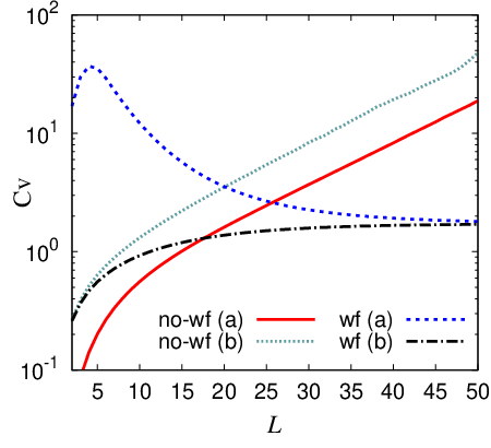
The limitation on the number of independent steps is relatively easy to overcome. The exponential growth of is usually weak, and in most cases, such as the example in Fig. 1, no problems emerge for less than 30 or 50. Moreover, the choice of probabilities that follows importance sampling in Eq. (14) would lead to Practically, numerical noise never allows one to reach this ideal limit but the the growth of variance can be delayed. In addition to that, with a good initial wave function, such as the one from BCS theory, the convergence is reached in a few steps, before the onset of statistical problems; see example in Fig. 1.
Preventing walkers from taking long independent walks, by combining them in wave functions after a certain number of steps with Eq. (8), allows one to avoid the problem completely. This is demonstrated in Fig. 1 with curves labeled “wf”. The intermediate summation at a moment when bags are combined, due to the CLT, prevents an exponential increase of the variance. In the implementation of the CSMC the statistical error is tracked by controlling the coefficient of variation in the bags as is increased. This allows one to apply a computationally expensive procedure of reconstructing the wave function only when necessary, typically once in every 5–20 steps. At a moment when the full wave function is built, the convergence of the projection technique (the second kind of error) can be assessed using the usual square, norm.
The second kind of errors, which is convergence in these examples, is a part of any iterative diagonalization technique, such as Lanczos or Davidson algorithms; and it has been well studied in the past. However, the specifics of the pairing problem described in Sec. II.3 and the use of the linear norm allow one to place exact upper and lower limits on the value of energy.
The convergence of the projection algorithm is examined in Fig. 3. Here, using the same half-occupied ladder model with we show deviation of the predicted energy from the exact value as a function of the number of steps. Three curves, that are essentially indistinct, show where was evaluated using the linear norm Eq. (19). The three sets of results are obtained by evaluating exactly with matrix-vector multiplication (dotted line); using CSMC with wave function being reconstructed at each step (dashed line); and without the wave function using bag average in Eq. (18) (solid line). The slight difference between exact and CSMC results is only due to an intermediate shift by chemical potential. These three curves approach the exact energy from below, which is a distinct property of the norm.
The other two, nearly indistinct, curves show the convergence of energy evaluated using the traditional square norm, labeled as
| (27) |
The norm can be used only when the wave function is available, for that reason only the curves for exact (dash-dot) and CSMC with wave function (short dash) appear in Fig. 3. Naturally, the expectation value of the Hamiltonian in Eq. (27) is subject to the variational principle, and all curves with norm approach ground state energy from above. Thus, the estimates using Eq. (19), and , Eq. (27) norms give the lower and upper bounds for the value of ground state energy.

To summarize, in our algorithm we rely on computationally inexpensive independent propagation of walkers in configuration space until the coefficient of variation of their bags exceeds some critical value. At that moment the full wave function is reconstructed and is used to evaluate energy from Eq. (27) and all other operators of interest. The combination of energy estimates from linear and square norms give lower and upper bounds for the actual value of energy. If the desired convergence is not reached, the process is continued starting from the current wave function.
III.3 Weak pairing limit
As mentioned earlier, superconducting paired states in small systems face a lot of competition from other incoherent interactions as well as from the single particle shell structure. Thus, relatively weak and fragile superconducting states is one of the distinct characteristics of pairing in nuclei. Unfortunately, the BCS theory is not designed to work in this limit, and having the CSMC as a computationally inexpensive alternative is one of the main motivations of this work. In Fig. 4 we demonstrate the effectiveness of CSMC in the limit of weak pairing using our half-filled 18-level ladder model. In the limit when the pairing strength the system settles in the Fermi state with 9 lowest double-degenerate single-particle states being occupied. As soon as pair excitation promotes particles up, and the occupation of the upper 9 levels becomes non-zero. For very strong pairing, the limit of degenerate model with equal occupancy of all states is reached. This limit leads to half of the 18 particles being on lower 9 levels and half on the upper ones.
In Fig. 4 the net occupation of the upper 9 levels as a function of G is shown. This plot includes results from BCS, CSMC (labeled as “MC”) and exact diagonalization. While on a large scale all results are similar, in the region of low pairing strength, which is shown in inset, the well known problem with BCS solution, shown in dotted (black) line, is noticeable. At the same time, exact and CSMC results are indistinct; dashed (crimson color) line goes right on top of the solid (sea-green color) line.

This test illustrates that the CSMC is well suited for all limits of pairing strength. Moreover, in the limit of weak pairing, the computational effort in CSMC is reduced as the contribution from rare excursions above Fermi surface can be easily evaluated with importance sampling.
III.4 Excited states
Obtaining excited states with CSMC is more computationally difficult. One can no longer use a linear norm since all amplitudes cannot be positive definite simultaneously; that is, statement (vi) in Sec.II.3 is not valid for excited states. Therefore, the usual quadratic norm has to be used and the bag values can be negative. Nevertheless, features (i)-(v) in Sec.II.3 remain valid and useful. In particular, since the matrix elements of are positive definite, the importance sampling is still an effective strategy and the signs of bags are not altered by repeated application of the Hamiltonian which curtails the typical MC sign problem. Similar, to Lanczos technique, the CSMC approach requires orthogonalization, therefore the wave functions have to be built each time the orthogonalization is to be performed. The need for orthogonalization limits the number of independent steps, which is the main reason for higher computational demand.
In Fig. 5 we show the CSMC applied to the study of excited states in the same half-occupied 18-level ladder model. The ladder model example is particularly challenging since the density of states above the gap is high. In this model the level spacing between the ground and first excited state, which is about twice the BCS gap, is (in units of level spacing ). At the same time, the spacing between the following states is very small. Moreover, the second excited state is double-degenerate.

III.5 Pairing in Sn isotopes
In order to illustrate the CSMC algorithm in a realistic case where pairing matrix elements are not all equal to a constant, we consider isotopes of tin. The role of pairing in 100-132Sn isotopes has been extensively explored in the literature [53, 28, 10, 29]. Apart from questions of scientific interest such as pairing matrix elements and their connection to superconducting state in infinite matter, near constancy of the excitation energy of the lowest states, and unexplained behavior of electric quadruple transition rates, the tin case emerged as a benchmark for computational techniques. In Tab. 1 we present comparison of energies and occupation numbers for 116Sn, 118Sn, and 120Sn. The model space here includes five single-particle levels (with total ), their energies and spins are listed in the first two columns of Tab. 1, the matrix elements are taken from from the G-matrix calculation in Ref. [54], the values can be found in Table 1 of Ref. [10]. The results in Tab. 1 show expected level of agreement. With increased computational effort, mainly using large number of walkers, any desired level of precision can be obtained; our goal here was to use minimal effort and to solve the pairing problem with a precision that exceeds any practical need, which is set to be 5 keV uncertainty for energy and for occupation numbers.
| 116Sn | 118Sn | 120Sn | |||||
|---|---|---|---|---|---|---|---|
| Exact | CSMC | Exact | CSMC | Exact | CSMC | ||
| j | (MeV) | -153.766 | -153.765 | -170.115 | -170.113 | -185.945 | -185.945 |
| 4.99 | 4.99 | 5.13 | 5.13 | 5.25 | 5.25 | ||
| 5.88 | 5.89 | 6.28 | 6.27 | 6.60 | 6.60 | ||
| 0.67 | 0.67 | 0.76 | 0.76 | 0.86 | 0.86 | ||
| 1.18 | 1.17 | 1.63 | 1.63 | 2.08 | 2.09 | ||
| 3.29 | 3.28 | 4.21 | 4.20 | 5.21 | 5.21 |
III.6 Large scale model
As a final illustration of the CSMC algorithm we explore a model of the 24O nucleus intended to reflect the nature of pairing correlations in a system containing both bound states and a continuum of scattering states. Our main goal is to demonstrate the capabilities of our algorithm while addressing the problem of pairing in continuum qualitatively. Quantitative studies require good knowledge of the effective interaction Hamiltonian; construction of this Hamiltonian is outside the scope of this presentation.
For our study we select the Woods-Saxon potential with parameters from Ref. [55] to model the mean field of weakly-bound 24O nucleus. We discretize this potential using a large quantization-box of size 500 fm. This allows us to generate a dense continuum of states. We limit scattering states by about 8 MeV of energy, which leads to of about 100. For the pairing interaction between neutrons we use a density dependent contact interaction from Refs. [56, 57, 58]
| (28) |
Here is the nucleonic density expressed relative to the saturation density. This quantity is assumed to be given by the Woods-Saxon form factor. The density dependence of pairing is controlled by a parameter which is selected as Following Ref. [56, 58], we also introduce a momentum cut-off function, that gradually reduces the pairing matrix elements to zero for scattering states at energies above 5 MeV, the diffuseness parameter of the cut-off function is 0.5 MeV, see also Ref. [59].
For our example we assume an inert 16O core which leaves two bound and valence single-particle states. Therefore, the bound states can accommodate pairs of valence neutrons in 24O. The pairing matrix elements involving these states are known from the phenomenological shell model Hamiltonian in Ref. [60]. Following previous studies, we adopt the value of GeVfm3 for treating pairing interaction involving the continuum of scattered states. This value is also consistent with the pairing strength in phenomenological Hamiltonians [60]. Here we limit our consideration to -wave single-particle continuum. Due to centrifugal barrier the overlap between bound and unbound -wave states is small; this inhibits virtual pair excitations to -wave states in the continuum.
Our goal in this investigation is to estimate the role of continuum. We do this by comparing full calculation with the one where the continuum is ignored. In Fig. 6 the change in the ground state energy is shown as a function of the single-particle energy of the state. We present two different cases. In case (a) the parameters of the pairing Hamiltonian, which includes the single particle energies and pairing matrix elements, are first evaluated with a realistic choice of Woods-Saxon parameterization for 24O and then the which corresponds to state, is varied while all other parameters remain unchanged. In the self-consistent case (b) the depth of the Woods-Saxon potential is varied which moves the state, and each time a new configuration space Hamiltonian matrix is calculated and studied.
Let us summarize this study. First, the correction from pair excitations into continuum appears to be relatively small, here it is of the order of one kilovolt, for all reasonable choices of pairing strength the effect is not expected to exceed a few tens of kilovolts, see Ref. [59]. The smallness of the effect does not seem to contradict observations. So far there has been no significant near-threshold discontinuity observed in nuclear structure that can be attributed to two-body decay or to pair excitations. The decay of 26O is observed to be very slow, see discussion [61], which through dispersion relations indicates weakness of the continuum coupling.
Second, as expected, the effect increases sharply as the bound state approaches the continuum threshold. This is similar to the results known for single particle states, while the exact near threshold behavior is defined by the phase space volume, see Refs. [62, 63].
Third, the difference between the two models highlights the importance of halo phenomenon and its proper treatment. In model (b) the wave function of the single-particle state spatially extends as its energy approaches the threshold. This facilitates pairing in the continuum and the resulting effect is significantly stronger than that in model (a) where the spatial structure of the single particle wave function was not modified.
Finally, we find that this example successfully demonstrates the power of the CSMC method.

IV Summary
In this work we put forward a new Configuration Space Monte Carlo method for solving the many-body pairing problem in finite systems. Unlike previous Monte Carlo techniques that deal with pairing interaction in a way similar to MC methods in physics of spin systems, our approach does not use evolution in imaginary time, does not need Trotter-Suzuki propagator breakup, and does not depend on the pairing matrix elements being constant. We propose to evaluate Hamiltonian and other observables by stochastically evaluating the corresponding operators in the Krylov subspace spanned by states formed as a result of powers of Hamiltonian acting on an arbitrary initial state. States in the Krylov subspace are evaluated using random walks in the many-body configuration space. Importance sampling is used to effectively probe components of the wave functions. We emphasize several important features of the pairing Hamiltonian, that make the MC approach appealing. In particular, we stress boson-like behavior of nucleon pairs, absence of the fermion sign problem, potential for probabilistic interpretation of transitions in configuration space, and probabilistic interpretation of ground state amplitudes. In addition to traditional quadratic quantum mechanical norm, probabilistic interpretation allows us to use a linear norm. We demonstrate that the approach based on the linear norm is computationally efficient, is perfect for parallelization, and provides effective methods for control of errors of both stochastic and non-stochastic origins.
The workings of the CSMC method are demonstrated with several examples. With a classic ladder model we demonstrate convergence using several variations of the method; we discuss errors and present effective means of their control. The effectiveness of CSMC in small systems where pairing can be effectively weak is shown; the CSMC in its most complete form is used for obtaining degenerate and nearly-degenerate excited states in the ladder model.
As a realistic example, we use isotopes of tin which represents another well studied classic case of pairing in nuclei. The energies and occupation numbers in this non-constant pairing example are consistent with exact results. Large-scale study of pairing correlations is illustrated using a model of 24O that includes a continuum of scattering states. While our last example is still far from realistic, it highlights the effectiveness of CSMC, and suggests an arena for future applications of the method.
Acknowledgements.
This material is based upon work supported by the U.S. Department of Energy Office of Science, Office of Nuclear Physics under Award Number DE-SC0009883.References
- [1] R. A. Broglia and V. Zelevinsky, Fifty years of nuclear BCS (World Scientific, 2013).
- [2] A. Spyrou, Z. Kohley, T. Baumann, D. Bazin, B. A. Brown, G. Christian, P. A. DeYoung, J. E. Finck, N. Frank, E. Lunderberg, et al., Phys. Rev. Lett. 109, 239202 (2012).
- [3] C. R. Hoffman, T. Baumann, J. Brown, P. A. DeYoung, J. E. Finck, N. Frank, J. D. Hinnefeld, S. Mosby, W. A. Peters, W. F. Rogers, et al., Phys. Rev. C 83, 031303 (2011).
- [4] Z. Kohley, E. Lunderberg, P. A. DeYoung, A. Volya, T. Baumann, D. Bazin, G. Christian, N. L. Cooper, N. Frank, A. Gade, et al., Phys. Rev. C 87, 011304 (2013).
- [5] J. Bardeen, L. Cooper, and J. Schrieffer, Phys. Rev. 108, 1175 (1957).
- [6] A. Bohr, B. Mottelson, and D. Pines, Phys. Rev. 110, 936 (1958).
- [7] S. T. Belyaev, K. Dan. Vidensk. Selsk. Mat. Fys. Medd. 11, 31 (1959).
- [8] A. K. Kerman, Ann.Phys. 12, 300 (1961).
- [9] J. Dukelsky, G. G. Dussel, J. G. Hirsch, and P. Schuck, Nucl. Phys. A 714, 63 (2003).
- [10] V. Zelevinsky and A. Volya, Physics of Atomic Nuclei 66, 1829 (2003).
- [11] V. Zelevinsky and A. Volya, Nucl. Phys. A 731, 299 (2004).
- [12] S. C. Pang and A. Klein, Can. J. Phys. 50, 655 (1972).
- [13] J. Y. Zeng and T. S. Cheng, Nucl. Phys. A 405, 1 (1983).
- [14] G. D. Dang and A. Klein, Phys. Rev. 143, 735 (1966a).
- [15] G. D. Dang and A. Klein, Phys. Rev. 147, 689 (1966b).
- [16] H. J. Lipkin, Ann. Phys. 9, 272 (1960).
- [17] Y. Nogami, Phys. Rev. B 134, B313 (1964).
- [18] F. Pan, J. P. Draayer, and W. E. Ormand, Phys. Lett. B 422, 1 (1998).
- [19] A. Volya and V. Zelevinsky, in 13th International Conference on Nuclear Reaction Mechanisms, edited by C. Francesco, M. Chadwick, A. Ferrari, T. Kawano, S. Bottoni, and L. Pellegri (CERN Conference Proceedings Series, Geneva, 2012).
- [20] G. Racah, Phys. Rev. 61, 186 (1942a).
- [21] G. Racah, Phys. Rev. 62, 438 (1942b).
- [22] G. Racah, Phys. Rev. 63, 0367 (1943).
- [23] K. T. Hecht, Phys. Rev. 139, B794 (1965).
- [24] J. N. Ginocchio, Nucl. Phys. 74, 321 (1965).
- [25] N. Auerbach, Nucl. Phys. 76, 321 (1966).
- [26] V. K. B. Kota and J. A. C. Alcaras, Nucl. Phys. A 764, 181 (2006).
- [27] J. Dukelsky and G. Ortiz, Int. J. Mod. Phys. E 15, 324 (2006a).
- [28] B. A. Brown, R. R. C. Clement, H. Schatz, A. Volya, and W. A. Richter, Phys. Rev. C 65, 045802 (2002).
- [29] W.-C. Chen, J. Piekarewicz, and A. Volya, Phys. Rev. C 89, 014321 (2014).
- [30] R. W. Richardson, Phys. Rev. 154, 1007 (1967a).
- [31] R. Richardson, Phys. Rev. 144, 874 (1966).
- [32] R. W. Richardson, Phys. Rev. 159, 792 (1967b).
- [33] R. W. Richardson and N. Sherman, Nucl. Phys. 52, 221 (1964).
- [34] R. W. Richardson, J. Math. Phys. 6, 1034 (1965).
- [35] L. Cooper, Phys. Rev. 104, 1189 (1956).
- [36] J. Dukelsky, S. Pittel, and G. Sierra, Rev. Mod. Phys. 76, 643 (2004).
- [37] S. Pittel and J. Dukelsky, Phys. Scripta T125, 91 (2006).
- [38] J. Dukelsky and G. Ortiz, Int. J. Mod. Phys. E 15, 324 (2006b).
- [39] J. Dukelsky, C. Esebbag, and S. Pittel, Phys. Rev. Lett. 88, 062501 (2002).
- [40] R. R. Whitehead, Nucl. Phys. A 182, 290 (1972).
- [41] A. Volya, B. A. Brown, and V. Zelevinsky, Phys. Lett. B 509, 37 (2001).
- [42] T. Sumaryada and A. Volya, Phys. Rev. C 76, 024319 (2007).
- [43] D. P. Landau and K. Binder, A guide to Monte Carlo simulations in statistical physics (Cambridge University Press, Cambridge, 2005), 2nd ed.
- [44] S. E. Koonin, D. J. Dean, and K. Langanke, Ann. Rev. Nucl. Part. Sc. 47, 463 (1997a).
- [45] S. E. Koonin, D. J. Dean, and K. Langanke, Phys. Rep. 278, 2 (1997b).
- [46] S. C. Pieper and R. B. Wiringa, Ann. Rev. Nucl. Part. Sc. 51, 53 (2001).
- [47] N. Cerf and O. Martin, Phys. Rev. C 47, 2610 (1993).
- [48] N. Cerf, Nucl. Phys. A 564, 383 (1993).
- [49] H. F. Trotter, Proc. Amer. Math. Soc. 10, 545 (1959).
- [50] M. Suzuki, Phys. Lett. A 146 (1990).
- [51] A. Mukherjee, Y. Alhassid, and G. F. Bertsch, Phys. Rev. C 83 014319 (2011).
- [52] Y. Alhassid, A. Mukherjee, H. Nakada, and C. Ozen, J. Phys.: Conf. 403 (2012).
- [53] D. J. Dean and M. Hjorth-Jensen, Rev. Mod. Phys. 75, 607 (2003).
- [54] A. Holt, T. Engeland, M. Hjorth-Jensen, and E. Osnes, Nucl. Phys. A 634, 41 (1998).
- [55] N. Schwierz, I. Wiedenhover, and A. Volya, arXiv:0709.3525 (2007).
- [56] P. Bonche, H. Flocard, P. H. Heenen, S. J. Krieger, and M. S. Weiss, Nucl. Phys. A 443, 39 (1985).
- [57] R. R. Chasman, Phys. Rev. C 14, 1935 (1976).
- [58] J. Dobaczewski, W. Nazarewicz, T. R. Werner, et al., Phys. Rev. C 53, 2809 (1996).
- [59] M. Lingle, Ph.D. thesis, Florida State University (2015).
- [60] B. A. Brown and W. A. Richter, Phys. Rev. C 74, 034315 (2006).
- [61] A. Volya and V. Zelevinsky, Phys. At. Nucl. 77, 969 (2014a).
- [62] A. Volya, EPJ Web of Conf. 38, 03003 (2012).
- [63] A. Volya and V. Zelevinsky, AIP Conf. Proc. 1619, 181 (2014b).